Article

An Autoencoder-like Non-Negative Matrix Factorization with Structure Regularization Algorithm for Clustering

1
School of Statistics and Data Science, Lanzhou University of Finance and Economics, Lanzhou 730020, China
2
Key Laboratory of Digital Economy and Social Computing Science of Gansu, Lanzhou 730020, China
*
Author to whom correspondence should be addressed.
Symmetry 2025, 17(8), 1283; https://doi.org/10.3390/sym17081283
Submission received: 8 July 2025 / Revised: 30 July 2025 / Accepted: 4 August 2025 / Published: 10 August 2025
(This article belongs to the Section Computer)

Abstract

Clustering plays a crucial role in data mining and knowledge discovery, where non-negative matrix factorization (NMF) has attracted widespread attention due to its effective data representation and dimensionality reduction capabilities. However, standard NMF has inherent limitations when processing sampled data embedded in low-dimensional manifold structures within high-dimensional ambient spaces, failing to effectively capture the complex structural information hidden in feature manifolds and sampling manifolds, and neglecting the learning of global structures. To address these issues, a novel structure regularization autoencoder-like non-negative matrix factorization for clustering (SRANMF) is proposed. Firstly, based on the non-negative symmetric encoder-decoder framework, we construct an autoencoder-like NMF model to enhance the characterization ability of latent information in data. Then, by fully considering high-order neighborhood relationships in the data, an optimal graph regularization strategy is introduced to preserve multi-order topological information structures. Additionally, principal component analysis (PCA) is employed to measure global data structures by maximizing the variance of projected data. Comparative experiments on 11 benchmark datasets demonstrate that SRANMF exhibits excellent clustering performance. Specifically, on the large-scale complex datasets MNIST and COIL100, the clustering evaluation metrics improved by an average of 35.31% and 46.17% (ACC) and 47.12% and 18.10% (NMI), respectively.

1. Introduction

Clustering, as an unsupervised learning technique [1], plays a significant role in information retrieval [2], text analysis [3], image clustering [4], and other fields. Common clustering methods include spectral clustering [5], subspace clustering [6], and k-means [7]. However, with the increasing diversity, complexity, and dimensionality of data, redundant information inevitably emerges, posing challenges for clustering analysis. Performing dimensionality reduction on high-dimensional data beforehand—eliminating redundant information while preserving key features—can significantly improve clustering accuracy [8,9,10]. Consequently, following the “reduce-then-cluster” approach, methods such as linear discriminant analysis (LDA) [11], principal component analysis (PCA) [12,13,14], and singular value decomposition (SVD) [15] can be employed for dimensionality reduction. However, these methods may produce negative values in practice, resulting in low-rank matrices with poor interpretability and limited physical meaning after dimensionality reduction.
Non-negative matrix factorization (NMF) [16] adopts a “part-to-whole representation” mechanism, decomposing a data matrix into the product of two non-negative low-rank matrices. It offers advantages such as simplicity in implementation, concise decomposition form, interpretable factor matrices, and reduced storage requirements. NMF has been widely applied in image recognition [17], community detection [18,19,20], and signal processing [21], among other fields. Subsequently, researchers have proposed various extensions of NMF, such as orthogonal NMF (ONMF) by Ding et al. [22] and robust NMF (RNMF) by Kong et al. [23]. With the development of deep learning, Zhao et al. [24] proposed a deep NMF (RDNNBMF), and Hajiveiseh et al. [25] introduced a deep asymmetric NMF (DASNMF). However, these algorithms tend to focus more on reconstruction optimization of the data matrix. To some extent, NMF primarily functions as a decoder: while its non-negativity constraints help preserve the locality of features, it also restrict the linear combination of basis vectors to a non-negative orthant, making it difficult to naturally exhibit desirable properties in low-dimensional representations, such as orthogonality and disentanglement.
To enhance the quality of low-dimensional data representations, researchers have recently proposed manifold learning algorithms such as locally linear embedding (LLE) [26], Laplacian eigenmaps (LE) [27], and isometric mapping (ISOMAP) [28], which describe topological relationships between data through different mapping approaches. Simultaneously, spectral graph theory reflects structural features of data by analyzing the spectral properties of graphs [29]. Within the standard NMF framework, scholars have integrated manifold learning concepts and spectral graph theory by constructing neighborhood graphs to approximate local geometric relationships and capture structural features among data points. For example, Cai et al. [30] proposed graph-regularized NMF (GNMF), which incorporates neighborhood relationships between samples into NMF. Wan et al. [31] introduced robust exponential graph-regularized NMF (REGNMF), employing an exponential graph regularization term to enhance algorithm robustness. Chen et al. [32] incorporated sparsity and orthogonality constraints, proposing orthogonal-graph-regularized NMF with sparse constraints (OGNMFSC). While most studies focus on sample graph learning, some researchers have explored feature graph learning through dual graph regularization. For instance, Shang et al. [33] considered geometric relationships between samples and features, developing dual-graph-regularized NMF (DNMF). Meng et al. [34] proposed sparse and orthogonal dual-graph-regularized NMF (SODNMF). However, these algorithms rely on predefined graph construction methods. To further improve graph learning quality, Huang et al. [35] proposed NMF with adaptive neighborhoods (NMFAN) for dynamic graph structure learning. Ma et al. [36] introduced self-weighted adaptive graph-regularized NMF (SWAGNMF). Nevertheless, these clustering algorithms exhibit certain limitations: they excessively depend on first-order proximity measures between samples, overlook topological similarities across different neighborhood systems, fail to capture high-order graph structural information, and neglect the characterization of global structural distribution. Consequently, they inadequately explore latent relationships between samples [37,38]. With the recent popularity of graph convolutional neural networks (GCNN) [39], high-order similarity information has gained widespread attention. Moreover, in unsupervised learning scenarios where no label information is available, global structure learning can generate more discriminative low-dimensional representations [40]. Studies [40,41,42,43,44,45,46] demonstrate that combining global and local structure learning can better enhance feature learning capability, thereby effectively identifying intrinsic data distributions and improving clustering accuracy.
To address these challenges, a structure regularization autoencoder-like non-negative matrix factorization for clustering (SRANMF) is proposed. Specifically, the principle of a non-negative symmetric encoder-decoder is incorporated into NMF by adopting a bidirectional NMF framework that balances reconstruction accuracy and feature sparsity during low-dimensional representation, thereby improving matrix decomposition accuracy. Simultaneously, to incorporate high-order similarity information, the optimal graph regularization is designed to fully exploit neighborhood structural information, and principal component analysis is employed to learn the global structure of data. This establishes a joint optimization framework synergizing both local and global structure learning. The main contributions of this work are summarized as follows:
(1) A novel NMF clustering algorithm based on structural similarity and autoencoder-like architecture is proposed, which unifies NMF, non-negative symmetric encoder-decoder, optimal graph Laplacian operator, and global structure preservation into a single coherent framework. Due to the symmetry constraints between the decoder and encoder components, the novel approach implicitly imposes quasi-orthogonal constraints on the basis matrix to some extent, avoiding potential redundancy among basis vectors while ensuring necessary independence between feature dimensions.
(2) A local and global structure regularization strategy is developed. It can fully extract high-order neighborhood relationships between samples, effectively capture potential topological correlations among samples, and enhance the representation capability of local manifold structures. Additionally, by utilizing principal component analysis to measure global data structure through maximizing the variance of projected data, this method accurately characterizes the principal structural features of data distribution.
(3) Extensive experiments are conducted on 11 public datasets, demonstrating that SRANMF outperforms 11 state-of-the-art clustering algorithms in terms of clustering accuracy and robustness, validating its superior performance.
The remainder of this paper is organized as follows. Section 2 briefly introduces NMF and graph-regularized non-negative matrix factorization. Section 3 details the proposed algorithm, including its convergence and time complexity analysis. Section 4 presents experimental results and comprehensive analysis. Finally, Section 5 concludes the paper with key findings.

2. Related Work

2.1. Non-Negative Matrix Factorization (NMF)

NMF has attracted wide attention in cluster analysis due to its excellent theoretical and practical value. Lee et al. [16] first proposed the concept of non-negative matrix factorization (NMF), which decomposes a high-dimensional non-negative data matrix X + m × n into the product of two non-negative low-rank matrices, called the basis matrix U + m × r and coefficient matrix V + r × n , where X U V and r min m , n . The loss function is defined using the Frobenius norm, which measures reconstruction error by Euclidean distance. The objective function is formulated as:
min X U V F 2 , s . t . U 0 , V 0
where F denotes the Frobenius norm, and U 0 , V 0 mean all elements are non-negative. According to the multiplicative iterative update rule, the update formulas are:
U i j U i j X V T i j U V V T i j , V i j V i j U T X i j U T U V i j
From the perspective of model architecture, standard NMF is essentially a constrained factorization model that primarily functions as a decoder in clustering tasks, with its core optimization goal focusing on minimizing the global error (such as Frobenius norm or KL divergence) between the original data matrix and the reconstructed matrix. The main limitation of NMF as a decoder is that its linear assumption restricts the modeling capability for complex nonlinear data, and the optimization process is prone to falling into local optima. Meanwhile, the non-negativity constraint causes significant changes in the geometric structure of the latent feature space. Specifically, while the non-negativity constraint enhances feature locality and interpretability by concentrating basis vectors along specific directions, such constraints force data representations to prioritize “part-whole” relationships over global structural relationships, thereby further increasing the complexity of the feature space geometry. To address these issues, inspired by the non-negative symmetric encoder-decoder method proposed by Sun et al. [47] in the field of community detection, an autoencoder-like NMF for cluster analysis is constructed based on the modeling principles of autoencoders.

2.2. Graph-Regularized Non-Negative Matrix Factorization (GNMF)

Standard NMF focuses solely on minimizing the global reconstruction error of the data while neglecting the preservation of local structural information in low-dimensional representations. In recent years, numerous variants of NMF have been proposed to address this limitation. Cai et al. [30] introduced graph-regularized non-negative matrix factorization (GNMF), which incorporates a graph regularization term to constrain variations in the local geometric structure of the data. The objective function of GNMF is:
min X U V F 2 + λ Tr V L V T , s . t . U 0 , V 0
where λ is the regularization parameter ( λ 0 ), and L = D W is the graph Laplacian matrix of the data. Here, W represents the similarity matrix between samples. The degree matrix D = diag ( D 11 , D 22 , , D n n ) is a diagonal matrix with elements satisfying D i i = j W i j . Methods for constructing similarity graphs include k -nearest neighbor graphs, Gaussian kernel similarity graphs, fully connected graphs, and ε -neighborhood graphs. The update rules for the basis matrix U and coefficient matrix V in GNMF are derived as:
U i j U i j X V T i j U V V T i j , V i j V i j U T X + λ W V i j U T U V + λ D V i j
Traditional graph regularization methods typically construct the graph structure solely based on first-order neighborhood relationships between data points. Such a neighborhood-based modeling approach struggles to fully capture the complex structural similarities within the data manifold. To address this, this paper proposes a high-order graph regularization framework that collaboratively learns both the neighborhood relationships and the structural information of local neighborhoods, thereby enabling a multi-level characterization of the intrinsic geometric properties of the data. The specific construction method will be elaborated in Section 3.2.

2.3. Principal Component Analysis (PCA)

PCA preserves global structural information by maximizing the variance of the original data [48] through the construction of a covariance matrix, which captures global correlations among data points without relying on label information [12]. The global mean vector of dataset X is defined as:
x = 1 n i = 1 n x i
The covariance matrix Σ is calculated as:
Σ = i = 1 n x i x x i x T = X I n 1 n e n e n T X T = X C X T
Here, I n is the n × n identity matrix, e n is an n -dimensional column vector with all elements equal to 1, and the centering matrix C = I n 1 n e n e n T . PCA seeks a projection matrix P n × k ( k n ) by maximizing the total variance, with the objective function:
max Tr P T Σ P , s . t . P T P = I k
The projection matrix P obtained from Equation (7) maintains global consistency with the input data.
PCA captures the direction of maximum global variance through orthogonal transformation, but its linear assumption and reliance on second-order statistics limit its ability to model local nonlinear structures (e.g., data manifolds). If only the global variance constraint of PCA is introduced into NMF while ignoring local geometric relationships, the model’s ability to capture the intrinsic manifold structure of the data will be weakened, thereby affecting clustering performance.

3. Methodology

This section details the proposed SRANMF method and its optimization algorithm. Based on the principles of autoencoder modeling, the method incorporates higher-order graph regularization and global structure learning to effectively capture both local and global structural information of the data. By achieving superior low-dimensional representations, it enhances the learning and extraction of deep feature information from the original data, thereby improving clustering accuracy and robustness.

3.1. Autoencoder-like Non-Negative Matrix Factorization

In NMF clustering algorithms, the accuracy of the coefficient matrix V , which serves as the cluster indicator matrix, directly affects the final clustering performance. Traditional NMF methods impose constraints on V only through unidirectional matrix factorization, making it difficult for V to fully capture the underlying structural information of the data. To address this, we adopt a non-negative symmetric encoder-decoder based matrix factorization approach, which enhances the optimization of V by constructing a bidirectional constraint mechanism, thereby improving the stability and representational capability of the coefficient matrix solution.
The data matrix X + m × n is factorized into a basis matrix U + m × r and an encoding matrix V + r × n , i.e., X U V , where this process serves as the decoder, with m being the number of features and n the number of samples. The row vectors of the learned basis matrix U contain feature information of the samples. The decoder aims to find the basis matrix U and encoding matrix V that best reconstruct the original data X , minimizing the loss function:
min X U V F 2 , s . t . U 0 , V 0
The encoder is designed to transform the original spatial structure of the data into a low-dimensional representation. It converts the original matrix X into a distributed representation via the basis matrix U , satisfying V U T X , with the objective function:
min V U T X F 2 , s . t . U 0 , V 0
To ensure that the learned basis matrix U reflects the feature information of the samples, a symmetry constraint is applied to both the decoder and encoder, requiring Equations (8) and (9) to share the same basis matrix U and satisfy the latent constraint U U T = I , which imposes a soft orthogonality constraint on U . Essentially, Equations (8) and (9) seek to maximize the equivalence:
X U V
V U T X
Thus:
X U U T X
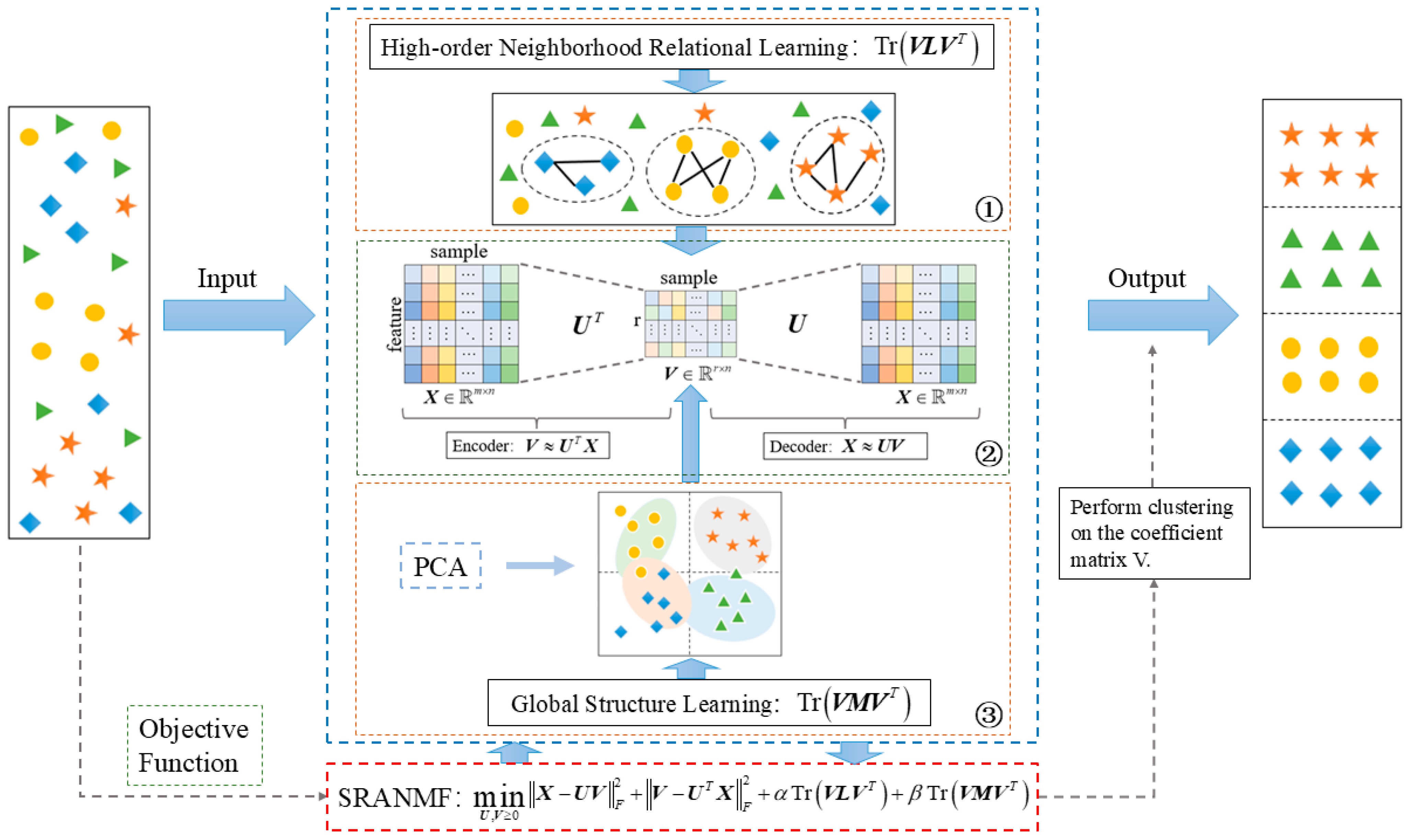
By jointly optimizing the decoder (Equation (8)) and encoder (Equation (9)), an autoencoder-like non-negative matrix factorization framework is proposed, as illustrated in Figure 1. The combined objective function is:
min X U V F 2 d e c o d e r + V U T X F 2 e n c o d e r , s . t . U 0 , V 0
Here, the decoder accounts for data reconstruction error, while the encoder ensures that the product of the transposed basis matrix U T and the original matrix X approximates the low-dimensional representation matrix V . The decoder and encoder share the basis matrix U , subject to symmetry constraints, with an additional soft orthogonality condition U U T = I , ensuring linear independence among the row vectors of U .
Bidirectional non-negative matrix factorization follows the principle of non-negative symmetric encoder-decoder, where data representation is learned through a non-negative symmetric encoder-decoder framework, effectively constituting a specialized form of autoencoder. Based on the multiplicative update rule, the iterative update formulas for Equation (13) are:
V i j V i j 2 U T X i j U T U V + V i j   , U i j U i j 2 X V T i j U V V T + X X T U i j
From Equation (13), it can be observed that although the autoencoder-like NMF minimizes the data reconstruction error through its symmetric encoder-decoder framework, its low-dimensional representation fails to adequately capture the geometric structural features of the data. To address this, we will introduce a higher-order graph regularization method in Section 3.2 and design a global regularization strategy in Section 3.3, aiming to further enhance the quality of low-dimensional representation through the collaborative optimization of global and local structures.

3.2. High-Order Graph Regularization

To better preserve the geometric structure of samples in low-dimensional representations, a graph regularization term is introduced to capture local geometric structures through neighborhood graph learning. To eliminate the influence of heat kernel parameters on graph construction, this paper adopts a binary weighting scheme (0–1 weighting) to define the first-order similarity matrix W 1 in the neighborhood graph.
W 1 i j = 1 , x i N k x j o r x j N k x i 0 , o t h e r w i s e
Here, x i and x j represent the i -th and j -th column samples of the data matrix X , respectively, and N k x j denotes the set of k -nearest data points of sample x j .
Under the assumption of local manifold structure invariance, if x i and x j are neighbors in the original data space, their corresponding vectors v i and v j in the low-dimensional space (matrix V ) should also maintain proximity. Using Euclidean distance to measure inter-sample similarity, the smoothness of the low-dimensional representation is given by:
H 1 = 1 2 i , j = 1 n v i v j 2 W 1 i j = i = 1 n v i v i T D 1 i i i , j = 1 n v i v j T W 1 i j = Tr V D 1 V T Tr V W 1 V T = Tr V L 1 V T
where L 1 = D 1 W 1 is the first-order Laplacian matrix, and D 1 is a diagonal matrix whose elements are the row sums of the similarity matrix W 1 .
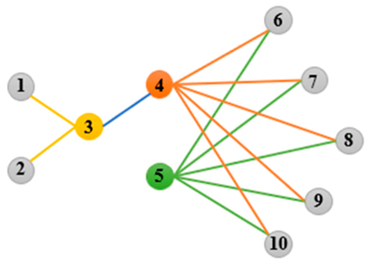
However, in real life, complex relationships between data are widely present. For example, in the process of customer segmentation, even if there is no direct connection between two consumers, when they are associated with a large number of the same user groups, this similarity based on high-order topological structures often accurately clusters them into the same category. Figure 2 illustrates an example of inter-sample associations. As shown in Figure 2, Sample 3 and Sample 4 should exhibit close proximity in the low-dimensional subspace due to their strong direct connection. Similarly, Sample 4 and Sample 5 should also be proximate as they share identical neighbors. In graph embedding encoding, first-order connections reflect proximity relationships between samples but fail to fully uncover their latent relationships. In contrast, second-order connections capture the similarity of neighborhood network structures between samples [37]. Therefore, to better identify potential associations among samples, a polynomial kernel function approach [49,50] is employed to capture higher-order nonlinear relationships between samples. The second-order similarity matrix W 2 is defined as:
W 2 i j = w i T w j
Here, w i and w j are the i -th and j -th column vectors of the first-order similarity matrix W 1 , and L 2 = D 2 W 2 represents the second-order Laplacian matrix. By combining the first-order and second-order Laplacian matrices, the optimal Laplacian matrix is defined as:
L = μ 1 L 1 + μ 2 L 2
where μ 1 and μ 2 are balancing parameters. The optimal graph regularization term is then expressed as:
min V 0 Tr V L V T

3.3. Global Structure Learning

In dimensionality reduction, manifold learning is typically employed to characterize subspace structures for preserving local geometric properties of data. However, in unsupervised learning scenarios where no label information is available, exclusive reliance on local structure learning may lead to the neglect of global structural information in the data space [40]. To address this limitation, principal component analysis (PCA) is utilized to capture global structural relationships among data points, thereby optimizing the coefficient matrix and enhancing the representational capacity of the original data in the low-dimensional space. The global mean vector of the coefficient matrix V = v 1 , v 2 , , v n is:
v = 1 n i = 1 n v i
The representation of global structure learning is expressed as:
max i = 1 n v i v 2 2 = i = 1 n v i T v i 2 v i T v + v T v = i = 1 n v i T v i 1 n i = 1 n v i T v = Tr V V T 1 n Tr V e n e n T V T = Tr V I n 1 n e n e n T V T = Tr V C V T
Equation (21) represents a regularization term derived from variance maximization of the input data that seeks to maximize the objective during optimization. However, this conflict with the NMF framework, which adopts a minimization strategy. Therefore, to unify the optimization direction, let M = C = 1 n e n e n T I n = E n I n , where E n = 1 n e n e n T ; then:
min V 0 Tr V M V T

3.4. Objective Function

By integrating Equations (13), (19) and (22), the objective function of SRANMF is formulated as:
min U , V 0 X U V F 2 + V U T X F 2 + α Tr V L V T + β Tr V M V T
where both α and β are non-negative regularization parameters. The first term ( X U V F 2 ) functions as a decoder, aiming to decompose high-dimensional data into two low-dimensional matrices by controlling the reconstruction error. The second term ( V U T X F 2 ) serves as an encoder, designed to further explore latent relationships among data through distributed representations of the original data matrix. The third term ( Tr V L V T ) learns the local structure by capturing high-order neighborhood relationships of samples, thereby improving the quality of their low-dimensional representations. The fourth term ( Tr V M V T ) learns the global distribution characteristics of the data by maximizing the variance direction. The combination of the first and second terms forms an autoencoder-like bidirectional NMF framework, optimizing data fidelity, thereby enhancing the representational capacity of SRANMF for raw data. The integration of the third and fourth terms enables SRANMF to preserve both local and global structural features of the data under the synergistic effects of regularization parameters α and β , thereby improving clustering accuracy and generalization capability. Figure 3 presents the schematic diagram of the proposed SRANMF.

3.5. Optimization Algorithm

SRANMF employs multiplicative update rules for iterative optimization. The augmented Lagrangian function of the objective function in Equation (23) is formulated as:
J U , V = X U V F 2 + V U T X F 2 + α Tr V L V T + β Tr V M V T Tr Λ 1 U T Tr Λ 2 V T
Here, Λ 1 + m × r and Λ 2 + r × n are the Lagrange multipliers for U and V , respectively, which present as penalty terms to enforce non-negativity constraints for U and V .
Equation (24) can be expanded and have terms independent of U and V eliminated.
L U , V = Tr V T U T U V 2 V T U T X + Tr V T V 2 V T U T X + X T U U T X + α Tr V L V T + β Tr V M V T Tr Λ 1 U T Tr Λ 2 V T
Then, L U , V takes partial derivatives with respect to U and V , respectively, yielding:
L U = 2 U V V T 4 X V T + 2 X X T U Λ 1
L V = 2 U T U V 4 U T X + 2 V + 2 α V L + 2 β V M Λ 2
Since V has non-negativity constraints while the Laplacian matrix L contains negative off-diagonal elements, L in Equation (27) can be factorized as L = L + L , where L + = ( | L | + L ) / 2 and L = ( | L | L ) / 2 .
Equation (27) can then be rewritten as:
L V = 2 U T U V 4 U T X + 2 V + 2 α V L + 2 α V L + 2 β V E n 2 β V I n Λ 2
According to the KKT conditions ( Λ 1 ) i j U i j = 0 and ( Λ 2 ) i j V i j = 0 :
( 2 U V V T 4 X V T + 2 X X T U Λ 1 ) i j   U i j = 0
( 2 U T U V 4 U T X + 2 V + 2 α V L + 2 α V L + 2 β V E n 2 β V I n Λ 2 ) i j V i j = 0
This further obtains:
( 2 U V V T 4 X V T + 2 X X T U Λ 1 ) i j   U i j 2 = 0
( 2 U T U V 4 U T X + 2 V + 2 α V L + 2 α V L + 2 β V E n 2 β V I n Λ 2 ) i j V i j 2 = 0
Consequently, the update rules for U and V are:
U i j t + 1 U i j t 2 X V T i j U V V T + X X T U i j
V i j t + 1   V i j t 2 U T X + α V L + β V I n i j U T U V + V + α V L + + β V E n i j

3.6. Convergence Analysis

In this section, the convergence of the SRANMF algorithm is proven using the auxiliary function approach.
First, the convergence with respect to V is proven. For clarity, terms involving only the matrix V are retained in the objective function, while others unrelated to V are discarded. This results in a new function F i j V i j :
F i j V i j = Tr V T U T U V 2 V T U T X + Tr V T V 2 V T U T X + α Tr V L + V T α Tr V L + V T + β Tr V E n V T β Tr V I n V T = Tr ( V T U T U V 4 V T U T X + V T V + α V L + V T α V L V T + β V E n V T β V I n V T )
An auxiliary function G V i j , V i j t for F i j V i j is defined as:
G V i j , V i j t = i j U T U V t i j V i j 2 V i j t 4 i j U T X i j V i j t 1 + log V i j V i j t + i j V i j 2 + α i j V t L + i j V i j 2 V i j t α i j l L j l V i j t V i l t 1 + log V j l V i l V j l t V i l t + β i j V t E n i j V i j 2 V i j t β i j l I n j l V i j t V i l t 1 + log V j l V i l V j l t V i l t
Next, it is demonstrated that the constructed function G V i j , V i j t serves as an auxiliary function for F i j V i j .
Proof. 
When V i j = V i j t , it satisfies G V i j , V i j = F i j V i j . To prove G V i j , V i j t F i j V i j , consider the following:
For symmetric matrices A and B , the following inequality (37) holds:
i = 1 n j = 1 m A S t B i j S i j 2 S i j t Tr S T A S B , A + n × n , B + m × m , S t + n × m , S + n × m
Thus, it can be derived:
Tr V T U T U V   i j ( U T U V t ) i j V i j 2 V i j t
Tr V T V i j V i j 2
α Tr V L + V T α i j V t L + i j V i j 2 V i j t
β Tr V E n V T β i j V t E n i j V i j 2 V i j t
Using the inequality x > 1 + log x x > 0 , the following can be obtained:
4 Tr V T U T X = 4 Tr X T U V 4 i j U T X i j V i j t 1 + log V i j V i j t
α Tr V L V T α i j l   L j l V i j t V i l t 1 + log V j l V i l V j l t V i l t
β Tr V I n V T β i j l I n j l V i j t V i l t 1 + log V j l V i l V j l t V i l t
From Equations (38)–(44), it follows that G V i j , V i j t F i j V i j . Therefore, G V i j , V i j t is an auxiliary function for F i j V i j .
By setting G V , V t V i j = 0 , the following can be obtained:
V i j t + 1   V i j t 2 U T X + α V L + β V I n i j U T U V + V + α V L + + β V E n i j
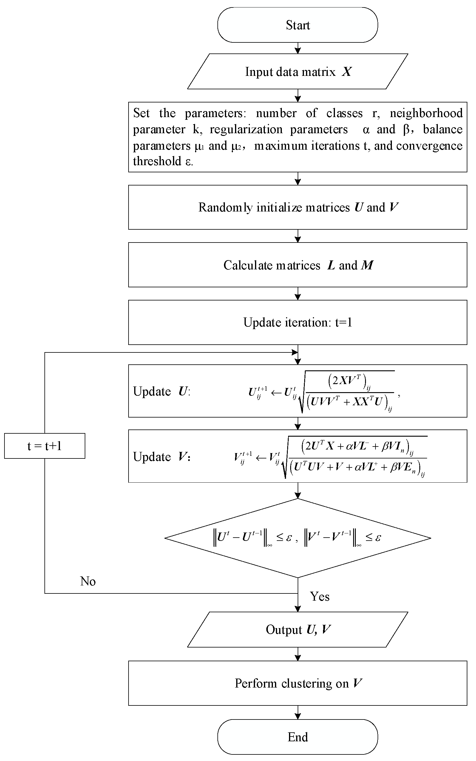
Hence, under the update rule (34), the matrix V in the SRANMF algorithm is guaranteed to be non-increasing, thereby ensuring convergence. Similarly, it can be shown that U is also non-increasing under the update rule (33), with convergence guaranteed. In conclusion, the SRANMF algorithm is proven to converge under the update rules (33) and (34). The detailed implementation of SRANMF is outlined in Algorithm 1. Figure 4 shows the flowchart of Algorithm 1. □
Algorithm 1. Structure Regularization Autoencoder-Like Non-Negative Matrix Factorization for Clustering (SRANMF)
Input: Initial matrix X = x 1 , x 2 , , x n + m × n , number of categories r , neighborhood parameter k , regularization parameters α and β , balance parameters μ 1 and μ 2 , maximum number of iterations t , threshold ε = 1 0 - 4 .
Output: Basis matrix U and coefficient matrix V .
1. Initialization: Randomly generate basis matrix U m × r and coefficient matrix V r × n ;
2. Calculate the optimal Laplacian matrix L according to Equations (15)–(18);
3. Calculate matrix M according to Equations (20)–(22);
4. Update basis matrix U according to Equation (33);
5. Update coefficient matrix V according to Equation (34);
6. Termination: When U t U t 1 ε and V t V t 1 ε .
7. Finally, obtain the clustering indicator matrix V , and apply k-means to cluster the coefficient matrix V .

3.7. Time Complexity Analysis

In Algorithm 1, the time complexity of SRANMF mainly consists of steps 2–5. For data matrix X m × n , where m represents the number of features and n represents the number of samples. Assuming the number of categories is r ( r min m , n ), after the t -th iteration, the computational cost for updating basis matrix U and coefficient matrix V are O t m 2 r + t m r 2 and O t m 2 r + t m r 2 + m n 2 . Therefore, the time complexity of the proposed SRANMF algorithm is derived as O t m 2 r + m n 2 . Here, the time complexity of SRANMF is compared with that of the algorithms used in the experiments in Section 4. The specific comparison is shown in Table 1.
As shown in Table 1, the SRANMF algorithm exhibits certain complexity characteristics in terms of time complexity. In Section 4, comprehensive experiments will be conducted to further validate the clustering performance of the SRANMF.

4. Experiments and Analysis

In this section, experiments are conducted on 11 datasets to evaluate the performance of the proposed SRANMF algorithm. Comparative analysis is performed between SRANMF and 11 representative algorithms in terms of clustering performance. The experiments are implemented in Python 3.11, and the computer environment for the experiments is an Intel(R) Core (TM) i5-1135G7 @ 2.40 GHz 2.42 GHz processor with 16 GB memory and a Windows 11 64-bit operating system.

4.1. Dataset

The Cacmcisi and MM datasets are sourced from the CLUTO toolkit (https://conservancy.umn.edu/items/4fbef165-f964-41ed-a239-86a8f931ffbe, accessed on 15 December 2024); The Semeion and Wdbc datasets are obtained from the UCI Machine Learning Repository (https://archive.ics.uci.edu, accessed on 15 December 2024); The COIL20 (http://www.cs.columbia.edu/CAVE/software/softlib/coil-20.php, accessed on 15 December 2024) and COIL100 (http://www.kaggle.com/jessicali9530/coil100/downloads/coil100.zip/2, accessed on 15 December 2024) datasets consist of images capturing 20 and 100 objects recorded at different rotational angles, respectively; The MINIST2k2k, Mnist05, and MNIST datasets (http://yann.lecun.com/exdb/mnist/, accessed on 15 December 2024) are collections of handwritten digits; The FERET32x32 dataset (https://www.nist.gov/itl/products-and-services/color-feret-database, accessed on 15 December 2024) contains facial images of 200 individuals under varying illumination conditions; The UMIST dataset (https://opendatalab.org.cn/OpenDataLab/UMIST, accessed on 15 December 2024) comprises face images of 20 different individuals. The basic information of the 11 datasets is shown in Table 2.

4.2. Dataset Clustering Performance Evaluation Metrics

To obtain more objective results, this paper evaluates the clustering performance of each algorithm on the dataset using four common clustering evaluation metrics.

4.2.1. Clustering Accuracy (ACC)

ACC = i = 1 n δ m a p s i , r i n
In Equation (46), n represents the number of samples, s i denotes the label obtained from the clustering algorithm for the i -th instance, and r i represents the true label of the data. Here, δ m a p s i , r i is defined as:
δ m a p s i , r i = 1 , m a p s i = r i 0 , m a p s i r i

4.2.2. Adjusted Rand Index (ARI)

ARI = i j n i j 2 i x i 2 j y i 2 / n 2 0.5 i x i 2 + j y i 2 i x i 2 j y i 2 / n 2
In Equation (48), n is the total number of samples; n i j represents the number of samples that are simultaneously in the i -th cluster of the algorithm and the j -th true class; x i denotes the number of samples in the i -th cluster obtained by the algorithm; and y j represents the number of samples in the j -th true class.

4.2.3. Normalized Mutual Information (NMI)

NMI N , N * = MI N , N * max H N , H N *
In Equation (49), N represents the true labels, and N * denotes the labels obtained from the clustering algorithm. Here, H is the entropy function, and MI represents the mutual information (MI), whose mathematical expression is:
MI N , N * = n i N , n j * N * p n i , n j * log p n i , n j * p n i p n j *
In Equation (50), p n i is the probability that a sample belongs to the true class n i , p ( n j * ) is the probability that a sample belongs to the clustered class n j * , and p n i , n j * is the joint probability that a sample simultaneously belongs to the true class n i and the clustered class n j * .

4.2.4. Clustering Purity (PUR)

PUR = i = 1 r max j n i j n
In Equation (51), n i j represents the number of samples in the i -th cluster that belong to the true class j .
The four clustering evaluation metrics introduced above yield higher values when the clustering performance of the algorithm is better. Among them, ARI has a range of 1 , 1 , while the other three metrics have a range of [ 0 , 1 ] .

4.3. Comparative Algorithms and Parameter Settings

This experiment compared a total of 11 clustering algorithms, as detailed below:
(1) NMF [16]: NMF decomposes a high-dimensional non-negative matrix into two low-rank non-negative matrices, and then optimizes these two submatrices by building up a global reconstruction error function.
(2) RNMF [23]: Based on standard NMF, the l 2 , 1 -norm is adopted to measure reconstruction errors, thereby enhancing robustness against noise and outliers.
(3) NMFOS [51]: To mitigate redundant information interference in NMF, NMFOS introduces orthogonal constraints into the objective function to improve data independence and algorithm performance.
(4) GNMF [30]: GNMF incorporates the geometric structure information among samples into the objective function based on NMF, thereby improving the quality of the low-dimensional representation.
(5) LCCF [52]: Building on concept factorization (CF) [55], LCCF adds graph regularization to improve clustering performance.
(6) RSGNMF [53]: RSGNMF employs the l 2 , 1 -norm for robustness, imposes sparsity penalties on features, and integrates local structure learning to further enhance performance.
(7) RSNMF [40]: RSNMF jointly optimizes non-negative matrix factorization and the basis matrix using the l 2 , 1 -norm, with added global and local structural constraints.
(8) RSCNMF [46]: This algorithm combines global and local structure optimization during matrix decomposition to improve clustering.
(9) REGNMF [31]: Extending GNMF, REGNMF introduces exponential graph regularization (exponentiating the Laplacian matrix) to boost robustness and clustering performance.
(10) LS-NMF [54]: LS-NMF applies logarithmic norm constraints on factor matrices for sparsity.
(11) OGNMFSCUU [32]: A multi-objective optimization model is developed by incorporating orthogonality, sparsity, and other constraints during matrix decomposition to refine clustering performance.
Table 1 lists the objective functions of the above algorithms. Among them, RSNMF and RSCNMF consider the local-global information, while SRANMF not only considers the local-global information, but also further mines the data information by introducing a non-negative symmetric encoder-decoder architecture.
For all the above algorithms, the regularization parameters are optimized using a grid search method within the ranges specified in Table 3 (for specific parameter definitions, please refer to Table 1).
Table 4 shows the values of the high-order graph regularization parameter α and the global structure regularization parameter β for SRANMF across different datasets.

4.4. Results and Analysis

During the experiments, clustering results are observed to exhibit stochastic fluctuations. To mitigate this variability and ensure stable clustering outcomes, each algorithm is executed 20 times on each of the 11 datasets, and the average values and standard deviations are calculated as the final clustering results. Table 5, Table 6, Table 7 and Table 8 present the detailed numerical results of the four clustering evaluation metrics for the 12 algorithms across the 11 datasets. Boldfaced values in the tables indicate the best clustering performance for that particular dataset run.
As evidenced by Table 5, Table 6, Table 7 and Table 8, it can be observed that SRANMF achieves the highest values across all four clustering evaluation metrics on these 11 datasets, demonstrating its excellent clustering performance and robustness.
(1) Compared to clustering algorithms without structural constraints (NMF, RNMF, NMFOS), SRANMF significantly improves clustering performance. Specifically, SRANMF shows average improvements of 21.21%, 26.68%, and 20.99% over NMF, RNMF, and NMFOS, respectively, in ACC values; SRANMF shows average improvements of 47.35%, 67.00%, and 47.51% over NMF, RNMF, and NMFOS, respectively, in ARI values; SRANMF shows average improvements of 28.43%, 36.71%, and 28.32% over NMF, RNMF, and NMFOS, respectively, in NMI values; and SRANMF shows average improvements of 21.39%, 23.80%, and 21.05% over NMF, RNMF, and NMFOS, respectively, in PUR values. These results clearly indicate SRANMF outperforms structure-unconstrained clustering algorithms in clustering performance.
(2) When compared to locally constrained clustering algorithms (GNMF, LCCF, RSGNMF, REGNMF, LS-NMF, OGNMFSCUU), SRANMF demonstrates superior clustering performance. For instance, on the COIL100 dataset, the optimal metric values of SRANMF are observed to exceed those of the six algorithms by 10.98% (ACC), 14.92% (ARI), 7.49% (NMI), and 17.06% (PUR). On the UMIST dataset, the improvements are 39.65% (ACC), 48.18% (ARI), 18.28% (NMI), and 31.54% (PUR). SRANMF consistently achieves higher evaluation metric values than these six algorithms across all datasets.
(3) Compared to globally and locally constrained clustering algorithms (RSNMF, RSCNMF), SRANMF not only improves clustering performance but also enhances robustness. Comprehensive analysis of the four evaluation metrics shows that SRANMF achieves average performance improvements of 28.18% over RSNMF and 40.52% over RSCNMF. Specifically, SRANMF improves ACC by 21.43% over RSNMF and 32.00% over RSCNMF; ARI by 49.36% over RSNMF and 71.80% over RSCNMF; NMI by 29.24% over RSNMF and 40.97% over RSCNMF; and PUR by 21.58% over RSNMF and 31.37% over RSCNMF. Additionally, SRANMF generally exhibits lower standard deviations than RSNMF or RSCNMF, indicating reduced variability and enhanced stability of its clustering outcomes.
These experimental results demonstrate the excellent clustering performance of SRANMF. Compared to RSNMF and RSCNMF (which jointly model local and global structural features), the advantage of SRANMF lies in its adoption of a bidirectional NMF framework inspired by autoencoder principles, which thoroughly exploit latent data representations. Moreover, during local structure learning, SRANMF captures high-order neighborhood relationships among samples by constructing both first-order and second-order Laplacian matrices.
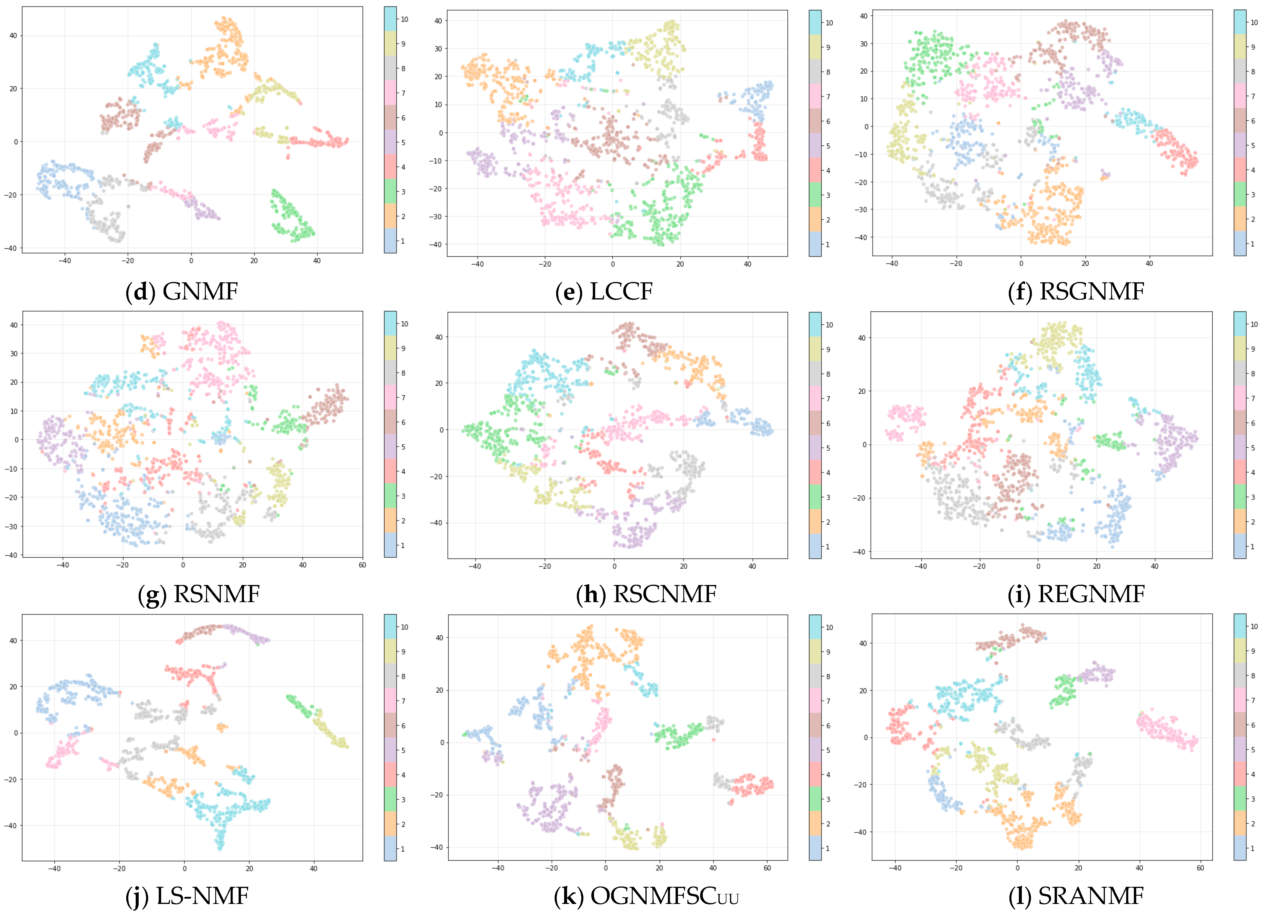
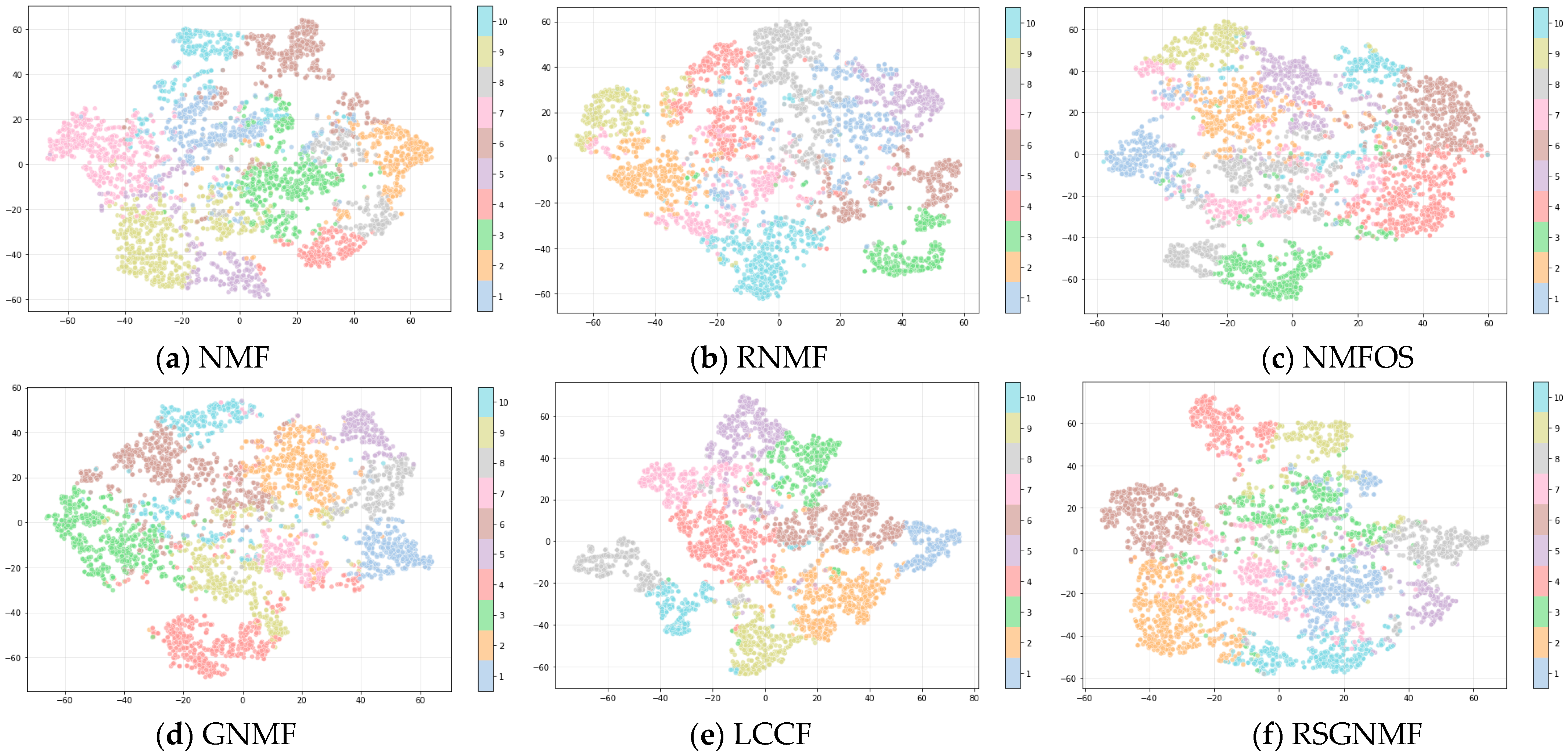
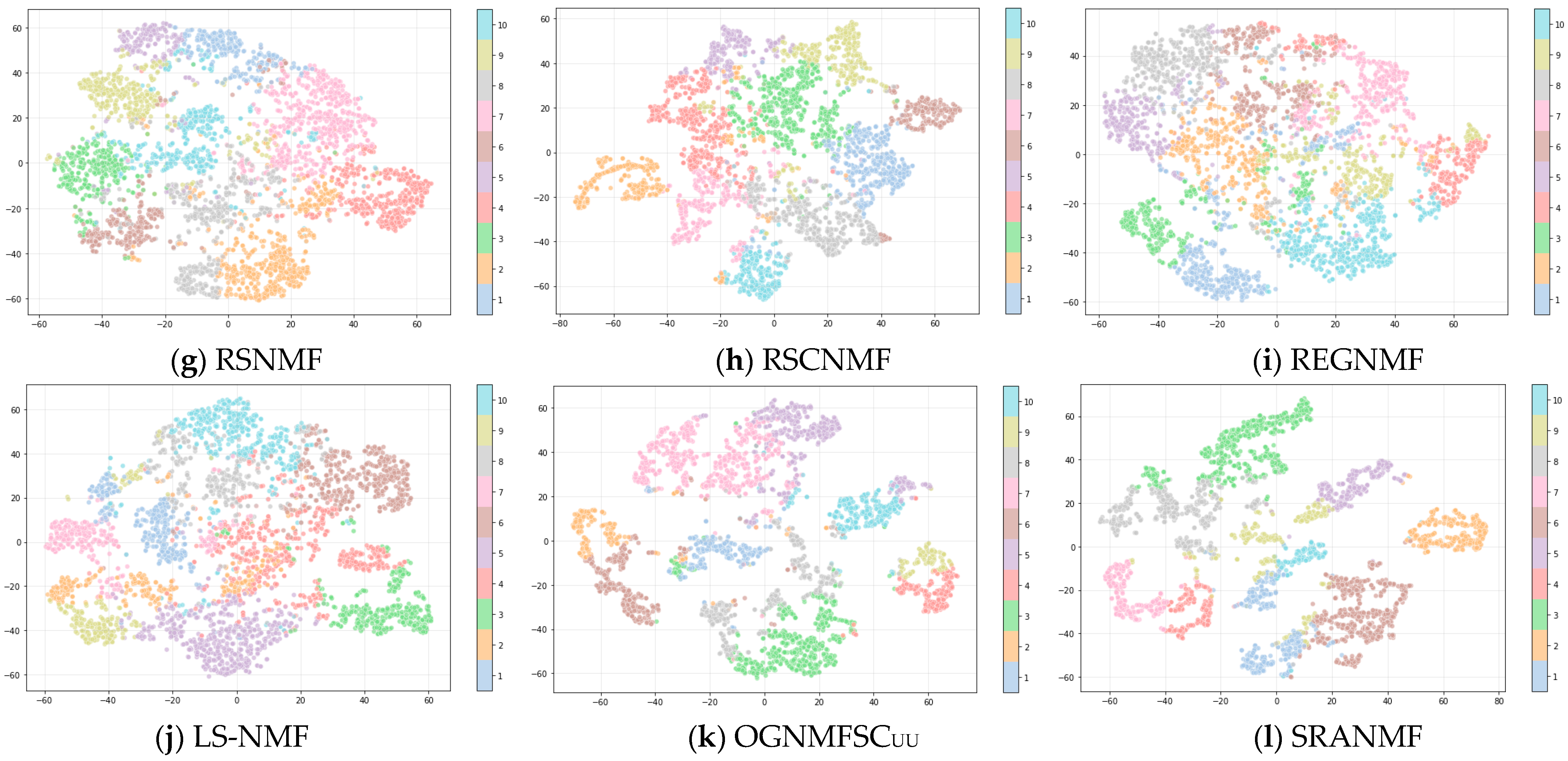
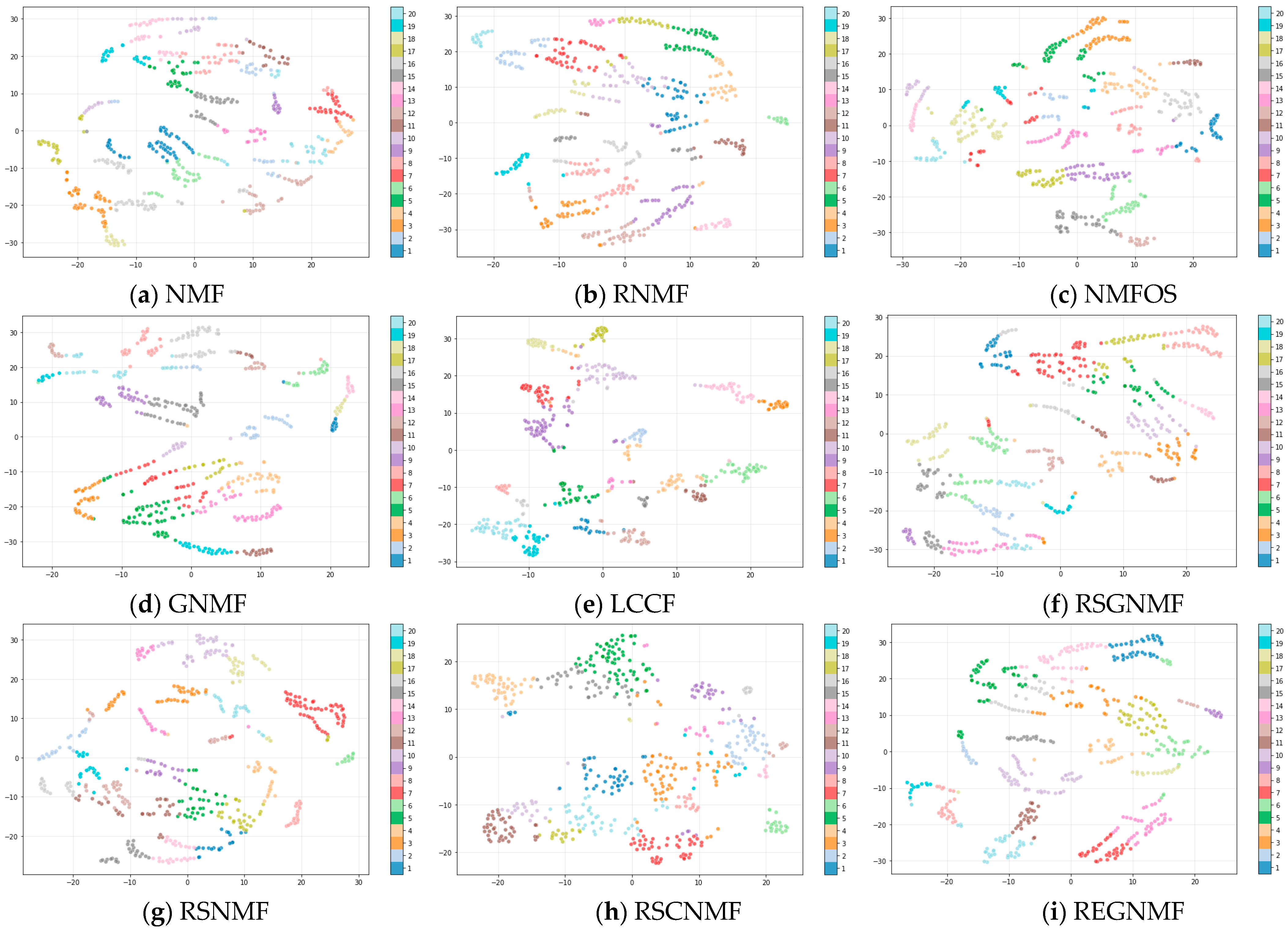
To further visually demonstrate the clustering performance of the SRANMF algorithm, the t-SNE method is employed to project the low-dimensional data obtained by the 12 algorithms into a two-dimensional space and generate visualization plots. Due to space limitations, three datasets with a relatively large number of categories—Semeion, MINIST2k2k, and UMIST—are selected as representatives. The comparative visualization plots of the proposed SRANMF algorithm and the other 11 clustering algorithms on these three datasets are presented in Figure 5, Figure 6 and Figure 7, respectively.
As can be seen from Figure 5, Figure 6 and Figure 7, the low-rank submatrix obtained through dimensionality reduction of high-dimensional data matrices via the SRANMF algorithm demonstrates more significant intra-class compactness and inter-class separation. Therefore, when dealing with high-dimensional data clustering problems, the SRANMF algorithm can first be employed for dimensionality reduction, followed by applying the k-means method to cluster the obtained low-rank submatrix, which will significantly improve the accuracy of clustering results.

4.5. Ablation Experiments

SRANMF consists of three components: data reconstruction error measurement based on autoencoder-like NMF, high-order graph regularization term, and global structure learning term. To rigorously evaluate the contributions of global and local structural information extraction from the data space on clustering performance, a “0” value is assigned to the regularization parameters α and β , thereby controlling each term. When both parameters α and β are 0, SRANMF degenerates into SRANMF-1, which contains only the data fitting term. Here, SRANMF-1 is mathematically equivalent to NSED [47] in terms of the objective function. Comparative analysis between SRANMF and SRANMF-1 validates the synergistic effect of integrating high-order graph regularization learning with global structure learning. When α = 0 and β > 0 , SRANMF degenerates into SRANMF-2, which includes only the data fitting term and the regularization term for global structure learning. Systematic variation of β quantifies the impact of the regularization term for global structure learning on clustering performance. When α > 0 and β = 0 , SRANMF degenerates into SRANMF-3, which includes only the data fitting term and the high-order graph regularization term. Parametric adjustment of α isolates the contribution of the high-order graph regularization term to clustering performance. By comparing the clustering performance of SRANMF-1, SRANMF-2, SRANMF-3, and SRANMF, an in-depth discussion is conducted regarding the independent roles of the high-order graph regularization term and the global structure regularization term in the clustering process, emphasizing the necessity and effectiveness of their joint optimization.
Furthermore, to examine the data representation capability of the autoencoder-like bidirectional NMF, the encoder part is removed from SRANMF, resulting in SRANMF-4, which degenerates into a unidirectional NMF. Additionally, since SRANMF fully considers the first-order and second-order similarities between data samples during local structure learning, the impact of second-order neighborhood connections on clustering results is investigated by eliminating the second-order Laplacian matrix term from SRANMF. This process results in SRANMF-5, where L 1 is the first-order Laplacian matrix constructed in Equation (16). Table 9 shows the objective functions corresponding to the degraded versions of SRANMF, while Table 10 and Table 11 present the experimental results comparing clustering performance.
Table 10 and Table 11 show that SRANMF outperforms all its degraded variants across all clustering evaluation metrics (ACC, ARI, NMI, PUR). This empirically demonstrates that the joint optimization of autoencoder-like bidirectional NMF, high-order graph regularization, and global structure regularization not only enhances clustering performance and robustness but also improves generalization capability. Compared to SRANMF-1, SRANMF-2, and SRANMF-3, SRANMF achieves average performance improvements of 23.57%, 24.24%, and 3.22%, respectively. Similarly, SRANMF shows average improvements of 20.86% and 10.33% over SRANMF-4 and SRANMF-5, respectively. Detailed analysis follows:
(1) The clustering performance of SRANMF is significantly superior to SRANMF-1. Since SRANMF incorporates high-order graph regularization and global structure regularization terms beyond SRANMF-1, it achieves average improvements of 18.84% (ACC), 39.61% (ARI), 24.58% (NMI), and 17.64% (PUR) over SRANMF-1.
(2) SRANMF-2 demonstrates suboptimal generalization capability with potential overfitting issues, despite exhibiting competitive performance on specific datasets. For instance, SRANMF-2 performs better than SRANMF-1 only on FERET32x32 (ACC, ARI, NMI, PUR), UMIST (ACC), MM (ACC, ARI, NMI, PUR), and Semeion (ARI, NMI) metrics, while underperforming on other comparisons. Since this study uses maximized projection data variance to measure global data structure, the orthogonal constraints on the potential clustering indicator matrix V may cause the decomposition results to deviate from the true data distribution, thereby reducing clustering performance when only global structure is considered.
(3) Although SRANMF-3 shows significant performance improvements, inherent limitations are observed. By adding high-order graph regularization to SRANMF-1, SRANMF-3 significantly improves clustering performance by capturing local geometric features. However, on the FERET32x32 dataset, SRANMF-2 outperforms SRANMF-3, suggesting that global regularization may outweigh high-order graph regularization for specific datasets. This phenomenon reveals that excessive focus on local features may neglect global structures, weakening generalization.
(4) Comparing SRANMF with SRANMF-4 confirms the superiority of autoencoder-like bidirectional NMF for clustering. SRANMF improves clustering performance over SRANMF-4 by 1.00–45.48% (ACC), 5.35–87.35% (ARI), 3.70–167.54% (NMI), and 1.00–37.32% (PUR).
(5) The necessity of high-order neighborhood modeling is validated by comparing SRANMF with SRANMF-5. On average, SRANMF improves clustering performance by 8.48% (ACC), 17.68% (ARI), 10.22% (NMI), and 7.46% (PUR) compared to SRANMF-5.
SRANMF employs a predefined graph construction strategy during the graph learning process, rather than a dynamic graph learning mechanism, which differs from adaptive graph-regularized NMF. Simultaneously, SRANMF currently focuses solely on modeling the sample graph and does not consider the learning of the feature graph. Inspired by dual-graph-regularized NMF, future research could further explore strategies for simultaneously learning both the sample graph and the feature graph to enhance the algorithm’s performance.

4.6. Parameter Sensitivity Analysis

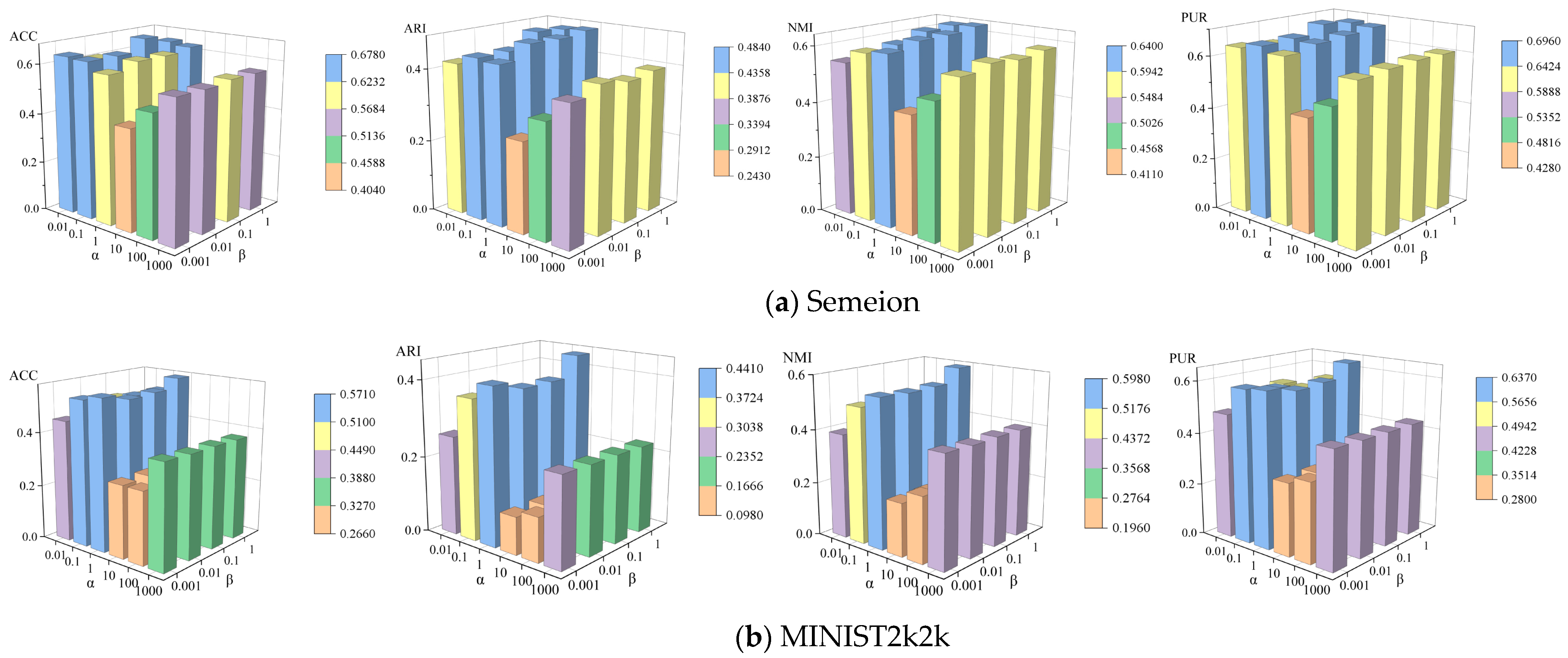
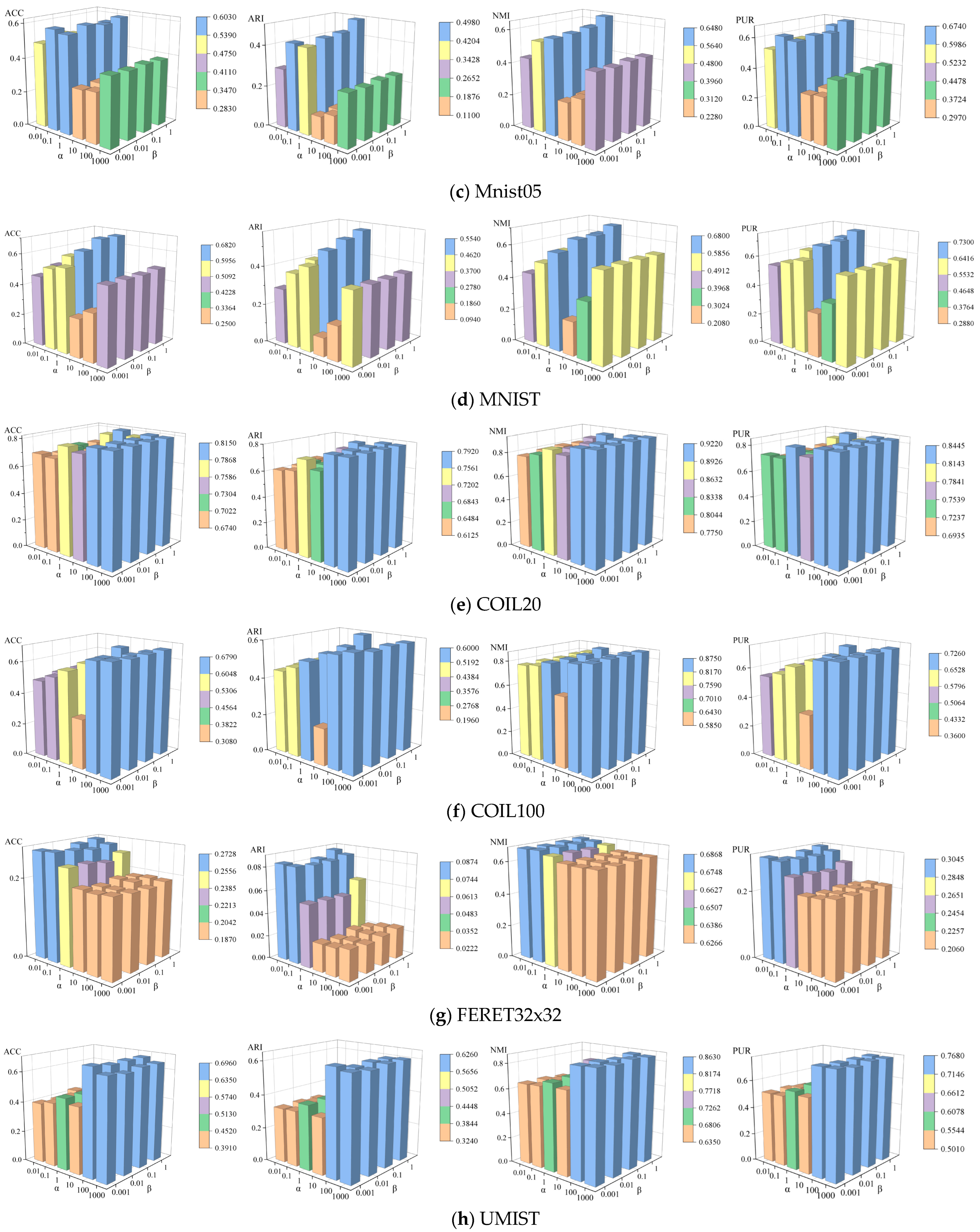
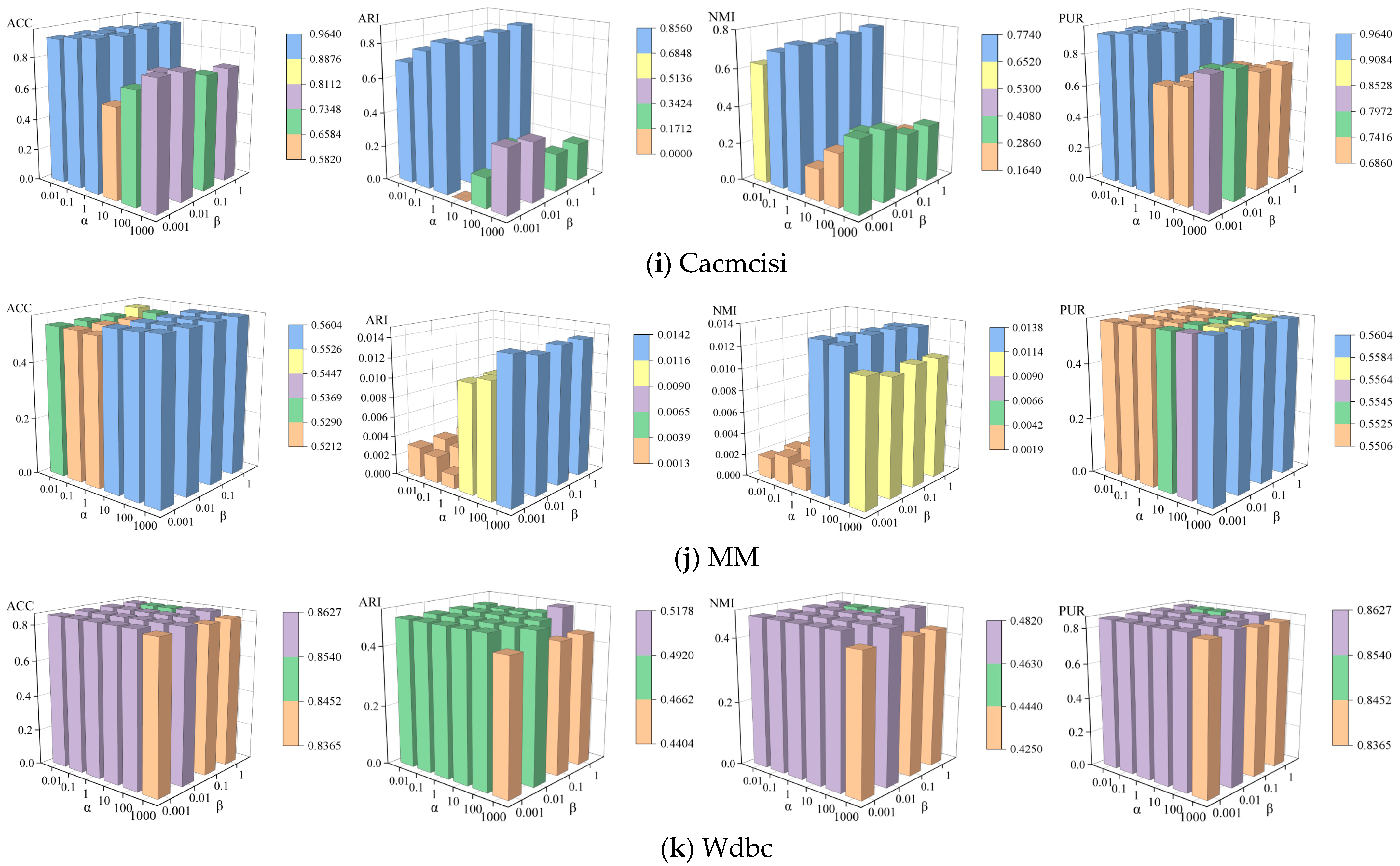
The proposed SRANMF introduces two hyperparameters: the high-order graph regularization coefficient α and the global structure learning regularization coefficient β . To test the algorithm’s sensitivity to these parameters, one parameter is fixed while the other is varied over a wide range. The value ranges for α and β are { 10 2 , 10 1 , 10 0 , 10 1 , 10 2 , 10 3 } and { 10 3 , 10 2 , 10 1 , 10 0 } , respectively. To ensure balanced visualization across different orders of magnitude, logarithmic scaling is applied to the values of α and β during plotting. The parameter sensitivity analysis for α and β is shown in Figure 8.
From Figure 8, the following conclusions can be drawn:
(1) SRANMF exhibits higher sensitivity to the high-order graph regularization parameter α than to the global structure learning regularization parameter β . When α is fixed, changes in β have minimal impact on clustering results. However, when β is fixed, variations in α significantly affect clustering performance.
(2) On the COIL20, COIL100, and UMIST datasets, SRANMF demonstrates superior clustering performance when parameter α is set to larger values. However, on the FERET32x32 dataset, the clustering performance of SRANMF deteriorates with larger α values. Therefore, the optimal selection of parameter α should be adjusted based on the specific feature distribution of each dataset.

4.7. Empirical Convergence

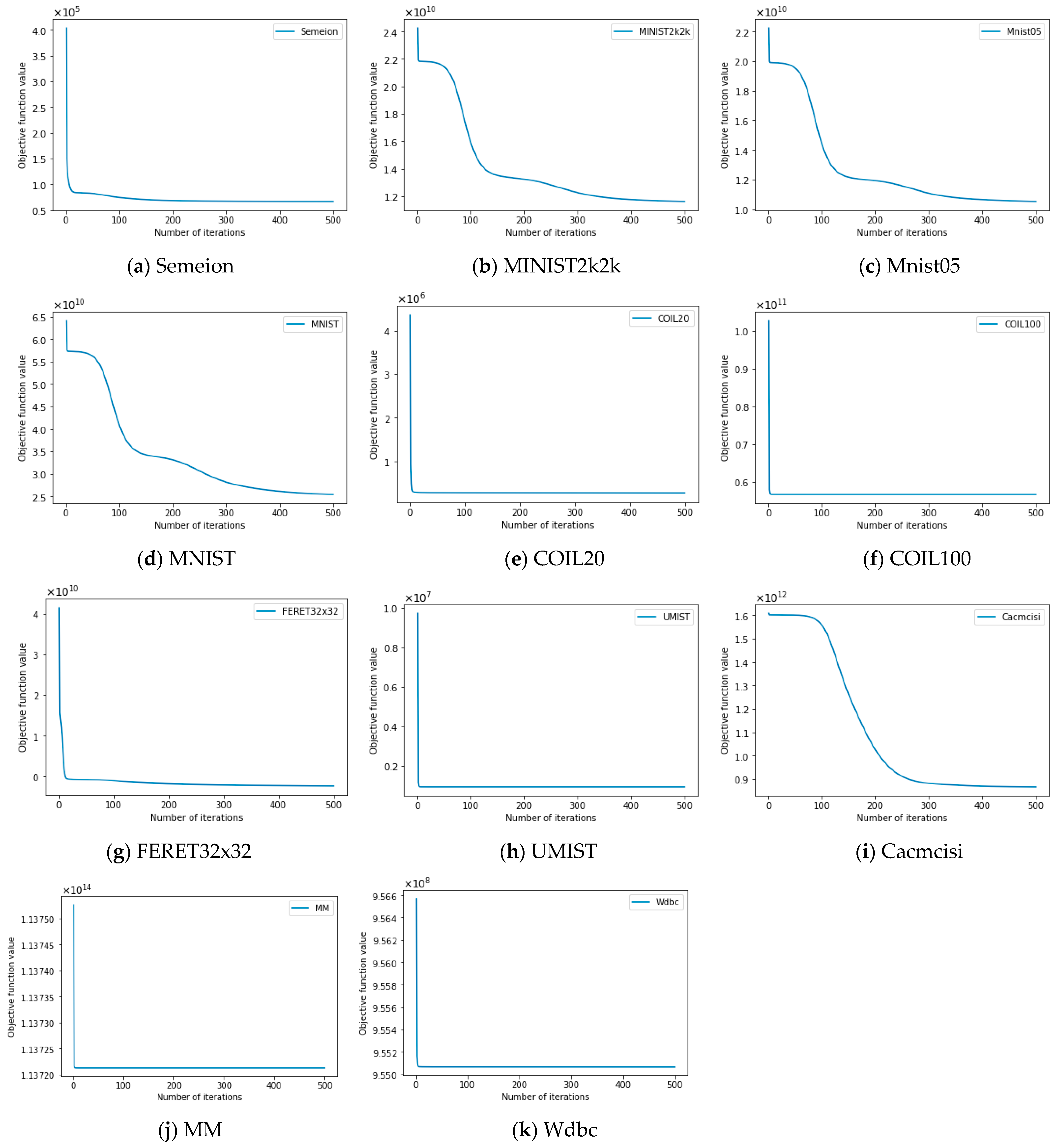
In Section 3.3, the convergence of the algorithm was proven from the perspective of theoretical analysis. In this section, we further validate the convergence of the SRANMF algorithm from an experimental perspective. In the experiments, the values of the hyperparameters α and β in SRANMF still adopt the numerical values listed in Table 4. Figure 9 illustrates the convergence curves of SRANMF on the 11 datasets.
As shown in Figure 9, SRANMF achieves rapid convergence on the COIL20, COIL100, UMIST, MM, and Wdbc datasets. On the Semeion and FERET32x32 datasets, SRANMF achieves stable convergence after approximately 200 iterations. On the Cacmcisi dataset, the convergence speed of the SRANMF algorithm is initially slow; after 100 iterations, the convergence rate accelerates, ultimately achieving convergence around 300 iterations. For the MINIST2k2k, Mnist05, and MNIST datasets, the objective function value of the SRANMF algorithm first rapidly decreases, subsequently enters a plateau phase, resumes a rapid decline, and finally stabilizes around 400 iterations, thereby achieving convergence.

4.8. Runtime Analysis

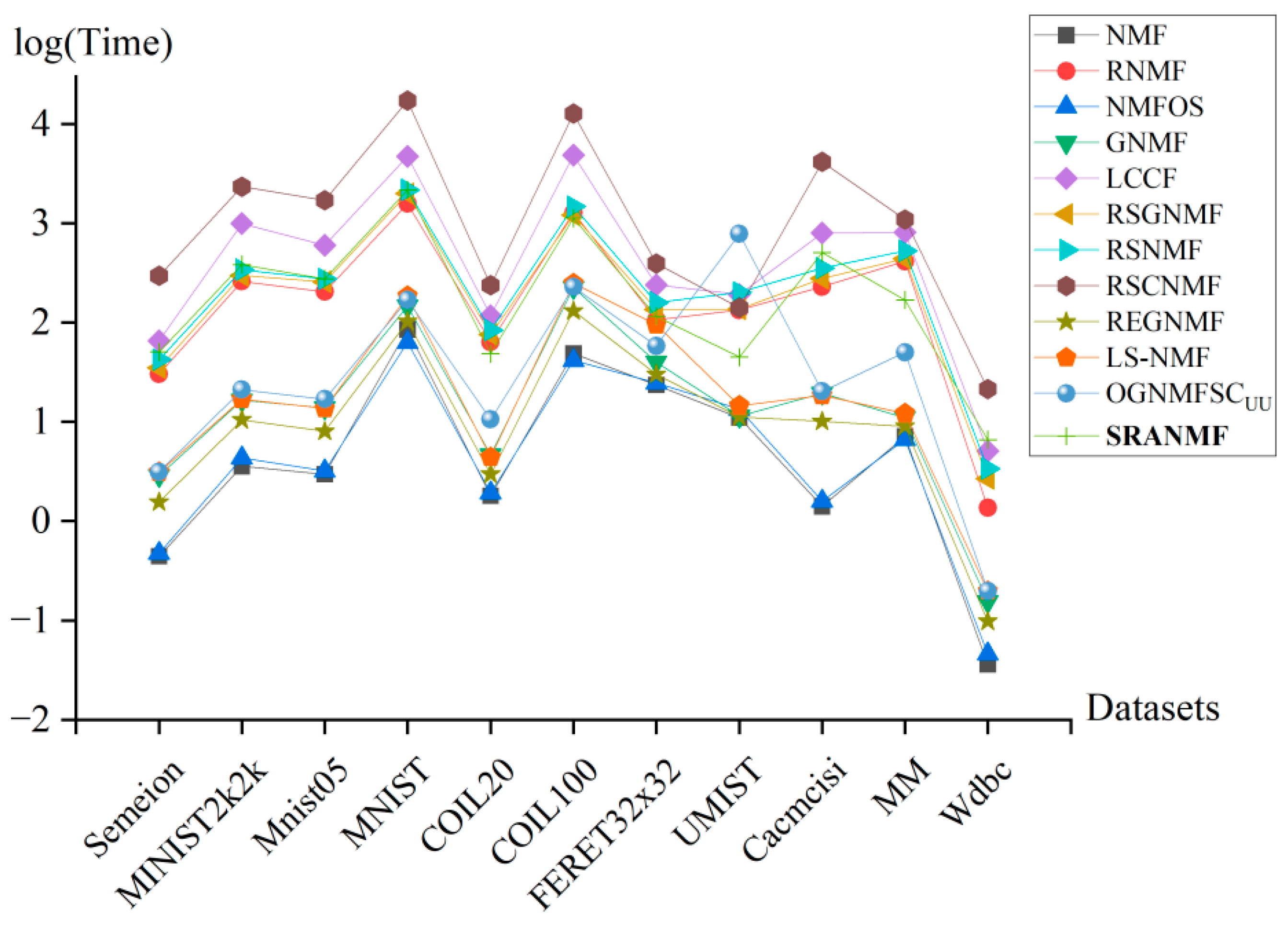
To further analyze the computational speed of each algorithm, a comparative study of the runtime per-iteration for these 12 algorithms across 11 datasets is performed. The runtime comparison is visualized using a logarithmic scale for the time axis, with specific results as shown in Figure 10. The running time of each algorithm is recorded in milliseconds.
From Figure 10, it can be observed that NMF and NMFOS demonstrate faster computational speeds on these 11 datasets, while LCCF and RSCNMF show slower computational speeds. Although SRANMF ranks in the middle-to-lower range among these 12 algorithms in terms of per-iteration runtime, it achieves superior performance in clustering tasks.

5. Conclusions

This paper proposes a structure regularization autoencoder-like non-negative matrix factorization for clustering (SRANMF). The algorithm employs a non-negative symmetric encoder-decoder model to enhance the quality of matrix factorization and introduces an optimal Laplacian matrix to capture high-order neighborhood relationships for local graph structure learning, thereby thoroughly exploring deep feature information within the data. Additionally, by incorporating PCA principles, the true distribution characteristics of internal data structures are extracted to learn global data structures. Finally, comprehensive experiments comparing SRANMF with 11 other advanced clustering algorithms on 11 public datasets demonstrate the superior clustering performance of SRANMF across four clustering metrics. The ablation studies reveal that: (1) the autoencoder-like NMF further optimizes data fitting, thereby enhancing the representational capacity of SRANMF for original data; (2) the integration of first-order and second-order Laplacian matrices enables effective capture of high-order neighborhood relationships and latent topological structures between samples; and (3) high-order graph regularization and global structure regularization exhibit complementarity, jointly improving the clustering performance and generalization capability of SRANMF.
The SRANMF algorithm significantly improves clustering performance, but due to its high computational complexity, its runtime efficiency when handling high-dimensional complex data still needs to be enhanced. The work has certain limitations, and future improvements will be pursued in the following directions. Firstly, the current SRANMF is built solely on a single-layer NMF framework. Subsequent efforts will extend it to deep non-negative matrix factorization (DNMF) architecture, aiming to enhance model representational capacity and learning performance. Secondly, SRANMF is currently limited to unsupervised learning scenarios. A semi-supervised learning variant will be investigated by incorporating limited labeled data to strengthen model generalization and practicality. Finally, adaptive graph regularization techniques will be incorporated to the SRANMF framework to better capture intrinsic data relationships through dynamic adjustment of graph structure weights, thereby further improving model robustness and adaptability.

Author Contributions

Conceptualization, H.G. and L.Z.; methodology, H.G. and L.Z.; software, H.G. and L.Z.; validation, H.G. and L.Z.; formal analysis, H.G. and L.Z.; investigation, H.G. and L.Z.; resources, H.G.; data curation, L.Z.; writing—original draft preparation, H.G. and L.Z.; writing—review and editing, H.G. and L.Z.; visualization, L.Z.; supervision, H.G.; project administration, H.G. and L.Z.; funding acquisition, H.G. All authors have read and agreed to the published version of the manuscript.

Funding

This work was funded by the National Social Science Fund of China (NO. 21BTJ042), the Gansu Provincial Natural Science Foundation (NO. 23JRRA1186), and the Gansu Provincial Universities’ Young Doctor Support Program (NO. 2025QB-058).

Data Availability Statement

Publicly available datasets were analyzed in this study.

Acknowledgments

The authors sincerely appreciate the editors and reviewers for their valuable comments and professional suggestions.

Conflicts of Interest

The authors declare no conflicts of interest.

References

  1. Huang, S.; Ren, Y.; Xu, Z. Robust multi-view data clustering with multi-view capped-norm K-means. Neurocomputing 2018, 311, 197–208. [Google Scholar] [CrossRef]
  2. Xing, Z.; Wen, M.; Peng, J.; Feng, J. Discriminative semi-supervised non-negative matrix factorization for data clustering. Eng. Appl. Artif. Intell. 2021, 103, 104289. [Google Scholar] [CrossRef]
  3. Aghdam, M.H.; Zanjani, M.D. A novel regularized asymmetric non-negative matrix factorization for text clustering. Inf. Process. Manag. 2021, 58, 102694. [Google Scholar] [CrossRef]
  4. Liu, M.; Yang, Z.; Han, W.; Chen, J.; Sun, W. Semi-supervised multi-view binary learning for large-scale image clustering. Appl. Intell. 2022, 52, 14853–14870. [Google Scholar] [CrossRef]
  5. He, W.; Zhang, S.; Li, C.G.; Qi, X.; Xiao, R.; Guo, J. Neural normalized cut: A differential and generalizable approach for spectral clustering. Pattern Recogn. 2025, 164, 111545. [Google Scholar] [CrossRef]
  6. Deng, T.; Ye, D.; Ma, R.; Fujita, H.; Xiong, L. Low-rank local tangent space embedding for subspace clustering. Inf. Sci. 2020, 508, 1–21. [Google Scholar] [CrossRef]
  7. Zhao, X.; Nie, F.; Wang, R.; Li, X. Robust fuzzy k-means clustering with shrunk patterns learning. IEEE Trans. Autom. Control 2023, 35, 3001–3013. [Google Scholar] [CrossRef]
  8. Nie, F.; Huang, H.; Cai, X.; Ding, C.H.Q. Efficient and robust feature selection via joint ℓ2,1-norms minimization. Adv. Neural Inf. Process. Syst. 2010, 23, 1813–1821. Available online: https://proceedings.neurips.cc/paper/2010/file/09c6c3783b4a70054da74f2538ed47c6-Paper.pdf (accessed on 25 May 2025).
  9. Shang, R.; Zhang, Z.; Jiao, L.; Liu, C.; Li, Y. Self-representation based dual-graph regularized feature selection clustering. Neurocomputing 2016, 171, 1242–1253. [Google Scholar] [CrossRef]
  10. Shang, R.; Wang, W.; Stolkin, R.; Jiao, L. Non-negative spectral learning and sparse regression-based dual-graph regularized feature selection. IEEE Trans. Cybern. 2018, 48, 793–806. [Google Scholar] [CrossRef]
  11. Yang, X.; Cao, C.; Zhou, K.; Peng, S.; Wang, Z.; Lin, L.; Nie, F. A novel linear discriminant analysis based on alternate ratio sum minimization. Inf. Sci. 2025, 689, 121444. [Google Scholar] [CrossRef]
  12. Wold, S.; Esbensen, K.; Geladi, P. Principal component analysis. Chemom. Intell. Lab. Syst. 1987, 2, 37–52. [Google Scholar] [CrossRef]
  13. Hu, Z.; Pan, G.; Wang, Y.; Wu, Z. Sparse principal component analysis via rotation and truncation. IEEE Trans. Neural Netw. Learn. Syst. 2016, 27, 875–890. [Google Scholar] [CrossRef]
  14. Yata, K.; Aoshima, M. Effective PCA for high-dimension, low-sample-size data with noise reduction via geometric representations. J. Multivar. Anal. 2011, 105, 193–215. [Google Scholar] [CrossRef]
  15. Zhang, Q.; Wang, Y.; Levine, M.D.; Li, X. Multisensor video fusion based on higher order singular value decomposition. Inf. Fusion 2015, 24, 54–71. [Google Scholar] [CrossRef]
  16. Lee, D.D.; Seung, H.S. Learning the parts of objects by non-negative matrix factorization. Nature 1999, 401, 788–791. [Google Scholar] [CrossRef] [PubMed]
  17. Kriebel, A.R.; Welch, J.D. UINMF performs mosaic integration of single-cell multi-omic datasets using nonnegative matrix factorization. Nat. Commun. 2022, 13, 780. [Google Scholar] [CrossRef] [PubMed]
  18. Lu, H.; Sang, X.; Zhao, Q.; Lu, J. Community detection algorithm based on nonnegative matrix factorization and pairwise constraints. Phys. A Stat. Mech. Appl. 2020, 545, 123491. [Google Scholar] [CrossRef]
  19. Fan, D.; Zhang, X.; Kang, W.; Zhao, H.; Lv, Y. Video watermarking algorithm based on NSCT, pseudo 3D-DCT and NMF. Sensors 2022, 22, 4752. [Google Scholar] [CrossRef] [PubMed]
  20. Zhao, Z.; Ke, Z.; Gou, Z.; Guo, H.; Jiang, K.; Zhang, R. The trade-off between topology and content in community detection: An adaptive encoder-decoder-based NMF approach. Expert Syst. Appl. 2022, 209, 118230. [Google Scholar] [CrossRef]
  21. Kwon, K.; Shin, J.W.; Kim, N.S. NMF-based speech enhancement using bases update. IEEE Signal Process. Lett. 2015, 22, 450–454. [Google Scholar] [CrossRef]
  22. Ding, C.; Li, T.; Peng, W.; Park, H. Orthogonal nonnegative matrix t-factorizations for clustering. In Proceedings of the 12th ACM SIGKDD International Conference on Knowledge Discovery and Data Mining, New York, NY, USA, 20–23 August 2006; pp. 126–135. [Google Scholar] [CrossRef]
  23. Kong, D.; Ding, C.; Huang, H. Robust nonnegative matrix factorization using L21-norm. In Proceedings of the 20th ACM International Conference on Information and Knowledge Management, New York, NY, USA, 24–28 October 2011; pp. 673–682. [Google Scholar] [CrossRef]
  24. Zhao, Y.; Wang, H.; Pei, J. Deep Non-Negative Matrix Factorization Architecture based on Underlying Basis Images Learning. IEEE Trans. Pattern Anal. Mach. Intell. 2021, 43, 1897–1913. [Google Scholar] [CrossRef]
  25. Hajiveiseh, A.; Seyedi, S.A.; Akhlaghian, T.F. Deep asymmetric nonnegative matrix factorization for graph clustering. Pattern Recogn. 2024, 148, 110179. [Google Scholar] [CrossRef]
  26. Roweis, S.T.; Saul, L.K. Nonlinear dimensionality reduction by locally linear embedding. Science 2000, 290, 2323–2326. [Google Scholar] [CrossRef]
  27. Belkin, M.; Niyogi, P. Laplacian eigenmaps and spectral techniques for embedding and clustering. Adv. Neural Inf. Process. Syst. 2001, 14, 585–591. Available online: https://dl.acm.org/doi/10.5555/2980539.2980616 (accessed on 7 July 2025).
  28. Balasubramanian, M.; Schwartz, E.L. The Isomap algorithm and topological stability. Science 2002, 295, 7. [Google Scholar] [CrossRef] [PubMed]
  29. Dhanjal, C.; Gaudel, R.; Clémençon, S. Efficient eigen-updating for spectral graph clustering. Neurocomputing 2014, 131, 440–452. [Google Scholar] [CrossRef]
  30. Cai, D.; He, X.; Han, J.; Huang, T.S. Graph regularized nonnegative matrix factorization for data representation. IEEE Trans. Pattern Anal. Mach. Intell. 2010, 33, 1548–1560. [Google Scholar] [CrossRef]
  31. Wan, M.; Cai, M.; Yang, G. Robust exponential graph regularization non-negative matrix factorization technology for feature extraction. Mathematics 2023, 11, 1716. [Google Scholar] [CrossRef]
  32. Chen, Y.; Qu, G.; Zhao, J. Orthogonal graph regularized non-negative matrix factorization under sparse constraints for clustering. Expert Syst. Appl. 2024, 249, 123797. [Google Scholar] [CrossRef]
  33. Shang, F.; Jiao, L.C.; Wang, F. Graph dual regularization non-negative matrix factorization for co-clustering. Pattern Recogn. 2012, 45, 2237–2250. [Google Scholar] [CrossRef]
  34. Meng, Y.; Shang, R.; Jiao, L.; Zhang, W.; Yang, S. Dual-graph regularized non-negative matrix factorization with sparse and orthogonal constraints. Eng. Appl. Artif. Intell. 2018, 69, 24–35. [Google Scholar] [CrossRef]
  35. Huang, S.; Xu, Z.; Kang, Z.; Ren, Y. Regularized nonnegative matrix factorization with adaptive local structure learning. Neurocomputing 2020, 382, 196–209. [Google Scholar] [CrossRef]
  36. Ma, Z.; Wang, J.; Li, H.; Huang, Y. Adaptive graph regularized non-negative matrix factorization with self-weighted learning for data clustering. Appl. Intell. 2023, 53, 28054–28073. [Google Scholar] [CrossRef]
  37. Tang, J.; Qu, M.; Wang, M.; Zhang, M.; Yan, J.; Mei, Q. LINE: Large-scale information network embedding. In Proceedings of the 24th International Conference on World Wide Web, Florence, Italy, 18–22 May 2015; pp. 1067–1077. [Google Scholar] [CrossRef]
  38. Bu, X.; Wang, G.; Hou, X. Motif-based mix-order nonnegative matrix factorization for community detection. Phys. A Stat. Mech. Appl. 2025, 661, 130350. [Google Scholar] [CrossRef]
  39. Defferrard, M.; Bresson, X.; Vandergheynst, P. Convolutional neural networks on graphs with fast localized spectral filtering. Adv. Neural Inf. Process. Syst. 2016, 29, 3844–3852. [Google Scholar] [CrossRef]
  40. Huang, Q.; Yin, X.; Chen, S.; Wang, Y.; Chen, B. Robust nonnegative matrix factorization with structure regularization. Neurocomputing 2020, 412, 72–90. [Google Scholar] [CrossRef]
  41. Zhang, D.; He, J.; Zhao, Y.; Luo, Z.; Du, M. Global plus local: A complete framework for feature extraction and recognition. Pattern Recogn. 2014, 47, 1433–1442. [Google Scholar] [CrossRef]
  42. de Silva, V.; Tenenbaum, J.B. Global versus local methods in nonlinear dimensionality reduction. Adv. Neural Inf. Process. Syst. 2002, 15, 721–728. Available online: https://dl.acm.org/doi/10.5555/2968618.2968708 (accessed on 7 July 2025).
  43. Zhou, N.; Xu, Y.; Cheng, H.; Fang, J.; Pedrycz, W. Global and local structure preserving sparse subspace learning: An iterative approach to unsupervised feature selection. Pattern Recogn. 2016, 53, 87–101. [Google Scholar] [CrossRef]
  44. Chen, J.; Ye, J.; Li, Q. Integrating global and local structures: A least squares framework for dimensionality reduction. In Proceedings of the 2007 IEEE Conference on Computer Vision and Pattern Recognition, Minneapolis, MN, USA, 17–22 June 2007; pp. 1–8. [Google Scholar] [CrossRef]
  45. Liu, X.; Wang, L.; Zhang, J.; Yin, J.; Liu, H. Global and local structure preservation for feature selection. IEEE Trans. Neural Netw. Learn. Syst. 2014, 25, 1083–1095. [Google Scholar] [CrossRef]
  46. Yang, Q.; Yin, X.; Kou, S.; Wang, Y. Robust structured convex nonnegative matrix factorization for data representation. IEEE Access 2021, 9, 155087–155102. [Google Scholar] [CrossRef]
  47. Sun, B.J.; Shen, H.; Gao, J.; Ouyang, W.; Cheng, X. A Non-negative symmetric encoder-decoder approach for community detection. In Proceedings of the 2017 ACM Conference on Information and Knowledge Management, New York, NY, USA, 6–10 November 2017; pp. 597–606. Available online: https://dl.acm.org/doi/10.1145/3132847.3132902 (accessed on 7 July 2025).
  48. Wang, H.; Nie, F.; Huang, H. Globally and locally consistent unsupervised projection. In Proceedings of the Twenty-Eighth AAAI Conference on Artificial Intelligence, Québec City, QC, Canada, 27–31 July 2014; pp. 1328–1333. Available online: https://dl.acm.org/doi/10.5555/2893873.2894079 (accessed on 7 July 2025).
  49. Vishwanathan, S.V.N.; Schraudolph, N.N.; Kondor, R.; Borgwardt, K.M. Graph kernels. J. Mach. Learn. Res. 2010, 11, 1201–1242. Available online: https://jmlr.csail.mit.edu/papers/volume11/vishwanathan10a/vishwanathan10a.pdf (accessed on 13 May 2025).
  50. Xu, L.; Niu, X.; Xie, J.; Abel, A.; Luo, B. A local-global mixed kernel with reproducing property. Neurocomputing 2015, 168, 190–199. [Google Scholar] [CrossRef]
  51. Li, Z.; Wu, X.; Peng, H. Nonnegative matrix factorization on orthogonal subspace. Pattern Recogn. Lett. 2010, 31, 905–911. [Google Scholar] [CrossRef]
  52. Cai, D.; He, X.; Han, J. Locally consistent concept factorization for document clustering. IEEE Trans. Knowl. Data Eng. 2011, 23, 902–913. [Google Scholar] [CrossRef]
  53. Yang, S.; Hou, C.; Zhang, C.; Wu, Y.; Weng, S. Robust non-negative matrix factorization via joint sparse and graph regularization. In Proceedings of the 2013 International Joint Conference on Neural Networks (IJCNN), Dallas, TX, USA, 4–9 August 2013; pp. 1–5. [Google Scholar] [CrossRef]
  54. Peng, C.; Zhang, Y.; Chen, Y.; Kang, Z.; Chen, C.; Cheng, Q. Log-based sparse nonnegative matrix factorization for data representation. Knowl.-Based Syst. 2022, 251, 109127. [Google Scholar] [CrossRef]
  55. Xu, W.; Gong, Y. Document clustering by concept factorization. In Proceedings of the 27th Annual International ACM SIGIR Conference on Research and Development in Information Retrieval, New York, NY, USA, 25–29 July 2004; pp. 202–209. [Google Scholar] [CrossRef]
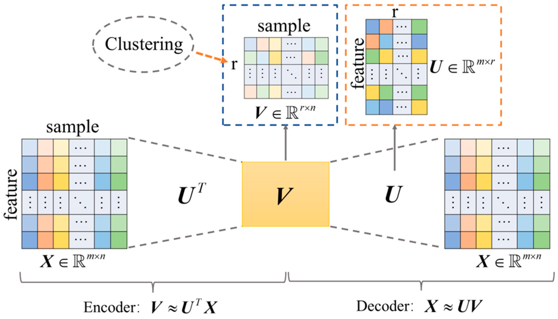
Figure 1. Schematic diagram of the non-negative symmetric encoder-decoder-based matrix factorization.
Symmetry 17 01283 g001
Figure 2. An illustrative example of similarity matrix associations.
Symmetry 17 01283 g002
Figure 3. Schematic diagram of the proposed SRANMF method, consisting of: ① high-order graph regularization, ② non-negative symmetric encoder-decoder, and ③ global structure learning.
Symmetry 17 01283 g003
Figure 4. Flowchart of Algorithm 1.
Symmetry 17 01283 g004
Figure 5. Visual comparison of low-dimensional representation matrices of various algorithms on the Semeion dataset.
Symmetry 17 01283 g005aSymmetry 17 01283 g005b
Figure 6. Visual comparison of low-dimensional representation matrices of various algorithms on the MINIST2k2k dataset.
Symmetry 17 01283 g006aSymmetry 17 01283 g006b
Figure 7. Visual comparison of low-dimensional representation matrices of various algorithms on the UMIST dataset.
Symmetry 17 01283 g007aSymmetry 17 01283 g007b
Figure 8. Parameter sensitivity analysis of SRANMF on various datasets.
Symmetry 17 01283 g008aSymmetry 17 01283 g008bSymmetry 17 01283 g008c
Figure 9. Convergence curves of SRANMF on various datasets.
Symmetry 17 01283 g009
Figure 10. Time comparison per iteration for 12 algorithms on a logarithmic scale.
Symmetry 17 01283 g010
Table 1. Time complexity comparison between SRANMF and 11 benchmark algorithms.
AlgorithmObjective FunctionTime Complexity
NMF [16] min U , V 0 X U V F 2 O t m n r
RNMF [23] min U , V 0 X U V 2 , 1 O t m n r
NMFOS [51] min U , V 0 X U V F 2 + λ U T U I O t m n r + t m 2 r
GNMF [30] min U , V 0 X U V F 2 + λ Tr V L V T O t m n r + m n 2
LCCF [52] min U , V 0 X X U V F 2 + λ Tr V L V T O t m n 2 + m n 2
RSGNMF [53] min U , V 0 X U V 2 , 1 + α Tr V L V T + β V 2 , 1 O t m n r + t m n + n + t n r + r + m n 2
RSNMF [40] min U , V 0 X U V 2 , 1 + α Tr V L V T + β Tr V M V T + λ U 2 , 1 O t m n r + t m n + n + t m r + r + m n 2
RSCNMF [46] min U , V 0 X X U V 2 , 1 + α Tr V L V T + β Tr V M V T + λ U 2 , 1 O t m n 2 + t m n + n + t n r + r + m n 2
REGNMF [31] min U , V 0 X U V F 2 + λ Tr V e x p ( L ) V T O t m n r + m n 2
LS-NMF [54] min U , V 0 X U V F 2 + λ Tr V L V T + α U l o g + β V l o g O t m n r + m n 2
OGNMFSCUU [32] min U , V 0 , U T U = I X U V F 2 + λ Tr V L V T + α U 1 O t m n r + m n 2 + t m 2 n
SRANMF min U , V 0 X U V F 2 + V U T X F 2 + α Tr V L V T + β Tr V M V T O t m 2 r + m n 2
Table 2. Basic information of the datasets.
No.DatasetSamples ( n )Features ( m )Classes ( r )Data TypeImage Size
1Semeion159325610digital images16 × 16
2MINIST2k2k400078410digital images28 × 28
3Mnist05345678410digital images28 × 28
4MNIST10,00078410digital images28 × 28
5COIL201440102420object images32 × 32
6COIL10072001024100object images32 × 32
7FERET32x3214001024200facial images32 × 32
8UMIST57410,30420facial images112 × 92
9Cacmcisi46633482document data——
10MM252127702medical data——
11Wdbc569302medical data——
Table 3. Parameter settings for each algorithm.
No.AlgorithmParameter Settings
1
2
3
4
5
6
7
8
9
NMFOS
GNMF
LCCF
RSGNMF
RSNMF
RSCNMF
REGNMF
LS-NMF
OGNMFSCUU
λ 0.001 , 0.01 , 0.1 , 1 , 10 , 100 , 1000
λ 0.01 , 0.1 , 1 , 10 , 100 , 1000
α   and   β 0.001 , 0.01 , 0.1 , 1 , 10 , 100 , 1000
α , β   and   λ 0.001 , 0.01 , 0.1 , 1 , 10 , 100 , 1000
λ 0.01 , 0.1 , 1 , 10 , 100 , 1000
λ 0.01 , 0.1 , 1 , 10 , 100 , 1000 , α   and   β 0.001 , 0.01 , 0.1 , 1
α   and   λ 0.001 , 0.01 , 0.1 , 1 , 10 , 100 , 1000
Table 4. Parameter settings of SRANMF on different datasets.
No.DatasetHigh-Order Graph
Regularization Parameter α
Global Regularization
Parameter β
1Semeion0.10.1
2MINIST2k2k11
3Mnist0511
4MNIST11
5COIL201001
6COIL10010001
7FERET32x320.011
8UMIST1000.001
9Cacmcisi11
10MM10000.001
11Wdbc1001
Table 5. ACC of 12 algorithms on 11 datasets (mean ± standard deviation).
AlgorithmNMFRNMFNMFOSGNMFLCCFRSGNMFRSNMFRSCNMFREGNMFLS-NMFOGNMFSCUUSRANMF
Dataset
Semeion0.525080.516890.534680.592090.508160.530070.523890.499810.527500.602510.643380.67731
±0.042±0.046±0.042±0.039±0.026±0.039±0.039±0.046±0.037±0.036±0.029±0.049
MINIST2k2k0.474410.476140.483350.486820.492070.469060.486360.492800.471470.499590.531430.57064
±0.029±0.024±0.030±0.032±0.027±0.026±0.031±0.035±0.031±0.029±0.020±0.026
Mnist050.507670.481630.504410.521490.489810.492490.520790.489210.482560.504090.578150.60220
±0.037±0.025±0.043±0.035±0.029±0.028±0.033±0.034±0.036±0.037±0.018±0.049
MNIST0.489540.490220.494280.506560.492080.478940.499300.489750.482640.517780.566020.67741
±0.041±0.037±0.030±0.037±0.032±0.040±0.035±0.032±0.027±0.033±0.027±0.014
COIL200.664060.655800.658990.768440.570070.648370.640730.523060.642010.773610.738400.80635
±0.029±0.021±0.024±0.013±0.032±0.019±0.029±0.034±0.027±0.014±0.020±0.011
COIL1000.470260.469560.467600.487380.370910.481220.465680.335360.467730.483060.562820.67259
±0.014±0.012±0.017±0.014±0.012±0.012±0.013±0.008±0.010±0.011±0.014±0.006
FERET32x320.221790.227180.228930.248360.176820.232180.218320.157040.196070.246430.257290.27275
±0.008±0.005±0.009±0.007±0.006±0.007±0.009±0.004±0.008±0.005±0.004±0.005
UMIST0.412370.414370.409760.453050.352000.420030.405490.297390.412110.468730.498260.69582
±0.021±0.030±0.020±0.027±0.027±0.032±0.020±0.019±0.021±0.024±0.015±0.029
Cacmcisi0.921230.714770.920840.928070.923980.761140.909150.918910.922830.928450.955880.96333
±0.002±0.188±0.002±0.000±0.001±0.186±0.002±0.001±0.000±0.001±0.000±0.000
MM0.550020.535500.549880.549460.556550.541270.553350.552420.546810.549780.541270.56035
±0.001±0.001±0.000±0.001±0.002±0.011±0.000±0.001±0.000±0.001±0.000±0.001
Wdbc0.836910.829000.831550.850180.792440.815030.839100.821090.831990.851850.854130.86265
±0.017±0.020±0.018±0.010±0.030±0.055±0.014±0.038±0.020±0.005±0.000±0.014
Table 6. ARI of 12 algorithms on 11 datasets (mean ± standard deviation).

AlgorithmNMFRNMFNMFOSGNMFLCCFRSGNMFRSNMFRSCNMFREGNMFLS-NMFOGNMFSCUUSRANMF
Dataset
Semeion0.311980.311150.324810.442800.313310.309960.310650.304740.315340.459210.463860.48390
±0.033±0.036±0.031±0.032±0.024±0.026±0.028±0.032±0.028±0.030±0.024±0.032
MINIST2k2k0.281750.288360.286100.287690.292410.283300.282320.294120.286200.300380.390030.44064
±0.021±0.017±0.020±0.026±0.021±0.020±0.027±0.026±0.033±0.026±0.017±0.018
Mnist050.322510.303750.318150.335430.302580.313780.333530.309170.306040.322010.443820.49691
±0.030±0.025±0.034±0.031±0.021±0.021±0.027±0.025±0.029±0.032±0.014±0.033
MNIST0.311790.319670.312430.327440.311120.306830.312800.315080.300510.330000.438830.55214
±0.034±0.026±0.024±0.032±0.026±0.028±0.026±0.020±0.021±0.030±0.021±0.017
COIL200.579890.571120.577470.741600.475520.567330.567480.420360.549330.742340.685590.79164
±0.026±0.022±0.026±0.018±0.044±0.025±0.027±0.046±0.030±0.016±0.025±0.005
COIL1000.395840.398260.396600.423710.270390.412190.391250.250180.395930.420670.510030.58611
±0.016±0.017±0.015±0.010±0.011±0.012±0.017±0.007±0.012±0.011±0.015±0.010
FERET32x320.044010.046600.047810.063840.025220.050200.042540.028990.027870.062050.080860.08725
±0.004±0.003±0.005±0.005±0.002±0.004±0.005±0.002±0.005±0.003±0.005±0.004
UMIST0.302610.307270.299320.354470.235520.311020.301570.154790.303780.382090.422140.62554
±0.027±0.025±0.020±0.024±0.022±0.032±0.016±0.014±0.022±0.024±0.020±0.043
Cacmcisi0.697860.292900.696470.722630.707770.382370.654680.689460.703620.724000.826140.85478
±0.007±0.370±0.007±0.002±0.002±0.380±0.006±0.004±0.002±0.003±0.000±0.000
MM0.008770.004450.008720.008600.011480.006160.004530.003450.007520.008720.006280.01417
±0.000±0.000±0.000±0.000±0.001±0.004±0.000±0.000±0.000±0.000±0.000±0.000
Wdbc0.442310.420380.427260.480030.325770.391480.448180.402430.428820.484740.491420.51770
±0.049±0.055±0.050±0.027±0.078±0.127±0.039±0.099±0.057±0.015±0.000±0.044
Table 7. NMI of 12 algorithms on 11 datasets (mean ± standard deviation).

AlgorithmNMFRNMFNMFOSGNMFLCCFRSGNMFRSNMFRSCNMFREGNMFLS-NMFOGNMFSCUUSRANMF
Dataset
Semeion0.441620.446510.454680.607900.457770.444810.439920.450090.448400.614890.626440.62877
±0.025±0.026±0.026±0.020±0.020±0.019±0.021±0.025±0.024±0.019±0.017±0.021
MINIST2k2k0.406560.418620.410750.411890.416480.415670.407090.414510.407680.421410.542700.59725
±0.017±0.014±0.013±0.017±0.013±0.017±0.018±0.018±0.022±0.018±0.013±0.009
Mnist050.450800.438600.446420.457900.436360.451040.451810.438550.437340.450000.595440.64639
±0.019±0.017±0.022±0.021±0.016±0.015±0.019±0.016±0.018±0.022±0.008±0.014
MNIST0.441700.449460.447750.449190.447040.442730.445610.439900.445460.452530.613650.67878
±0.024±0.019±0.017±0.020±0.017±0.015±0.019±0.017±0.014±0.018±0.015±0.008
COIL200.761120.755680.760320.885380.714570.758950.757440.672840.745490.885000.837160.91358
±0.015±0.015±0.016±0.012±0.023±0.015±0.013±0.019±0.018±0.012±0.011±0.004
COIL1000.752580.752020.752540.772260.654530.761900.748760.621790.750260.769480.814060.87500
±0.005±0.005±0.006±0.004±0.005±0.004±0.006±0.004±0.006±0.004±0.004±0.002
FERET32x320.635550.638730.639330.659600.605440.644650.633570.577180.596210.657790.680670.68669
±0.005±0.004±0.005±0.005±0.003±0.004±0.006±0.005±0.011±0.003±0.003±0.003
UMIST0.609610.612410.605290.664240.544080.613490.612450.434490.610520.689200.723710.85604
±0.023±0.018±0.018±0.019±0.019±0.026±0.013±0.014±0.015±0.020±0.015±0.011
Cacmcisi0.627460.297940.626290.649540.635820.368150.592670.623450.632030.650810.750560.77371
±0.005±0.298±0.005±0.002±0.002±0.309±0.005±0.003±0.001±0.003±0.000±0.001
MM0.004070.002400.004040.004020.005620.004660.001780.001340.003360.004080.003700.01129
±0.000±0.000±0.000±0.000±0.000±0.005±0.000±0.000±0.000±0.000±0.000±0.000
Wdbc0.435650.417280.424000.458690.327970.390970.440860.397420.424540.460970.464790.48198
±0.034±0.037±0.034±0.017±0.067±0.112±0.027±0.079±0.038±0.008±0.000±0.026
Table 8. PUR of 12 algorithms on 11 datasets (mean ± standard deviation).

AlgorithmNMFRNMFNMFOSGNMFLCCFRSGNMFRSNMFRSCNMFREGNMFLS-NMFOGNMFSCUUSRANMF
Dataset
Semeion0.537630.541050.553480.637260.546300.541960.539010.532050.547360.643690.678910.69557
±0.036±0.039±0.034±0.024±0.029±0.030±0.030±0.036±0.030±0.026±0.018±0.031
MINIST2k2k0.504050.515110.515280.513870.520580.510350.512200.518770.505260.530590.600620.63686
±0.023±0.022±0.021±0.028±0.021±0.027±0.027±0.026±0.026±0.024±0.019±0.010
Mnist050.544710.526650.531500.561430.530690.536520.553680.533300.526710.544590.644420.67309
±0.027±0.024±0.037±0.029±0.024±0.027±0.026±0.026±0.031±0.031±0.011±0.026
MNIST0.536190.541320.546470.549220.545810.526480.547120.536590.530600.551740.634650.72875
±0.033±0.037±0.023±0.028±0.020±0.033±0.030±0.025±0.018±0.024±0.018±0.014
COIL200.691350.686110.687150.807150.611080.688680.674030.566110.675730.808920.761460.84170
±0.024±0.022±0.019±0.017±0.025±0.014±0.023±0.029±0.022±0.018±0.018±0.007
COIL1000.526630.527560.525770.546540.416410.539860.521150.378380.526010.542470.619740.72546
±0.013±0.010±0.014±0.012±0.010±0.009±0.012±0.007±0.009±0.009±0.011±0.005
FERET32x320.263360.268500.269390.286320.209290.270680.259040.206040.252000.284500.285070.30418
±0.008±0.005±0.008±0.007±0.004±0.006±0.008±0.003±0.006±0.005±0.005±0.004
UMIST0.479360.489290.478400.528310.424910.492420.474650.343030.483100.548610.583620.76768
±0.029±0.024±0.019±0.029±0.028±0.033±0.018±0.021±0.021±0.024±0.017±0.013
Cacmcisi0.921230.792830.920840.928070.923980.819820.909150.918910.922830.928450.955880.96333
±0.002±0.117±0.002±0.000±0.001±0.121±0.002±0.001±0.000±0.001±0.000±0.000
MM0.550630.550580.550600.550580.556550.552460.553350.552420.550580.550580.550580.56035
±0.000±0.000±0.000±0.000±0.002±0.005±0.000±0.001±0.000±0.000±0.000±0.001
Wdbc0.836910.829000.831550.850180.792440.815110.839100.821090.831990.851850.854130.86265
±0.017±0.020±0.018±0.010±0.030±0.055±0.014±0.038±0.020±0.005±0.000±0.014
Table 9. Objective functions after SRANMF degradation.
No.High-Order Graph RegularizationGlobal Structure RegularizationObjective Function
After SRANMF Degradation
Algorithm Name
1 α = 0 β = 0 min U , V 0 X U V F 2 + V U T X F 2 SRANMF-1
2 α = 0 β > 0 min U , V 0 X U V F 2 + V U T X F 2 + β Tr V M V T SRANMF-2
3 α > 0 β = 0 min U , V 0 X U V F 2 + V U T X F 2 + α Tr V L V T SRANMF-3
4 α > 0 β > 0 min U , V 0 X U V F 2 + α Tr V L V T + β Tr V M V T SRANMF-4
5 α > 0 β > 0 min U , V 0 X U V F 2 + V U T X F 2 + α Tr V L 1 V T + β Tr V M V T SRANMF-5
6 α > 0 β > 0 min U , V 0 X U V F 2 + V U T X F 2 + α Tr V L V T + β Tr V M V T SRANMF
Table 10. ACC and ARI values in SRANMF ablation experiments (mean ± standard deviation).
Dataset ACC ARI
SRANMF-1SRANMF-2SRANMF-3SRANMF-4SRANMF-5SRANMFSRANMF-1SRANMF-2SRANMF-3SRANMF-4SRANMF-5SRANMF
Semeion0.608350.605240.670530.526870.627460.677310.390760.391910.476040.320520.412450.48390
±0.034±0.038±0.047±0.038±0.036±0.049±0.022±0.030±0.031±0.032±0.029±0.032
MINIST2k2k0.460610.454150.549090.476050.553940.570640.273470.266930.404520.281330.393230.44064
±0.018±0.026±0.024±0.032±0.030±0.026±0.012±0.018±0.019±0.022±0.037±0.018
Mnist050.487850.485210.587600.500100.575750.602200.300830.300440.434200.316850.430500.49691
±0.025±0.023±0.041±0.029±0.038±0.049±0.020±0.024±0.032±0.027±0.032±0.033
MNIST0.470940.460720.592520.509580.566900.677410.289260.262670.452140.311910.427600.55214
±0.032±0.028±0.031±0.022±0.040±0.014±0.019±0.023±0.031±0.018±0.026±0.017
COIL200.680900.676220.803400.783370.705210.806350.610530.605880.788610.761950.648570.79164
±0.029±0.030±0.007±0.005±0.027±0.011±0.027±0.027±0.005±0.009±0.022±0.005
COIL1000.506810.504560.669080.502360.670970.672590.456220.454130.582820.440970.560780.58611
±0.016±0.011±0.007±0.013±0.010±0.006±0.013±0.012±0.012±0.015±0.015±0.010
FERET32x320.264930.269750.266570.222750.263070.272750.084140.088520.085180.046570.073630.08725
±0.007±0.008±0.004±0.005±0.005±0.005±0.005±0.006±0.003±0.003±0.003±0.004
UMIST0.411590.412540.692070.478310.535630.695820.321930.320320.616940.394140.472030.62554
±0.014±0.017±0.013±0.027±0.035±0.029±0.014±0.015±0.020±0.021±0.039±0.043
Cacmcisi0.917200.916330.954360.921630.928030.963330.683370.680240.826520.699290.722440.85478
±0.001±0.000±0.033±0.001±0.001±0.000±0.002±0.000±0.105±0.005±0.004±0.000
MM0.531670.557660.559920.549940.505060.560350.003380.007060.013970.00885-0.000700.01417
±0.001±0.001±0.001±0.001±0.001±0.001±0.000±0.001±0.000±0.000±0.000±0.000
Wdbc0.853780.853430.861250.854130.854130.862650.490390.489350.513110.491420.491420.51770
±0.001±0.001±0.010±0.000±0.000±0.014±0.002±0.003±0.031±0.000±0.000±0.044
Table 11. NMI and PUR values in SRANMF ablation experiments (mean ± standard deviation).
DatasetNMIPUR
SRANMF-1SRANMF-2SRANMF-3SRANMF-4SRANMF-5SRANMFSRANMF-1SRANMF-2SRANMF-3SRANMF-4SRANMF-5SRANMF
Semeion0.520270.524780.622110.453630.546070.628770.624390.623700.689550.545130.642560.69557
±0.017±0.027±0.020±0.029±0.022±0.021±0.022±0.030±0.030±0.032±0.025±0.031
MINIST2k2k0.397530.392690.549170.406730.537980.597250.508240.502210.596060.505640.599590.63686
±0.012±0.018±0.017±0.017±0.027±0.009±0.016±0.023±0.022±0.028±0.034±0.010
Mnist050.432070.430010.579200.444620.581790.646390.532290.531370.613910.544680.620960.67309
±0.016±0.021±0.020±0.017±0.020±0.014±0.024±0.026±0.027±0.025±0.030±0.026
MNIST0.424800.399180.610490.439550.579010.678780.528600.482300.642100.538060.620980.72875
±0.017±0.015±0.025±0.016±0.015±0.008±0.018±0.019±0.032±0.018±0.018±0.014
COIL200.787600.783600.912010.896120.836410.913580.709720.706350.838580.823300.748850.84170
±0.012±0.012±0.004±0.008±0.009±0.004±0.023±0.025±0.004±0.008±0.017±0.007
COIL1000.772050.770550.874280.789200.860350.875000.560210.557830.722900.565630.722980.72546
±0.005±0.003±0.002±0.005±0.003±0.002±0.015±0.008±0.005±0.011±0.007±0.005
FERET32x320.683000.685860.684030.638120.670720.686690.297890.303180.294040.264070.295790.30418
±0.003±0.004±0.002±0.004±0.002±0.003±0.006±0.009±0.004±0.003±0.005±0.004
UMIST0.641020.640400.854200.701060.758390.856040.513240.507930.761340.559060.636760.76768
±0.011±0.010±0.009±0.014±0.021±0.011±0.013±0.015±0.007±0.017±0.028±0.013
Cacmcisi0.614840.612800.745730.628280.651200.773710.917200.916330.954360.921630.928030.96333
±0.001±0.000±0.102±0.004±0.004±0.001±0.001±0.000±0.033±0.001±0.001±0.000
MM0.001710.003310.011100.004220.000090.011290.550580.557660.559920.550750.550580.56035
±0.000±0.001±0.000±0.000±0.000±0.000±0.000±0.001±0.001±0.000±0.000±0.001
Wdbc0.463980.463170.479040.464790.464790.481980.853780.853430.861250.854130.854130.86265
±0.002±0.002±0.017±0.000±0.000±0.026±0.001±0.001±0.010±0.000±0.000±0.014
Disclaimer/Publisher’s Note: The statements, opinions and data contained in all publications are solely those of the individual author(s) and contributor(s) and not of MDPI and/or the editor(s). MDPI and/or the editor(s) disclaim responsibility for any injury to people or property resulting from any ideas, methods, instructions or products referred to in the content.