Abstract
The a priori procedure (APP) is concerned with determining appropriate sample sizes to ensure that sample statistics to be obtained are likely to be good estimators of corresponding population parameters. Previous researchers have shown how to compute a priori confidence interval means or locations for normal and skew-normal distributions. However, two critical limitations persist in the literature: (1) While numerous skewed models have been proposed, the APP equations for location parameters have only been formally established for the basic skew-normal distributions. (2) Even within this fundamental framework, the APPs for sample size determinations in estimating locations are constructed on samples of specifically dependent observations having multivariate skew-normal distributions jointly. Our work addresses these limitations by extending a priori reasoning to the more comprehensive unified skew-normal (SUN) distribution. The SUN family not only encompasses multiple existing skew-normal models as special cases but also enables broader practical applications through its capacity to model mixed skewness patterns and diverse tail behaviors. In this paper, we establish APP equations for determining the required sample sizes and set up confidence intervals for the location parameter in the one-sample case, as well as for the difference in locations in matched pairs and two independent samples, assuming independent observations from the SUN family. This extension addresses a critical gap in the literature and offers a valuable contribution to the field. Simulation studies support the equations presented, and two applications involve real data sets for illustrations of our main results.
1. Introduction
Given the limitations and periodicity in data collection within certain fields, the study of a priori confidence intervals first introduced by Trafimow [] that do not rely on data has become increasingly important. The concept of a priori confidence intervals can be understood as researchers seeking to determine a data set with a sample size of n, such that the deviation and corresponding probability between the sample statistic and the population parameter fall within a given range. In practical applications, the calculation of a priori confidence intervals can assist researchers in planning sample sizes before data collection, thereby ensuring the reliability and efficiency of their research. By combining a priori knowledge and theoretical assumptions, researchers can make reasonable inferences about possible statistical outcomes even without the support of actual data. This is particularly significant for fields where data collection is difficult or costly, such as research on rare diseases, personalized medicine, extreme weather and climate change, and human behaviors. Although researchers have long been interested in parameter estimation, a recent advance, termed the a priori procedure (APP), focuses specifically on sample size requirements for meeting specific criteria for precision and confidence was introduced by Trafimow [] and expanded and explained in detail by Trafimow and MacDonald [], based on the assumption that researchers have an important stake in obtaining sample statistics that are good estimates of corresponding population parameters. The goal of the procedure is to obtain sample statistics that are close to corresponding population parameters, and to be able to be confident in the accuracy of the estimation. The procedure commences with the researcher specifying, prior to data collection, how close they wish the sample statistic to be to the population parameter, and how confident they wish to be of being that close. The researcher then uses an appropriate equation to obtain the sample size needed to meet the specifications.
With the continuous development of statistics and the demands of practical applications, researchers have recognized the limitations of normality assumptions in real-world data and extended the APP framework to skewed distributions. Trafimow et al. [] provide the necessary equations to determine required sample size on estimating the population location when observations jointly follow the multivariate skew-normal distribution introduced by Azzalini [], including normal as a special case. Wang et al. [] extended this framework to compare location parameters between two independent skew-normal populations, deriving a closed-form expression for the minimum sample size required to achieve a specified level of confidence and precision. Wang et al. [] further generalized the approach to matched samples for deriving the required sample size to estimate the difference in locations based on paired data that jointly follow a multivariate skew-normal distribution. In the multivariate case, Ma et al. [] applied the APP to estimate the location vector, assuming a joint MSN distribution among observations. Beyond location estimation, Tong et al. [] introduced an APP framework for estimating regression coefficients in linear models, enabling researchers to determine the necessary sample size to achieve specified levels of precision and confidence for regression analysis under normality assumptions. Most recently, Cao et al. [] investigated APP-based estimation of population proportions using skew-normal approximations and the Beta–Bernoulli process. Together, these studies illustrate the growing body of research applying APPs in skew-normal contexts across a range of statistical problems.
However, current APP developments have been limited to the basic skew-normal family, whereas the skewed distributions have been studied intensively, and there are numerous developments. Moreover, existing APPs for estimating location parameters or their differences typically assume that observations, while identically distributed, exhibit a specific and limited form of dependence in their joint distribution. Therefore, it is imperative to establish an APP to increase the generality for samples coming from a much larger skewed family which include multiple existing skew-normal models as special cases.
To address this gap, we extend the a priori thinking to the unified skew-normal (SUN) distribution encompassing additional properties not captured by the basic skew-normal distributions. Since proposed by Arellano-Valle and Azzalini [], it has attracted the attention of many scholars. For example, Gupta et al. [] showed that the joint distribution of the independent SUN random vectors is again a SUN-distributed random vector. Amiri et al. [] discussed the truncated version of the SUN distributions and determined some measures in the reliability theory. Durante [] studied the conjugate Bayes for probit regression via the SUN distributions. Minozzo and Bagnato [] proposed a latent spatial factor model in which all finite-dimensional marginal distributions are multivariate SUN distributions. Recently, Arellano-Valle and Azzalini [] summarized and discussed some other useful properties of the SUN distribution. More recent advances in Bayesian inference and computation related to the SUN distributions can be found in Anceschi et al. [].
In this paper, we would consider the APP to estimate the location parameter for one sample and the difference in locations for two samples under the SUN distributions. The rest of this article is organized as follows. Some properties of the SUN distribution and the APPs for estimating the location parameter in one SUN population and for the difference in locations from two independent samples and matched samples under the SUN distributions are studied in Section 2. Simulation studies are conducted to investigate and compare the performances of the proposed methods in Section 3. Two real data sets are analyzed to illustrate the usefulness of the proposed method in Section 4. Some conclusions are presented in Section 5.
2. Properties of the SUN Distribution
In this section, we introduce properties of univariate and multivariate SUN distributions that will be useful when showing our mail results. The moment generating functions (MGFs) and the means and variances will also be obtained.
Lemma 1.
Consider , and
where , with , and , is a covariance matrix; then, follows the n-dimensional SUN distribution with the probability density function (pdf)
and it is denoted by
where , is the pdf of an n-dimensional normal random vector with mean vector ξ and covariance matrix Σ, and is the cumulative distribution function (cdf) of the n-dimensional normal random variable of mean and covariance matrix Σ.
In general, let , where is of full rank and ; thus, we have , and the pdf of is
Lemma 2.
Let . Then, the MGF of is
Lemma 3.
Consider , and
where the covariance matrix is positive definite, and Σ, Γ and σ are the same as defined in Lemma 1; then, , where follows the SUN distribution such that the pdf is
and it is denoted by
Similarly, let , where and ; then, and
Proposition 1.
If is given in Lemma 3, then the MGF of X is
Corollary 1.
and the variance of Y is
where .
Let , where . Then, we have the following results:
- (1)
- The MGF of Y is
- (2)
- The mean of Y is
We next derive the distribution of the sample mean of a random sample from the SUN population.
Proposition 2.
Let be independent random variables from , where Ω is given in Corollary 1. Then,
where , and the pdf of is
where is the vector of all ones and is the identity matrix.
Proof.
To better characterize the relationship between the density curves of and the underlying parameters, we draw some curves in Figure 1 and Figure 2. In Figure 1, we fix and choose different values of and . We can see that the density curves’ shapes are affected by the location parameter and scale when fixing other parameters. Figure 2 shows how affects the density curve of when , , and are fixed.
Figure 1.
Thedensity curves of with different values of and .
Figure 2.
The density curves of with different values of .
We now turn to estimate the difference in locations for two random samples from the SUN populations. Assume and to be independent, where
for . Let and to be two random samples from X and Y, respectively. Proposition 2 forms the basis for deriving the distribution of the difference in sample means, as presented below.
Proposition 3.
Let , where . Then,
where , , and with , , and .
Oftentimes, there is interest in comparing the means of two populations, which are not independent. Suppose that for is a random sample from where . The following proposition provides the sampling distribution in difference location under this situation.
Proposition 4.
where , , , with .
Let , where for are defined above. Then, we have the following results:
- (i)
- The ’s are independently and identically SUN-distributed, and
- (ii)
- is SUN-distributed, and
Proof.
Let ; thus, the MGF of for is
which implies
where . Here, and . The same arguments (ii) can be obtained by Proposition 2. □
Example 1.
Let for , where is an identity matrix, and . According to Proposition 4, we obtain that
and
Moreover, the density curves of with different values of parameters are shown in Figure 3 and Figure 4. In Figure 3, we set up , , and . Figure 4 fixes , , and . In Figure 3, we can see that the shapes of density curves are not affected by changes in location parameter , while for ρ, the shapes of density curves are affected much by the changes of ρ from 0 to 0.95, as shown in Figure 4.
Figure 3.
The density curves of for different values of .
Figure 4.
The density curves of for different values of .
2.1. The APP for Estimating the Location Parameter in One Sample
In this part, we focus on the interval estimation on the location parameter using the APP, assuming the scale parameter is known. Based on the distribution of the sample mean given in Proposition 2, we derive the following results to address the question of how large a sample size is needed to ensure, with a specified level of confidence, ensuring that the sample statistic is sufficiently close to the population parameter.
Theorem 1.
Let be independent random variables from , where . Let c be the confidence level and f be the precision, which are specified such that the error associated with the estimator of ξ is . More specifically,
where and are the population mean and standard deviation, respectively. Then, the required sample size n is obtained by
such that is the shortest, where is the pdf of ,
and
Here, is a skewness factor. and are called the left and right precisions, respectively, working as error bounds and being obtained by the n value so that is the shortest and is minimized.
Proof.
From Proposition 2, we have
with MGF
Let . Then, the MGF of Z is
implying that
where is given in Proposition 2. Therefore, by the population mean given in Corollary 1, (7) can be rewritten as
Noticing that the population standard deviation from Corollary 1 is
(9) will turn to
by denoting
and
Equivalently, the probability equation can be rewritten as
Then, for given precision f and c, the minimum required sample size n can be obtained by minimizing such that the corresponding and satisfy the side condition that is minimized. □
Corollary 2.
The confidence interval for ξ is
2.2. The APP to Estimate the Difference in Locations for Two Independent Samples
In this section, we aim to derive the minimum sample size necessary to estimate the difference in location parameters from two independent SUN-distributed samples, under the assumption of known scale parameters. Using the same notation as in Section 2, let and be two independent samples from the SUN distribution and . Noting that the minimum required n for the case also ensures a confidence level for achieving the specified sampling precision in estimating when , we restrict our attention to the APP under the assumption in which the sampling distribution will be used, assuming known values for and . For the case , further details can be found in Wang et al.’s study [].
Theorem 2.
Let c be the confidence level and f be the precision, which are specified such that the error associated with the estimator T of is . More specifically,
where and are the mean and standard deviation of the population difference , respectively. Then, the required sample size n is obtained by
such that is the shortest, where is the pdf of , is the standard deviation of in Proposition 3,
and
Here, works as the skewness factor for . The left and right error bound and are called the left and right precisions, respectively, derived by the n value satisfies (11) so that is the shortest and is minimized.
Proof.
The proof is similar as in Theorem 1 using Proposition 3. □
Corollary 3.
The confidence interval for is
2.3. The APP on Estimating the Difference in Locations for Matched Pairs
This section extends a priori thinking to an important case not previously addressed, where the researcher is interested in estimating the difference in location parameters across two matched samples. We now formulate the APP for estimating the location difference based on matched pairs drawn from a bivariate SUN distribution, as described in Proposition 4.
Theorem 3.
Suppose that for is a random sample from and is the sample difference for so that is the sample mean of ’s as defined in Proposition 4. Let c be the confidence level and f be the precision, which are specified such that the error associated with the estimator of is under the assumptions in Proposition 4. More specifically,
where and are the mean and standard deviation of ’s, respectively. Then, the required sample size n is obtained by
such that is the shortest, where is the pdf of ,
Here, is a skewness factor, and d and are the same as in Proposition 4. The left and right precisions and , as error bounds, are derived by the n value obtained from (13) so that is the shortest and is minimized.
Proof.
where is given in Proposition 4.
According to the distribution of for given in Proposition 4 and Corollary 1, the mean and variance of are, respectively,
by denoting .
- Note that
Let . Then, Z is SUN-distributed, symbolically, as
Therefore, (12) can be written as
where
and
Therefore, (13) is obtained by rewriting the probability equation to be a definite integral, and it is used for solving the minimum required sample size n, for given precision f and c, by minimizing in (13) such that the corresponding and satisfy the side condition that is minimized. □
Corollary 4.
The confidence interval for is
3. Simulation Studies
In this section, we use R statistical software to (i) present results on the required sample size n and the corresponding values of L and U that satisfy the precision and confidence specifications based on Section 3, and to (ii) evaluate the coverage probabilities along with the average lengths of the confidence intervals. See Appendix A for the R implementation. Without loss of generality, we assume that and are known, and we consider ; and . It is a straightforward extension of the one-sample case for the case of two independent samples. Therefore, we only provide a simulation work based on (8) and (11) in this section. Therefore, we consider the following cases:
- Case 1: (One sample) Set up .
- Case 2: (Dependent samples) Set up , , and .
3.1. Sample Sizes and Bounds
Table 1 and Table 2 provide the required sample size n and its values of L and U for each combination of c and f.
Table 1.
Theminimum required sample size n and the corresponding L, U, and for one sample.
Table 2.
The minimum required sample size n and the corresponding L, U, and for two dependent samples.
In Table 1 and Table 2, it is clear to see that the effect of this decreased level from to of the desired confidence is that sample sizes are reduced. More importantly, it makes a more significant difference when more precision is desired than when less precision is desired, and more precision necessitates more participants. However, as precision and confidence decrease, the required n values decline more slowly, approaching 4 for and , indicating a limitation when using larger f or smaller c values (see Figure 5). When considering the effects of on required sample sizes, it does affect both n and in the one-sample case (see Table 1) while it is not significant for the dependent samples as increases from 0.5 to 0.98 (see Table 2).
Figure 5.
The sample size n necessary to meet precision and confidence for for the one-sample case.
Moreover, Figure 6 shows the values of L and the corresponding length of (distance) on a specific required sample size for , and for the one-sample case. It is clear to see that the shortest distance of U and L occurs at around , which matches the result given in Table 1. The values of L and the corresponding distances of U and L in dependent samples when for and are shown in Figure 7. It indicates that the shortest distance happens when L is around −1.423, which matches the result in Table 2.
Figure 6.
Distances between the lower and upper cutoffs as a function of the left boundaries in one sample.
Figure 7.
Distances between the lower and upper cutoffs as a function of the left boundaries in dependent samples.
3.2. Coverage Probability and Average Length
In the following, we evaluate the performances of the confidence intervals constructed by Corollary 3.1 and 3.3, respectively, using the values of L and U in the previous tables. Here, Monte Carlo simulations will be used for the case where . For the one-sample case, we count the relative frequencies and average lengths (ALs) for different values of and , given in Table 3, corresponding to values of precision and confidences, as shown in Table 1. For dependent samples, the coverage probabilities (CPs) and the ALs are listed in Table 4. All results are based on simulation runs.
Table 3.
Thecoverage rates of the confidence intervals of for one sample.
Table 4.
The coverage rates of the confidence intervals for in dependent samples.
Note that for the nominal confidence level of c, good performance has a coverage probability close to or greater than c and the shortest average length. The corresponding coverage rate for each required sample size in each table shows that our method works well. Notice that in Table 3, the average lengths increase for less precision or more confidence. More importantly, the average lengths are proportional to the scale , which stays the same for different values of as is fixed. Similarly, in Table 4, the average length is free of , which reflects the results in Corollary 4.
4. Applications
The following two examples illustrate our process of estimating the location parameter in one sample and the difference in locations for matched pairs, respectively.
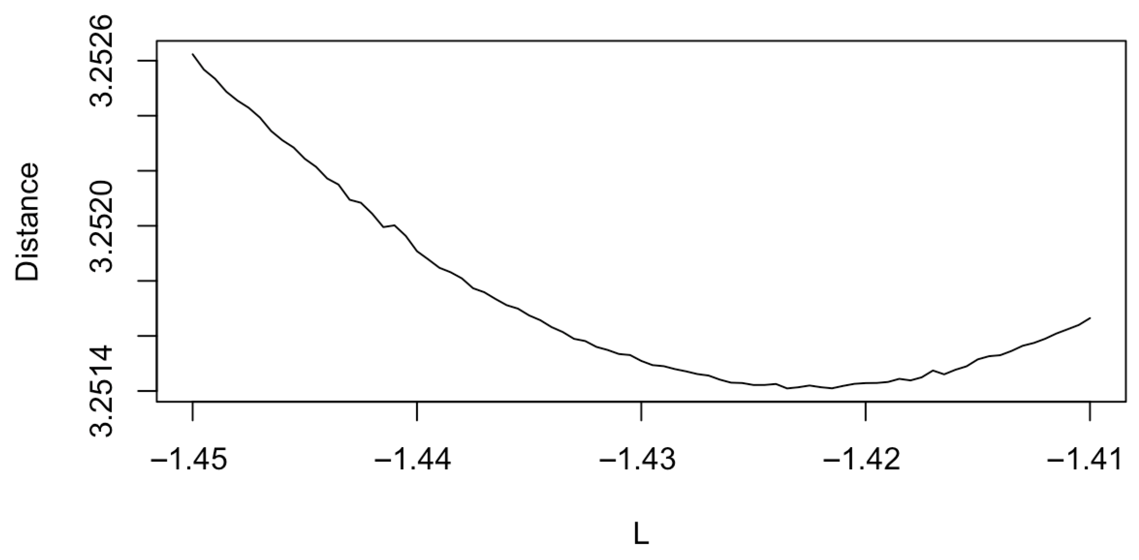
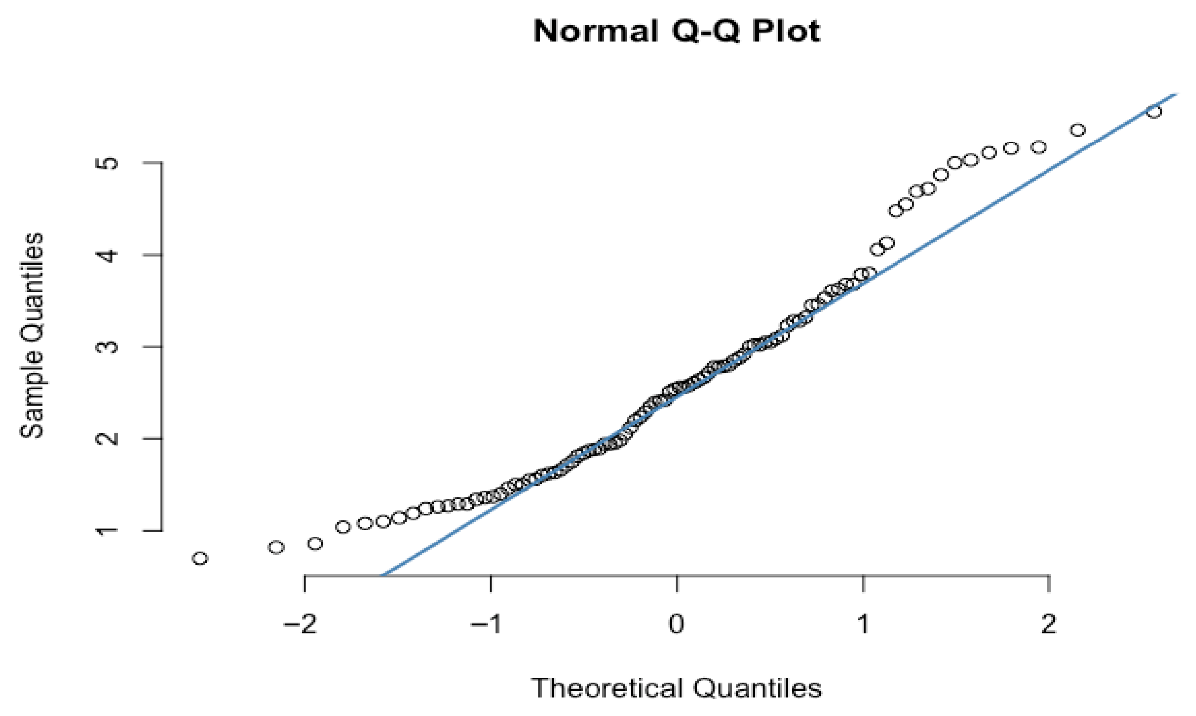
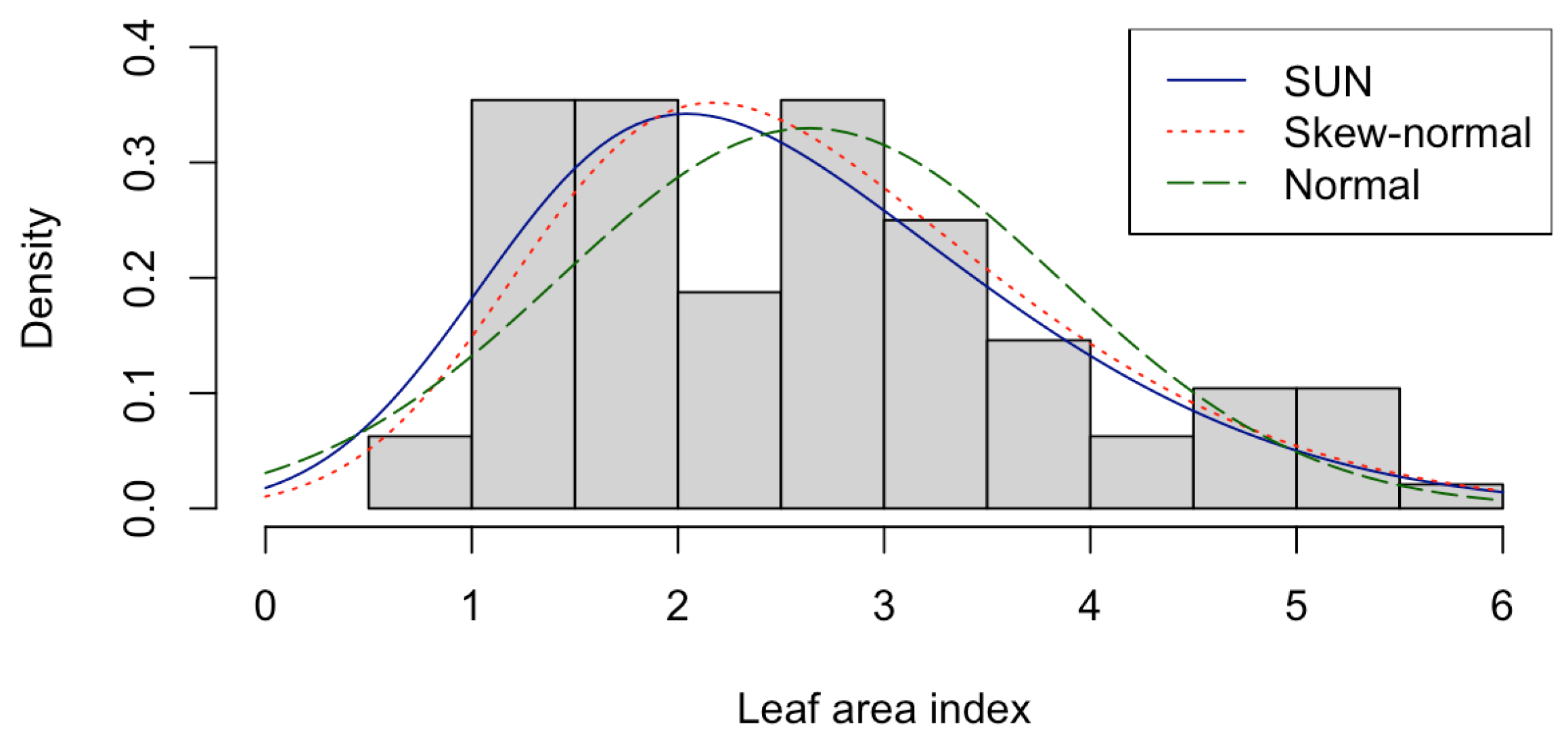
4.1. Leaf Area Index
For the location of the one-sample case, we will use the data set that pertained to the leaf area index (LAI) of Robinia pseudoacacia in the Huaiping Forest Farm of Shaanxi, China, from June to October 2010 provided by Ye and Wang [], with a size of 96. Table 5 presents the comparison among the models with a normal distribution, skew-normal distribution, and SUN distribution by the parameter estimators, the values of the Akaike information criterion (AIC) and Bayesian information criterion (BIC), from which we can see that the SUN has the smallest values in both requirements.
Table 5.
Estimates of the parameters of the normal, skew-normal, and the SUN distributions based on the data set and the corresponding AIC and BIC values.
The Q-Q plot in Figure 8 shows the data to be highly non-normal. The histogram of the data curved by the normal, skew-normal and SUN distributions is given in Figure 9, showing that the SUN fits the data set well.
Figure 8.
The Q-Q plot for the LAI data.
Figure 9.
The histogram of the data of LAI and its SUN-fitted curve.
Given the known population parameters , , , and , we determine the required sample size. For a precision of and a confidence level of , the SUN model yields a required sample size of . In contrast, under the i.i.d. normal assumption—ignoring the asymmetry evident in the normal Q-Q plot (Figure 8) and histogram (Figure 9)—the required sample size is also 11. However, under the skew-normal model incorporating the specific dependence structure proposed by Trafimow et al. [], the required sample size decreases significantly to 5. This reduction occurs because the structured dependence reduces variability. In summary, the APP based on the SUN model accounts for both independence and asymmetry, offering a more comprehensive approach. To construct the 95% confidence interval for under the SUN assumption, we randomly selected a sample of size from the population, obtaining a sample mean . The resulting 95% confidence interval for is , with a length of . The true value lies within this interval.
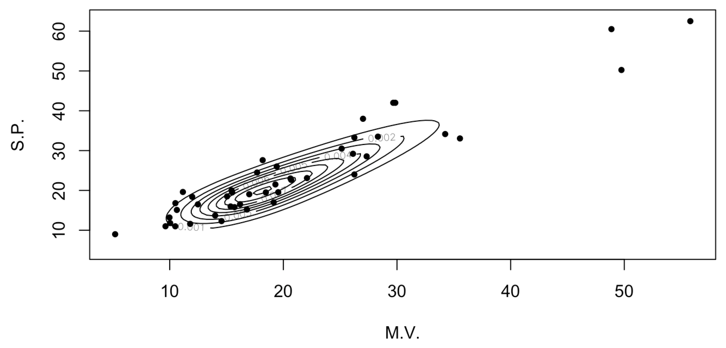
4.2. Sale Price Market Values
In this application, we are going to set up the APP to illustrate the use of the SUN to fit the data from the example given by Wang et al. [], which compares the market values (M.V.) and the selling prices (S.P.) (USD 10,000) of 45 homes. Based on the fact that the family of is similar to the family of -2, which provides a way to estimate parameters in for describing our data, more details can be found in Sahu et al. [] and Arellano-Valle and Azzalini []. The following Figure 10 displays an SUN fitted contour plot of with , ,
Figure 10.
A contour plot fit of the estimated distribution.
Let D be the dependent data set of S.P. and M.V.; then, it follows an SUN distribution, , where , , , and can be obtained by Proposition 4. Let and . The skew-normal fit incorporating the specific dependence structure proposed by Wang et al. [] yields a required sample size of . In contrast, when modeling the data under the i.i.d. normality assumption—ignoring the evident asymmetry shown in Figure 10—the required sample size increases substantially to , reflecting the inefficiency introduced by neglecting this skewness. The SUN model, under the i.i.d. assumption via Theorem 3, requires a sample size of . This approach retains the realistic independent sampling assumption while effectively capturing data skewness, providing a more balanced and broadly applicable solution. We randomly selected a sample of size 16 and calculated the sample mean . The resulting confidence interval for is , which includes the method-of-moments estimate .
5. Discussion
Researchers have primarily focused on developing a priori confidence intervals for the normal distribution, later extending these methods to the more general family of skew-normal distributions, which includes the normal distribution as a special case. However, due to the lack of additive closure under the skew-normal family, the current literature on the adaptive precision procedure (APP) for estimating location parameters assumes that samples jointly follow a multivariate skew-normal distribution. In this framework, individual observations share identical univariate skew-normal marginal distributions but exhibit specific dependencies. This paper addresses a critical gap by providing APP methods to determine the required sample sizes for constructing a priori confidence intervals in three scenarios under the SUN distribution family. The SUN family encompasses the skew-normal distribution as a subset and possesses the crucial property of closure under linear transformations of independent random variables. This extension offers a significant contribution to the field. While our study assumes known scale parameters, related work enhances the broader context. Gupta and Aziz [] introduced weighted moments estimators for SUN populations, which could improve the validity of our findings when scales are unknown. Furthermore, Wang et al. [] developed a Bayesian framework for mixed-type multivariate regression using continuous shrinkage priors. Their approach suggests potential interfaces between Bayesian shrinkage/variable selection methods and our SUN-based APP. To advance this line of research, future study will focus on developing a priori confidence intervals for location parameters in an unknown scale case and differences in locations under the SUN setting when the samples are independent.
Author Contributions
W.T. and C.W.: conceptualization, methodology, validation, investigation, resources, supervision, project administration, visualization, and writing—review and editing; J.Y.: software, formal analysis, and data curation. All authors have read and agreed to the published version of the manuscript.
Funding
The research was supported by the Natural Science Foundation of Top Talent of SZTU (GDRC202214).
Data Availability Statement
The data can be found at the following links: https://doi.org/10.1177/0013164418764801 and https://doi.org/10.1080/03610918.2019.1661473.
Acknowledgments
The authors thank the Academic Editor and three reviewers for their valuable suggestions and modifications, which have improved the quality of this paper.
Conflicts of Interest
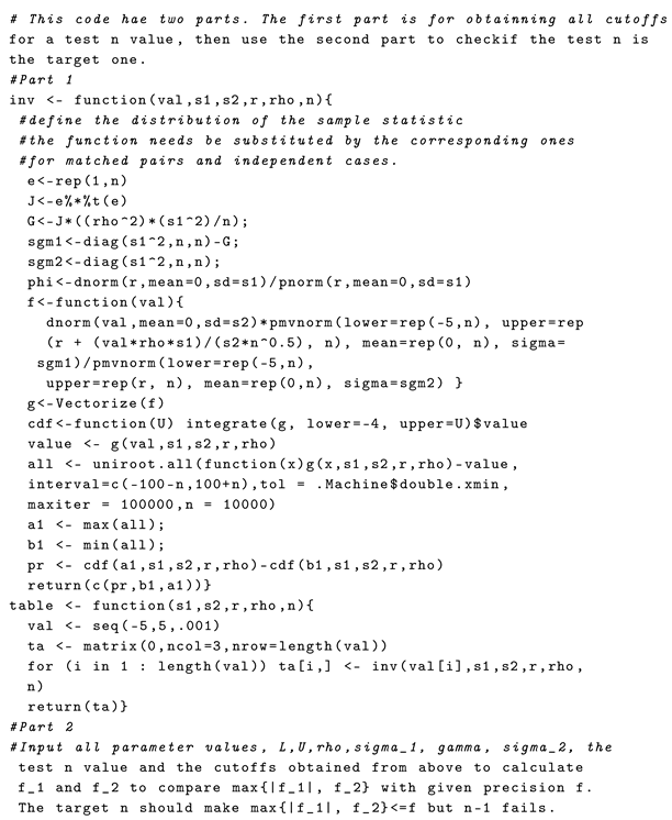
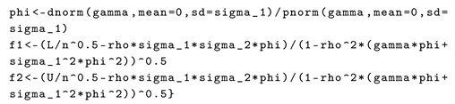
The authors declare no conflicts of interest.
Appendix A
R Code for Calculating the Sample Size Needed With Given Precision and Confidence Level.
| Listing 1. R code for requried sample size. |
![]() |
![]() |
References
- Trafimow, D. Using the coefficient of confidence to make the philosophical switch from a posteriori to a priori inferential statistics. Educ. Psychol. Meas. 2017, 77, 831–854. [Google Scholar] [CrossRef] [PubMed]
- Trafimow, D.; MacDonald, J.A. Performing inferential statistics prior to data collection. Educ. Psychol. Meas. 2017, 77, 204–219. [Google Scholar] [CrossRef] [PubMed]
- Trafimow, D.; Wang, T.; Wang, C. From a sampling precision perspective, skewness is a friend and not an enemy. Educ. Psychol. Meas. 2019, 79, 129–150. [Google Scholar] [CrossRef] [PubMed]
- Azzalini, A.; Dalla Valle, A. The multivariate skew-normal distribution. Biometrica 1996, 83, 715–726. [Google Scholar] [CrossRef]
- Wang, C.; Wang, T.; Trafimow, D.; Chen, J. Extending a priori procedure to two independent samples under skew normal settings. Asian J. Econ. Bank. 2019, 3, 29–40. [Google Scholar]
- Wang, C.; Wang, T.; Trafimow, D.; Myüz, H.A. Necessary sample sizes for specified closeness and confidence of matched data under the skew normal setting. Commun.-Stat.-Simul. Comput. 2022, 51, 2083–2094. [Google Scholar] [CrossRef]
- Ma, Z.; Wang, T.; Choy, S.T.B.; Wei, Z.; Zhu, X. Extending the A Priori Procedure for Estimating Location Parameter Under Multivariate Skew Normal Settings. In Optimal Transport Statistics for Economics and Related Topics; Studies in Systems, Decision and Control; Ngoc Thach, N., Kreinovich, V., Ha, D.T., Trung, N.D., Eds.; Springer: Cham, Switzerland, 2024; Volume 483. [Google Scholar] [CrossRef]
- Tong, T.; Trafimow, D.; Wang, T.; Wang, C.; Hu, L.; Chen, X. The a priori procedure (APP) for estimating regression coefficients in linear models. Methodology 2022, 18, 203–220. [Google Scholar] [CrossRef]
- Cao, L.; Wang, C.; Wang, T.; Trafimow, D. The APP for estimating population proportion based on skew normal approximations and the Beta-Bernoulli process. Commun.-Stat.-Simul. Comput. 2024, 53, 167–177. [Google Scholar] [CrossRef]
- Arellano-Valle, R.B.; Azzalini, A. On the unification of families of skew-normal distributions. Scand. J. Stat. 2006, 33, 561–574. [Google Scholar] [CrossRef]
- Gupta, A.K.; Aziz, M.A.; Ning, W. On some properties of the unified skew normal distribution. J. Stat. Theory Pract. 2013, 7, 480–495. [Google Scholar] [CrossRef]
- Amiri, M.; Jamalizadeh, A.; Towhidi, M. Some multivariate singular unified skew-normal distributions and their application. Commun. -Stat.-Theory Methods 2016, 45, 2159–2171. [Google Scholar] [CrossRef]
- Durante, D. Conjugate Bayes for probit regression via unified skew-normal distributions. Biometrika 2019, 106, 765–779. [Google Scholar] [CrossRef]
- Minozzo, M.; Bagnato, L. A unified skew-normal geostatistical factor model. Environmetrics 2021, 32, e2672. [Google Scholar] [CrossRef]
- Arellano-Valle, R.B.; Azzalini, A. Some properties of the unified skew-normal distribution. Stat. Pap. 2022, 63, 461–487. [Google Scholar] [CrossRef]
- Anceschi, N.; Fasano, A.; Durante, D.; Zanella, G. Bayesian conjugacy in probit, tobit, multinomial probit and extensions: A review and new results. J. Am. Stat. Assoc. 2023, 118, 1451–1469. [Google Scholar] [CrossRef]
- Ye, R.D.; Wang, T.H. Inferences in linear mixed models with skew-normal random effects. Acta Math. Sin. Engl. Ser. 2015, 31, 576–594. [Google Scholar] [CrossRef]
- Sahu, S.K.; Dey, D.K.; Branco, M.D. A new class of multivariate skew distributions with applications to Bayesian regression models. Can. J. Stat. 2003, 31, 129–150. [Google Scholar] [CrossRef]
- Gupta, A.K.; Aziz, M.A. Estimation of Parameters of the Unified Skew Normal Distribution Using the Method of Weighted Moments. J. Stat. Theory Pract. 2012, 6, 402–416. [Google Scholar] [CrossRef]
- Wang, S.-H.; Bai, R.; Huang, H.-H. Two-step mixed-type multivariate Bayesian sparse variable selection with shrinkage priors. Electron. J. Statist. 2025, 19, 397–457. [Google Scholar] [CrossRef]
Disclaimer/Publisher’s Note: The statements, opinions and data contained in all publications are solely those of the individual author(s) and contributor(s) and not of MDPI and/or the editor(s). MDPI and/or the editor(s) disclaim responsibility for any injury to people or property resulting from any ideas, methods, instructions or products referred to in the content. |
© 2025 by the authors. Licensee MDPI, Basel, Switzerland. This article is an open access article distributed under the terms and conditions of the Creative Commons Attribution (CC BY) license (https://creativecommons.org/licenses/by/4.0/).

