Data-Driven Symmetry and Asymmetry Investigation of Vehicle Emissions Using Machine Learning: A Case Study in Spain

Abstract

Understanding vehicle emissions is essential for developing effective carbon reduction strategies in the transport sector. Conventional emission models often assume homogeneity and linearity, overlooking real-world asymmetries that arise from variations in vehicle design and powertrain configurations. This study explores how machine learning and explainable AI techniques can effectively capture both symmetric and asymmetric emission patterns across different vehicle types, thereby contributing to more sustainable transport planning. Addressing a key gap in the existing literature, the study poses the following question: how do structural and behavioral factors contribute to asymmetric emission responses in internal combustion engine vehicles compared to new energy vehicles? Utilizing a large-scale Spanish vehicle registration dataset, the analysis classifies vehicles by powertrain type and applies five supervised learning algorithms to predict CO₂ emissions. SHapley Additive exPlanations (SHAPs) are employed to identify nonlinear and threshold-based relationships between emissions and vehicle characteristics such as fuel consumption, weight, and height. Among the models tested, the Random Forest algorithm achieves the highest predictive accuracy. The findings reveal critical asymmetries in emission behavior, particularly among hybrid vehicles, which challenge the assumption of uniform policy applicability. This study provides both methodological innovation and practical insights for symmetry-aware emission modeling, offering support for more targeted eco-design and policy decisions that align with long-term sustainability goals.

1. Introduction

Transportation has long been a cornerstone of economic development and social connectivity. However, it is now one of the leading contributors to anthropogenic greenhouse gas (GHG) emissions worldwide. The transport sector accounts for approximately 24 percent of direct carbon dioxide (CO₂) emissions from fuel combustion, a figure that is expected to rise further due to ongoing urbanization and motorization [1,2]. Consequently, decarbonizing transportation has become a critical and urgent challenge for advancing sustainable development and enhancing climate resilience [3].

In response to this challenge, European countries, particularly Spain, have implemented a series of transformative policies consistent with the objectives of the European Green Deal [4]. These initiatives promote the integration of vehicle electrification, intelligent mobility systems, fuel efficiency improvements, and renewable energy sources within a unified and sustainable transport framework [5]. The success of these efforts depends not only on technological innovation but also on the capacity to model and analyze vehicle emissions with precision and detail. This requirement is especially important given the structural heterogeneity of modern vehicle fleets, which leads to complex and often asymmetric emission patterns across various powertrain types, usage conditions, and vehicle designs. Conventional emission modeling tools often struggle to account for such real-world complexity and nonlinearity [6].

While laboratory-based testing protocols and simulation models provide useful insights under controlled conditions, they frequently fail to capture the nuanced interactions between vehicle attributes and operational environments. Factors such as dynamic driving behavior, road conditions, and drivetrain architecture can generate asymmetric and nonlinear emission responses that traditional models are not equipped to represent. In contrast, machine learning (ML) techniques offer a flexible, data-driven approach that can uncover hidden patterns in high-dimensional datasets. Advances in explainable artificial intelligence (XAI), especially through the application of SHapley Additive exPlanations (SHAPs), have further improved the interpretability of ML models. These developments enable researchers to identify the specific contributions of individual vehicle characteristics to emission outcomes with greater clarity [7].

Building on this methodological shift, the present study investigates a critical question: how do structural factors drive asymmetric CO₂ emission responses across diverse vehicle categories, particularly between conventional internal combustion engine (ICE) vehicles and new energy vehicles (NEVs)? While previous research has applied ML techniques to emission prediction, these studies have rarely accounted for the non-uniform influence of key features such as fuel consumption, vehicle weight, or hybrid drivetrain configuration. This limitation reduces the practical utility of predictive models in supporting the formulation of performance-based emission policies. By leveraging a comprehensive, high-resolution dataset from the Spanish Institute for Diversification and Energy Saving (IDAE), this study aims to develop an explainable ML framework that not only improves predictive accuracy but also reveals underlying emission asymmetries. The findings offer evidence-based insights to inform symmetry-aware transport policies, challenge the validity of uniform regulatory approaches, and provide a more refined foundation for incentive structures, fleet management strategies, and eco-labeling systems.

The dataset includes detailed vehicle-level information, including engine specifications, physical dimensions, fuel consumption rates, and CO₂ emission values measured under the Worldwide Harmonized Light Vehicles Test Procedure (WLTP). To account for the technological heterogeneity inherent in modern vehicle fleets, the data are categorized into two distinct groups: conventional ICE vehicles powered by petrol or diesel and NEVs, comprising both hybrid and plug-in hybrid vehicles. A total of five supervised ML algorithms are applied to each vehicle group: Multiple Linear Regression (MLR), Random Forest (RF), Gradient Boosting Machines (GBMs), Support Vector Regression (SVR), and K-Nearest Neighbors (KNNs). Model performance is evaluated using four key metrics, namely R-squared (R²), Mean Squared Error (MSE), Root Mean Squared Error (RMSE), and Mean Absolute Error (MAE), to assess their effectiveness in predicting average WLTP CO₂ emissions. Among all models, the RF algorithm consistently demonstrates superior performance, achieving near-perfect R² scores (greater than 0.99) and minimal prediction errors across both the conventional and hybrid vehicle datasets.

To address the opaque nature often associated with ML models, this study incorporates SHAPs to interpret the contribution of individual features to emission outcomes. Rather than focusing solely on predictive accuracy, this approach facilitates the identification of asymmetric and threshold-based relationships across a wide range of vehicle configurations. The results reveal systematic differences in how structural attributes such as fuel consumption, powertrain architecture, and vehicle mass influence emissions. These asymmetries are particularly evident among hybrid vehicle subtypes and across various weight categories, where emission responses deviate substantially from linear or uniform expectations. By emphasizing these nonlinear patterns, the proposed framework enhances model interpretability. It provides a data-driven foundation for advancing vehicle design practices and regulatory standards in support of sustainable transport objectives.

Building on these insights, this study offers a methodological contribution by integrating high-performance ML models with interpretable frameworks such as SHAPs within the context of sustainability analytics. This integration not only enhances predictive accuracy but also enables the identification of hidden structural patterns, particularly in instances where emission responses deviate from assumed symmetry across vehicle attributes or powertrain types. These insights help bridge the gap between algorithmic precision and policy relevance. Policymakers, urban planners, and vehicle manufacturers can apply the findings to prioritize vehicle categories and design specifications that yield the most substantial emission reductions.

In addition, this study emphasizes the value of publicly accessible vehicle registration and emissions datasets as a foundation for evidence-based environmental policymaking. In contexts such as Spain, where climate targets are evolving rapidly, the incorporation of ML into national monitoring systems can enhance both the granularity and responsiveness of transport policies. By uncovering asymmetries and hidden structures within emission data, these analytical tools support more targeted interventions that align with the real-world behavior of vehicles.

In comparison to the existing literature, this study contributes new knowledge in three key areas. First, it combines explainable ML techniques with symmetry-aware analysis to reveal nonlinear and often overlooked emission behaviors. Second, it differentiates emission responses across various hybrid vehicle subtypes, drawing attention to policy-relevant distinctions between plug-in and diesel hybrid systems. Third, it introduces a replicable and scalable modeling framework based on publicly available data, thereby facilitating the translation of interpretable model outputs into actionable transport policy recommendations. These innovations contribute to the broader literature on sustainable transportation and emission modeling, with implications for both academic research and environmental governance.

The remainder of this paper is structured as follows. Section 2 reviews the relevant literature on symmetry-aware emissions modeling and ML applications in sustainable transport. Section 3 describes the dataset, variable selection, and data preprocessing procedures. Section 4 presents the modeling methodology, including the selected algorithms and the SHAP-based interpretation framework. Section 5 discusses empirical results and identifies key drivers of emissions across vehicle categories. Section 6 outlines policy implications and reflects on the observed asymmetries in emission behavior. Finally, Section 7 concludes the paper.

2. Literature Review

2.1. Symmetry and Asymmetry in Traditional Emission Models

Vehicle emission modeling has historically been grounded in linear, proportional relationships, embodying a form of structural symmetry: fuel usage, engine size, or distance travel are assumed to translate directly into emissions. Tools such as COPERT, MOVES, and EMFAC typify this approach, implementing linear emission factors tied to standardized vehicle classes [8,9]. However, accumulating evidence from empirical studies challenges the validity of these symmetrical assumptions, revealing complex and often nonlinear behaviors in emission patterns.

For example, Ciccone and Soldani (2021) conducted a meta-analysis of 50 studies validating various traffic emission models and found consistent asymmetries in prediction accuracy. Their results showed that NO_x emissions are frequently overestimated, while particulate matter (PM) predictions vary widely due to inconsistent measurement definitions. Crucially, the study highlighted that more complex models did not consistently outperform simpler ones, challenging the assumption that increasing model complexity ensures symmetric improvements in accuracy. The authors emphasized the urgent need for models to explicitly quantify uncertainty and establish clear accuracy guidelines, underscoring the pervasive structural asymmetry in current emission modeling practices [10].

Further spatial and structural asymmetries have been documented at the macroeconomic level. Campos-Romero et al. (2024) analyzed the EU28 automotive sector and identified stark differences between Central and Eastern European countries. While Central Europe tends to engage in low-emission, high-value activities, Eastern Europe bears disproportionate environmental burdens from emission-intensive manufacturing. Their findings include an inverted N-shaped Environmental Kuznets Curve that deviates significantly from the classic symmetric inverted U shape. Moreover, increased integration into global value chains was linked to higher emissions, highlighting the need for environmental policies that explicitly recognize and address such asymmetric responsibilities [11]. Using Japan as a case study, Long et al. (2020) examined household private car emissions from 1990 to 2016, highlighting the critical role of individual behavior in decarbonization. While overall emissions declined, spatial analysis revealed that depopulation in certain prefectures was associated with increased car-related emissions. The study underscores the need for regionally targeted decarbonization policies that prioritize demographic characteristics when addressing household transport emissions [12]. A study based on Greece developed aggregate models to forecast CO₂ emissions from cars and buses using socio-economic predictors such as GDP per capita, car occupancy, and bus kilometers. The results showed a sharp increase in car-related emissions, projected to account for 95% of road transport CO₂ emissions by 2010. The study highlights the carbon risks associated with rising private car ownership in lower-income Mediterranean and Eastern European countries with similar socio-economic profiles [13].

Beyond spatial disparities, technological innovation introduces further heterogeneity and asymmetry into emission dynamics. Cheng et al. (2021) used panel quantile regression to demonstrate that innovation reduces CO₂ emissions in OECD countries, but the magnitude and direction of this effect vary significantly across emission levels. The study also showed that innovation asymmetrically moderates the impacts of economic growth and renewable energy adoption, challenging traditional models’ assumption of uniform, symmetric effects [14].

Uncertainties inherent in emission modeling also reveal asymmetric patterns. Kühlwein and Friedrich (2000) assessed the uncertainties in road transport emission estimates and found that accuracy varies considerably by pollutant type, road category, and temporal resolution. They reported substantially higher error margins for urban emissions and cold-start conditions, with variation coefficients reaching up to 100% for heavy-duty vehicles. These results question the assumption of symmetric model performance and underline the critical need to explicitly incorporate and communicate error margins in emission predictions [15].

Longitudinal studies provide further evidence of asymmetric emission trends. McDonald et al. (2013) examined long-term changes in motor vehicle emissions across major US urban areas and found that while CO and NMHC emissions declined substantially due to improved controls, the rates of decline differed by pollutant and vehicle type. Stable NMHC/CO ratios observed in Los Angeles suggest some symmetric control effects; however, divergences in other cities and shifts in CO/NO_x ratios reveal structural asymmetries in emission reductions over time [16]. Xu et al. (2020) developed an energy-based model to quantify passenger car carbon emissions on different highway slopes, incorporating mechanical and thermodynamic principles. Field tests confirmed the model’s high accuracy (max error < 10%). The results showed that average gradient is the dominant factor affecting emissions on continuous slopes, while speed is the key factor on round-trip slopes with mild gradients [17].

Asymmetry is not limited to conventional vehicles. Park et al. (2013) investigated hybrid energy storage systems in electric vehicles (EVs) and highlighted asymmetric energy flows during acceleration and regenerative breaking. They proposed a novel charge migration strategy between batteries and supercapacitors, exploiting these operational asymmetries to improve energy efficiency by 19.4%. This work underscores the importance of managing asymmetric dynamics in hybrid EV energy systems [18].

Finally, fleet-level analyses reveal significant emission inequalities within vehicle populations. Lau et al. (2015) employed plume chasing techniques to assess diesel fleet emissions in Hong Kong and quantified emission inequality using the Gini coefficient. They found that high emitters exist across all vehicle ages and pollutant types, and that vehicles with high emissions of one pollutant are not necessarily high emitters of others. This emission asymmetry emphasizes the importance of multi-pollutant control strategies and targets removal of high emitters, challenging the assumptions behind uniform regulatory frameworks [19].

2.2. Machine Learning and Interpretability: Dissecting Structural Symmetry and Asymmetry

ML techniques have been increasingly employed to predict CO₂ emissions from modern vehicles, particularly full hybrid vehicles, where traditional macroscale emission models often fall short. These conventional models, typically based on symmetric and linear assumptions, are unable to capture the dynamic and heterogeneous characteristics of powertrain behavior. In contrast, ML models provide flexibility to identify nonlinear relationships and asymmetric emission patterns that static, assumption-driven models are not equipped to represent.

For instance, Mądziel et al. (2021) developed an instantaneous CO₂ emission model for full hybrid vehicles using Gaussian process regression trained on Portable Emission Measurement System (PEMS) data. Their approach explicitly captures inherent asymmetries arising from complex factors such as speed, acceleration and road gradient. This allows modeling of real-world nonlinear emission behaviors, including regenerative braking and variable engine loads, which traditional symmetric models overlook [20].

Similarly, Xia et al. (2022) proposed an ML ensemble framework using remote sensing data from over 100,000 gasoline vehicles. Unlike conventional lab tests assuming symmetric conditions, their model reflects the real-world asymmetric emission patterns, enabling continuous and accurate supervision. This demonstrates ML’s advantage in overcoming the static, simplified assumptions of traditional inspection methods [21].

Le Cornec et al. (2020) applied ML to instantaneous NO_x emissions from 70 diesel vehicles, clustering them into 17 groups with similar emission profiles. Their nonlinear regression and neural network models achieved prediction errors below 20%. Importantly, their clustering revealed asymmetric emission behaviors uncorrelated with vehicle characteristics, challenging the uniform emission assumptions of traditional models. The requirement of only speed and acceleration inputs allows rapid, high-resolution emission predictions, providing practical tools for policymakers to address fleet heterogeneity effectively [22].

Further advancing ML applications, Li et al. (2024) developed a deep learning CO₂ emission model using Long Short-Term Memory (LSTM) networks trained on PEMS and GPS data from light-duty diesel trucks. Their model captures asymmetric influences of speed, road slope, and acceleration, notably showing sharp emission increases when acceleration exceeds 5 m/s². Achieving high accuracy (R² up to 0.99), this method surpasses traditional symmetric models by dynamically reflecting context-dependent nonlinear emission behaviors characteristic of real-world transport [23]. Using a large Canadian dataset of over 7000 light-duty vehicles, Natarajan et al. (2023) applied boosting-based regression models to accurately predict CO₂ emissions from vehicle specifications. The models demonstrated strong performance even with minimal input features and offered practical insights for emission reduction strategies [24]. Al-Nefaie and Aldhyani (2023) applied deep learning models to predict vehicle CO₂ emissions using a dataset containing engine specifications, fuel type, and consumption metrics. The BiLSTM model achieved the highest accuracy, outperforming traditional methods [25].

Extending beyond vehicle-level modeling, Peng et al. (2020) developed an intelligent transportation system that integrates ML methods, including genetic algorithms and particle swarm-optimized support vector regression, for traffic flow prediction and dynamic path planning. Their system captures asymmetric traffic conditions and variations in fuel consumption across road networks, enabling adaptive navigation strategies that significantly reduce vehicle CO₂ emissions. This study underscores the importance of incorporating spatial and temporal asymmetries in the design of effective low-carbon transport solutions for smart cities [26].

Xiang et al. (2024) proposed a bi-objective optimization algorithm, MOFECO-SS, for the Green Vehicle-Routing Problem with a symmetric distance matrix, balancing carbon emissions reduction and customer satisfaction. The study demonstrates that leveraging the symmetry inherent in routing distances enhances optimization efficiency and supports environmentally sustainable logistics planning, highlighting the practical benefits of incorporating symmetry principles in transport system design [27].

Udoh et al. (2024) applied regression-based ML models to predict CO₂ emissions from light-duty vehicles using data from the UK Vehicle Certification Agency under WLTP. Among the six models tested, Decision Tree Regression yielded the highest accuracy and was deployed as a web-based real-time emission estimator. By capturing complex, asymmetric variations in emissions data, this approach surpasses traditional static methods that assume symmetry, enabling more dynamic and precise emission assessments critical for sustainable transport policies [28].

Finally, Yin et al. (2024) conducted a comparative analysis of several ML techniques, including decision trees, multinomial logistic regression, multivariate linear regression, and artificial neural networks (ANNs), to forecast greenhouse gas emissions from road transport in China. Their findings indicated that the multilayer perceptron architecture of ANNs outperformed the other models, while ensemble techniques such as bagging and boosting further enhanced predictive accuracy. These ML approaches effectively capture complex, nonlinear, and asymmetric emission patterns, providing robust analytical tools for policymakers seeking to implement data-driven strategies for emission mitigation [29]. To better contextualize the methodological shift,

Table 1. Comparison between traditional emission models and ML-based methods.

Aspect	Traditional Models	ML Methods
Application Scenarios	Standardized lab tests; simulation models	Real-world vehicle emissions with large datasets
Symmetry Assumption	Often assume linear or proportional effects	Allow for nonlinear and asymmetric responses
Input Flexibility	Pre-defined variables with limited scope	Capable of handling high-dimensional features
Interpretability	High (but often based on assumptions)	Limited, but enhanced via SHAP/XAI techniques
Adaptability to Heterogeneity	Poor—struggles with diverse powertrains	Strong—accommodates vehicle-level differences
Limitations	Low real-world validity; rigid assumptions	Potential overfitting; “black box” perception

contrasts traditional emission modeling approaches with ML-based methods in terms of modeling assumptions, input flexibility, and interpretive capability. This structured comparison highlights the limitations of conventional models in capturing asymmetric emission behaviors, thus motivating the data-driven framework adopted in this study.

2.3. Distinctions and Contributions of This Study

While previous studies have demonstrated the utility of ML in predicting vehicle emissions and identifying certain asymmetric patterns, the present study advances the field in four key aspects. First, in contrast to many existing studies that focus on a single vehicle category, such as full hybrids or light-duty gasoline vehicles, or examine a narrow set of pollutants, this study employs a broader, multi-category dataset encompassing ICE vehicles, hybrids, and PHEVs. This comprehensive scope enables a fleet-wide assessment of emission asymmetries across diverse powertrain types. Second, the study assigns equal importance to predictive accuracy and model interpretability. By incorporating SHAPs into the modeling workflow, it offers feature-level insights into the symmetric and asymmetric determinants of emissions, a dimension that has been largely overlooked in previous ML-based emission models. Third, the study extends beyond emission prediction by linking identified asymmetric patterns to policy-relevant implications. In particular, the findings demonstrate how SHAP-based asymmetry analysis can inform differentiated regulatory strategies, including the design of targeted incentives for PHEVs and the implementation of stricter oversight for diesel–hybrid technologies. Fourth, the study enhances existing emission modeling practices by integrating dynamic and structural asymmetry analysis based on real-world, vehicle-level data. As a result, it refines established approaches and illustrates how threshold-driven nonlinearities can support more granular emission forecasting and the development of tailored vehicle policy interventions. In summary, this study offers a comprehensive, interpretable and policy-aligned framework for emission modeling. It bridges methodological advancement with actionable sustainability insights, contributing to both the academic literature on transport emissions and the practical design of carbon mitigation strategies.

3. Data and Variables

3.1. Data Collection

The dataset utilized in this study contains detailed information on fuel consumption and CO₂ emissions for new vehicles registered in Spain as of July 2022. Published by the Spanish government’s IDAE, this dataset aims to enable consumers to compare vehicle fuel efficiency and emissions. The dataset comprises 15,753 observations across 24 variables and is publicly available on the Spanish government’s official website.

Table 2. Variable list.

Variable Name	Description
ID	Identity/unique code
avg_wltp_emissions_gCO2_km	Target variable, average CO2 emissions (g/km) under the WLTP test standard
market_segment	Market segmentation
engine_type	Type of engine: petrol, diesel, plug-in hybrids, petrol hybrids, diesel hybrids, natural gas, LPG
consumption_min_l_100 km	Minimum amount of fuel consumed per 100 km driven
consumption_max_l_100 km	Maximum amount of fuel consumed per 100 km driven
emissions_min_gCO2_km	Minimum amount of CO2 released per kilometer traveled
emissions_max_gCO2_km	Maximum amount of CO2 released per kilometer traveled
transmission	Vehicle transmission method
engine_displacement_cm3	Displacement of the vehicle’s engine in cubic centimeters (cm3)
power_cv	The power of the vehicle’s engine, measured in horsepower (hp)
power_ice_kW	Power of the Internal Combustion Engine (ICE) in kilowatts (kW)
power_electric_kW	Electric power of EVs in kilowatts (kW)
battery_range_km	Battery range of EVs in kilometers (km)
avg_wltp_consumption_l_100 km	Average fuel consumption of vehicles in liters per 100 km driven
length_mm	Length of the vehicle in millimeters (mm)
width_mm	Width of the vehicle in millimeters (mm)
height_mm	Height of the vehicle in millimeters (mm)
gross_vehicle_weight_rating_kg	GVWR in kilograms (kg)
total_seating	Total number of passenger seats accommodated inside the vehicle
fuel_economy_index	Fuel economy index or fuel efficiency index
type_hybrid	Type of hybridization of vehicles
electric_consumption_kWh_100 km	Electric energy consumed per 100 km traveled (kWh)
battery_capacity_kWh	Battery capacity in kilowatt-hours (kWh) carried by EVs

provides a detailed list of the variables:

3.2. Data Exploration and Pre-Processing

Initial data exploration was conducted using descriptive statistics, correlation analysis, and visual inspection to identify potential anomalies, multicollinearity, and structural issues in the dataset. Several steps were made during the pre-processing phase to ensure model robustness and interpretability.

First, vehicles labeled as “Pure electric” were excluded from the analysis, as their operational CO₂ emissions are zero and including them would skew the distribution of the emission variable. Next, features that were either irrelevant to the prediction target or posed risks of data leakage were removed. For example, “max_wltp_emissions_gCO₂_km” and “min_wltp_emissions_gCO₂_km” were excluded, because they are strongly correlated with the target variable “avg_wltp_emissions_gCO₂_km” and including them would compromise model validity by introducing circularity.

Variables with excessive missing data (greater than 80%), such as “ev_motor_kW” (electric motor power) and “ev_range_km” (battery range), were also excluded. The high proportion of missing values made reliable imputation unfeasible, and their inclusion would have introduced instability into the training process. The final feature set was selected to balance information richness with data completeness and model integrity.

Moreover, the original dataset included numerous categorical features in string format, which were transformed into binary variables using one-hot encoding. This encoding approach preserved the nominal nature of the categories, avoided introducing artificial ordinal relationships, and ensured compatibility with the ML models used in this study.

3.3. Dataset Partitioning and Feature Engineering

Due to inherent differences in emission profiles between traditional fuel-powered vehicles and NEVs, the dataset was divided into two subsets for targeted analysis: traditional fuel vehicles (Dataset 1) and NEVs (Dataset 2).

Each subset was partitioned into training (80%) and testing (20%) datasets. The training sets facilitated model development by enabling pattern recognition, while the test sets assessed model predictive performance on unseen data, minimizing overfitting risks.

Feature engineering processes included scaling related emission metrics such as “consumption_min_l_100 km”, “consumption_max_l_100 km”, and “avg_wltp_consumption_l_100 km” to mitigate undue influence on model outcomes. Additionally, redundant or irrelevant variables—such as “power_electric_kW” for diesel or petrol vehicles—were systematically excluded to enhance model relevance and efficiency. Appendix A summarizes key descriptive statistics of selected variables. Notably, the average CO₂ emissions under the WLTP standard were approximately 122 g/km, with a median of 118 g/km. Diesel and petrol engines showed considerable variation in both fuel consumption and emissions. Variables such as vehicle length, weight, and engine displacement also displayed wide ranges, reflecting the wide range of vehicle specifications captured in the dataset.

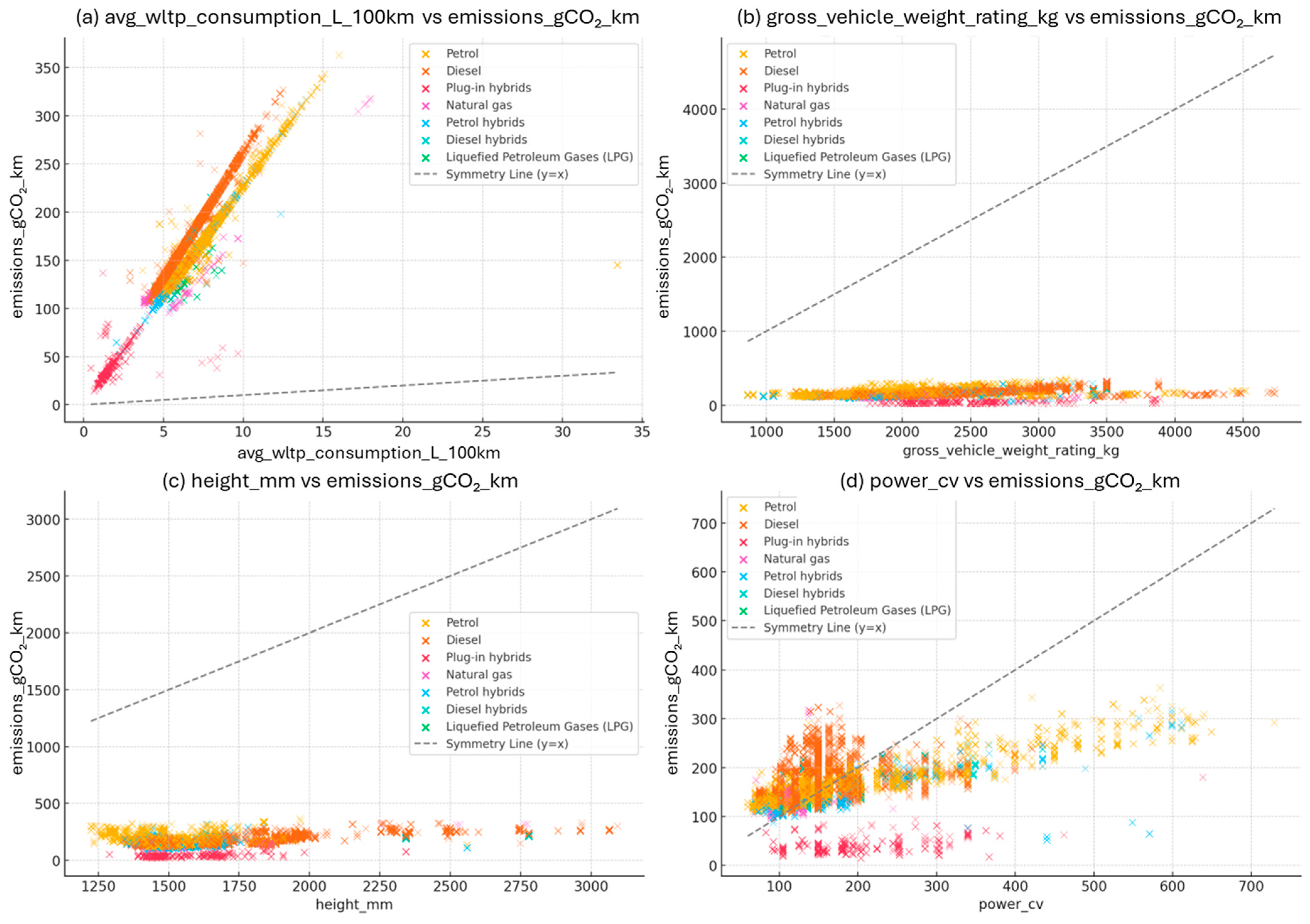
Figure 1 illustrates the associations between selected vehicle attributes and CO₂ emissions, highlighting asymmetric patterns across different engine types. A diagonal reference line (y = x) is included in each subplot to represent hypothetical symmetry; deviations from this line indicate structural or behavioral asymmetries in the underlying data. Panel (a) shows a near-linear correlation between avg_wltp_consumption_l_100 km and emissions; however, the slope and spread varies between petrol and diesel vehicles, implying asymmetric energy conversion efficiencies. Panel (b) reveals that gross vehicle weight rating exerts a nonlinear impact on emissions—vehicles under 1800 kg show limited variation, while heavier vehicles demonstrate a steep increase in emissions, underscoring weight-induced asymmetry. Panel (c) presents vehicle height, where aerodynamic drag effects become increasingly significant beyond 1500 mm, reflecting asymmetrical aerodynamic penalties in taller vehicles. Finally, panel (d) depicts engine power, with asymmetric effects evident across engine categories and power levels; while power generally increases emissions, the rate and magnitude of influence differ notably by engine type.

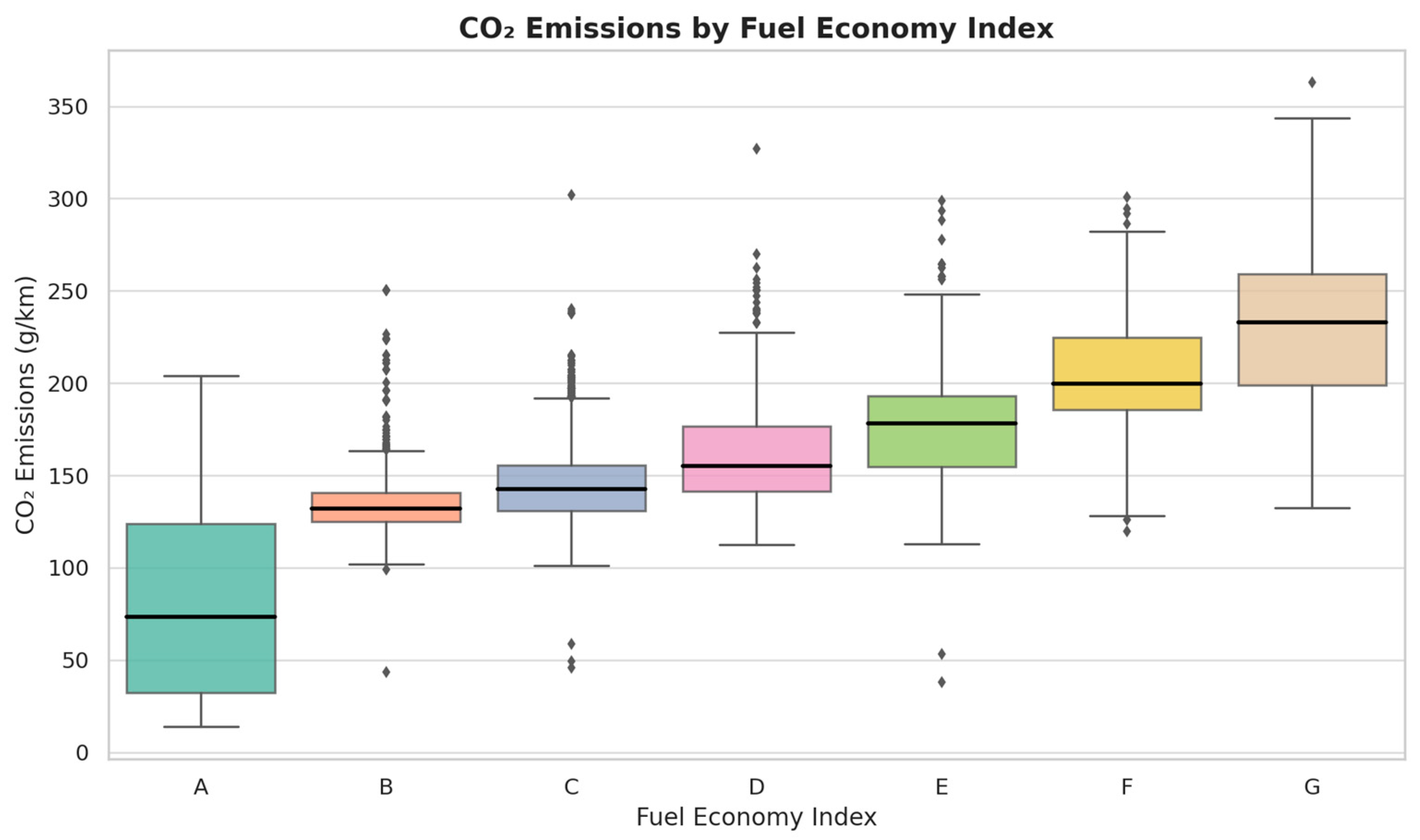
Figure 2 presents the distribution of CO₂ emissions across different fuel economy indices, revealing a form of categorical symmetry. As the rating progresses from A to G, a nearly monotonic increase in median emissions is observed, forming a structurally symmetric profile centered around mid-level categories. This gradient underscores the inverse relationship between fuel efficiency and emissions, supporting the regulatory use of tiered classification systems. Minor asymmetries in dispersion—particularly in extreme categories—highlight the underlying heterogeneity within efficiency classes, inviting further investigation into technological or behavioral factors driving these deviations.

4. Methodology

4.1. Model Development

To explore the relationship between vehicle characteristics and CO₂ emissions, five ML algorithms were employed to construct ten regression models on Datasets 1 and 2. These algorithms include MLR, RF, GBMs, SVR, and KNN. The target variable in all models is the average CO₂ emissions under the WLTP standard (avg_wltp_emissions_gCO₂_km).

MLR is a fundamental statistical technique that assumes a linear relationship between independent variables and the dependent variable. The general form of the model is as follows:

$$Y={\beta }_0+{\beta }_1{X}_1+{\beta }_2{X}_2+\cdots +{\beta }_p{X}_p+ϵ$$

(1)

where $Y$ represents the target variable (average CO₂ emissions); $X_1$ to $X_{\mathrm{p}}$ denote vehicle-related predictor variables (e.g., number of seats, engine power, fuel consumption); ${\beta }_0$ to ${\beta }_p$ are regression coefficients to be estimated; and $ϵ$ is the error term. The model parameters are estimated by minimizing the residual sum of squares, ensuring the best linear unbiased estimators under the Gauss–Markov assumptions [30]. To address potential multicollinearity, Variance Inflation Factor (VIF) analysis was conducted. Features with high VIF values (typically above 10) were removed to stabilize coefficient estimates.

RF is an ensemble learning method based on decision trees. It mitigates the overfitting tendency of single decision trees by averaging predictions from multiple trees trained on bootstrapped samples with random feature selection [31]. The RF regression model predicts as follows:

$${\widehat{Y}}_{RF}={\displaystyle \frac{1}{N_{trees}}}{\sum }_{i=1}^{N_{trees}}{f}_i\left(x\right)$$

(2)

where $f_i\left(x\right)$ is the $i$-th decision tree’s prediction for input $x$. RF handles high-dimensional data well and is robust to noise. Feature importance can be derived by measuring the decrease in MSE or Gini impurity across trees.

GBMs are another ensemble technique, which builds trees sequentially. Each new tree aims to correct the residuals of the previous one by minimizing a differentiable loss function, typically through gradient descent [32]. The predictive function takes the form as follows:

$${\widehat{Y}}_{GBM}\left(x\right)={\sum }_{m=1}^M{\gamma }_m{h}_m\left(x\right)$$

(3)

where $h_m\left(x\right)$ is the $m$-th weak learner (decision tree), and ${\gamma }_m$ is its corresponding learning rate or weight. GBMs are powerful in capturing complex nonlinear interactions but require careful hyperparameter tuning (e.g., number of estimators, learning rate, tree depth) to avoid overfitting. In this study, categorical variables were encoded using one-hot encoding, and grid search combined with 5-fold cross-validation was used for parameter tuning.

SVR extends Support Vector Machines to regression problems by minimizing an insensitive loss function. The regression function in SVR is as below:

$$f\left(x\right)=w^T\varnothing \left(x\right)+b$$

(4)

where $\varnothing \left(x\right)$ maps the input vector into a higher-dimensional space using a kernel function (e.g., radial basis function), and the optimization problem seeks to minimize ${‖w‖}^2$ subject to $ϵ$-precision constraints. SVR is especially effective in high-dimensional spaces and where a sparse solution is desirable [33].

The KNN algorithm is a non-parametric method that makes predictions based on the average target value of the KNN in the feature space. The prediction for a given query point $x$ is as below:

$${\widehat{Y}}_{KNN}\left(x\right)={\displaystyle \frac{1}{k}}{\sum }_{i=1}^k{y}_i$$

(5)

where $y_i$ are the emissions values of the k closest data points to $x$. The KNN algorithm is intuitive and performs well when local patterns dominate the data structure.

Together, these five algorithms cover a spectrum from interpretable linear models to sophisticated nonlinear learners, enabling a robust and diverse assessment of vehicle emission prediction performance.

4.2. Model Evaluation

The performance of each regression model was evaluated using four widely adopted metrics: R², MSE, RMSE, and MAE:

• R²: $R^2=1-{\displaystyle \frac{\sum {{(y}_{i }-{\widehat{ y}}_i)}^2}{\sum {{(y}_i - \overline{y})}^2}}$, representing the proportion of variance in the target explained by the model.
• MSE: $MSE={\displaystyle \frac{1}{n}}\sum {{(y}_i-{\widehat{y}}_i)}^2$, quantifying the average squared prediction error.
• RMSE: $RMSE=\sqrt{MSE}$, allowing direct interpretation in the unit of the target variable.
• MAE: $MAE={\displaystyle \frac{1}{n}}\sum \left|y_i-{\widehat{y}}_i\right|$, measuring the average absolute deviation.

Among these, RMSE was emphasized due to its interpretability and sensitivity to large errors, which is valuable in evaluating emissions-related risk scenarios.

4.3. Model Interpretation

In EV studies, interpretable ML is essential for linking complex data patterns to meaningful engineering and environmental insights [34,35,36]. To interpret the results of the ML models and examine the contribution of each feature, SHAP analysis was applied. SHAP is grounded in cooperative game theory and attributes each feature an importance value for a particular prediction [37].

The SHAP value ${\varnothing }_j$ for feature $j$ is computed as follows:

$${\varnothing }_j=\sum _{S\subseteq N\setminus \left\{j\right\}}{\displaystyle \frac{\left|S\right|!\left(\left|N\right|-\left|S\right|-1\right)!}{\left|N\right|!}}\left(v\left(S\cup \left\{j\right\}\right)-v\left(S\right)\right)$$

(6)

where $N$ is the set of all features; $S$ is a subset of $N$ excluding $j$; and $v\left(S\right)$ is the model output based on features in $S$. This reflects the marginal contribution of feature $j$ averaged over all possible feature subsets.

SHAP values can be integrated into a linear explanation model as below:

$$g\left(z^{’}\right)={\varphi }_0+\sum _{j=1}^M{\varphi }_j{z}_j^{’}$$

(7)

where $g\left(z^{’}\right)$ is the approximated model output; $z_j^{’}$ indicates the presence of feature $j$; and ${\varphi }_j$ is the contribution of that feature. SHAP thus provides global interpretability and local explainability, supporting transparency and trust in model predictions.

Recent advances in EV performance optimization have highlighted the importance of explainable ML models. For example, Liu et al. (2025) introduced a GANDE framework, combining neural decision trees with generalized additive models, demonstrating the value of interpretable ML in electric vehicle applications [38].

The modeling approach adopted in this study is grounded in standard assumptions commonly applied in transport emission prediction. CO₂ emission values are based on certified data published by the Spanish government’s IDAE, which offer a consistent and widely recognized reference for evaluating vehicle-level emissions. These values are assumed to reflect average usage under regulated test conditions, acknowledging that individual driving behaviors and dynamic traffic factors are not captured in the dataset.

The analysis focuses on light-duty vehicles registered in Spain as of 2022, providing policy-relevant insights within a defined national context. Broader temporal or cross-country generalizations are beyond the intended scope of this study. Additionally, the present analysis is limited to tailpipe CO₂ emissions, without considering upstream emissions or full life-cycle impacts, which may be addressed in future work.

5. Results

5.1. Model Performance Comparison

The predictive performance of each algorithm was evaluated separately for two datasets: Dataset 1, consisting of traditional petrol and diesel vehicles, and Dataset 2, comprising hybrid vehicles.

Table 3. Metrics of ML models for Dataset 1.

	MLR	RF	GBT	SVR	KNN
R2	0.999653570	0.9995306	0.9944344	0.994725	0.9487476
MSE	0.048552817	0.9014261	8.568328	8.074402	76.85039
RMSE	0.220347038	0.1592006	2.90826	2.841549	8.766435
MAE	0.19432094	0.9494346	1.252417	1.940012	4.176998

and

Table 4. Metrics of ML models for Dataset 2.

	MLR	RF	GBT	SVR	KNN
R2	0.9425808	0.9995306	0.9822744	0.9835183	0.8663517
MSE	6.27365001	4.399797	49.65703	48.70634	375.3073
RMSE	2.504725536	0.4489223	7.035858	6.978993	19.37285
MAE	2.504725536	2.097569	2.839992	3.356731	6.992

summarize the R², MSE, RMSE, and MAE values for the five regression models applied to each dataset.

For Dataset 1 (petrol and diesel vehicles), ensemble learning models, particularly RF, demonstrated exceptional predictive accuracy. RF achieved the lowest RMSE (0.1592) and a high R² (0.9995), indicating that over 99.95% of the variation in CO₂ emissions was explained by the model with minimal residual error. Similarly, GBT and SVR yielded strong performance, both with R² values exceeding 0.994, and RMSE values below 3.0, suggesting excellent generalization capacity.

MLR also performed well (R² = 0.9996; RMSE = 0.2203), despite being the most interpretable yet assumption-restricted model. In contrast, the KNN model recorded the weakest performance, with an RMSE of 8.77 and a lower R² value of 0.9487, reflecting inferior ability to capture complex relationships in traditional fuel vehicle data.

For Dataset 2 (hybrid vehicles), the RF model again outperformed all others, attaining the highest R² value (0.9995) and the lowest RMSE (0.4489), showcasing its robustness across different vehicle types. GBT also produced competitive results, with an R² = 0.9823 and the RMSE = 7.04, though it exhibited slightly higher error levels compared to RF. MLR maintained reasonable explanatory power (R² = 0.9426) but was less effective in minimizing prediction error (RMSE = 2.50), likely due to the more complex nonlinear structure of hybrid vehicle data. Both SVR and KNN performed relatively poorly, with higher RMSEs (6.98 and 19.37, respectively) and lower R² values, indicating reduced model fit and generalization ability.

These findings collectively indicate that ensemble-based algorithms, particularly RF and GBT, are highly effective in capturing the nonlinear, high-dimensional, and structurally heterogeneous relationships that characterize real-world vehicle emissions data. Their ability to model complex feature interactions and accommodate asymmetric response patterns renders them especially suitable for producing robust and interpretable emissions forecasts.

5.2. Random Forest Feature Importance Interpretation

5.2.1. Traditional Fuel Vehicles

Figure 3 presents the SHAP summary plot of the RF model trained on Dataset 1, highlighting the top 20 features influencing CO₂ emissions from diesel and gasoline vehicles. Among them, the five most impactful variables are consumption_l_100 km, avg_wltp_consumption_l_100 km, engine_type, gross_vehicle_weight_rating_kg, and height_mm.

These features exhibit not only high SHAP magnitudes but also consistent directionality, indicating stable and robust contributions to the model’s predictions. The dominance of consumption-related variables underscores the strong and direct relationship between fuel use and emissions, while structural factors such as vehicle mass and height further reinforce the importance of physical design characteristics.

5.2.2. Hybrid Vehicles (Dataset 2)

Figure 4 displays the SHAP summary plot for the hybrid vehicle dataset (Dataset 2). The most influential features in this model are: avg_wltp_consumption_l_100 km, consumption_l_100 km, engine_type_Plug-in hybrids, engine_type_Diesel hybrids, and gross_vehicle_weight_rating_kg.

Compared to Dataset 1, where conventional vehicles exhibit relatively symmetrical and consistent feature effects, the hybrid dataset reveals greater structural heterogeneity. Specifically, engine type plays a more differentiated role: plug-in and diesel hybrids emerge as distinct predictors, with opposing SHAP contributions. This shift marks a departure from the symmetrical emission patterns observed in traditional vehicles, highlighting the asymmetric influence of hybrid powertrain configurations.

Nonetheless, fuel consumption metrics (avg_wltp_consumption_l_100 km and consumption_l_100 km) and gross vehicle weight remain key predictors across both datasets, reaffirming their universal relevance in emissions modeling despite variation in powertrain architecture.

5.3. Multiple Linear Regression Analysis

5.3.1. Traditional Fuel Vehicles (Dataset 1)

The linear regression results for Dataset 1 are summarized in

Table 5. Coefficient table and significance test for MLR on Dataset 1.

Variable	Estimate	Std. Error	t value	Pr(>|t|)	Signif.
(Intercept)	0.1898	0.1564	1.214	0.2249
consumption_l_100 km	23.15	0.04969	474.4	2 × 10−16	***
engine_displacement_cm3	5.938 × 10−5	1.435 × 10−5	4.139	3.5 × 10−5	***
power_cv	0.003417	0.000878	3.893	9.92 × 10−5	***
power_ice_kW	0.004537	0.001411	3.214	0.00131	**
avg_wltp_consumption_l_100 km	−23.54	0.08689	−271.2	2 × 10−16	***
avg_wltp_emissions_gCO2_km	−0.07721	0.0002846	−271.2	2 × 10−16	***
length_mm	−5.489 × 10−5	1.896 × 10−5	−2.903	0.003679	**
width_mm	3.473 × 10−5	1.843 × 10−5	1.884	0.05975	.
height_mm	−1.348 × 10−5	1.519 × 10−5	−0.887	0.3759
gross_vehicle_weight_rating_kg	−0.0001482	1.815 × 10−5	−8.164	3.89 × 10−16	***
total_seating	−0.07725	0.04	−1.931	0.05349	.
transmissionA	−0.1254	0.1418	−0.884	0.3768
transmissionM	−0.01978	0.01268	−1.561	0.1181
fuel_economy_indexA	0.7753	0.02381	32.56	2 × 10−16	***
fuel_economy_indexB	0.6128	0.0241	25.43	2 × 10−16	***
fuel_economy_indexC	0.5045	0.02407	20.96	2 × 10−16	***
fuel_economy_indexD	0.1972	0.02392	8.246	2 × 10−16	***
fuel_economy_indexE	0.19	0.02491	7.628	2.44 × 10−14	***
fuel_economy_indexF	−0.0634	0.02499	−2.537	0.01118	*
fuel_economy_indexG	−0.06819	0.02878	−2.369	0.01783	*

***: p < 0.001; **: p < 0.01; *: p < 0.05; .: p < 0.1.

, with an adjusted R² of 0.9997, indicating an excellent model fit.

Several predictors show strong and statistically significant associations with emissions (p < 0.001). Positively correlated variables include consumption_l_100 km, height_mm, engine_displacement_cm³, and avg_wltp_emissions_gCO₂_km, while avg_wltp_consumption_l_100 km and multiple fuel economy index categories (C, D, and F) exhibit significant negative correlations.

These results reinforce the SHAP-based findings, suggesting a structurally symmetric pattern in traditional vehicles: fuel consumption and size-related variables consistently increase emissions, while higher fuel economy classes are associated with reductions. The presence of clear directionality and stable effect magnitudes across variables reflects a regular and interpretable emission structure, well captured by linear modeling.

5.3.2. Hybrid Vehicles (Dataset 2)

The MLR model fitted on the hybrid vehicle dataset (Dataset 2) demonstrates relatively strong explanatory power, with an adjusted R² value of 0.9425 (

Table 6. Coefficient table and significance test for MLR on Dataset 2.

Variable	Estimate	Std. Error	t Value	Pr(>|t|)	Signif.
(Intercept)	−71.82	4.968	−14.458	<2 × 10−16	***
consumption_l_100 km	18.19	0.09698	187.582	<2 × 10−16	***
engine_displacement_cm3	0.00185	0.0002567	7.208	6.13 × 10−13	***
power_cv	−0.1341	0.01175	−11.415	<2 × 10−16	***
power_ice_kW	0.1247	0.01555	8.019	1.20 × 10−15	***
length_mm	0.006641	0.0008201	8.098	6.30 × 10−16	***
width_mm	0.02968	0.002715	10.933	<2 × 10−16	***
height_mm	−0.008549	0.001062	−8.049	<2 × 10−16	***
gross_vehicle_weight_rating_kg	0.002145	0.000612	3.504	0.000460	***
total_seating	1.364	0.2265	6.021	1.73 × 10−9	***
transmissionA	0.4953	0.231	2.144	0.032023	*
transmissionM	0.7783	0.2332	3.337	0.000849	***
fuel_economy_indexA	−8.823	0.588	−15.082	<2 × 10−16	***
fuel_economy_indexB	−6.563	0.542	−12.114	<2 × 10−16	***
fuel_economy_indexC	−5.016	0.4441	−11.296	<2 × 10−16	***
fuel_economy_indexD	−2.647	0.6672	−3.966	<2 × 10−16	***
fuel_economy_indexE	−2.066	0.481	−4.296	<2 × 10−16	***
fuel_economy_indexF	37.22	11.6	3.209	0.00134	**
fuel_economy_indexG	40.22	2.019	19.925	<2 × 10−16	***

***: p < 0.001; **: p < 0.01; *: p < 0.05.

). Several variables exhibit statistically significant negative associations with CO₂ emissions, including power_cv, height_mm, and fuel_economy_indexA (p < 0.001), which aligns with expectations that more compact, lightweight, and energy-efficient hybrid configurations tend to generate lower emissions. In contrast, traditional engine-related variables such as consumption_l_100 km, power_ice_kW, and engine_displacement_cm³ show strong positive correlations with emissions, reaffirming their continued operational relevance even within hybrid powertrain systems.

Notably, unlike the consistent directionality observed in conventional vehicles, the hybrid dataset reveals a more mixed pattern of influence, reflecting asymmetries in how structural and powertrain variables interact under varying degrees of electrification. This divergence underscores the need for drivetrain-specific modeling strategies and challenges the assumption of uniform emission behavior across hybrid types.

6. Discussion

6.1. Traditional Fuel Vehicles (Dataset 1)

Figure 5 presents SHAP dependence plots for the five most influential features affecting CO₂ emissions in conventional vehicles: consumption_l_100 km, avg_wltp_consumption_l_100 km, engine_type, gross_vehicle_weight_rating_kg (GVWR), and height_mm. These plots offer insights not only into the magnitude of each variable’s contribution but also into its directionality and the presence of nonlinear thresholds. This allows for the identification of structured relationships that may be overlooked by linear models. The emergence of such consistent patterns suggests a relatively symmetric emission response, in which variations in physical attributes result in proportionate and interpretable changes in emission levels.

Fuel consumption per 100 km (consumption_l_100 km) is identified as the most influential predictor. SHAP analysis reveals a distinct breakpoint at approximately 6.5 L/100 km. Below this level, marginal increases in fuel consumption are associated with relatively modest changes in CO₂ emissions. However, beyond this point, SHAP values increase sharply, indicating a nonlinear and asymmetric escalation. This threshold likely reflects the compounded inefficiencies present in higher-consumption vehicles. When fuel consumption exceeds 6.5 L/100 km, internal combustion engines tend to operate further from their thermodynamic optimal load, and energy losses due to engine friction, idling, and suboptimal transmission ratios increase disproportionately. Additionally, vehicles in this range often have heavier chassis and less aerodynamic designs, which further elevate CO₂ emissions per kilometer. From a regulatory standpoint, this threshold represents a technically grounded inflection point for designing policy instruments. For instance, fuel economy standards or tiered taxation schemes could be structured to increase sharply beyond this level, thereby internalizing the external costs associated with disproportionately high emissions. In contrast to flat thresholds, such an approach more accurately reflects real-world emission behavior and establishes a steeper incentive gradient for efficiency improvements just above the 6.5 L/100 km mark.

Avg_wltp_consumption_l_100 km, which captures standardized fuel use under the WLTP protocol, exhibits a similarly strong and monotonic relationship. As the WLTP test simulates a broad range of driving conditions (e.g., acceleration, idling, and deceleration), this variable serves as a robust proxy for average efficiency. The convergence in SHAP profiles between real-world and standardized consumption measures underscores a structural symmetry in how combustion efficiency translates into carbon output across driving contexts.

The variable engine_type (coded as 0 for diesel and 1 for petrol) provides additional explanatory value. Diesel engines consistently exhibit higher SHAP values, indicating a stronger positive contribution to predicted CO₂ emissions. This observation is consistent with engineering evidence: although diesel engines are generally more thermally efficient, they combust fuel with higher carbon density and typically produce greater quantities of CO₂, NO_x, and PM. While modern diesel vehicles are equipped with after-treatment systems to mitigate these emissions, such technologies are not always sufficient to offset the inherent asymmetries in pollutant output when compared to petrol engines. These findings point to a structural imbalance in emission potential between fuel types, with diesel vehicles exhibiting systematically higher emission contributions.

Gross Vehicle Weight Rating (GVWR) contributes to emissions through its impact on propulsion energy demand. The SHAP plot shows a piecewise effect: below 2500 kg, GVWR has limited influence; beyond this threshold, its contribution increases sharply, indicating a nonlinear amplification of emissions as vehicle mass increases. This effect likely arises from drivetrain inefficiencies, higher rolling resistance and aerodynamic penalties in heavier vehicles. The presence of a distinct threshold again reflects partial symmetry, where structural variables have stable effects up to a point and then diverge.

Height_mm, representing vehicle height, affects emissions through its influence on aerodynamic drag, center of gravity, and suspension design. The SHAP dependence plot shows a general upward trend, with the steepest increase occurring between 1500 mm and 1750 mm. This suggests that this range is particularly critical for aerodynamic inefficiencies. Beyond 2000 mm, SHAP values tend to level off, indicating a saturation effect. This plateau may reflect a diminishing marginal penalty once the vehicle’s shape, load, or function, such as the distinction between SUVs and vans, becomes the dominant factor in aerodynamic performance.

In summary, the SHAP dependence plots reveal a structured and interpretable emissions landscape for conventional vehicles, where most physical and combustion-related features display directionally consistent and often threshold-based effects. This overall symmetry in the relationships between features and emissions supports the application of both linear and ensemble-based machine learning models in this context. It also provides a strong foundation for the development of threshold-sensitive emission policies, eco-design strategies, and targeted public guidance measures.

6.2. Hybrid Vehicles (Dataset 2)

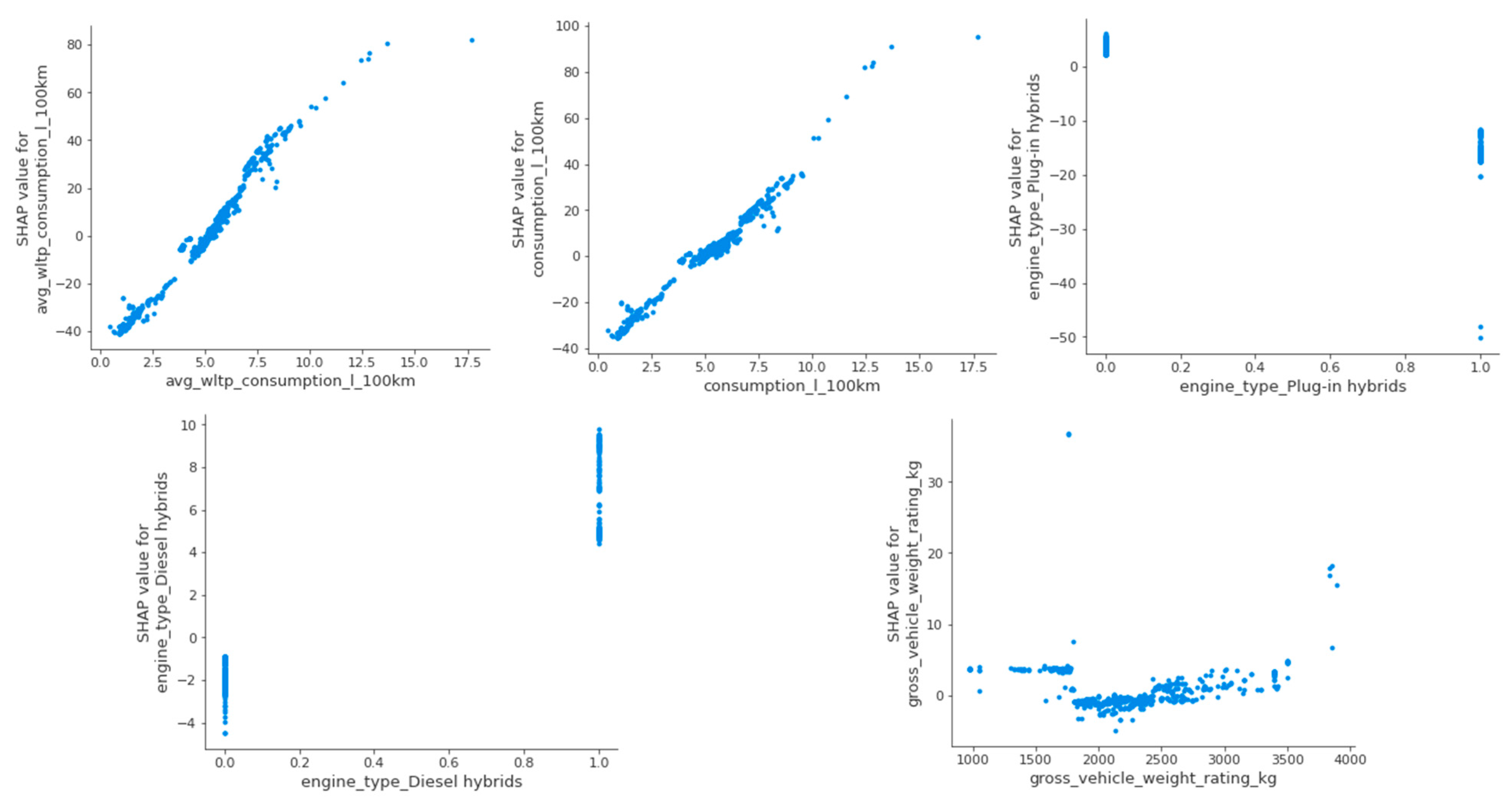
Figure 6 presents SHAP dependence plots for five key variables influencing CO₂ emissions in hybrid and NEVs: avg_wltp_consumption_l_100 km, consumption_l_100 km, engine_type_Plug-in hybrids, engine_type_Diesel hybrids, and gross_vehicle_weight_rating_kg (GVWR). These plots illustrate how electrified powertrains interact with traditional fuel consumption patterns and structural design, revealing notable asymmetries and nonlinearities in emission responses.

Fuel consumption remains the dominant driver of emissions, even in hybrid configurations. Both avg_wltp_consumption_l_100 km and consumption_l_100 km display near-linear and strongly positive SHAP trends, confirming that higher fuel usage results in proportionally greater emissions under both standard and real-world driving conditions. However, in contrast to the case of conventional vehicles, where the SHAP plots indicated a distinct threshold near 6.5 L/100 km, the hybrid vehicle plots exhibit smoother gradients. This suggests a more elastic and less abrupt emission response. The observed pattern reflects the partial substitution effect provided by electric propulsion, which reduces but does not eliminate fuel-based emissions.

The asymmetry between PHEVs and diesel hybrids stems from fundamental differences in powertrain architecture and fuel characteristics. PHEVs are equipped with larger batteries and onboard charging systems, which enable substantial electric-only driving. This feature is particularly effective in urban environments. Their hybrid control strategies are designed to prioritize electric propulsion whenever feasible, often relegating ICE usage to a secondary role. In contrast, most diesel hybrids employ mild or parallel hybrid systems with limited electric range and smaller battery capacities. These vehicles lack plug-in capabilities and rely heavily on the diesel engine, which emits more CO₂ per liter of fuel compared to petrol. Moreover, diesel engines tend to perform inefficiently in stop-and-go traffic conditions, where hybridization offers minimal benefits. These structural and operational limitations account for the higher emissions observed in diesel hybrids relative to PHEVs, despite both being categorized under the general label of “hybrid” vehicles. The findings are consistent with recent studies by Guo et al. (2024) and Alam et al. (2025) and further contribute to the literature by differentiating among hybrid subtypes. This differentiation demonstrates that not all hybrid configurations deliver equivalent environmental benefits [39,40].

The SHAP plot for GVWR further supports the observation of conditional asymmetry. For hybrid vehicles weighing less than 1800 kg, vehicle mass exerts minimal influence on CO₂ emissions. This suggests that other factors, such as the ratio of battery capacity to engine size and engine control strategies, play a more dominant role. However, beyond this threshold, SHAP values begin to increase, indicating that structural mass becomes more significant in heavier hybrid models. This nonlinear transition points to an inflection zone in which battery expansion and structural reinforcements lead to diminishing returns in emission reduction. This pattern is particularly evident in sport utility vehicles and performance-focused hybrid configurations.

Overall, the SHAP analysis for Dataset 2 reveals a less uniform and more segmented emission landscape compared to traditional fuel vehicles. Fuel consumption remains central, but its effects are moderated by drivetrain design and electric power integration. The divergence in SHAP responses across hybrid types emphasizes the need for drivetrain-aware emission policy, where not all “hybrids” are treated equally. Plug-in hybrids emerge as viable transitional solutions, while diesel hybrids demand closer scrutiny. These findings also reinforce the importance of structural weight management in hybrid vehicle design, especially as energy storage needs increase.

In summary, while conventional vehicles display relatively symmetric and consistent emission responses across key features, hybrid vehicles introduce nonlinearities and asymmetries that challenge the effectiveness of uniform regulatory strategies. These nuanced response patterns highlight the value of explainable machine learning tools in supporting targeted and evidence-based decarbonization pathways for the future of transport systems.

7. Conclusions

This study proposes an interpretable ML framework for predicting CO₂ emissions from newly registered vehicles in Spain, incorporating both ICE vehicles and NEVs. Among the five supervised learning algorithms evaluated, ensemble-based models, particularly the Random Forest algorithm, demonstrated the highest levels of predictive accuracy and robustness.

A key contribution of this study is the integration of SHAP to identify asymmetric and threshold-based relationships between vehicle characteristics and CO₂ emissions. Fuel consumption emerged as the most dominant and symmetric predictor, with both real-world and standardized measures (consumption_L/100 km and avg_WLTP_consumption_L/100 km) displaying strong positive SHAP responses. Notably, emissions increased disproportionately beyond the 6.5 L/100 km threshold, indicating that regulatory limits on fuel consumption may lead to substantial reductions in emissions.

The results also reveal significant asymmetries across hybrid subtypes. PHEVs consistently exhibited negative SHAP values, confirming their capacity to reduce emissions under typical driving conditions. In contrast, diesel hybrids contributed positively to predicted emissions, suggesting limited environmental benefits despite the presence of hybrid technology. These findings highlight the need for performance-based incentive schemes that account for actual environmental outcomes, rather than relying on technology-neutral classifications.

GVWR exhibited a nonlinear effect on emissions, particularly among hybrid vehicles. While vehicles weighing less than 1800 kg showed relatively stable emission levels, heavier models displayed a clear upward trend. This pattern supports the implementation of weight-sensitive design incentives, such as taxation measures or credits for the use of lightweight materials.

Overall, this study presents a replicable, interpretable, and symmetry-aware approach to vehicle emission modeling. The findings support the development of more nuanced transport policies that move beyond binary classifications, such as ICE versus hybrid, and instead acknowledge the varied emission profiles across different vehicle categories. Tiered emission caps, dynamic registration fees based on predicted emissions, and structurally targeted incentives represent some of the policy instruments that can be informed by this modeling framework.

As countries such as Spain advance toward their 2030 and 2050 climate targets, the application of interpretable artificial intelligence methods in conjunction with high-resolution vehicle-level data offers a promising pathway to bridge the gap between scientific modeling and policy implementation. By capturing both generalizable patterns and asymmetric emission behaviors, this approach contributes meaningfully to sustainable and adaptive transport governance. Beyond national relevance, this research aligns with several United Nations Sustainable Development Goals (SDGs). By enhancing the modeling of vehicle emissions and revealing asymmetric response patterns, the findings support SDG 11 (Sustainable Cities and Communities) through the facilitation of more effective low-emission urban transport planning. The analysis also advances SDG 12 (Responsible Consumption and Production) by enabling better-informed decisions among consumers and manufacturers, grounded in structural efficiency. Most notably, the study supports SDG 13 (Climate Action) by offering policy-relevant insights into targeted decarbonization strategies, particularly through a more nuanced treatment of hybrid vehicle categories and weight-related thresholds. The proposed framework, therefore, serves as a bridge between data-driven innovation and global sustainability objectives.

References

1. Henke, I.; Cartenì, A.; Beatrice, C.; Di Domenico, D.; Marzano, V.; Patella, S.M.; Picone, M.; Tocchi, D.; Cascetta, E. Fit for 2030? Possible scenarios of road transport demand, energy consumption and greenhouse gas emissions for Italy. Transp. Policy 2024, 159, 67–82. [Google Scholar] [CrossRef]
2. Asim, M.; Usman, M.; Abbasi, M.S.; Ahmad, S.; Mujtaba, M.A.; Soudagar, M.E.M.; Mohamed, A. Estimating the long-term effects of national and international sustainable transport policies on energy consumption and emissions of road transport sector of Pakistan. Sustainability 2022, 14, 5732. [Google Scholar] [CrossRef]
3. Nordin, I.; Elofsson, K.; Jansson, T. Cost-effective reductions in greenhouse gas emissions: Reducing fuel consumption or replacing fossil fuels with biofuels. Energy Policy 2024, 190, 114138. [Google Scholar] [CrossRef]
4. Delbeke, J. Delivering a Climate Neutral Europe; Taylor & Francis; Routledge: Oxfordshire, UK, 2024; p. 297. [Google Scholar]
5. Wang, J.; Zhang, H.; Wu, B.; Liu, W. Symmetry-Guided Electric Vehicles Energy Consumption Optimization Based on Driver Behavior and Environmental Factors: A Reinforcement Learning Approach. Symmetry 2025, 17, 930. [Google Scholar] [CrossRef]
6. Ruiz, E.; Yushimito, W.F.; Aburto, L.; de la Cruz, R. Predicting passenger satisfaction in public transportation using machine learning models. Transp. Res. Part A Policy Pract. 2024, 181, 103995. [Google Scholar] [CrossRef]
7. Peng, Q.; McKillop, D.; Quinn, B.; Liu, K. Modeling and predicting failure in US credit unions. Int. J. Forecast. 2025, 41, 1237–1259. [Google Scholar] [CrossRef]
8. Li, F.; Zhuang, J.; Cheng, X.; Li, M.; Wang, J.; Yan, Z. Investigation and prediction of heavy-duty diesel passenger bus emissions in Hainan using a COPERT model. Atmosphere 2019, 10, 106. [Google Scholar] [CrossRef]
9. Ma, S.; Tong, D.; Harkins, C.; McDonald, B.C.; Wang, C.T.; Li, Y.; Baek, B.H.; Woo, J.; Zhang, Y. Impacts of on-road vehicular emissions on US air quality: A comparison of two mobile emission models (MOVES and FIVE). J. Geophys. Res. Atmos. 2024, 129, e2024JD041494. [Google Scholar] [CrossRef]
10. Ciccone, A.; Soldani, E. Stick or carrot? Asymmetric responses to vehicle registration taxes in Norway. Environ. Resour. Econ. 2021, 80, 59–94. [Google Scholar] [CrossRef]
11. Campos-Romero, H.; Rodil-Marzábal, Ó.; Pérez, A.L.G. Environmental asymmetries in global value chains: The case of the European automotive sector. J. Clean. Prod. 2024, 449, 141606. [Google Scholar] [CrossRef]
12. Long, Y.; Huang, D.; Lei, T.; Zhang, H.; Wang, D.; Yoshida, Y. Spatiotemporal variation and determinants of carbon emissions generated by household private car. Transp. Res. Part D Transp. Environ. 2020, 87, 102490. [Google Scholar] [CrossRef]
13. Paravantis, J.A.; Georgakellos, D.A. Trends in energy consumption and carbon dioxide emissions of passenger cars and buses. Technol. Forecast. Soc. Change 2007, 74, 682–707. [Google Scholar] [CrossRef]
14. Cheng, C.; Ren, X.; Dong, K.; Dong, X.; Wang, Z. How does technological innovation mitigate CO2 emissions in OECD countries? Heterogeneous analysis using panel quantile regression. J. Environ. Manag. 2021, 280, 111818. [Google Scholar] [CrossRef]
15. Kühlwein, J.; Friedrich, R. Uncertainties of modelling emissions from road transport. Atmos. Environ. 2000, 34, 4603–4610. [Google Scholar] [CrossRef]
16. McDonald, B.C.; Gentner, D.R.; Goldstein, A.H.; Harley, R.A. Long-term trends in motor vehicle emissions in US urban areas. Environ. Sci. Technol. 2013, 47, 10022–10031. [Google Scholar] [CrossRef]
17. Xu, J.; Dong, Y.; Yan, M. A model for estimating passenger-car carbon emissions that accounts for uphill, downhill and flat roads. Sustainability 2020, 12, 2028. [Google Scholar] [CrossRef]
18. Park, S.; Kim, Y.; Chang, N. Hybrid energy storage systems and battery management for electric vehicles. In Proceedings of the 50th Annual Design Automation Conference, Austin, TX, USA, 2–6 June 2013; pp. 1–6. [Google Scholar]
19. Lau, C.F.; Rakowska, A.; Townsend, T.; Brimblecombe, P.; Chan, T.L.; Yam, Y.S.; Močnik, G.; Ning, Z. Evaluation of diesel fleet emissions and control policies from plume chasing measurements of on-road vehicles. Atmos. Environ. 2015, 122, 171–182. [Google Scholar] [CrossRef]
20. Mądziel, M.; Jaworski, A.; Kuszewski, H.; Woś, P.; Campisi, T.; Lew, K. The development of CO2 instantaneous emission model of full hybrid vehicle with the use of machine learning techniques. Energies 2021, 15, 142. [Google Scholar] [CrossRef]
21. Xia, Y.; Jiang, L.; Wang, L.; Chen, X.; Ye, J.; Hou, T.; Wang, L.; Zhang, Y.; Li, M.; Li, Z.; et al. Rapid assessments of light-duty gasoline vehicle emissions using on-road remote sensing and machine learning. Sci. Total Environ. 2022, 815, 152771. [Google Scholar] [CrossRef] [PubMed]
22. Le Cornec, C.M.; Molden, N.; van Reeuwijk, M.; Stettler, M.E. Modelling of instantaneous emissions from diesel vehicles with a special focus on NOx: Insights from machine learning techniques. Sci. Total Environ. 2020, 737, 139625. [Google Scholar] [CrossRef]
23. Li, S.; Tong, Z.; Haroon, M. Estimation of transport CO2 emissions using machine learning algorithm. Transp. Res. Part D Transp. Environ. 2024, 133, 104276. [Google Scholar] [CrossRef]
24. Natarajan, Y.; Wadhwa, G.; Sri Preethaa, K.R.; Paul, A. Forecasting carbon dioxide emissions of light-duty vehicles with different machine learning algorithms. Electronics 2023, 12, 2288. [Google Scholar] [CrossRef]
25. Al-Nefaie, A.H.; Aldhyani, T.H. Predicting CO2 emissions from traffic vehicles for sustainable and smart environment using a deep learning model. Sustainability 2023, 15, 7615. [Google Scholar] [CrossRef]
26. Peng, T.; Yang, X.; Xu, Z.; Liang, Y. Constructing an environmental friendly low-carbon-emission intelligent transportation system based on big data and machine learning methods. Sustainability 2020, 12, 8118. [Google Scholar] [CrossRef]
27. Xiang, Y.; Guo, J.; Mao, Z.; Jiang, C.; Liu, M. Stage-Specific Multi-Objective Five-Element Cycle Optimization Algorithm in Green Vehicle-Routing Problem with Symmetric Distance Matrix: Balancing Carbon Emissions and Customer Satisfaction. Symmetry 2024, 16, 1305. [Google Scholar] [CrossRef]
28. Udoh, J.; Lu, J.; Xu, Q. Application of Machine Learning to Predict CO2 Emissions in Light-Duty Vehicles. Sensors 2024, 24, 8219. [Google Scholar] [CrossRef] [PubMed]
29. Yin, C.; Wu, J.; Sun, X.; Meng, Z.; Lee, C. Road transportation emission prediction and policy formulation: Machine learning model analysis. Transp. Res. Part D Transp. Environ. 2024, 135, 104390. [Google Scholar] [CrossRef]
30. Montgomery, D.C.; Peck, E.A.; Vining, G.G. Introduction to Linear Regression Analysis; John Wiley & Sons: Hoboken, NJ, USA, 2021. [Google Scholar]
31. Breiman, L. Random forests. Mach. Learn. 2001, 45, 5–32. [Google Scholar] [CrossRef]
32. Friedman, J.H. Greedy function approximation: A gradient boosting machine. Ann. Stat. 2001, 29, 1189–1232. [Google Scholar] [CrossRef]
33. Smola, A.J.; Schölkopf, B. A tutorial on support vector regression. Stat. Comput. 2004, 14, 199–222. [Google Scholar] [CrossRef]
34. Wang, H.; Wang, X.; Yin, Y.; Deng, X.; Umair, M. Evaluation of urban transportation carbon footprint− Artificial intelligence based solution. Transp. Res. Part D Transp. Environ. 2024, 136, 104406. [Google Scholar] [CrossRef]
35. Peng, Q.; Liu, Y.; Jin, Y.; Yang, X.G.; Wang, R.; Liu, K. Coating Feature Analysis and Capacity Prediction for Digitalization of Battery Manufacturing: An Interpretable AI Solution. IEEE Trans. Syst. Man Cybern. Syst. 2024, 55, 284–294. [Google Scholar] [CrossRef]
36. Zhang, J.; Wang, J.; Zang, H.; Ma, N.; Skitmore, M.; Qu, Z.; Skulmoski, G.; Chen, J. The application of machine learning and deep learning in intelligent transportation: A scientometric analysis and qualitative review of research trends. Sustainability 2024, 16, 5879. [Google Scholar] [CrossRef]
37. Lundberg, S.M.; Lee, S.I. A unified approach to interpreting model predictions. Adv. Neural Inf. Process. Syst. 2017, 30. [Google Scholar]
38. Liu, K.; Liu, Y.; Peng, Q.; Cui, N.; Zhang, C. Interpretable Data-Driven Learning with Fast Ultrasonic Detection for Battery Health Estimation. IEEE/CAA J. Autom. Sin. 2025, 12, 267–269. [Google Scholar] [CrossRef]
39. Guo, X.; Kou, R.; He, X. Towards Carbon Neutrality: Machine Learning Analysis of Vehicle Emissions in Canada. Sustainability 2024, 16, 10526. [Google Scholar] [CrossRef]
40. Alam, G.M.I.; Arfin Tanim, S.; Sarker, S.K.; Watanobe, Y.; Islam, R.; Mridha, M.F.; Nur, K. Deep learning model based prediction of vehicle CO2 emissions with eXplainable AI integration for sustainable environment. Sci. Rep. 2025, 15, 3655. [Google Scholar] [CrossRef] [PubMed]
Figure 1. Exploring asymmetries in vehicle emissions.
Symmetry 17 01223 g001
Figure 2. Emission patterns across fuel economy grades (A: Petrol, B: Diesel, C: Plug-in hybrids, D: Natural gas, E: Petrol hybrids, F: Diesel hybrids, G: Liquefied petroleum gases).
Symmetry 17 01223 g002
Figure 3. SHAP summary plot for RF model (Dataset 1).
Symmetry 17 01223 g003
Figure 4. SHAP summary plot for RF model (Dataset 2).
Symmetry 17 01223 g004
Figure 5. SHAP dependence plot for traditional fuel vehicles (Dataset 1).
Symmetry 17 01223 g005
Figure 6. SHAP dependence plot for hybrid vehicles (Dataset 2).
Symmetry 17 01223 g006