Variable Step-Size FxLMS Algorithm Based on Cooperative Coupling of Double Nonlinear Functions

Abstract

Based on the principle of symmetry, we propose a variable step-size FxLMS algorithm with double nonlinear functions cooperative coupling (DNVSS-FxLMS), aiming to optimize the contradiction between convergence rate and steady-state error in the active pressure pulsation control system of hydraulic systems. The algorithm innovatively couples two types of nonlinear mechanisms (rational-fractional and exponential-function-based), constructing a refined error-step mapping relationship to achieve a balance between rapid convergence and low steady-state error. Simulation experiments were conducted considering the complex time-varying operating environment of a simulation-based hydraulic system. The results demonstrate that, when the system undergoes unstable random changes, the DNVSS-FxLMS algorithm converges at least twice as fast as traditional and existing variable step size algorithms, while reducing steady-state error by 2–5 dB. The proposed DNVSS-FxLMS algorithm exhibits significant advantages in convergence rate, steady-state error reduction, and tracking capability, providing a highly efficient and robust solution for real-time active control of hydraulic system pressure pulsation under complex operating conditions.

1. Introduction

Active noise control (ANC) technology, as an effective approach for suppressing environmental noise and mechanical vibrations, has been extensively applied in various industrial fields including construction machinery, aerospace, and shipbuilding, owing to its superior low-frequency suppression performance and high control precision. In recent years, the growing complexity of application environments has subjected control systems to challenges including high dynamic characteristics, intense disturbances, and time-varying operating conditions, presenting substantial challenges to conventional active control algorithms. Hydraulic systems are widely used in industrial fields such as construction machinery, ship steering, and aerospace transmission control due to their high power density and flexible layout. Suppressing pressure pulsations in hydraulic systems is a typical application of active control. Compared to general vibration and noise control systems, hydraulic systems operate in more complex and variable working environments. The hydraulic pulsation control system generates secondary pressure waves that are symmetrically opposite to the original pressure pulsation in phase (anti-phase symmetry), with the same amplitude, forming a destructive interference. However, system performance demonstrates high sensitivity to multiple influencing factors, including operating conditions and load disturbances [1,2,3,4,5]. Therefore, enhancing the adaptability and robustness of active control algorithms in complex dynamic scenarios has become an important research direction.

Adaptive filtering algorithms form the core of active control technology. The Least Mean Squares (LMS) algorithm has gained widespread adoption owing to its structural simplicity, low computational complexity, and stable performance characteristics. However, conventional fixed step-size LMS algorithms face an inherent compromise between convergence rate and steady-state error [6]: a large step-size accelerates convergence but increases steady-state error with potential divergence risk, while a small step-size reduces error but significantly decelerates convergence, proving inadequate for rapid hydraulic pressure fluctuations. In particular, the colored characteristics of the hydraulic pulsation signal lead to a large eigenvalue dispersion in the input correlation matrix, generating the “stiffness” problem and forcing the fixed-step algorithm to make an unsatisfactory trade-off between convergence speed and stability. To overcome this limitation, variable step-size LMS (VSS-LMS) algorithms have been developed, dynamically adjusting step-size parameters—employing larger values during initial convergence for accelerated adaptation and smaller values during stabilization for error reduction [7,8].

Research on variable step-size LMS algorithms originates from the single-parameter adaptive theory first proposed by Mikhail et al. [9] in 1986. Subsequent work by Kwong and Johnston [10] in 1992 introduced a variable step-size algorithm utilizing error energy-based dynamic adjustment, achieving step-size variation through simplified weight adaptation formulas, thereby pioneering VSS-LMS research.

Current VSS-LMS research emphasizes step-size function optimization. Nonlinear functions including logarithmic [11], exponential [12,13,14], trapezoidal [15,16], and inverse tangent [17,18,19,20] functions have been employed to establish step-size-error mapping relationships. Zhou et al. [21] developed a sigmoid-based adjustment strategy, though its lack of smooth transition during parameter adaptation caused notable mean squared error (MSE) fluctuations. Zhang et al. [22] proposed a 2020 hyperbolic tangent-based VSS-LMS algorithm incorporating compensation feedback to enhance tracking performance, yet its manual multi-parameter adjustment limits engineering flexibility. Jalal et al. [23] concurrently developed a sigmoid-based self-adaptive algorithm, though convergence rate and steady-state error optimization remain suboptimal. Zhang et al. [24] introduced a dual logarithmic-hyperbolic tangent model balancing convergence rate and steady-state error while improving time-varying scenario tracking. Qian et al. [25] implemented a Softsign-based VSS-LMS in vehicular ANC systems, achieving computational efficiency and convergence efficacy. Zhang et al. [26] extended inverse tangent functions to VSS-FxLMS for pipeline noise suppression, demonstrating application potential. Li and Zhao [27] proposed a 2023 parameter-free hyperbolic tangent variant utilizing mean error analysis for step-size updates, enhancing noise resistance though requiring robustness improvements. Jiang et al. [28] successfully applied hyperbolic secant-based VSS-FxLMS to blade vibration control. Although existing VSS-LMS algorithms have made important progress in theory and engineering applications, they still have obvious shortcomings when faced with the complex and variable pressure pulsations of hydraulic systems. Most variable step-size algorithms based on nonlinear functions focus on balancing convergence rate and steady-state error, and it is difficult to achieve both. Therefore, the variable step-size FxLMS algorithm faces an urgent problem: whether it is possible to find a mapping relationship between step size and error that can ensure that the control algorithm has a high convergence speed in the initial convergence stage while maintaining a lower steady-state error in the convergence stage. This will affect the actual performance superiority of the variable step-size algorithm. In addition, existing algorithms lack adaptability in complex noise environments and cannot meet the actual requirements of pressure pulsation control in hydraulic systems.

To resolve these challenges, this study presents a variable step-size FxLMS algorithm employing cooperative coupling of double nonlinear functions (DNVSS-FxLMS), which utilizes coupled nonlinear mechanisms to establish a finer error-step-size mapping relationship. This algorithm synergistically integrates the advantages of rational-fractional nonlinear functions and exponential-function-based mechanisms within the double nonlinear framework. The rational-fractional components ensure smooth step-size transitions in the double nonlinear system, whereas the exponential elements enhance sensitivity to error variations. Compared with conventional single-function-based variable step-size algorithms, this double nonlinear hybrid design enables precise regulation of step-size dynamics and demonstrates enhanced comprehensive performance in complex dynamic environments.

The remainder of this paper is structured as follows: Section 2 explains the principle of the traditional fixed step-size FxLMS algorithm and existing variable step-size strategies; Section 3 details the implementation of the proposed double nonlinear cooperative coupling algorithm; Section 4 conducts a theoretical analysis of the algorithm performance; Section 5 verifies the algorithm performance through simulation experiments; Finally, Section 6 summarises the main conclusions and discusses potential engineering applications.

2. Traditional FxLMS Algorithm and Variable Step-Size Strategy

2.1. Traditional FxLMS Algorithm

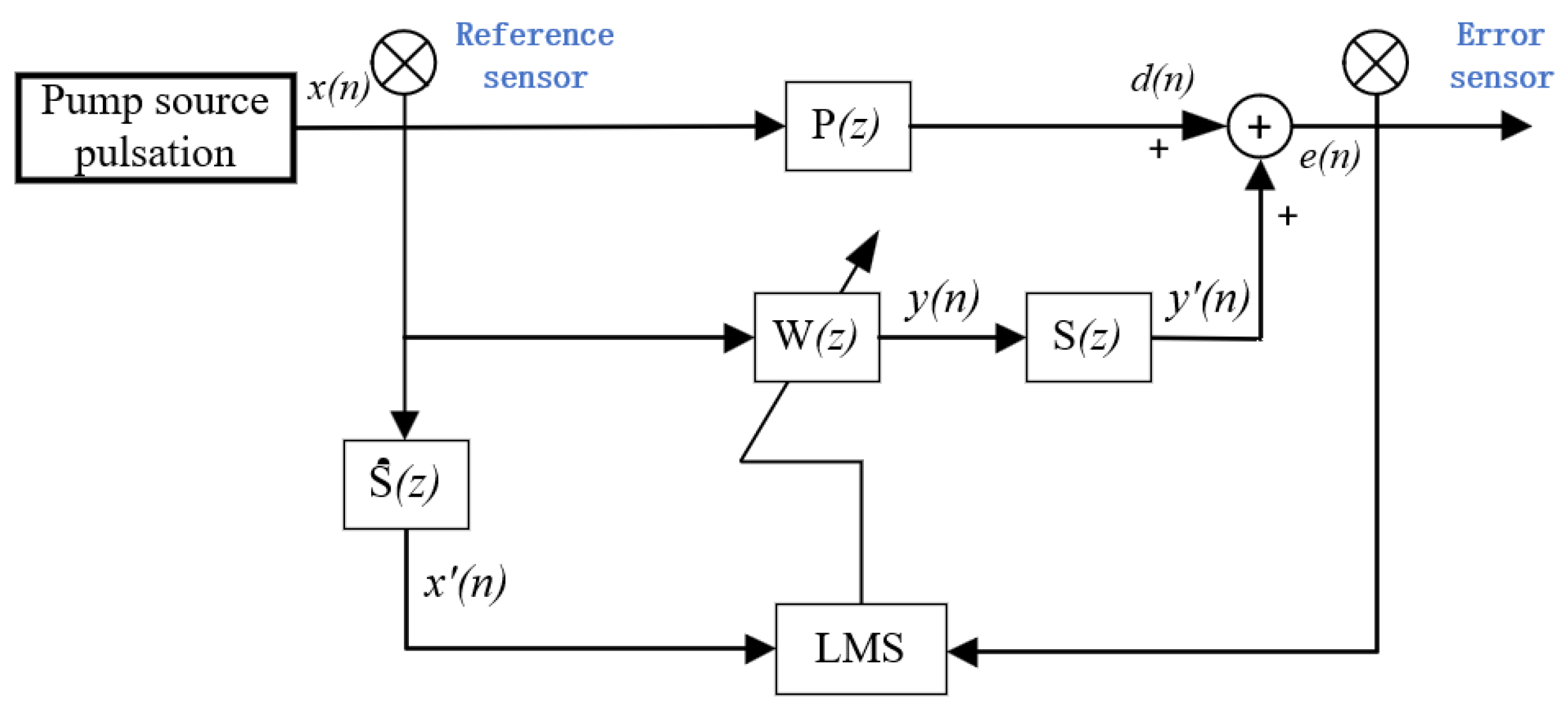
In hydraulic systems, pressure pulsations occur due to the periodic flow pulsations generated by the pump, which propagate through the piping system. These pulsations interact with the piping system’s impedance, resulting in pressure fluctuations. The active control system for hydraulic pulsations employs actuators such as relief valves and servo actuators to generate secondary pulsation waves. These secondary waves interfere with the original pressure pulsation waves in a phase-canceling manner, thereby suppressing the pressure pulsations. However, in active control systems, the actual presence of secondary channels can lead to phase shift and amplitude variations in the filtered output signals $y(n)$, thus affecting the performance of the adaptive algorithm [29]. Conventional LMS cannot be directly applied to such systems, so the FxLMS algorithm, which introduces a secondary channel model, is commonly used for compensating control. The basic principle is shown in Figure 1, where $x(n)$ is the reference signal collected by the reference sensor, $e(n)$ is the error signal measured by the error sensor, $\mathrm{P}(z)$ represents the primary channel, $\mathrm{S}(z)$ is the secondary channel, and ${\mathrm{S}}^{\prime }(z)$ is the estimation of the secondary channel $\mathrm{S}(z)$. In this system, time-domain discrete signals are represented by index n (e.g., $x(n)$), while the transfer functions of the system are represented in the z-transform domain (e.g., $\mathrm{P}(z)$). The same convention is followed in the following text.

In the FxLMS algorithm, the filtered output signal is calculated as:

$$y(n)={\mathit{w}}^T(n)\mathit{x}(n)$$

(1)

where $\mathit{x}(n)={\left[x(n),x(n-1),x(n-2),\dots ,x(n-L+1)\right]}^T$ denotes the input noise vector with length L and $\mathit{w}(n)={\left[w_0(n),w_1(n),w_2(n),\dots ,w_{L-1}(n),\right]}^T$ denotes the weight vector of the controller.

The signal $y^{\prime }(n)$ received by the actuator, i.e., the signal after filtering by the secondary channel, is:

$$y^{\prime }(n)=s(n)\ast y(n)$$

(2)

The residual error obtained by the error sensor is given by the following expression:

$$e(n)=d(n)-y^{\prime }(n)=x(n)\ast p(n)-y(n)\ast s(n)$$

(3)

where $d(n)$ is the desired signal, $p(n)$ and $s(n)$ denote the impulse responses of $\mathrm{P}(z)$ and $\mathrm{S}(z)$, and $\ast$ denotes the linear convolution operator. In the actual control, $s(n)$ is replaced by the estimated pulsation response $\widehat{s}(n)$ of the secondary channel $\widehat{\mathrm{S}}(z)$, so the input signal is filtered by the secondary channel as:

$${\mathit{x}}^{\prime }(n)=\widehat{s}(n)\ast \mathit{x}(n)$$

(4)

According to the most rapid gradient descent method, the FxLMS algorithm updates the filtered weight coefficients with the formula:

$$\mathit{w}(n+1)=\mathit{w}(n)+\mu e(n){\mathit{x}}^{\prime }(n)$$

(5)

where $\mu$ is the step-size (or convergence factor). The process by which the residual error signal $e(n)$ tends toward 0 is the process of gradual convergence of the adaptive algorithm. The steady-state error is the root mean square value of the error signal $e(n)$ after the adaptive filtering process has converged.

Although the fixed step-size FxLMS algorithm is small in computation and simple in structure, it also has obvious drawbacks. Different values of the step-size seriously affect the convergence and stability of the algorithm. A smaller step-size can improve the steady-state accuracy but reduce the convergence rate; a larger step-size speeds up the convergence rate but may lead to larger steady-state error or even algorithm divergence. To overcome the contradictory relationship between convergence rate and steady-state error of the traditional fixed step-size FxLMS algorithm, the variable step-size FxLMS algorithm has emerged.

2.2. Existing Variable Step-Size Strategy

The variable step-size FxLMS algorithm uses the step-size factor $\mu (n)$ to update the step-size in real time, which is a dynamic adjustment method to improve the convergence rate of the adaptive algorithm and reduce the steady-state error. Researchers have carried out in-depth exploration around the step-size adjustment strategy, and proposed a variety of variable step-size algorithms based on nonlinear functions, which optimize the performance of the algorithm by establishing a nonlinear mapping relationship between the step-size and the error. Different nonlinear functions have different shape characteristics and change trends, thus showing their own advantages and disadvantages in convergence performance.

Among them, Zhang et al. [26] proposed a VSS-FxLMS algorithm based on the inverse tangent function, which introduces the inverse tangent function to establish the nonlinear relationship between the error signal $e(n)$ and the step-size $\mu (n)$, and its step-size adjustment formula is:

$$\mu (n)=b\left({\displaystyle \frac{3}{\left(1+\exp {\left(-a\left|\arctan \left(e\left(n\right)\right)\right|\right)}^c\right)}}-1\right)$$

(6)

In the formula, the parameter $a$ is used to regulate the steepness of the step-size function, the value of the parameter $b$ determines the upper limit value of the step, and the parameter $c$ is used to regulate the smoothness of the step-size function at the convergence stage, i.e., in the region of small error, the sensitivity of the step to the error. The algorithm makes full use of the boundedness, continuity, and nonlinear characteristics of the inverse tangent function to achieve a fine dynamic adjustment of the step-size while ensuring the stability of the algorithm. In this case, Equation (5) (weight update formula) is rewritten as:

$$\mathit{w}(n+1)=\mathit{w}(n)+\mu (n)e(n){\mathit{x}}^{\prime }(n)$$

(7)

In contrast to the traditional FxLMS algorithm with a fixed step-size $\mu$, the step-size of the weight update of this algorithm is time-varying, and the magnitude of the weight update is adaptively changed according to the magnitude of the error.

In addition to the above algorithms based on the inverse tangent function, researchers have designed various variable step-size strategies based on different mathematical models.

Table 1. Representative variable step-size strategies.

Algorithm Name/Proposer	Step-Size Function Formula
VSSLMS-1/Wang [30]	$\mu (n)=b\left({\displaystyle \frac{1}{1+\exp \left(-aE\left[e\left(n-1\right)e\left(n\right)\right]\right)}}-0.5\right)$
VSSLMS-2/Qian	$\mu (n)=\beta \left({\displaystyle \frac{{\left|e\left(n\right)\right|}^m}{\alpha {\left|e\left(n\right)\right|}^m+1}}\right)$
VSSLMS-3/Zhang	$\mu (n)=b\left({\displaystyle \frac{3}{\left(1+\exp {\left(-a\left|\arctan \left(e\left(n\right)\right)\right|\right)}^c\right)}}-1\right)$

summarises several representative variable step-size strategies.

These algorithms establish step-size and error functional relationships through distinct mathematical models. While these functions exhibit distinct characteristics, they share common limitations: The exponential step-size function demonstrates rapid convergence in large-error regions, but exhibits inadequate precision control in small-error regions, frequently resulting in substantial steady-state errors or oscillations. Power function-based step-size algorithms achieve improved steady-state performance at the expense of delayed response to abrupt errors, consequently degrading tracking capability. Arctangent function-based approaches attempt to balance these criteria, yet demonstrate limited adaptability in non-stationary environments, particularly during abrupt noise variations where performance remains suboptimal. Current variable step-size adaptive algorithms struggle to simultaneously satisfy convergence rate, tracking capability, and steady-state error requirements in practical implementations.

3. Proposed DNVSS-FxLMS Algorithm

In order to obtain fast convergence rate as well as superior steady-state error, this paper proposes a variable step-size FxLMS algorithm based on the combination of dual nonlinearities, whose corresponding step-size equation is:

$$\mu (n)={\mu }_{\max }\cdot {\displaystyle \frac{e^2(n)}{e^2(n)+{\beta }^2}}\cdot \left(1-e^{-\alpha \left|e(n)\right|}\right)$$

(8)

Among them, ${\mu }_{\max }$, $\alpha$, and $\beta$ are the three defined parameters; by adjusting the values of these parameters, the shape characteristics of the step-size function curve can be precisely controlled. The effects of the three parameters on the step curve are shown in Figure 2 (assuming that the error $e(n)$ is in the size range of [−2,2]).

The mechanism of each parameter can be clearly observed from Figure 2: the parameter ${\mu }_{\max }$ is used to control the upper bound value of the step-size, and also influences the value of the step-size in the large error region, which will directly determine the initial convergence rate of the algorithm. The parameter $\alpha$ is used to control the sensitivity of the step-size function to small errors, i.e., to regulate the rate of change of the step-size, so the value of $\alpha$ will be closely related to the steady-state error of the algorithm. When $\alpha$ is larger, the step-size is more sensitive to small errors, which increases the steady-state error; when $\alpha$ is smaller, the step-size is not sensitive to small errors, which is conducive to obtaining a smaller steady-state error. The parameter $\beta$ is used to regulate the transition stage of large and small step-size. The smaller the value of $\beta$, the wider the range of large step-size, which is conducive to the rapid convergence of the algorithm, but at the same time, it will compress the interval of the small step-size, which will seriously affect the steady-state error; the larger the value of $\beta$, the algorithm will enter into the stage of small step-size of, which is conducive to the stability of the algorithm, but it will reduce the initial convergence rate of the system.

The step-size function cleverly combines the two nonlinear mechanisms of rational fractional term and exponential term to achieve the adaptive adjustment of the step-size. Monotonicity: the derivation of the step-size function is ${\displaystyle \frac{d\mu \left(n\right)}{d\left|e\left(n\right)\right|}}>0$, which verifies the monotonicity of the step-size function with respect to the absolute value of the error. This property ensures the ideal adjustment mechanism of “the larger the error, the larger the step-size to accelerate convergence; the smaller the error, the smaller the step-size to improve accuracy”. Boundedness: when $\left|e\left(n\right)\right|\to 0$, $\mu \left(n\right)\to 0$; when $\left|e\left(n\right)\right|\to \infty$, $\mu \left(n\right)\to {\mu }_{\max }$. Combined with the monotonicity of the step-size function, $0\le \mu \left(n\right)\le {\mu }_{\max }$, this ensures that the algorithm will not exceed the range of stable convergence under any circumstances.

From the perspective of function design, the rational fraction term provides smooth step-size transition during the error change process, effectively avoiding the sudden change of the step-size, and thus enhancing the stability of the algorithm; the exponential term changes smoothly in the small error range, and is able to provide delicate step-size control. Through the proper configuration of the parameters, the organic combination of the rational fraction and exponential functions enables the step-size function to maintain a large step-size in the early convergence stage accelerating the convergence rate, while maintaining a small step-size in the small error range, thus ensuring a low mean squared error.

The symmetrical design of this algorithm runs through three levels: Firstly, at the physical level, the active control of hydraulic pulsation is based on the principle of phase symmetrical cancellation, and the symmetrical cancellation of the pressure wave is achieved by generating a secondary signal with a phase difference of $\pi$ from the original pulsation. Secondly, at the mathematical level, the proposed step-size function $\mu \left(e\left(n\right)\right)$ has an even symmetry property with respect to $e\left(n\right)=0$. This symmetry ensures that the algorithm has the same adjustment ability for positive and negative errors and enhances the stability of the system. Finally, at the performance level, through the symmetrical coupling mechanism of rational fraction terms and exponential terms, the algorithm achieves a symmetrical balance between convergence speed and steady-state accuracy. Fast convergence does not come at the expense of steady-state accuracy, and low steady-state errors do not affect the initial convergence speed. This multi-level symmetrical design not only endows the algorithm with an elegant mathematical structure, but also ensures its robustness and excellent control performance in complex time-varying environments.

4. Algorithm Performance Analysis

4.1. Complexity Analysis

The computational complexity is a key indicator to assess whether the algorithm is suitable for real-time control systems, which directly affects the practical engineering realizability of the algorithm.

Table 2. Complexity of different FxLMS algorithms in a single iteration process.

Algorithm	Number of Multiplications/Divisions	Number of Additions/Subtractions	Special Functions
FxLMS	2L + 2M + 1	2L + 2M − 2	0
VSSFxLMS-1/ Wang	2L + 2M + 5	2L + 2M	1
VSSFxLMS-2/ Qian	2L + 2M + 4	2L + 2M − 1	1
VSSFxLMS-3/ Zhang	2L + 2M + 7	2L + 2M	3
DNVSS-FxLMS	2L + 2M + 7	2L + 2M	2

compares and analyzes the computational complexity of the DNVSS-FxLMS algorithm with several existing variable step-size algorithms during a single iteration, demonstrating the computational efficiency of the proposed algorithm.

In the Table 2, L denotes the length of the adaptive filter and M denotes the length of the secondary path. Special functions include exponential, absolute value, logarithmic, and inverse trigonometric functions.

As can be seen from Table 2, the computational complexity of the proposed DNVSS-FxLMS algorithm is slightly higher than that of the FxLMS and VSSFxLMS-1 and -2 algorithms, and more arithmetic operations need to be performed; however, these additional computational overheads are independent of the length of the filter and the length of the secondary path. Therefore, this increase in relative computational cost becomes negligible for medium or large filter scenarios that are common in real-world applications. It is worth noting that compared to the VSSFxLMS-3 algorithm, which has better performance, both algorithms have comparable computational complexity, but DNVSS-FxLMS requires fewer special function calls, which is an advantage in practical applications. In summary, the proposed DNVSS-FxLMS algorithm achieves the dual optimization goals of improving the convergence rate and reducing the steady-state error while ensuring that the computational complexity is within an acceptable range, demonstrating a good balance of algorithmic efficiency and engineering practicality.

4.2. Convergence Analysis

For a rigorous mathematical analysis, the following assumptions are first introduced:

• The input signal $\mathit{x}(n)$ is a generalised smooth stochastic process with zero mean and variance ${{\sigma }_x}^2$;
• The noise $\xi (n)$ is white noise with zero mean and variance ${{\sigma }_x}^2$ and is uncorrelated with the input signal $\mathit{x}(n)$;
• The desired signal $d(n)$ satisfies the linear model: $d(n)={{\mathit{w}}_{opt}}^T\mathit{x}(n)+\xi (n)$, ${\mathit{w}}_{opt}$ are the optimal weight vectors;
• The initial weights $\mathit{w}(0)$ are uncorrelated with the input signal and noise;
• Independence assumptions: $\mathit{v}(n)$, $\xi (n)$, and $\mathit{x}(n)$ are approximately independent.

4.2.1. Mean Convergence Analysis

The update equation for the DNVSS-FxLMS algorithm is:

$$\mathit{w}(n+1)=\mathit{w}(n)+\mu (n)e(n){\mathit{x}}^{\prime }(n)$$

(9)

Defining the weight error vector $\mathit{v}(n)=\mathit{w}(n)-{\mathit{w}}_{opt}$, there is:

$$\mathit{v}(n+1)=\mathit{v}(n)+\mu (n)e(n){\mathit{x}}^{\prime }(n)$$

(10)

The error signal $e(n)$ can be expressed as:

$$e(n)=d(n)-s\left(n\right)\ast \left[{\mathit{w}}^T(n)\mathit{x}(n)\right]=\xi (n)-{\mathit{v}}^T(n){\mathit{x}}^{\prime }(n)$$

(11)

Substitute the error expression into the weighting error update equation:

$$\mathit{v}(n+1)=\mathit{v}(n)+\mu (n)\left[\xi \left(n\right)-{\mathit{v}}^T(n){\mathit{x}}^{\prime }(n)\right]{\mathit{x}}^{\prime }(n)$$

(12)

Take expectations for both sides of the above equation:

$$E\left[\mathit{v}\left(n+1\right)\right]=E\left[\mathit{v}\left(n\right)\right]+E\left[\mu \left(n\right)\xi \left(n\right){\mathit{x}}^{\prime }\left(n\right)\right]-E\left[\mu \left(n\right){\mathit{x}}^{\prime }\left(n\right){{\mathit{x}}^{\prime }}^T\left(n\right)\mathit{v}\left(n\right)\right]$$

(13)

Since the assumptions $\mathit{v}(n)$, $\xi (n)$ are independent of $\mathit{x}(n)$ and $E[\xi (n)]=0$, therefore:

$$E\left[\mu \left(n\right)\xi \left(n\right){\mathit{x}}^{\prime }\left(n\right)\right]=0$$

(14)

It can be obtained under the assumption of independence:

$$E\left[\mathit{v}\left(n+1\right)\right]=E\left[\mathit{v}\left(n\right)\right]-E\left[\mu \left(n\right)\right]E\left[{\mathit{x}}^{\prime }\left(n\right){{\mathit{x}}^{\prime }}^T\left(n\right)\right]E\left[\mathit{v}\left(n\right)\right]$$

(15)

Let $\mathbf{R}=E\left[{\mathit{x}}^{\prime }(n){{\mathit{x}}^{\prime }}^T(n)\right]$ be the autocorrelation matrix of ${\mathit{x}}^{\prime }(n)$ and $\mathbf{I}$ be the unit matrix of $L\times L$. Therefore, the mean update equation simplifies to:

$$E\left[\mathit{v}\left(n+1\right)\right]=\left[\mathbf{I}-E\left[\mu \left(n\right)\right]\mathbf{R}\right]E\left[\mathit{v}\left(n\right)\right]$$

(16)

The recursive solution is obtained:

$$E\left[\mathit{v}\left(n\right)\right]={\displaystyle \prod _{i=0}^{n-1}\left[\mathbf{I}-E\left[\mu \left(i\right)\right]\mathbf{R}\right]E\left[\mathit{v}\left(0\right)\right]}$$

(17)

To ensure that $li{m}_{n\to \infty }E\left[\mathit{v}\left(n\right)\right]=0$, the algorithm mean converges, it is necessary to ensure that the sequence of matrices ${\displaystyle \prod \begin{array}{l}n-1\\ i=0\end{array}}\left[\mathbf{I}-E\left[\mu \left(i\right)\right]\mathbf{R}\right]$ converges to the zero matrix.

Assume that $\mathbf{R}$ is diagonalisable, i.e., $\mathbf{R}=\mathbf{Q}\mathbf{\Lambda }{\mathbf{Q}}^{-1}$, where $\Lambda =\mathrm{diag}({\lambda }_1,{\lambda }_2,\dots ,{\lambda }_N)$ contains the eigenvalues of $\mathbf{R}$ and $\mathbf{Q}$’s is the corresponding eigenvector matrix. Then:

$$\begin{array}{l}{\displaystyle \prod _{i=0}^{n-1}\left[\mathbf{I}-E\left[\mu \left(i\right)\right]\mathbf{R}\right]}=\mathbf{Q}\left[{\displaystyle \prod _{i=0}^{n-1}\left[\mathbf{I}-E\left[\mu \left(i\right)\right]\Lambda \right]}\right]{\mathbf{Q}}^{-1}\\ =\mathbf{Q}diag\left({\displaystyle \prod _{i=0}^{n-1}\left[1-E\left[\mu \left(i\right)\right]{\lambda }_1\right]},{\displaystyle \prod _{i=0}^{n-1}\left[1-E\left[\mu \left(i\right)\right]{\lambda }_2\right]},\dots ,{\displaystyle \prod _{i=0}^{n-1}\left[1-E\left[\mu \left(i\right)\right]{\lambda }_N\right]}\right){\mathbf{Q}}^{-1}\end{array}$$

(18)

For each eigenvalue ${\lambda }_j$, to make $\underset{n\to \infty }{\lim }{\displaystyle \prod \begin{array}{l}n-1\\ i=0\end{array}}\left[1-E\left[\mu \left(i\right)\right]{\lambda }_j\right]=0$, it needs to be satisfied:

$$\left|1-E\left[\mu \left(i\right)\right]{\lambda }_j\right|<1$$

(19)

To wit:

$$0<E\left[\mu \left(i\right)\right]<{\displaystyle \frac{2}{{\lambda }_j}}$$

(20)

In particular, to ensure that the above condition holds for all eigenvalues, it needs to be satisfied:

$$0<E\left[\mu \left(n\right)\right]<{\displaystyle \frac{2}{{\lambda }_{max}}}$$

(21)

where ${\lambda }_{max}$ is the largest eigenvalue of $\mathbf{R}$.

Since the DNVSS-FXLMS algorithm in $\mu \left(n\right)\le {\mu }_{max}$, and $E\left[\mu \left(n\right)\right]\le {\mu }_{max}$, this leads to the following important results:

Theorem 1

(Mean convergence condition). The sufficient condition for mean convergence of the DNVSS-FxLMS algorithm is:

$$0<{\mu }_{max}<{\displaystyle \frac{2}{{\lambda }_{max}}}$$

(22)

This result indicates that, despite the use of a variable step-size mechanism based on a double nonlinear function, the DNVSS-FxLMS algorithm maintains the same mean convergence conditions as the standard LMS algorithm, which is of great significance for practical applications.

4.2.2. Mean Square Convergence Analysis

The mean square convergence analysis examines the convergence of the covariance matrix of the weight errors $\mathbf{K}(n)=E[v(n)v^T(n)]$. From the weight error update equation:

$$\mathit{v}(n+1)=\mathit{v}(n)+\mu (n)\left[\xi \left(n\right)-{\mathit{v}}^T(n){\mathit{x}}^{\prime }(n)\right]{\mathit{x}}^{\prime }(n)$$

(23)

The two side tensor products and taking the expectation, expanded and collapsed, are obtained after a complex mathematical derivation [31], using Assumptions 3 and 5:

$$\mathbf{K}\left(n+1\right)=\left(\mathbf{I}-E\left[\mu \left(n\right)\right]\mathbf{R}\right)\mathbf{K}\left(n\right)\left(\mathbf{I}-E\left[\mu \left(n\right)\right]\mathbf{R}\right)+E\left[{\mu }^2\left(n\right)\right]{{\sigma }_v}^2\mathbf{R}+O({\mu }^3)$$

(24)

where $O(E[{\mu }^2(n)])$ denotes the higher-order minors.

To ensure that $\mathbf{K}(n)$ converges to a finite value, certain conditions need to be satisfied. According to Bismor et al. [8], the sufficient condition for mean square convergence is:

$$0<{\displaystyle \frac{E\left[{\mu }^2\left(n\right)\right]}{E\left[\mu \left(n\right)\right]}}<{\displaystyle \frac{2}{3\cdot tr(\mathit{R})}}$$

(25)

where $tr(~)$ denotes the trace of the matrix; for the DNVSS-FXLMS algorithm, the above condition is easier to satisfy in the later stages of convergence because the step-size $\mu (n)$ decreases during the convergence process, which makes ${\displaystyle \frac{E[{\mu }^2(n)]}{E[\mu (n)]}}$ decrease as well. In addition, due to the symmetrical design of the step-size function, the algorithm has symmetrical response characteristics to positive and negative error disturbances, which ensures the stable convergence of the system under bidirectional disturbances.

4.3. Steady-State Analysis

4.3.1. Steady-State Mean Square Error Analysis

According to adaptive filtering theory, the mean square error can be decomposed as:

$$E\left[e^2(n)\right]={\xi }_{min}+{\xi }_{ex}(n)$$

(26)

where ${\xi }_{min}=E\left[{\xi }^2\left(n\right)\right]={{\sigma }_{\xi }}^2$ is the minimum mean square error and ${\xi }_{ex}(n)=E\left[{\mathbf{V}}^T(n)\mathbf{R}\mathbf{V}(n)\right]$ is the excess mean square error (EMSE). Using the weights error covariance matrix defined earlier $\mathbf{K}(n)=E\left[\mathbf{V}(n){\mathbf{V}}^T(n)\right]$ then:

$${\xi }_{ex}(n)=\mathrm{tr}\left[\mathbf{R}\mathbf{K}(n)\right]$$

(27)

In order to analyze the steady-state performance, we need to make use of the recursive relationship of $\mathbf{K}(n)$ obtained in Equation (24):

$$\mathbf{K}\left(n+1\right)=\left(\mathbf{I}-E\left[\mu \left(n\right)\right]\mathbf{R}\right)\mathbf{K}\left(n\right)\left(\mathbf{I}-E\left[\mu \left(n\right)\right]\mathbf{R}\right)+E\left[{\mu }^2\left(n\right)\right]{{\sigma }_v}^2\mathbf{R}+O({\mu }^3)$$

(28)

Define $\tilde{\mathbf{K}}(n)={\mathbf{Q}}^T\mathbf{K}\left(n\right)\mathbf{Q}$ then:

$$\tilde{\mathbf{K}}\left(n+1\right)=\left(\mathbf{I}-E\left[\mu \left(n\right)\right]\Lambda \right)\tilde{\mathbf{K}}\left(n\right)\left(\mathbf{I}-E\left[\mu \left(n\right)\right]\Lambda \right)+E\left[{\mu }^2\left(n\right)\right]{{\sigma }_v}^2\Lambda +O({\mu }^3)$$

(29)

In steady-state, $\tilde{\mathbf{K}}\left(n+1\right)=\tilde{\mathbf{K}}\left(n\right)=\tilde{\mathbf{K}}\left(\infty \right)$. So, for diagonal elements ${\tilde{k}}_{ii}\left(\infty \right)$:

$${\tilde{k}}_{ii}\left(\infty \right)={\left(1-E\left[\mu \left(\infty \right)\right]{\lambda }_i\right)}^2{\tilde{k}}_{ii}\left(\infty \right)+E\left[{\mu }^2\left(\infty \right)\right]{{\sigma }_v}^2{\lambda }_i+O({\mu }^3)$$

(30)

Solution:

$${\tilde{k}}_{ii}\left(\infty \right)\approx {\displaystyle \frac{{\lambda }_i{{\sigma }_{\xi }}^{2}E\left[{\mu }^2\left(\infty \right)\right]}{2{\lambda }_{i}E\left[\mu \left(\infty \right)\right]-{{\lambda }_i}^{2}E\left[{\mu }^2\left(\infty \right)\right]}}$$

(31)

The resulting steady-state EMSE is:

$$\begin{gathered} {\xi }_{ex}\left(\infty \right)=\mathrm{tr}\left[\mathbf{R}\mathbf{K}\left(\infty \right)\right]=\mathrm{tr}\left[\Lambda \tilde{\mathbf{K}}\left(\infty \right)\right]={\displaystyle \sum _{i=1}^L{\lambda }_i{\tilde{k}}_{ii}\left(\infty \right)} \\ ={\displaystyle \sum _{i=1}^L\frac{{{\lambda }_i}^2{{\sigma }_{\xi }}^{2}E\left[{\mu }^2\left(\infty \right)\right]}{2{\lambda }_{i}E\left[\mu \left(\infty \right)\right]-{{\lambda }_i}^{2}E\left[{\mu }^2\left(\infty \right)\right]}} \end{gathered}$$

(32)

When ${\lambda }_{i}E\left[\mu \left(\infty \right)\right]\ll 1$ is used, the above equation can be approximated:

$${\xi }_{ex}\left(\infty \right)\approx {\displaystyle \frac{1}{2}}{\displaystyle \sum _{i=1}^L{\lambda }_i{{\sigma }_{\xi }}^2\frac{E\left[{\mu }^2\left(\infty \right)\right]}{E\left[\mu \left(\infty \right)\right]}}={\displaystyle \frac{E\left[{\mu }^2\left(\infty \right)\right]}{2E\left[\mu \left(\infty \right)\right]}}{{\sigma }_{\xi }}^2\mathrm{tr}\left(\mathbf{R}\right)$$

(33)

4.3.2. Mismatch Analysis

Mismatch $M$ is defined as the ratio of EMSE to the minimum MSE:

$$M={\displaystyle \frac{{\xi }_{ex}\left(\infty \right)}{{\xi }_{\min }}}={\displaystyle \frac{{\xi }_{ex}\left(\infty \right)}{{{\sigma }_{\xi }}^2}}$$

(34)

Combined with Equation (33), this yields

$$M={\displaystyle \frac{E\left[{\mu }^2\left(\infty \right)\right]}{2E\left[\mu \left(\infty \right)\right]}}\mathrm{tr}\left(\mathbf{R}\right)$$

(35)

For the variable step-size function proposed in this paper, when the error $e\left(n\right)$ is very small, the step-size function $\mu \left(n\right)$ can be approximated by Taylor expansion:

$$\mu \left(n\right)\approx {\mu }_{max}\cdot {\displaystyle \frac{\alpha {\left|e\left(n\right)\right|}^3}{{\beta }^2}}$$

(36)

This suggests that as the algorithm approaches convergence, the step-size is proportional to the third power of the error mean, which allows the step-size to be more sensitive to changes in the error.

Based on this approximation, the expected value of the step-size at steady-state can be expressed as:

$$E\left[\mu \left(\infty \right)\right]\approx {\mu }_{\max }\cdot {\displaystyle \frac{\alpha }{{\beta }^2}}\cdot E\left[{\left|e\left(\infty \right)\right|}^3\right]$$

(37)

Since the filtered weights are close to the optimal weights at steady-state $w_{opt}$, then $v\left(n\right)\to 0$, so:

$$e\left(n\right)\approx \xi \left(n\right)$$

(38)

This shows that at steady-state, $e\left(n\right)$ also approximately obeys a Gaussian distribution with mean 0 and variance ${{\sigma }_{\xi }}^2$. For a zero-mean Gaussian random variable $e\left(n\right)$, there is $E\left[{\left|e\left(\infty \right)\right|}^3\right]={\displaystyle \frac{2\sqrt{2}}{\sqrt{\pi }}}{{\sigma }_{\xi }}^3$, so:

$$E\left[\mu \left(\infty \right)\right]\approx {\mu }_{\max }\cdot {\displaystyle \frac{\alpha }{{\beta }^2}}\cdot {\displaystyle \frac{2\sqrt{2}}{\sqrt{\pi }}}\cdot {{\sigma }_{\xi }}^3$$

(39)

Similarly, the second order moments of the step-size function are:

$$E\left[{\mu }^2\left(\infty \right)\right]\approx {{\mu }^2}_{\max }\cdot {\displaystyle \frac{{\alpha }^2}{{\beta }^4}}\cdot E\left[{\left|e\left(\infty \right)\right|}^6\right]$$

(40)

For a zero-mean Gaussian random variable $e\left(n\right)$, there is $E\left[{\left|e\left(\infty \right)\right|}^6\right]=15{{\sigma }_e}^6$, so:

$$E\left[{\mu }^2\left(\infty \right)\right]\approx {{\mu }^2}_{\max }\cdot {\displaystyle \frac{{\alpha }^2}{{\beta }^4}}\cdot 15\cdot {{\sigma }_{\xi }}^6$$

(41)

Define the ratio $\gamma ={\displaystyle \frac{E\left[{\mu }^2\left(\infty \right)\right]}{E\left[\mu \left(\infty \right)\right]}}$, obtained from the above results:

$$\gamma \approx {\mu }_{\max }\cdot {\displaystyle \frac{\alpha }{{\beta }^2}}\cdot {\displaystyle \frac{15\sqrt{\pi }}{2\sqrt{2}}}\cdot {{\sigma }_{\xi }}^3$$

(42)

Substituting this equation into Equation (35) and simplifying, we obtain an important theoretical result of the algorithm:

Theorem 2

(Steady-state mismatch property). For the DNVSS-FxLMS algorithm, steady-state mismatch satisfies:

$$M={\displaystyle \frac{15\sqrt{\pi }}{4\sqrt{2}}}\cdot {\mu }_{\max }\cdot {\displaystyle \frac{\alpha }{{\beta }^2}}\cdot {{\sigma }_{\xi }}^3\cdot \mathrm{tr}\left(\mathbf{R}\right)$$

(43)

This equation shows that the mismatch is proportional to the third power of the noise variance, instead of the linear relationship of the traditional FxLMS algorithm. In a high SNR environment (${{\sigma }_{\xi }}^2$ is smaller), the mismatch decreases at a cubic rate, achieving very low steady-state error; in a low SNR environment (${{\sigma }_{\xi }}^2$ is larger), the steady-state mismatch of the algorithm can be further reduced by adjusting the parameter of the step-size function, achieving low steady-state error.

Combining the above performance analyses, the DNVSS-FxLMS algorithm proposed in this paper achieves adaptive adjustment of the step-size to the error magnitude by coupling the two nonlinear mechanisms of rational fraction and exponential terms, which ensures fast convergence while obtaining a low steady-state EMSE.

5. Simulation System Experiment

Active control of hydraulic system pressure pulsations faces three major technical challenges: (1) rapid convergence is required to respond to system startup and operating condition changes; (2) high-precision steady-state control is required to meet equipment accuracy requirements; and (3) excellent time-varying tracking capability is required to adapt to system parameter changes. Therefore, in this section, the comprehensive performance of the proposed DNVSS-FxLMS algorithm under time-varying system conditions is evaluated through simulation analysis. To fully verify the effectiveness and performance advantages of the algorithm, it is analyzed and compared to four algorithms: the traditional fixed step-size FxLMS algorithm and three variable step-size algorithms (VSSFxLMS-1/Wang, VSSFxLMS-2/Qian, and VSS-FxLMS-3/Zhang). The simulation experiments focus on the performance of the algorithms in terms of three key performance indicators: convergence rate, steady-state error, and time-varying tracking performance.

In terms of the simulation system configuration, a 64-order FIR adaptive filter structure (M = 64) is used, and the reference signal $x(n)$ is filtered with a 32-order low-pass FIR filter using Gaussian white noise, then normalized to obtain a colored signal with frequency correlation. The filtering process simulates the non-uniform distribution of the spectrum caused by the pipeline transmission characteristics and pump pulsation characteristics in the actual working conditions of the hydraulic system. This processing leads to a significant eigenvalue dispersion in the input autocorrelation matrix, truly reflecting the spectral characteristics of pressure pulsation in the hydraulic system and the complex noise environment in practical applications. This stiffness characteristic requires the control algorithm to be able to handle both fast and slow converging modes simultaneously, which is precisely the advantage of the variable step-size algorithm. In the simulation process, the signal-to-noise ratio of the colored noise environment is set to 25 dB.

For the secondary path model used in the FxLMS algorithm, a 16th-order FIR low-pass filter is employed. To simplify the simulation analysis, it is assumed that the secondary paths are perfectly identified (i.e., the effect of secondary path modeling errors is ignored). All simulations are performed for 10,000 iterations, with results averaged over 200 independent Monte Carlo simulation experiments to ensure statistical reliability. The key parameters of each algorithm are set in

Table 3. Parameter values for different FxLMS algorithms.

Algorithm	Parameter Value
FxLMS	$\mu =0.0002$
VSSFxLMS-1/ Wang	$a=3$, $b=0.00437$
VSSFxLMS-2/ Qian	$\alpha =5$, $\beta =0.01094$, $m=3$
VSSFxLMS-3/ Zhang	$a=5$, $b=0.00078$, $c=4$
DNVSS-FxLMS	${\mu }_{\max }=0.00219$, $\alpha =8.5$, $\beta =0.12$

.

The performance characteristics of the algorithms will be analyzed and discussed through four typical case studies simulating different hydraulic system working environments.

5.1. Case 1: System Mutation

In this case, the ability of the algorithms to track the response of a time-varying system is analyzed by introducing a sudden step change in the system parameters. This setup is designed to simulate a scenario in which the pressure pulsation characteristics of a hydraulic system change due to switching of operating conditions or a sudden change in load.

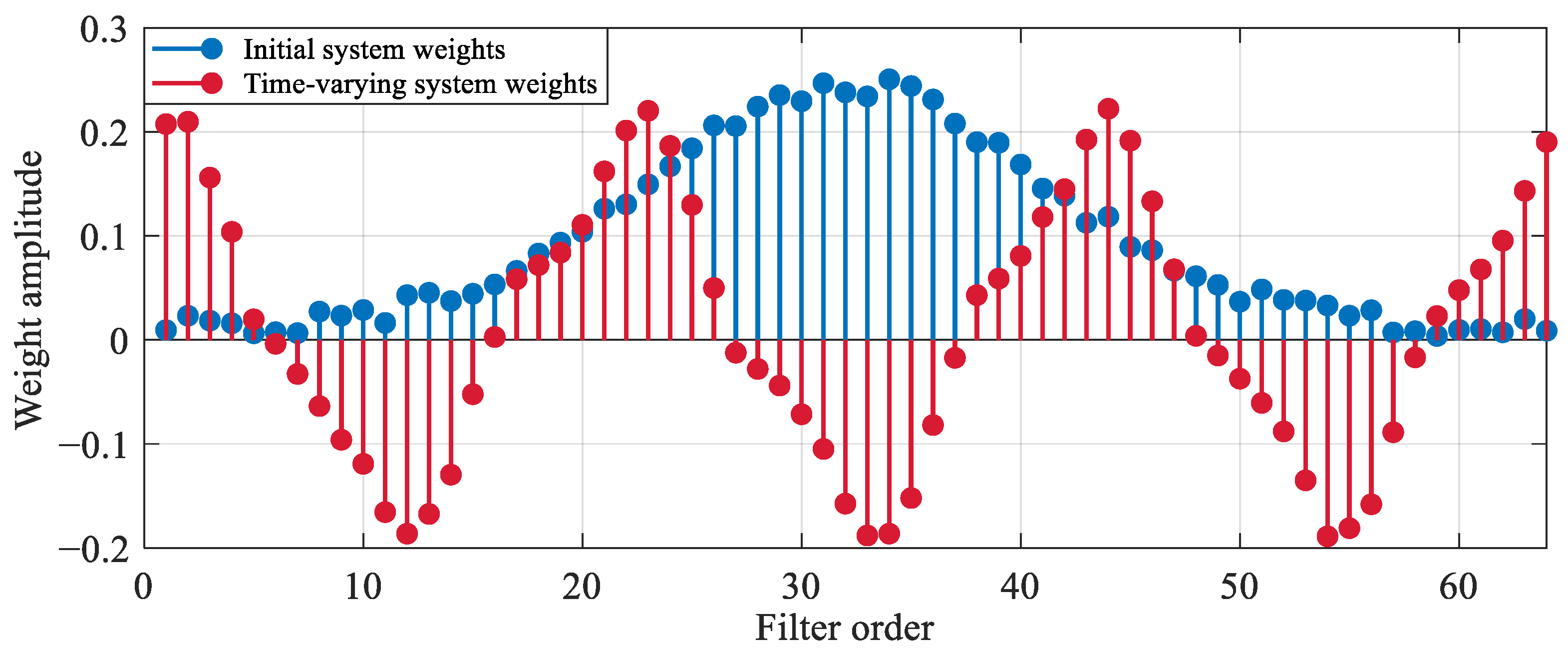
The configuration of the simulation experiment is as follows: a sudden change in the system parameters is introduced at the 5000th iteration. The system is set with different weight coefficients before and after the time-varying, forming two stages with distinct characteristics. The specific distribution of the system weights before and after the time-variation is shown in Figure 3.

The initial system uses a bell-shaped weight distribution with the largest central amplitude and a mathematical expression:

$$w_{init}\left(i\right)=\exp \left(-{\left({\displaystyle \frac{i-M/2}{M/5}}\right)}^2\right)+0.1\cdot rand$$

(44)

The time-varying posterior system (after the 5000th iteration) uses an oscillating weight distribution with the following structure:

$$w_{change}\left(i\right)=\cos \left({\displaystyle \frac{6\pi i}{M}}\right)\left(0.7+0.3\sin \left({\displaystyle \frac{12\pi i}{M}}\right)\right)+0.1\cdot rand$$

(45)

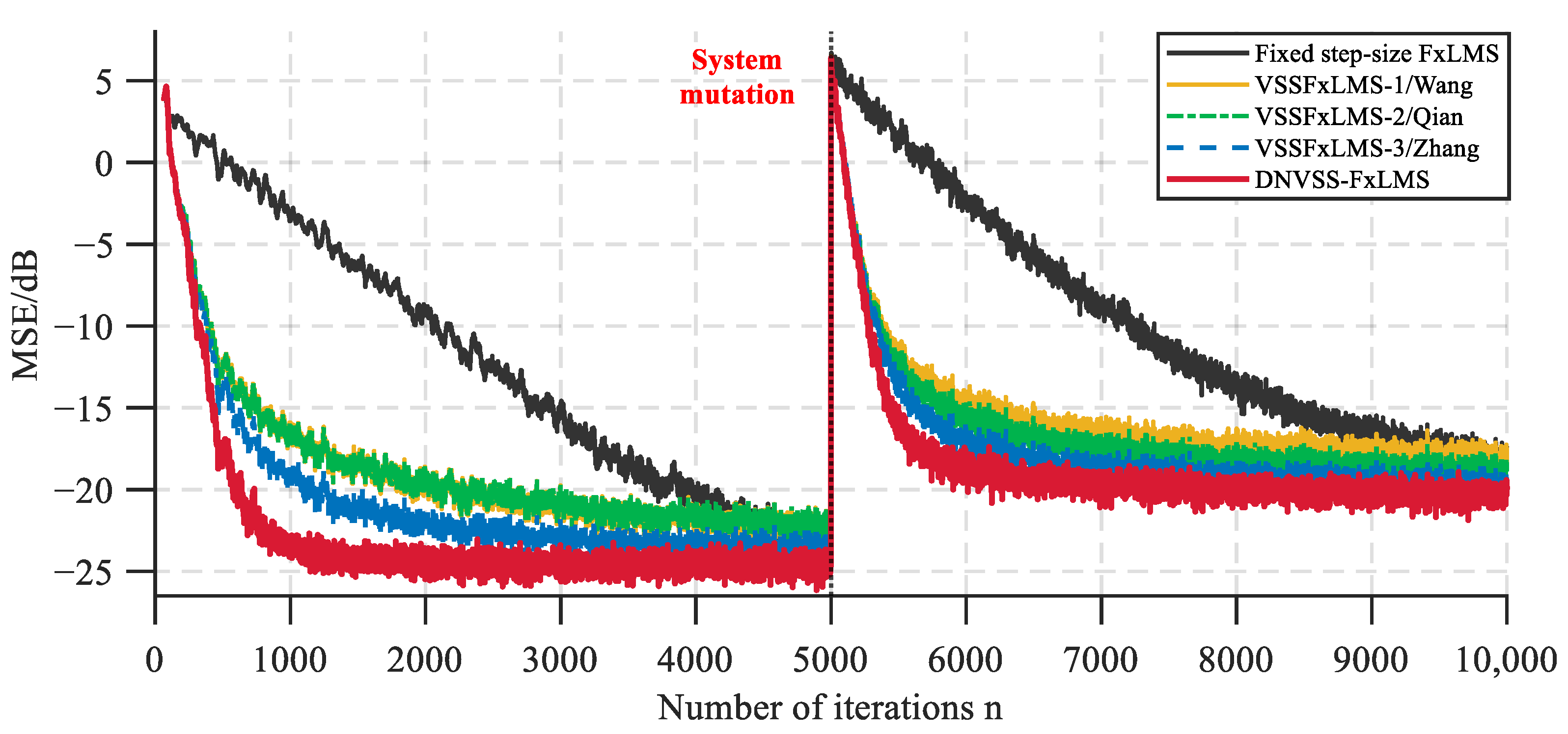
The results of the simulation experiments in this environment are shown in Figure 4.

From the MSE change curve in Figure 4, it can be seen that the convergence rate of the DNVSS-FxLMS algorithm in the initial stage is significantly faster than that of the other variable step-size algorithms. When the system undergoes a sudden change at 5000 iterations, the algorithm can still converge to the new steady-state quickly, demonstrating good tracking performance. Additionally, the proposed algorithm achieves the lowest steady-state error. In the initial stage, the steady-state MSE remains around −24.7 dB. After the system undergoes a sudden change, the steady-state MSE remains around −20.3 dB. Compared with other algorithms, it improves by at least 1–3 dB, demonstrating superior steady-state performance. This fast convergence and low steady-state error characteristics make the algorithm particularly suitable for hydraulic equipment that frequently switches operating conditions. The specific performance comparison of various algorithms is shown in

Table 4. Performance comparison of different algorithms when the system undergoes mutation.

Algorithm	Initial Stage (n = 0)			System Mutation (n = 5000)
	Convergence Point	Convergence Speed	MSE (dB)	Convergence Point	Convergence Speed	MSE (dB)
FxLMS	4172	4172	−23.0	9223	4223	−17.3
VSSFxLMS-1/ Wang	2605	2605	−22.1	7557	2557	−17.6
VSSFxLMS-2/ Qian	2600	2600	−22.1	6894	1894	−18.4
VSSFxLMS-3/ Zhang	2206	2206	−23.3	6293	1293	−19.3
DNVSS-FxLMS	1167	1167	−24.7	5894	894	−20.3

.

In the table, the convergence point indicates the point at which the algorithm reaches a steady state from the initial state or after a system mutation; the convergence speed refers to the number of iterations required to reach the steady state; MSE (dB): the mean square error expressed in decibels, used to evaluate the algorithm’s pulsation suppression capability.

5.2. Case 2: Different Signal-to-Noise Ratios

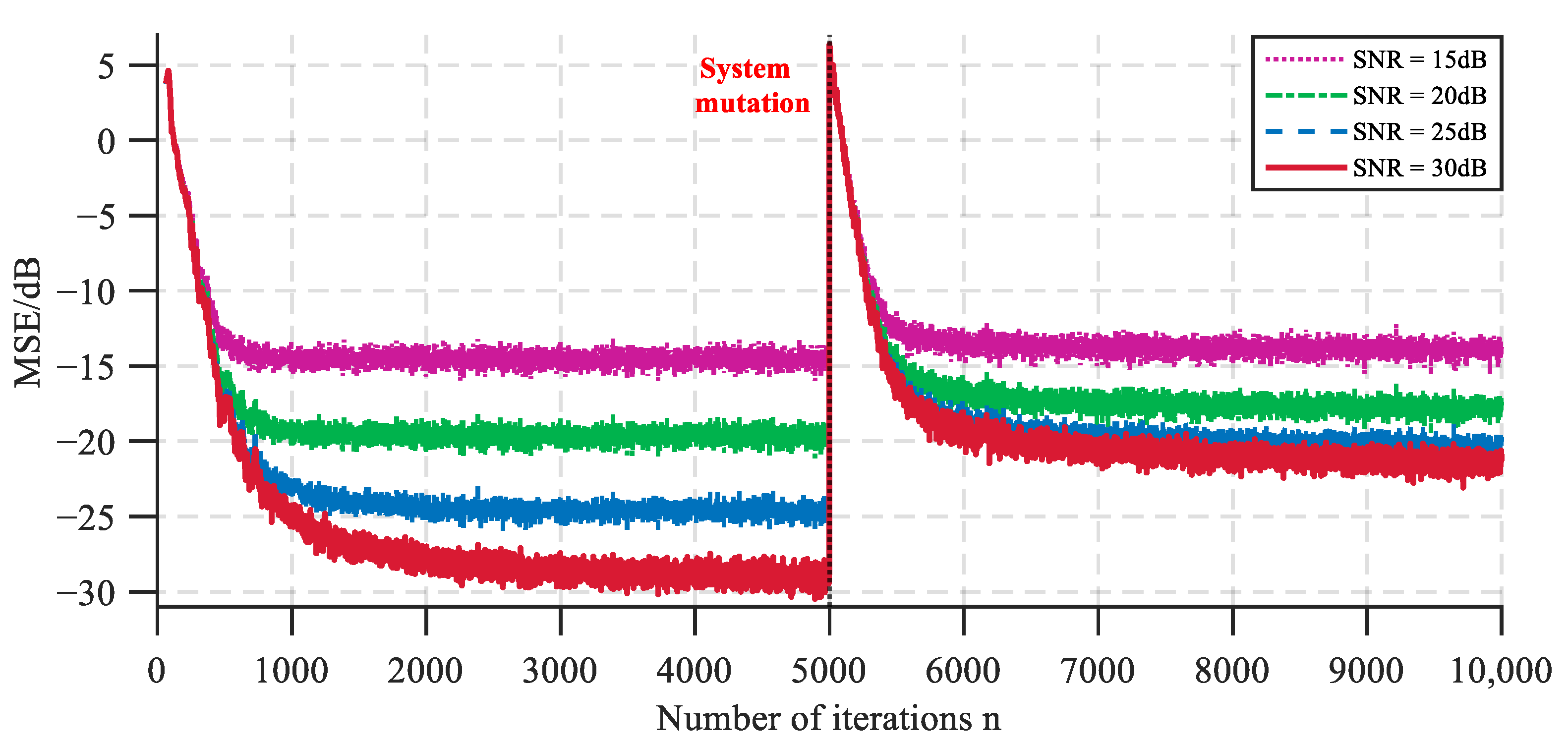
To evaluate the performance of the algorithm under different pulsation intensities, four noise environments are constructed by varying the signal-to-noise ratio parameter (15–30 dB), corresponding to the hydraulic system’s strong interference (15 dB), standard (20 dB, 25 dB), and low interference (30 dB) conditions. The simulation parameters remain consistent with Case I. Results are shown in Figure 5 and Figure 6.

Figure 5 demonstrates each algorithm’s performance under different SNR conditions, while Figure 6 specifically shows the proposed algorithm’s performance. The DNVSS-FxLMS algorithm exhibits strong adaptive convergence capability across all SNR conditions. Overall, steady-state MSE values vary significantly among variable step-size algorithms as SNR changes. The proposed algorithm’s steady-state MSE decreases with increasing SNR, showing progressively greater performance advantages over other algorithms. From Figure 5, we can see that when the signal-to-noise ratio is 15 dB, the MSE of the four variable step-size algorithms remains basically consistent. However, when the signal-to-noise ratio increases to 30 dB, the steady-state error of the proposed algorithm can reach −29.4 dB, which is 5–7 dB better than other variable step-size algorithms. This result verifies Theorem 2 in Section 4, Performance Analysis: the DNVSS-FxLMS algorithm achieves ultralow steady-state error in high-SNR environments where misalignment decreases cubically.

5.3. Case 3: Periodic Load Changes

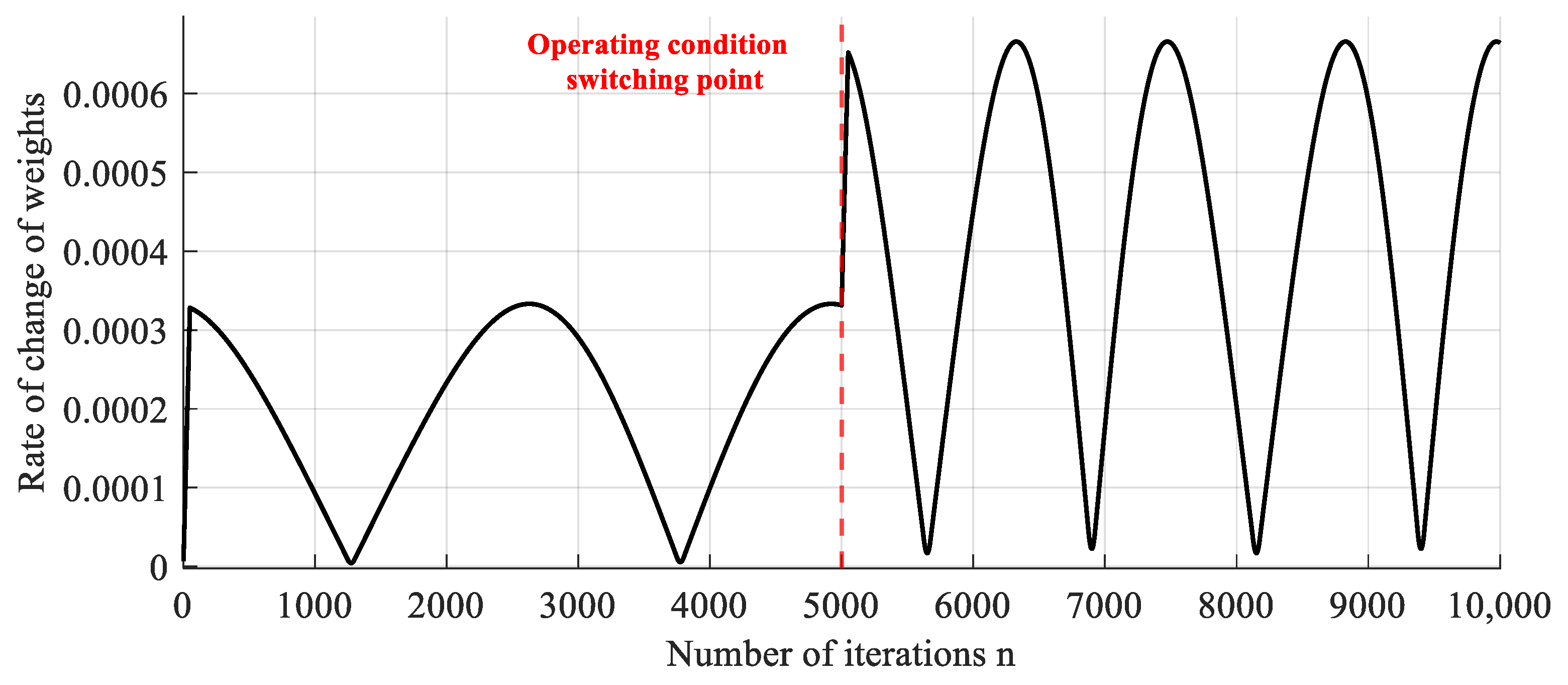
In order to verify the effectiveness of the proposed algorithm under the working conditions of dynamic load changes in the hydraulic system, this case constructs a periodic load change model to simulate scenarios such as the cyclic process of the injection molding machine and the periodic excitation of the hydraulic vibration table, and requires that the control algorithm can stably track such regular changes. System weights follow the oscillatory distribution in Equation (45), modulated by a sinusoidal function to reflect cyclic parameter changes caused by load, flow rate, temperature, and other operating factors. The model switches conditions at 5000 iterations, with weight coefficients changing cyclically (T = 5000 and T = 2500). Results are shown in Figure 7 and Figure 8.

Figure 7 demonstrates the system weights rate of change curve, in which the weights rate of change varies periodically with the number of iterations, and at the working condition switching point (n = 5000), the rate of change shows an obvious discontinuity, with the amplitude nearly doubled. From the MSE curves in Figure 8, it can be seen that the DNVSS-FxLMS algorithm consistently maintains the lowest steady-state error and fast convergence rate throughout the simulation. The proposed algorithm exhibits the smallest steady-state mean square error fluctuation amplitude when the system parameters undergo periodic changes, which fully verifies the robustness of the algorithm. In contrast, the other algorithms exhibit larger mean square error fluctuations and slower convergence rates. It is worth noting that at the operating condition switching point (n = 5000), the DNVSS-FxLMS algorithm is able to complete the transition with the lowest mean-square error fluctuation, although the rate of change of the weights undergoes a large abrupt change.

Combining Figure 7 and Figure 8, based on the correlation between the MSE curve and the system weight change rate curve, it can be found that several algorithms exhibit different degrees of time lag effects. In

Table 5. Performance comparison of different algorithms under periodic load changes.

Algorithm	Peak Point of Weight Change Rate (n = 2639)			Peak Point of Weight Change Rate (n = 6329)
	Completed Tracking Points	Tracking Speed	MSE (dB)	Completed Tracking Points	Tracking Speed	MSE (dB)
FxLMS	3221	582	−10.0	6683	354	−9.0
VSSFxLMS-1/ Wang	2908	269	−12.6	6545	216	−10.7
VSSFxLMS-2/ Qian	2938	299	−13.0	6544	215	−11.3
VSSFxLMS-3/ Zhang	2864	225	−15.6	6484	155	−13.5
DNVSS-FxLMS	2674	35	−18.1	6416	87	−15.8

, a peak point of weight change rate was selected in each of the two stages to compare the convergence speed and steady-state error of various algorithms. For example, when the rate of change of weights peaks at n = 6329, the DNVSS-FxLMS algorithm completes the tracking after 87 iterations; however, the VSSFxLMS-3, which performs better, requires 155 iterations to reach the new steady-state, and the fixed-step FxLMS algorithm takes longer. Therefore, the tracking performance of the proposed algorithm is significantly better than that of other algorithms, while always maintaining a steady-state error that is 2–8 dB lower than that of other algorithms.

In the table, the completed tracking points represent the points where the algorithm re-converges after the system weights reach the peak point, achieving the tracking of weight changes. The tracking speed refers to the difference between the completed tracking point and the peak point of the weight change rate, directly reflecting the tracking ability of the algorithm for time-varying systems.

In summary, under the periodic variation of the load, the DNVSS-FxLMS algorithm is significantly superior to other algorithms in terms of convergence rate, steady-state error, and tracking performance.

5.4. Case 4: Unstable Random Load Changes

In the actual hydraulic system, factors such as the collaborative operation of multiple actuators, random external disturbances, and nonlinear load characteristics are superimposed. System parameters may exhibit irregular change characteristics that are difficult to fully simulate through periodic models. To evaluate the DNVSS-FxLMS algorithm’s performance in realistic operating conditions, a three-frequency irregular load model is constructed. This model simulates complex scenarios, including multi-load coupling in hydraulic pumping stations, composite actuator motions, and simultaneous external disturbances. The system weight distribution (Equation (44)) is co-modulated by three sinusoids (T₁ = 3500, T₂ = 2500, T₃ = 1000; A₁ = 0.40, A₂ = 0.25, A₃ = 0.15). Results are shown in Figure 9 and Figure 10.

Figure 9 reveals irregular fluctuations in system weight change rates, with multiple significant peaks during iterations. Figure 10 demonstrates algorithm convergence differences: the DNVSS-FxLMS algorithm achieves fastest initial convergence and maintains minimal steady-state error throughout. This dynamic uncertainty poses a serious challenge to the tracking performance of the algorithm when the system parameters are in a complex environment with irregular variations.

Table 6. Performance comparison of different algorithms under unstable random load changes.

Algorithm	Peak Point of Weight Change Rate (n = 4456)			Peak Point of Weight Change Rate (n = 7415)
	Completed Tracking Points	Tracking Speed	MSE (dB)	Completed Tracking Points	Tracking Speed	MSE (dB)
FxLMS	4720	264	−10.4	7616	201	−11.5
VSSFxLMS-1/ Wang	4600	144	−10.1	7570	155	−12.8
VSSFxLMS-2/ Qian	4598	142	−10.2	7569	154	−12.8
VSSFxLMS-3/ Zhang	4551	95	−11.6	7516	101	−14.4
DNVSS-FxLMS	4500	44	−13.6	7475	60	−16.4

presents the comparison of the tracking speed and steady-state error at the peak point of the weight change rate. It can be seen that the DNVSS-FxLMS algorithm has improved the convergence speed by at least double. Meanwhile, the MSE is always 2–5 dB lower than that of other algorithms, demonstrating significant dynamic tracking advantages and superior control effects.

In the environment of unsteady stochastic systems, the DNVSS-FxLMS algorithm shows significant advantages in terms of mean square error, convergence rate, and tracking ability based on its unique dynamic adaptive step-size adjustment strategy. The algorithm can effectively adapt to the complex time-varying process of a hydraulic system, and has excellent disturbance adaptation capability and robustness, which can be reliably applied in the active control system of hydraulic system pressure pulsation that requires real-time tracking control.

In unsteady stochastic environments, the DNVSS-FxLMS algorithm demonstrates significant advantages in mean squared error, convergence rate, and tracking ability through its unique dynamic adaptive step-size adjustment strategy. The algorithm effectively adapts to complex time-varying processes in hydraulic systems, exhibiting excellent disturbance adaptation and robustness. These features allow for reliable applications in active systems that require real-time tracking and control of pressure pulsations in hydraulic systems.

6. Conclusions

In this paper, a novel coupled variable step-size FxLMS algorithm is proposed, which couples the properties of two nonlinear functions, namely, rational fraction and exponential functions. The variable step-size strategy endows the algorithm with high convergence rate at the initial stage, low steady-state error in the steady-state phase, and stable tracking capability, thereby enabling its adaptation to the complex and variable control environment similar to that of a hydraulic system. Through simulation experiments, when the system undergoes unstable random changes, compared with traditional and existing variable-step algorithms, the convergence speed of the DNVSS-FxLMS algorithm is increased at least two-fold, and the steady-state error is reduced by 2–5 dB. The DNVSS-FxLMS algorithm exhibits both excellent adaptive convergence performance and significant comprehensive performance advantages over other variable step-size algorithms. The algorithm is robust to different signal-to-noise ratios and different dynamic characteristics. Notably, the performance advantages of the DNVSS-FxLMS algorithm become increasingly significant with the increase in signal-to-noise ratio or control system complexity, thus providing a solid foundation for its practical application in complex and variable hydraulic system control.

References

- Wang, Y.; Shen, T.; Tan, C.; Fu, J.; Guo, S. Research Status, Critical Technologies, and Development Trends of Hydraulic Pressure Pulsation Attenuator. Chin. J. Mech. Eng. 2021, 34, 14. [Google Scholar] [CrossRef]
- Wu, C.; Jiao, Z.; Xu, Y.; Li, C.; Liu, Q.; Wu, S. Active Control Method for Fluid-Borne Noise in Aerospace Fluid Systems of Variable Operation Statuses. Mech. Syst. Signal Process. 2024, 214, 111375. [Google Scholar] [CrossRef]
- Pan, M.; Hillis, A.; Johnston, N. Active control of fluid-bome noise in hydraulic systems using in-series and by-pass structures. In Proceedings of the 2014 UKACC International Conference on Control (CONTROL), Loughborough, UK, 8–11 July 2014; IEEE: Piscataway, NJ, USA, 2014; pp. 355–360. [Google Scholar] [CrossRef]
- Zhu, Y.; Zhao, H.; Zeng, X.; Chen, B. Robust Generalized Maximum Correntropy Criterion Algorithms for Active Noise Control. IEEE/ACM Trans. Audio Speech Lang. Process. 2020, 28, 1282–1292. [Google Scholar] [CrossRef]
- Pan, M.; Yuan, C.; Ding, B.; Plummer, A. Novel Integrated Active and Passive Control of Fluid-Borne Noise in Hydraulic Systems. J. Dyn. Syst. Meas. Control 2021, 143, 091006. [Google Scholar] [CrossRef]
- Aboulnasr, T.; Mayyas, K. A Robust Variable Step Size LMS-Type Algorithm: Analysis and Simulations. IEEE Trans. Signal Process. 2002, 45, 631–639. [Google Scholar] [CrossRef]
- Li, M.; Li, L.; Tai, H.M. Variable Step size LMS Algorithm Based on Function Control. Circuits Syst. Signal Process. 2013, 32, 3121–3130. [Google Scholar] [CrossRef]
- Bismor, D.; Czyz, K.; Ogonowski, Z. Review and Comparison of Variable Step Size LMS Algorithms. Int. J. Acoust. Vib. 2016, 21, 24–39. [Google Scholar] [CrossRef]
- Mikhail, W.; Wu, F.; Kazovsky, L.; Kang, G.; Fransen, L. Adaptive Filters with Individual Adaptation of Parameters. IEEE Trans. Circuits Syst. 1986, 33, 677–686. [Google Scholar] [CrossRef]
- Kwong, R.H.; Johnston, E.W. A Variable Step size LMS Algorithm. IEEE Trans. Signal Process. 1992, 40, 1633–1642. [Google Scholar] [CrossRef]
- Zhao, Y.; Lin, L.; Dong, W.; Wang, H.; Wu, Z.; Wang, X.; Chen, X. A New Variable Step Size LMS Method and Its Application in DOA Estimation of OFDMA Signals. J. Southeast Univ. 2020, 36, 145–151. [Google Scholar] [CrossRef]
- He, D.; Wang, M.; Han, Y.; Hui, S. Variable Step size LMS Adaptive Algorithm Based on Exponential Function. In Proceedings of the 2019 IEEE International Conference on Information Communication and Signal Processing (ICICSP), Weihai, China, 28–30 September; IEEE: Piscataway, NJ, USA, 2019; pp. 473–477. [Google Scholar] [CrossRef]
- Bin Saeed, M.O.; Zerguine, A. A Variable Step Size Diffusion LMS Algorithm with a Quotient Form. EURASIP J. Adv. Signal Process. 2020, 2020, 12. [Google Scholar] [CrossRef]
- Luo, Z.; Zhao, H.; Zeng, X. A Class of Diffusion Zero Attracting Stochastic Gradient Algorithms with Exponentiated Error Cost Functions. IEEE Access 2019, 8, 4885–4894. [Google Scholar] [CrossRef]
- Yu, Y.; Zhao, H. An Improved Variable Step Size NLMS Algorithm Based on a Versiera Function. In Proceedings of the 2013 IEEE International Conference on Signal Processing, Communication and Computing (ICSPCC), Kunming, China, 5–8 August 2013; IEEE: Piscataway, NJ, USA, 2013; pp. 1–4. [Google Scholar] [CrossRef]
- Huo, Y.L.; Long, X.Q.; Lian, P.J.; Wang, D.L. A Variable Step Size Normalized Adaptive Filtering Algorithm Based on a Versiera-Like Function. J. Electron. Inf. Technol. 2021, 43, 335–340. [Google Scholar] [CrossRef]
- Kumar, K.; Pandey, R.; Bora, S.S.; George, N.V. A Robust Family of Algorithms for Adaptive Filtering Based on the Arctangent Framework. IEEE Trans. Circuits Syst. II Express Briefs 2022, 69, 1967–1971. [Google Scholar] [CrossRef]
- Zeng, J.; Lin, Y.; Shi, L. A Normalized Least Mean Square Algorithm Based on the Arctangent Cost Function Robust Against Impulsive Interference. Circuits Syst. Signal Process. 2016, 35, 3040–3047. [Google Scholar] [CrossRef]
- Rosalin; Patnaik, A. A Filter Proportionate LMS Algorithm Based on the Arctangent Framework for Sparse System Identification. Signal Image Video Process. 2024, 18, 335–342. [Google Scholar] [CrossRef]
- Yang, L.; Liu, J.; Yan, R.; Chen, X. Spline Adaptive Filter with Arctangent-Momentum Strategy for Nonlinear System Identification. Signal Process. 2019, 164, 99–109. [Google Scholar] [CrossRef]
- Zhou, Y.; Zhang, Q.; Yin, Y. Active Control of Impulsive Noise with Symmetric α-Stable Distribution Based on an Improved Step Size Normalized Adaptive Algorithm. Mech. Syst. Signal Process. 2015, 56, 320–339. [Google Scholar] [CrossRef]
- Zhang, J.W.; Yu, H.; Zhang, Q.H. An Improved Variable Step Size LMS Algorithm Based on Hyperbolic Tangent Function. J. Commun. 2020, 41, 116–123. [Google Scholar] [CrossRef]
- Jalal, B.; Yang, X.; Liu, Q.; Long, T.; Sarkar, T.K. Fast and Robust Variable Step Size LMS Algorithm for Adaptive Beamforming. IEEE Antennas Wirel. Propag. Lett. 2020, 19, 1206–1210. [Google Scholar] [CrossRef]
- Zhang, J.R.; Zhang, T. An Improved Variable Step Size LMS Adaptive Filtering Algorithm. J. Xi’an Univ. Posts Telecommun. 2021, 26, 7–12. [Google Scholar] [CrossRef]
- Qian, M.N.; Lu, J.W.; Yan, G.X.; Guo, J.H. An Improved Variable Step Size LMS Algorithm for Vehicle Interior Noise Control. J. Hefei Univ. Technol. (Nat. Sci.) 2021, 44, 1306–1310. [Google Scholar] [CrossRef]
- Zhang, X.; Yang, S.; Liu, Y.; Zhao, W.; Ni, T. Improved Variable Step size Least Mean Square Algorithm for Pipeline Noise. Sci. Program. 2022, 2022, 3294674. [Google Scholar] [CrossRef]
- Li, L.; Zhao, X. Variable Step Size LMS Algorithm Based on Hyperbolic Tangent Function. Circuits Syst. Signal Process. 2023, 42, 4415–4431. [Google Scholar] [CrossRef]
- Jiang, J.; Gao, Z.; Zhang, H.; Zhu, X. Research on Active Vibration Control of Blade Using Variable Step Size Filtered-x Least Mean Square Algorithm. J. Vib. Control 2024, 31, 2464–2477. [Google Scholar] [CrossRef]
- Elliott, S.J.; Nelson, P.A. Active Noise Control. IEEE Signal Process. Mag. 1993, 10, 12–35. [Google Scholar] [CrossRef]
- Wang, C.; He, L.; Li, Y.; Zhang, X.; Zuo, L. An Anti-Interference Variable-Step Adaptive Algorithm and Its Application in Active Vibration Control. In Proceedings of the 2016 IEEE/OES China Ocean Acoustics (COA), Harbin, China, 9–11 January 2016; IEEE: Piscataway, NJ, USA, 2016; pp. 1–5. [Google Scholar] [CrossRef]
- Sayed, A.H. Adaptive Filters; John Wiley & Sons: Hoboken, NJ, USA, 2011. [Google Scholar]