3.1. Problem Description
The swarm robot system enters the region through self-organization mode for the unknown environment. The system is initially in a state of random and uneven distribution. To adapt to the pattern of the region, a rapid regional adaptive adjustment mechanism enables the robots to distribute over the area evenly. In the case of an area that is changing rapidly, the swarm robots must be able to adapt quickly to ensure uniform coverage.
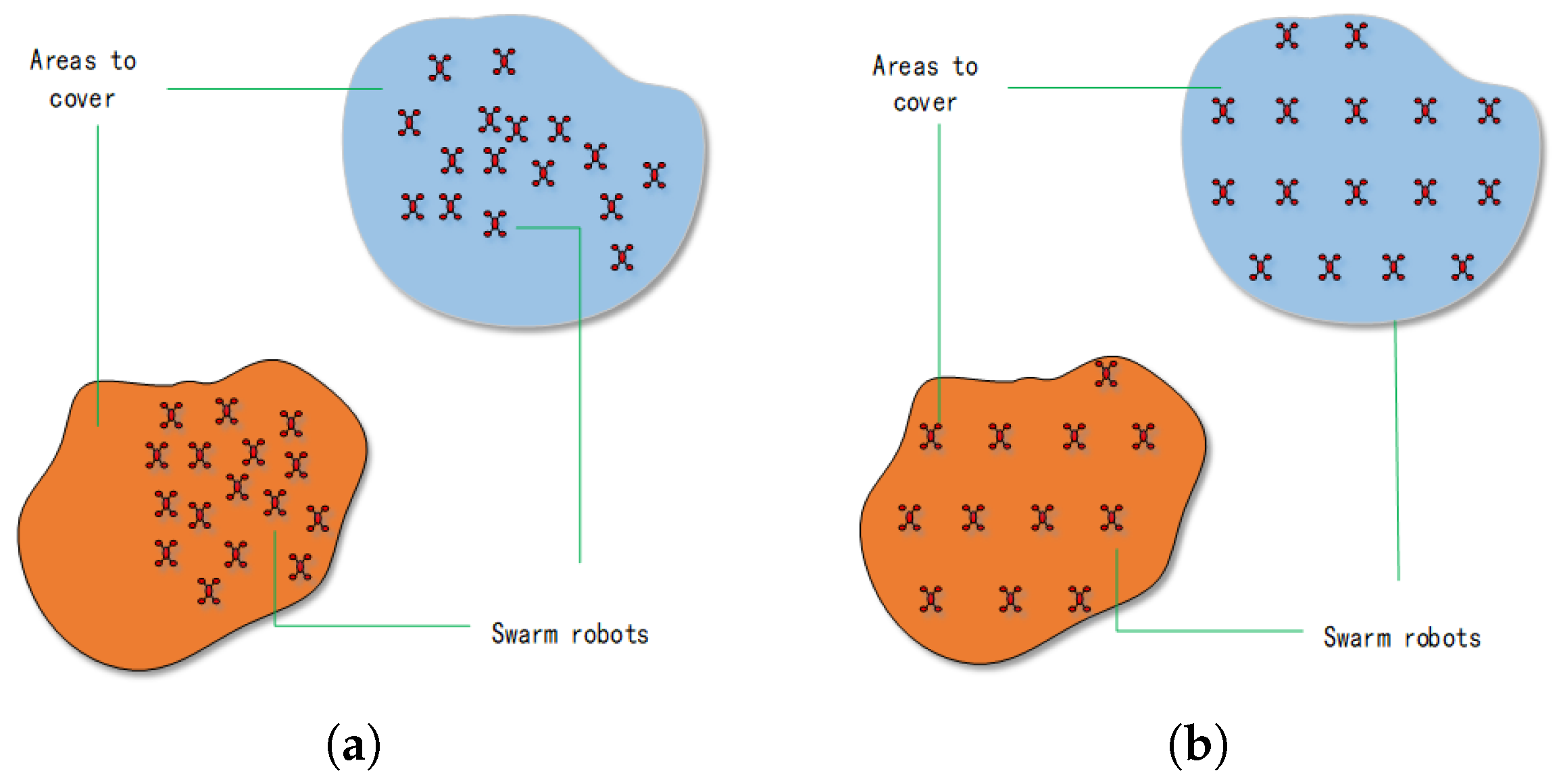
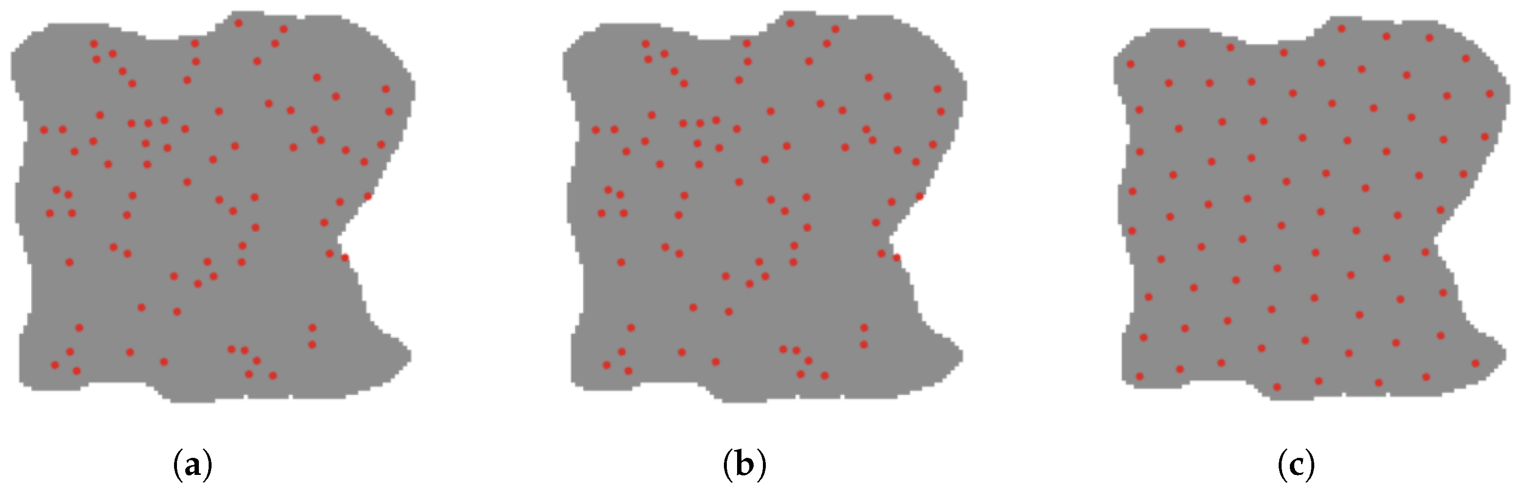
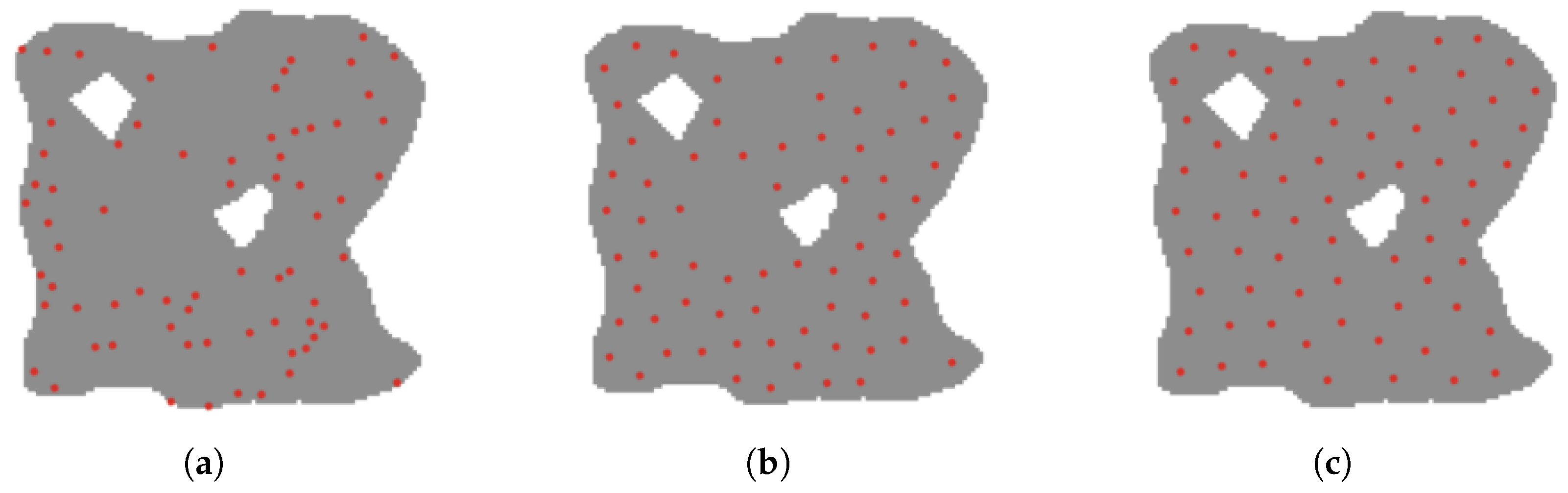
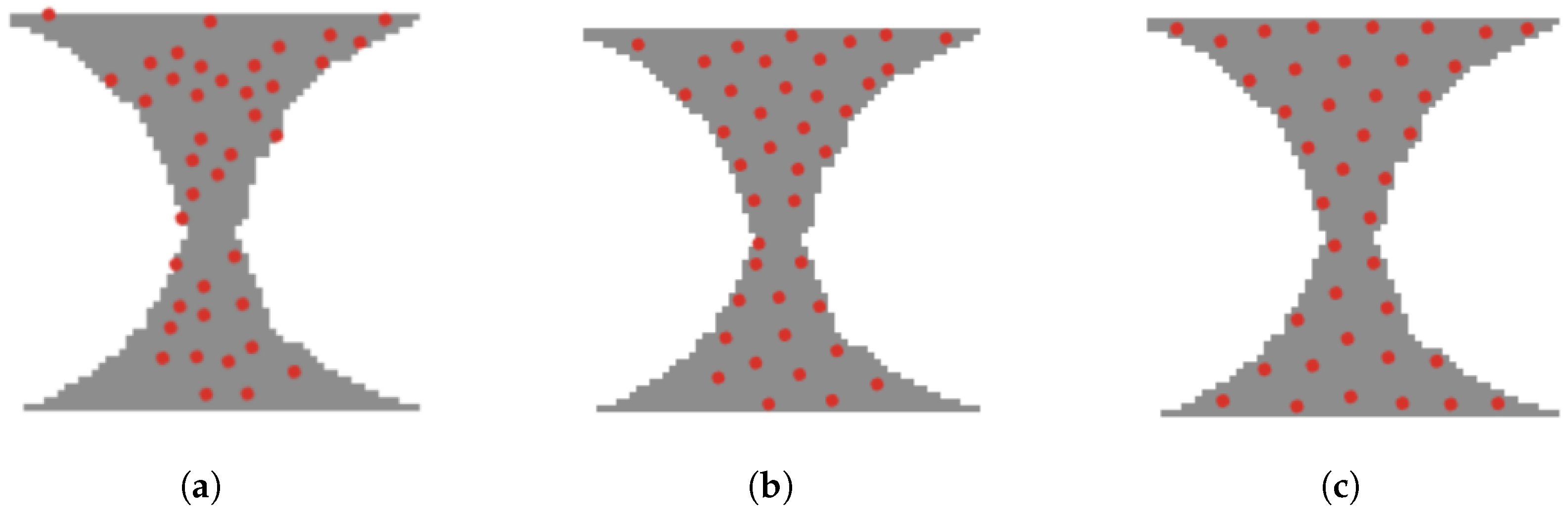
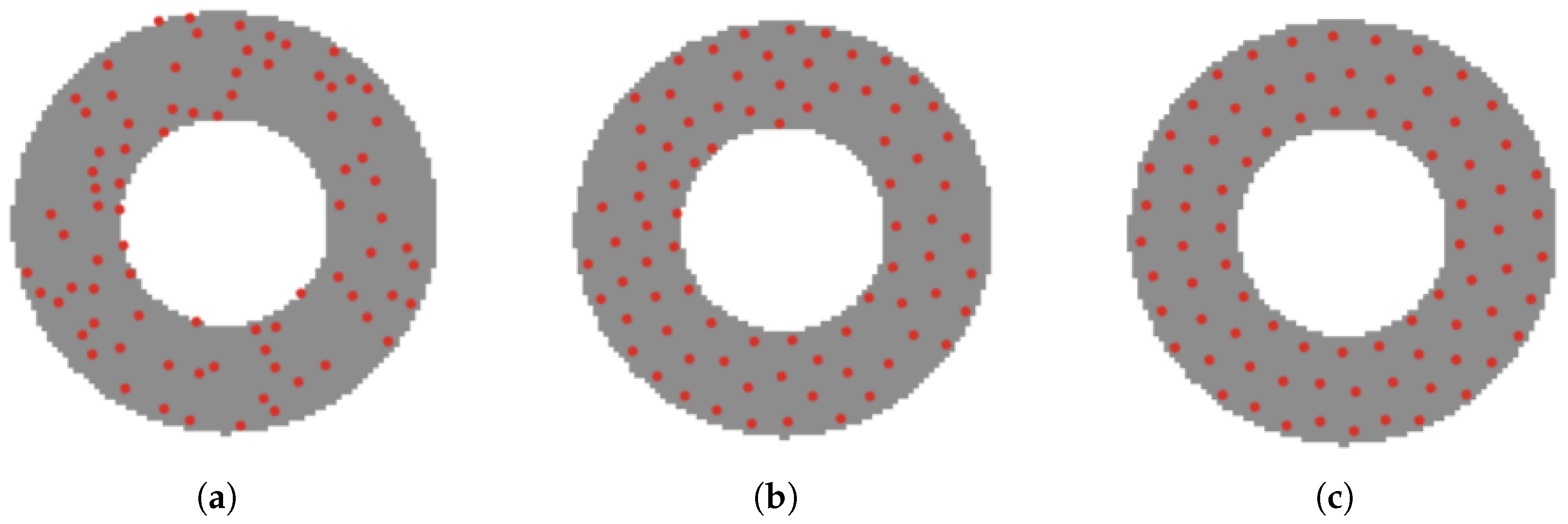
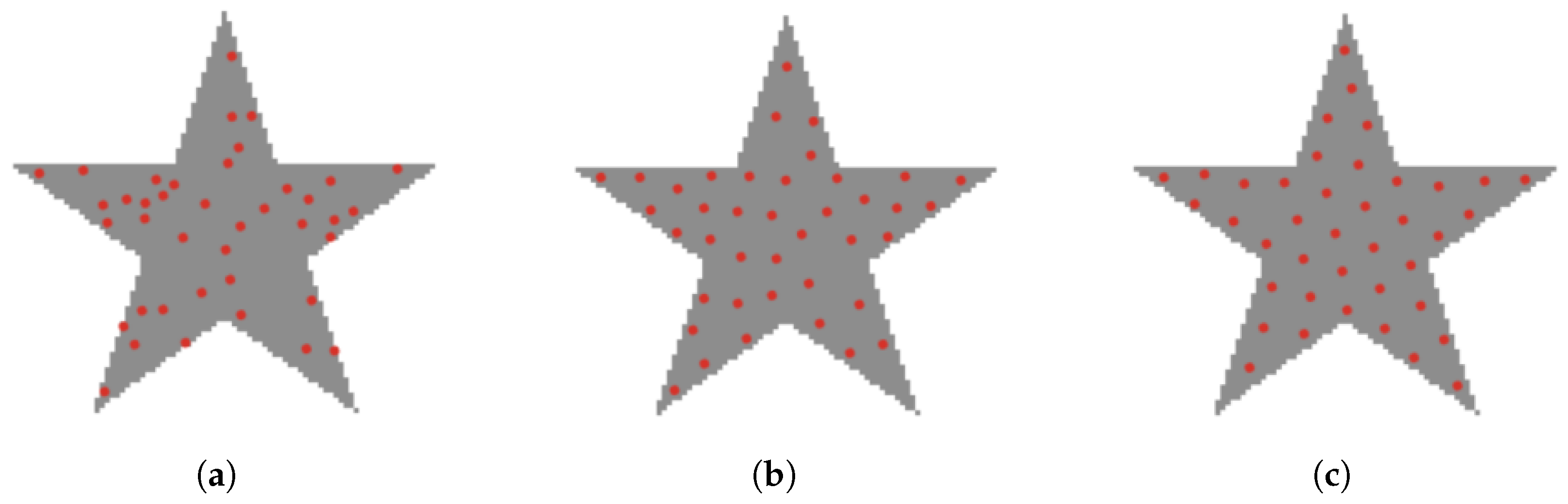
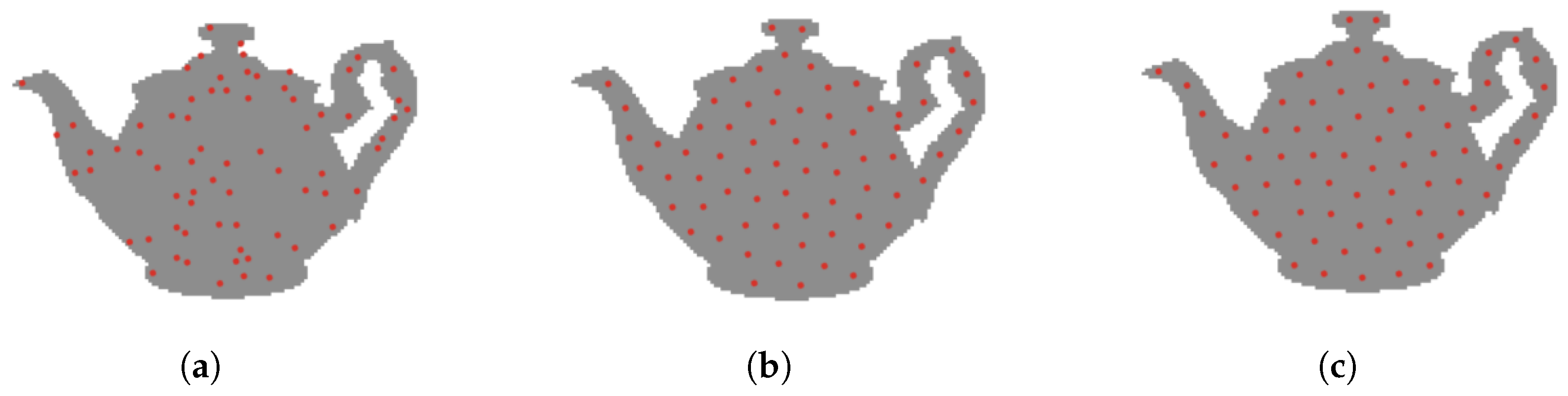
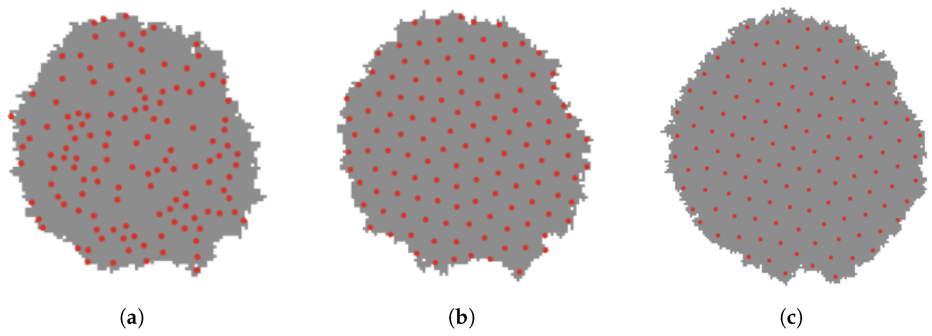
Figure 1 shows the scene of covering tasks in various areas of the swarm robots.
Figure 1a shows the initial distribution of the swarm robots system in the required coverage area, and the robots do not cover the area uniformly.
Figure 1b shows the adjusted distribution of the swarm robots after the adjustment of the intra-regional adaptive mechanisms.
Definition 1 (Swarm robotic system). A swarm robot system is a system consisting of n robots, which we define as , where denotes an individual robot. Each individual robot can be described by a six-tuple . Where x represents the position of the robot and where the robot is regarded as a point with no shape or size, so x represents the coordinates of the point where the robot α is currently located. v represents the velocity vector of the robot α. represents the expected distance of the DVF of the robot α, that is, the distance that the robot α expects the surrounding robots to maintain. represents the maximum perception distance of the robot α, which means the range of information collected by a single robot, including the distribution of the target area within the range and other robot information. is used to indicate whether the individual robot has reached a state of convergence. represents the DVF vector perceived by the robot α.
In order to study the problem of adaptive uniform coverage based on dynamic virtual forces, in a swarm robot system, we define the control commands for each robot as follows:
A Robot should be able to perceive each other within a certain range.
For the neighbor robots that can be perceived, the distance and orientation relative to itself can be obtained.
Each robot should be able to perceive the state of the surrounding area within a certain range, that is, to be able to distinguish the difference of pixels in different areas.
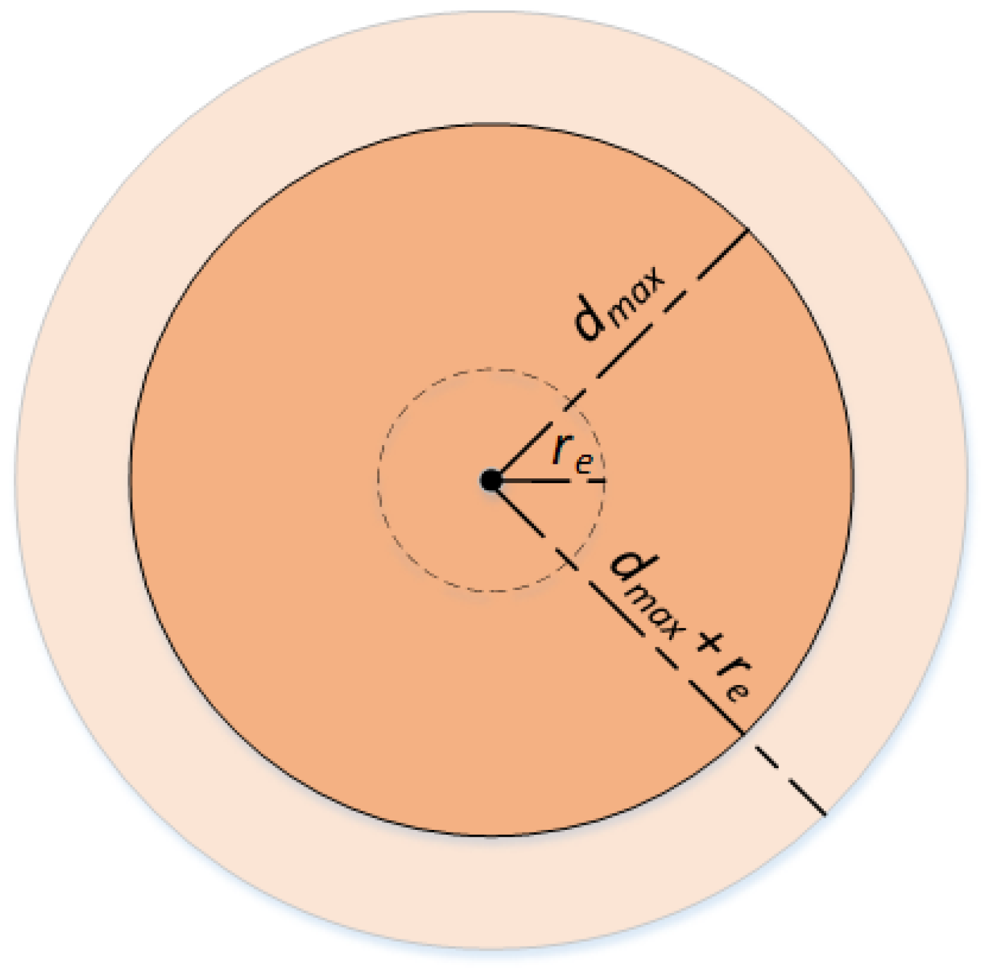
Because robots are able to move, when the number of robots is not enough to cover the target area, the robots must be able to move themselves to patrol the surrounding areas, which means that the coverage area will be expanded to a certain extent. Assuming that the patrol radius of robot α is , the maximum coverage radius of robot α is , as shown in Figure 2. To further supplement Formula (1), for a certain pixel and a certain body robot α in the area, the definition of whether the pixel is covered by the individual robot α is updated to Formula (1).
Definition 2 (Cover state
C)
. Let each robot be able to perceive the maximum distance (or the radius of the task that can be processed) as so the coverage area of the robot is . The environment is composed of a series of pixel point sets . For a certain pixel point and a certain body robot α, whether the pixel point is used by the individual robot α. The coverage is defined as Formula (2).where is the distance from robot α to . If the position of the robot is then Definition 3 (Coverage density
T)
. The number of robots in the area D to cover is , so the number of robots per unit area in the area is the coverage density of the area, defined as Formula (3). In some practical applications, the number of robots required varies depending on the mission requirements, such as cleaning up oil pollution in the ocean, where areas with high levels of pollution require more robots. In this case, we divide the region into n sub-regions with densities of according to the demand, and high-density areas tend to require more robots. Definition 4 (Four Neighbors N). The environment is a set composed of a series of continuous points, and each point can be described by a two-tuple . Among them, represent the coordinate position of in the two-dimensional plane space. Define each point in the area as the four-neighborhood N of this point, namely , where , that is, the four points at the top, bottom, left, and right positions of point .
Definition 5 (Area Boundary
)
. In the four-neighborhood of any point in the definition area, the set of points that do not belong to the area D can be judged as the area boundary, namely: Problem 1. With a given number of swarm robots, identify a method that enables the robots to complete coverage tasks in unknown areas in a self-organizing manner, while maintaining a certain distance between each robot.
Under the condition that all robots do not reach , that constant velocity is always maintained, and that the robots can move in any direction, the distance of the robot to complete the coverage task is one of the objects we need to optimize. The robots do not know the target area at first, which means that the shape of the target area is not clear, and there may even be obstacles in the area. In the deployment process, each robot can only perceive its local environment and formulate its own motion strategy according to its local interaction. In order to ensure that the swarm robots are as uniform as possible in the area, we must optimize the ideal distance between the robots.
For
n robots, the optimization objective is determined according to Equations (5) and (6).
where
M represents the total moving distance of the robot.
and
represent the positions of robot
and robot
respectively;
d represents the ideal distance between robots, and
represents the neighbor node set of robot
.
Problem 2. For sub-regions with different densities in the target area, a method that can deploy a corresponding number of robots in different densities areas is determined.
Areas with different densities have different priorities. Areas with higher densities have higher priorities, and more robots need to be deployed. For sub-regions with different densities with unknown shapes in the target area, deploying a corresponding number of robots is a difficult problem.
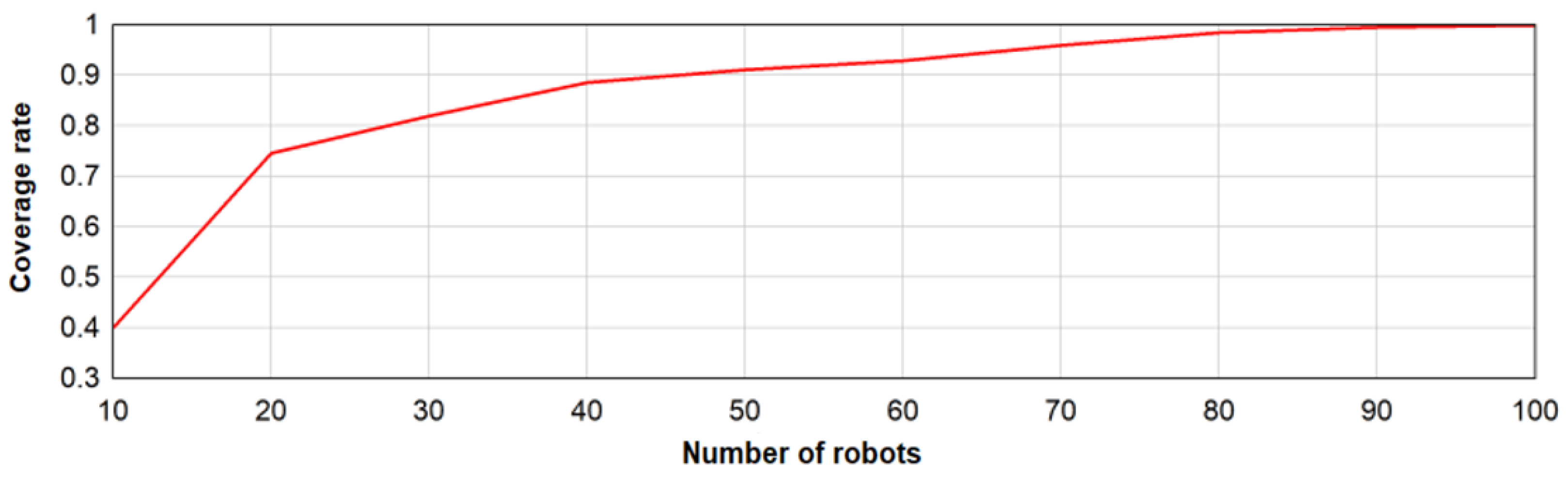
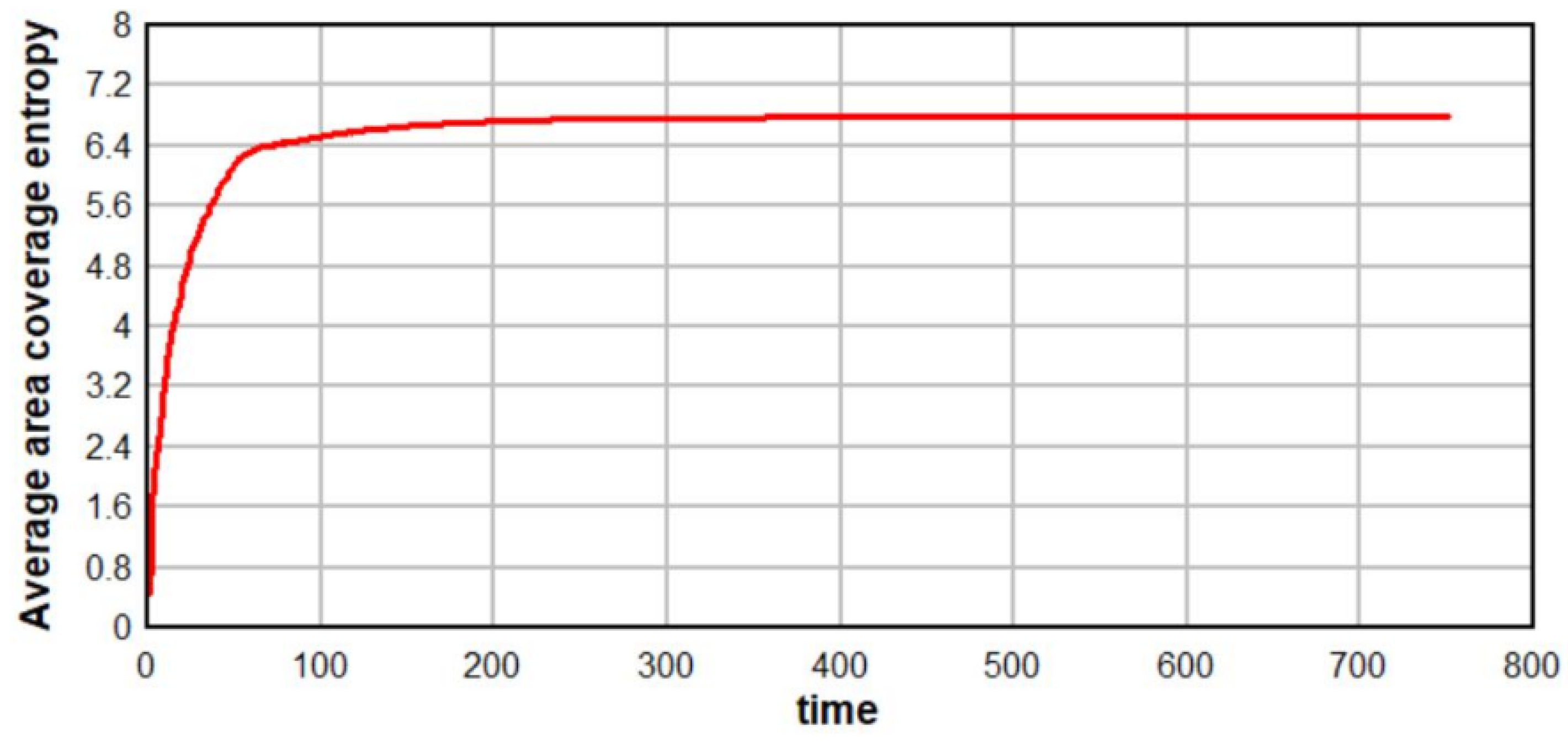
In this section, the formulas of the proposed method are related to the algorithms. We use three indicators to evaluate the performance of completing tasks: (1) the coverage rate based on robots’ final positions, (2) the uniformity based on the robots’ final positions, (3) the total distance the robots moved. Our ultimate goal is that the swarm robots will maximize the coverage area uniformly.
3.2. Adaptive Adjustment of Adjacent Distance
Assuming that the robots enter the designated area from any direction, the distribution of the robots after entering the designated area is not uniform at the beginning. For the uneven distribution of the robots, we can easily give an indicator of whether the area is uniform. The macroscopic non-uniformity for a single robot is the anisotropy of the number of surrounding robots, that is, if there are more robots in a certain direction, the robot should be far away from this direction, otherwise, the robot should be closer to this direction.
We propose a method of dynamic equalization of virtual force, which prompts the robot to move in the direction that will eliminate anisotropy. Assume that the set of robot
within perceptible distance
is
. The distance between robot
and a certain robot
in the robot set
is
, and the average
of the distance between
and all the robots around it is defined as Formula (7).
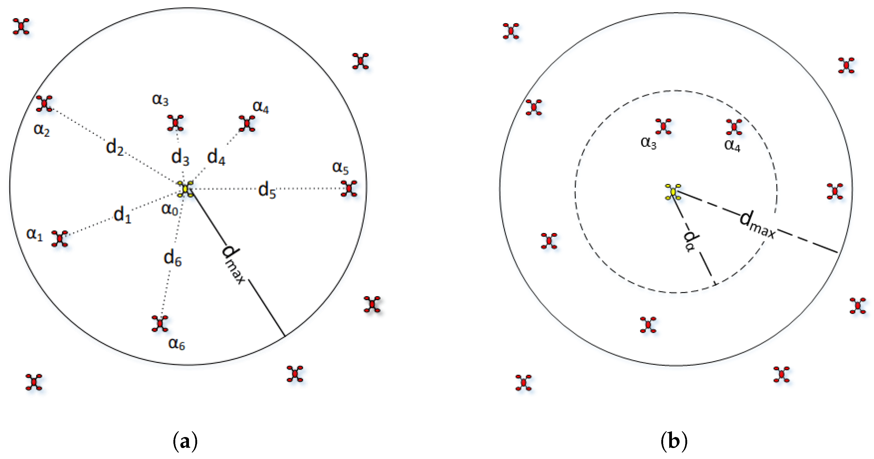
The distance relationships between each robot and its neighboring robots are shown in
Figure 3. Intuitively,
represents the minimum distance between
and the surrounding robot
, and it is also the DVF range of the individual robot. Let
be the distances from
to
, it can be seen from
Figure 3 that only two robots are in the range of
, which means that only these two robots will produce a virtual repulsive force towards robot
.
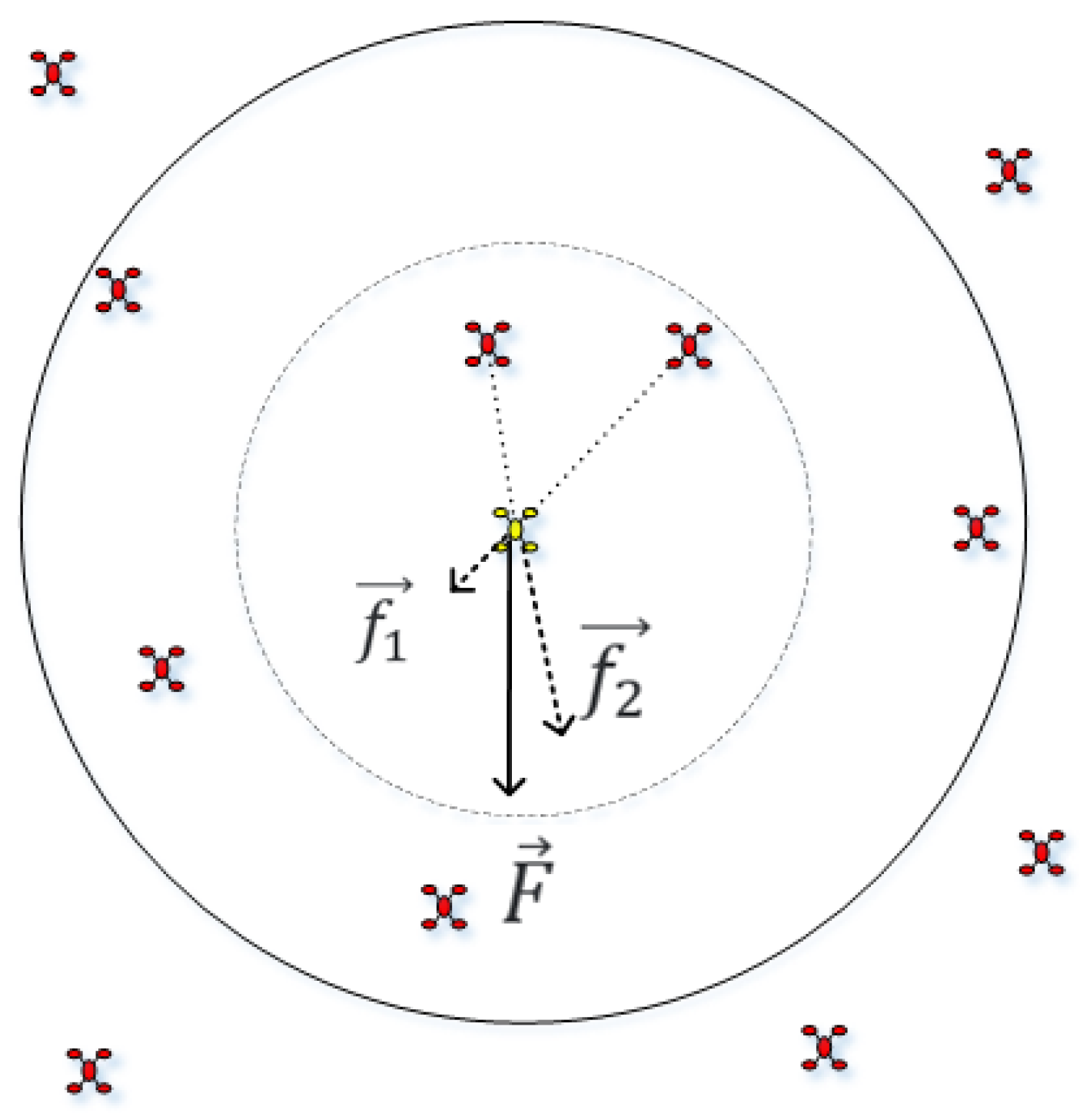
3.3. Interaction Scheme of Swarm Robots Based on Virtual Force
The resultant force generated by all the robots
is
to drive the robot
to move, as shown in
Figure 4.
Driven by the goal of expecting to maintain an average distance
from all surrounding robots, once the distance between the robot
around robot
and
is less than
, a corresponding virtual repulsive force
is generated by robot
, and the vector
means that
means the force of
on
in the x-axis direction, and
means the force of
on
in the y-axis direction. The specific calculation of the virtual force between robots is shown in Formula (8).
where
is the angle between the vector from
to
and the positive half-axis of the
x, and the direction of
is from
to
; and
is average distance of robot
; and
is a scaling coefficient that stabilizes boundary interactions by preventing excessive repulsive forces from expelling robot
beyond the area boundary. Obviously, the closer the robots are, the greater the virtual repulsive force generated. When the distance of all other robots within the expected distance
of robot
is equal to
, the virtual force
received by robot
is zero. Through this DVF, the distribution of the robot
and the surrounding robots becomes uniform. In the entire swarm robot system, each robot adjusts the distance between neighbors adaptively under the action of the mechanism described, so all of the robots are evenly distributed. This design embodies two critical sensitivities:
- 1.
Force Coefficient : Scales the repulsive force magnitude. Larger a (e.g., ) accelerates swarm dispersion but risks boundary overshoot, while smaller a (e.g., ) stabilizes motion at the cost of delayed convergence.
- 2.
Distance Threshold : Defines the effective repulsion range. Increasing enhances collision avoidance in dynamic environments, whereas decreasing optimizes dense formations but risks local congestion.
Through this adaptive DVF mechanism, robots dynamically adjust spacing to achieve uniform distribution. The logarithmic force model ensures repulsive intensity grows exponentially as , balancing global coverage with local collision avoidance.
Additionally, when the robot is in the range where it can perceive the area’s boundary, several points can be extracted from the boundary of the area within the perceptive range of the robot, and a virtual repulsive force is generated for the approaching robot through these boundary points. The boundary of the area can restrain all the robots in its range. Each robot uses the closest point in its perception boundary to generate a boundary force point, and each boundary point can only act on the robot that is closest to it, as shown in
Figure 5.
The repulsive force
generated by the boundary point
p on the robot
is calculated as shown in Formula (9).
where
is the angle between the vector from
p to
and the positive half axis of the x-axis, the direction of
is from
p to
, and
a is a constant between 0 and 1. Therefore, the resultant force experienced by each robot is shown in Formula (10).
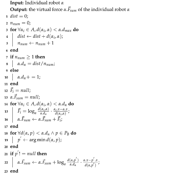
The calculation of the DVF directed towards by robot is shown in Algorithm 1.
First, the number of robots in the robot set around the robot is initialized and the average distance between the robot and the surrounding robots (lines 1–2), scan the swarm robots within the perception range of the individual robot, and update the values of and (lines 3–6). If the number of surrounding swarm robots is greater than or equal to 1, then update the dynamic virtual force range of the individual robot (lines 7–11). Then initialize the value of the virtual force and the resultant force (lines 12–13), scan the swarm robots in the dynamic virtual force range of the individual robot , and calculate the value of each swarm robot to the individual robot virtual force, and calculate the virtual force vector and (lines 14–17) generated by all the surrounding swarm robots, and scan the nearest boundary point in the dynamic virtual force range of the individual robot (lines 18–20). When there is a boundary point in the DVF range of the individual robot , calculate the virtual force of the boundary point for the individual robot , and update the virtual force resultant force (lines 21–22).
It is easy to calculate the total force direction
of the robot through
, so the position of the robot can be easily updated by using the kinetic formula, as shown in Formula (11).
where
is the updated position of the robot after time
t, and
is the current position of the robot.
When the target area changes, the local area may increase or decrease. We adopt a random spreading mechanism for each boundary set
point. Its four neighbors
. Points in the target area
all have a certain probability to randomly add to the target area, so as the area changes, the virtual forces on the robot will change accordingly and the robots in the whole area will be redistributed evenly.
| Algorithm 1: Dynamic virtual force update algorithm |
![Symmetry 17 01202 i001]() |
3.4. Adaptive Coverage Based on Different Densities
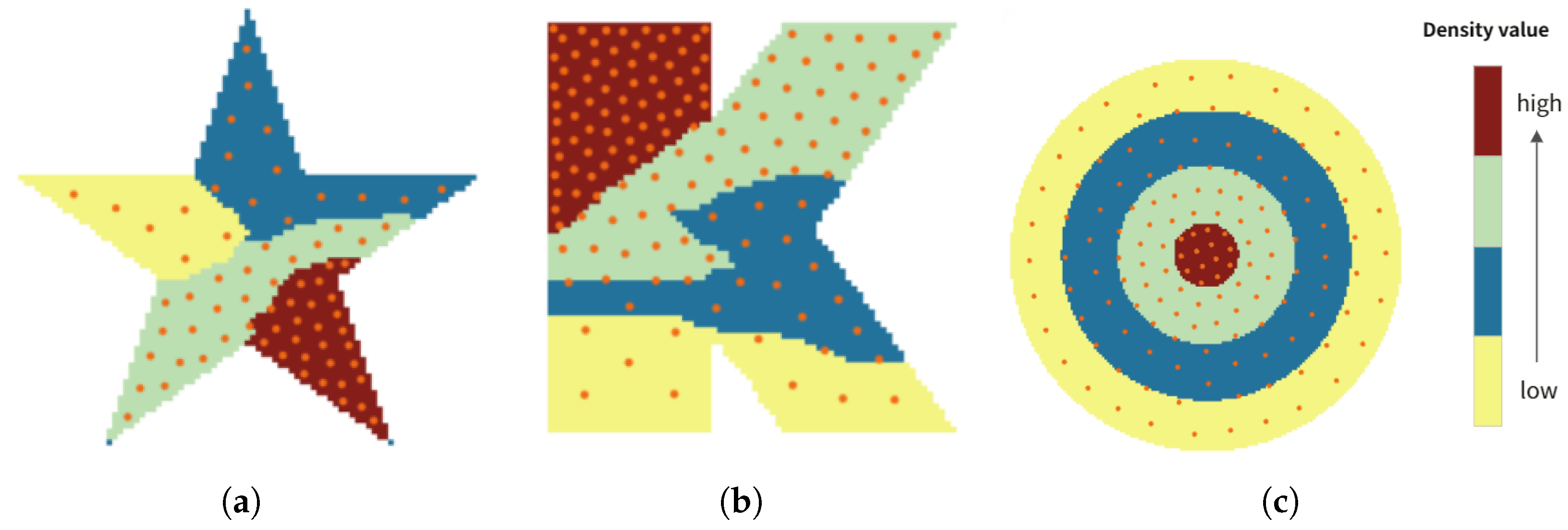
When swarm robots cover a task area, the number of robots needed at different locations in the area may be different, and we divide the area into multiple sub-regions with different densities according to the task requirements of the robots. High-density areas have higher priority than low-density areas, and high-density areas tend to require more robots to cover than low-density areas.
To assign the appropriate number of robots to sub-regions of different density, it is necessary to set different dynamic virtual forces for different priorities. Because the force between robots in different density areas is directional, the force is directed from the low density area to the high density area, so the swarm robots will also tend to gather in the high density area, as shown in
Figure 6.
The virtual forces between robots in areas of different densities is
, where
is the density of the
i-th area, and
. Assume that the virtual force between robots in the first density area is
, The virtual force between robots in adjacent density areas is the one of the previous density
Times (
It is a constant set according to the needs of regional density), then the virtual force between robots in the
i-th density area is:
3.5. Convergence Analysis
Even in a static environment, it is not possible to achieve convergence by stopping the robot by making the combined force . In fact, when a large number of robots are driven by DVFs to move, it is impossible to let the virtual force vector sum directed towards the robot remains at 0, and even the threshold that tends to 0 is difficult to set, which causes all robots to oscillate. In a dynamic environment, changes in the environment or changes in the number of robots are likely to cause frequent adjustments of the swarm robot system and cause oscillations. Therefore, it is necessary to set reasonable convergence conditions to determine the coverage of the robot population, so as to make the system relatively stable.
Since it is difficult for a single robot to judge the global coverage, it is necessary to convert the global convergence judgment into the convergence judgment of each robot. The robot records its own historical movement to determine whether it converged in the current position, based on the individual convergence probability to determine the global convergence of the entire swarm robot system.
Suppose that the latest
q movement of robot
is recorded as:
,
is the
k-th movement of robot
before
. The historical displacement vector sum of the robot
is shown in Formula (13).
Obviously, when the robot has not reached a relatively stable state, the historical movement will be in a certain general direction, and after reaching a relatively stable state,
will oscillate without direction in a small range. Therefore, as the robot continues to reach a relatively stable state,
will tend to decrease. The convergence threshold is set to
, and when
, the robot
is in a stable state. If all robots in the swarm robot system meet the convergence state, the system is considered to be converged. The condition for system convergence is shown in Formula (14).
Therefore, the position update algorithm of the individual robot is obtained as shown in Algorithm 2.
When the movement of the individual robot
does not converge, that is, the value of
is false, the following loop is performed: first, set the value of the counter
to a constant
q, when each counter time is performed, the force on the individual robot
is updated (line 2, call Algorithm 2), and move in the direction of the resultant force (lines 3–5), if the difference between the position of the individual robot
and its historical position
is less than the threshold
, it is determined that the motion of the individual robot has converged, that is,
(lines 6–8), and the information of the individual robot
is updated (line 9). At the same time, the counter time is decreased by one unit (line 10).
| Algorithm 2: Individual robot location update algorithm |
![Symmetry 17 01202 i002]() |
3.7. Stability Analysis
In a swarm robot system, we wish to show that the swarm robot system can maintain stability during motion. Consider two neighboring points in the same direction, at time 0 and at time
t. Let the spacing between these two points be
and
respectively, and let the number of robots be
n. Then the Lyapunov exponent
of the system in the same direction can be defined as:
Since the dynamic behavior of the robots in a swarm robotics system will gradually converge to a stable state and the value of the Lyapunov function will continue to decrease over time, thus indicating that the energy of the system is decaying at each time step. So when the exponent of the Lyapunov function is strictly less than zero, then the system is considered stable.
We substitute Formula (11) into the calculation and set the following initial parameters:
is set to [−100, 100].
Time t is set to 20,000.
Substituting gives , this shows that the swarm robot system in our proposed algorithm is stable.


