Abstract
Swarm robots often need to cover the designated area to complete specific tasks. While robots possess local perception and limited communication capabilities, they struggle to handle coverage issues in dynamic environments. This paper proposes a self-organizing algorithm for swarm robots based on Dynamic Virtual Force (DVF) to cover dynamic areas. Robots in the swarm can locally perceive their surrounding robots and dynamically select adjacent ones to generate virtual repulsion, thereby controlling their movement. The algorithm enables swarm robots to be rapidly and evenly deployed in unknown areas, adapt to dynamic area changes, and solve the problem of symmetrical robot distribution during coverage. It also allows for adaptive coverage of different density areas, divided as needed. Experimental validation across 20 benchmark scenarios (including obstacles, dynamic boundaries, and multi-density zones) demonstrates that the DVF method outperforms existing approaches in coverage rate, total robot movement distance, and coverage uniformity. The results validate its effectiveness and superiority in addressing area coverage problems. By addressing these challenges, the DVF algorithm can be widely applied to forest firefighting, oil spill cleanup in the ocean, and other swarm robot tasks.
1. Introduction
With the development of artificial intelligence, research on swarm robot systems has attracted much attention [1]. Compared with a single robot, Swarm robots have the potential to complete more complex and challenging scenarios, such as forest fire fighting [2,3,4], ocean oil spill cleaning [5,6], environmental monitoring [7,8], disaster prevention [9,10], agricultural applications [11,12] and many other fields [13,14,15]. In the above applications, the coverage problem deserve special attention [16].
The coverage problems are generally classified into static coverage, dynamic coverage, and persistent coverage [17]. Static coverage focuses on optimal agent deployment for fixed environments [18], while dynamic coverage requires agents to adapt to environmental changes and maintain coverage efficiency [19]. Persistent coverage emphasizes periodic revisit of all areas through continuous movement [20]. Sensor networks have been used to monitor target areas before, but these sensors are often immobile, and even if they can move, they are difficult to apply in dynamic and unknown environments, which is classified as a static coverage problem. For the dynamic coverage problem, mobile robots are used to monitor dynamic environments. Robots must adapt to the area and form a corresponding pattern to achieve high coverage. Moreover, the robot needs to cope with various changes. For example, when obstacles appear in the area, robots need to avoid the barriers promptly; when the area’s shape is dynamic, the robot needs to adjust its position in real-time to adapt to the changes [21,22].
After meeting the requirements of maintaining a high coverage area, swarm robots also need to consider coverage uniformity. Each robot has a fixed patrol area. The higher the uniformity of area coverage, the smaller the area of patrol repeatedly covered by robots, which means that in the same area, the area coverage algorithm with high uniformity can complete the coverage task with fewer robots. In addition, there may be different sub-areas in an area that require different numbers of robots to complete coverage tasks. For example, swarm robots are used to clean up oil spills at sea. Different numbers of robots need to be deployed for the uneven distribution of oil, and more robots are required for areas with high densities to achieve higher cleaning efficiency.
According to the primary goal of the swarm robot area coverage algorithm, the traditional swarm robot system usually has the following main challenges in solving the area coverage problem:
- In the absence of global positioning, it is difficult for swarm robots to quickly achieve adequate coverage of unknown environments only through the local perception and the limited communication with surrounding robots [23,24].
- When the shape of the target area is diverse or dynamic, swarm robots have difficulty making timely adaptive adjustments [25].
- For the traditional adaptive area coverage method, it is challenging to ensure uniform coverage.
Given these challenges, we proposes an idea of Dynamic Virtual Forces (DVF) that robot is subject to virtual repulsions from other robots as well as forces from boundary pointing to it within its own perception range, so swarm robots are able to quickly disperse to achieve uniform area coverage by dynamic virtual forces among them. The main contributions of this paper are as follows.
- 1.
- Dynamic virtual exclusion mechanism: Each robot is only subject to the repulsive virtual force of a portion of the robots within its perception range, thus effectively and rapidly controlling the movement of all robots and covering the target area.
- 2.
- Adaptive coverage: When there are complex features such as angles and rings in the area, our algorithm can make the swarm robots cover the area evenly, and the robots can also make adaptive adjustments in time for the dynamically changing area.
- 3.
- Density adaptive allocation: Our algorithm solves the problem of assigning different numbers of robots in an area according to different task requirements.
The rest of the paper is organized as follows. In Section 2, we introduce and discuss the relevant literature on the how swarm robots cover an area. Section 3 explains how the DVF-based swarm robot system performs self-organized coverage, and verifies the convergence of the robots. The simulation and experiment process are introduced in Section 4. Finally, Section 5 concludes this article.
2. Related Work
The coverage of a swarm robot is the distribution of a group of robots in the environment. An important goal of the swarm robot algorithm is to maximize the coverage area while maintaining the communication distance between neighboring robots to keep the network fully connected. There are three standard methods for studying the coverage of swarm robots: the potential field method [26,27,28,29], the geometric method [30,31,32,33,34,35], and the biological heuristic method [36,37,38,39]. The potential-field-based method mainly controls the movement of robots by forming a potential field around the robot, which acts as an attractive or repulsive force to other robots. The geometry based methods are generally related to Voronoi diagrams, and the Voronina region of the robot is used to guide the robot to move to a more suitable position [40]. The biology-based heuristic method seeks inspiration from biological systems and uses the self-organizing behavior of organisms to achieve regional coverage.
The potential-field-based method is a collaborative control strategy that guides swarm robots through the area by constructing a virtual force field [26]. This force field contains attractive and repulsive forces, where the attractive force moves the robots towards the target area and the repulsive force avoids collisions between the robots. By computing the synthesized force field, the robots can choose the appropriate direction and speed of movement based on the forces perceived at their current position. The robot in this algorithm can instantly make decisions based on the perceived force field information and quickly adapt to environmental changes. However, if it is in a complex environment, the robot is prone to local minima and cannot find the optimal path, and the calculation of the force is more complicated, which will affect the execution speed of the robot.
Zou [27] proposed the virtual force algorithm (VFA) to build a sensor network with uniform deployment, using the VFA as a sensor deployment strategy, and used attraction and repulsive forces to determine the sensor’s virtual motion path and velocity until its final location was determined. But the algorithm failed to consider environmental obstacles and dynamic changes. Rout et al. [28] proposed the obstacle avoidance virtual force algorithm (OAVFA), considering the presence of obstacles and defining that they would exert a virtual repulsive force on the robot. However, only one obstacle shape was tested in the experiment, without considering different boundary or obstacle geometries. These traditional potential-field-based methods have a fast convergence rate but require an excellent mechanical model; otherwise, isolated nodes or oscillation may occur. Unlike these algorithms, the DVF method is a dynamic evolution of the potential field method, characterized by two key features. First, whereas predecessors rely on a combination of attractive and repulsive forces, DVF solely uses repulsive forces, simplifying the interaction model and enhancing deployment efficiency. Second, DVF adapts excellently to dynamic environments, enabling real-time force field adjustment based on changing robot positions and environmental conditions.
Geometry-based methods mainly rely on the Voronoi diagram. Nair et al. [30] proposed a Manhattan Voronoi Partition and Spanning Tree Coverage Collaborative Framework, which realizes synchronous swarm robot exploration and coverage in known structured environments, featuring high robustness and fault tolerance. Teruel et al. [31] developed a distributed self-deployment mechanism that enables robots to organize uniformly for dynamic region coverage, significantly improving system convergence via feed-forward action. Elmokadem [32] presented a Voronoi partition-based region control approach, restricting robot motions within dynamic regions using planned dynamics. Jorge et al. [33,34] showed that mobile nodes can converge to the Voronoi unit’s center of mass. These algorithms feature fast convergence and no oscillation, but require nodes with strong computing capabilities. The DVF method overcomes the uniformity defects of geometry-based methods through logarithmic force modeling.
Seongin et al. [36] proposed an artificial pheromone system (BAPS) inspired by biopheromone behavior. By simulating natural pheromone diffusion and volatilization, the system enables robot clusters to self-organize and coordinate without centralized control. It adapts to dynamic environments but struggles to support high-speed coverage tasks. Zhang [37] proposed the COGPSO algorithm, which enhances real-time multitarget coverage response via hierarchical optimization and diversity strategies, but high inter-node communication costs limit its large-scale use. The above biological heuristic methods typically require environmental information and centralized computation. As the number of agents or obstacles grows, the optimization problem’s dimension increases substantially, potentially decreasing optimization efficiency significantly.
The angular depth-first method [41,42] is used to find some specific geometric structures, such as “corner” or “hall,” and to guide the movement of the leader robot by specifying specific operations on these structures. This method requires that the obstacles surrounding the environment be connected.
For the dynamic coverage area algorithm, Yu et al. [43] proposed a dynamic coverage planning algorithm based on K-means (K-means-DCC), which uses the combination of sliding window clustering and distributed Laplacian control to improve the coverage efficiency of swarm robots in dynamic environments, and can calculate the optimal coverage position of intelligent units by relaxing the requirements of coverage objects. The algorithm has a good effect on uniform target coverage, but it is not suitable for processing uneven target coverage, which limits the application of complex scenes. Xiao et al. [44] introduced a distributed dynamic based on reinforcement learning (RL-DAC). The robot learns the dynamic process to obtain the global optimal coverage strategy. The robot can get the local optimal coverage strategy when the communication does not cover the entire target area.
Although various swarm robots’ coverage methods can run in a distributed manner and perform regional coverage tasks well, they still have some limitations: (1) Most algorithms do not cover uniformity well. (2) Some methods need to predict the shape and size of the covered area. (3) Most methods do not apply to dynamic environments. (4) Adaptive coverage with different coverage densities is not considered. (5) Some algorithms have good coverage, but the speed of coverage is not ideal.
3. The Method Based on DVF
3.1. Problem Description
The swarm robot system enters the region through self-organization mode for the unknown environment. The system is initially in a state of random and uneven distribution. To adapt to the pattern of the region, a rapid regional adaptive adjustment mechanism enables the robots to distribute over the area evenly. In the case of an area that is changing rapidly, the swarm robots must be able to adapt quickly to ensure uniform coverage. Figure 1 shows the scene of covering tasks in various areas of the swarm robots. Figure 1a shows the initial distribution of the swarm robots system in the required coverage area, and the robots do not cover the area uniformly. Figure 1b shows the adjusted distribution of the swarm robots after the adjustment of the intra-regional adaptive mechanisms.
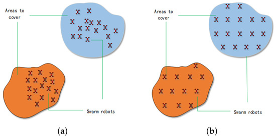
Figure 1.
Scenario of swarm robots performing coverage tasks. (a) The initial distribution of swarm robots. (b) The adjusted distribution of swarm robots.
Definition 1
(Swarm robotic system). A swarm robot system is a system consisting of n robots, which we define as , where denotes an individual robot. Each individual robot can be described by a six-tuple . Where x represents the position of the robot and where the robot is regarded as a point with no shape or size, so x represents the coordinates of the point where the robot α is currently located. v represents the velocity vector of the robot α. represents the expected distance of the DVF of the robot α, that is, the distance that the robot α expects the surrounding robots to maintain. represents the maximum perception distance of the robot α, which means the range of information collected by a single robot, including the distribution of the target area within the range and other robot information. is used to indicate whether the individual robot has reached a state of convergence. represents the DVF vector perceived by the robot α.
In order to study the problem of adaptive uniform coverage based on dynamic virtual forces, in a swarm robot system, we define the control commands for each robot as follows:
- A Robot should be able to perceive each other within a certain range.
- For the neighbor robots that can be perceived, the distance and orientation relative to itself can be obtained.
- Each robot should be able to perceive the state of the surrounding area within a certain range, that is, to be able to distinguish the difference of pixels in different areas.
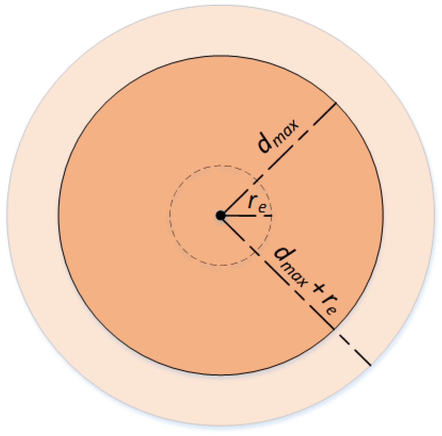
- Because robots are able to move, when the number of robots is not enough to cover the target area, the robots must be able to move themselves to patrol the surrounding areas, which means that the coverage area will be expanded to a certain extent. Assuming that the patrol radius of robot α is , the maximum coverage radius of robot α is , as shown in Figure 2. To further supplement Formula (1), for a certain pixel and a certain body robot α in the area, the definition of whether the pixel is covered by the individual robot α is updated to Formula (1).
 Figure 2. Robot coverage effect diagram under patrol.
Definition 2
(Cover state C). Let each robot be able to perceive the maximum distance (or the radius of the task that can be processed) as so the coverage area of the robot is . The environment is composed of a series of pixel point sets . For a certain pixel point and a certain body robot α, whether the pixel point is used by the individual robot α. The coverage is defined as Formula (2).
where is the distance from robot α to . If the position of the robot is then
Definition 3
(Coverage density T). The number of robots in the area D to cover is , so the number of robots per unit area in the area is the coverage density of the area, defined as Formula (3). In some practical applications, the number of robots required varies depending on the mission requirements, such as cleaning up oil pollution in the ocean, where areas with high levels of pollution require more robots. In this case, we divide the region into n sub-regions with densities of according to the demand, and high-density areas tend to require more robots.
Definition 4
(Four Neighbors N). The environment is a set composed of a series of continuous points, and each point can be described by a two-tuple . Among them, represent the coordinate position of in the two-dimensional plane space. Define each point in the area as the four-neighborhood N of this point, namely , where , that is, the four points at the top, bottom, left, and right positions of point .
Definition 5
(Area Boundary ). In the four-neighborhood of any point in the definition area, the set of points that do not belong to the area D can be judged as the area boundary, namely:
Problem 1.
With a given number of swarm robots, identify a method that enables the robots to complete coverage tasks in unknown areas in a self-organizing manner, while maintaining a certain distance between each robot.
Under the condition that all robots do not reach , that constant velocity is always maintained, and that the robots can move in any direction, the distance of the robot to complete the coverage task is one of the objects we need to optimize. The robots do not know the target area at first, which means that the shape of the target area is not clear, and there may even be obstacles in the area. In the deployment process, each robot can only perceive its local environment and formulate its own motion strategy according to its local interaction. In order to ensure that the swarm robots are as uniform as possible in the area, we must optimize the ideal distance between the robots.
For n robots, the optimization objective is determined according to Equations (5) and (6).
where M represents the total moving distance of the robot. and represent the positions of robot and robot respectively; d represents the ideal distance between robots, and represents the neighbor node set of robot .
Problem 2.
For sub-regions with different densities in the target area, a method that can deploy a corresponding number of robots in different densities areas is determined.
Areas with different densities have different priorities. Areas with higher densities have higher priorities, and more robots need to be deployed. For sub-regions with different densities with unknown shapes in the target area, deploying a corresponding number of robots is a difficult problem.
In this section, the formulas of the proposed method are related to the algorithms. We use three indicators to evaluate the performance of completing tasks: (1) the coverage rate based on robots’ final positions, (2) the uniformity based on the robots’ final positions, (3) the total distance the robots moved. Our ultimate goal is that the swarm robots will maximize the coverage area uniformly.
3.2. Adaptive Adjustment of Adjacent Distance
Assuming that the robots enter the designated area from any direction, the distribution of the robots after entering the designated area is not uniform at the beginning. For the uneven distribution of the robots, we can easily give an indicator of whether the area is uniform. The macroscopic non-uniformity for a single robot is the anisotropy of the number of surrounding robots, that is, if there are more robots in a certain direction, the robot should be far away from this direction, otherwise, the robot should be closer to this direction.
We propose a method of dynamic equalization of virtual force, which prompts the robot to move in the direction that will eliminate anisotropy. Assume that the set of robot within perceptible distance is . The distance between robot and a certain robot in the robot set is , and the average of the distance between and all the robots around it is defined as Formula (7).
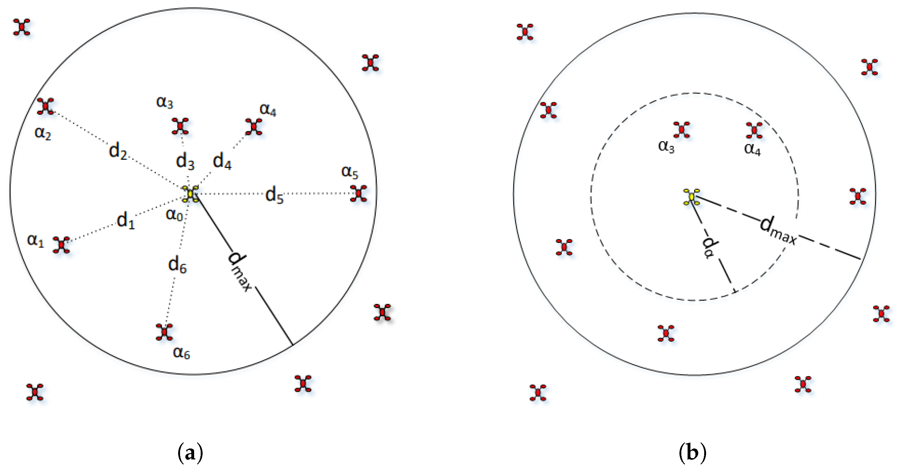
The distance relationships between each robot and its neighboring robots are shown in Figure 3. Intuitively, represents the minimum distance between and the surrounding robot , and it is also the DVF range of the individual robot. Let be the distances from to , it can be seen from Figure 3 that only two robots are in the range of , which means that only these two robots will produce a virtual repulsive force towards robot .
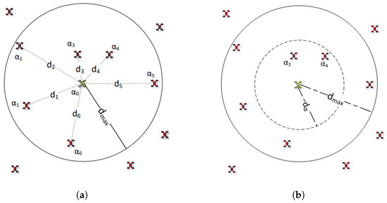
Figure 3.
The distance relationships between a robot and neighboring robots. (a) The distances between each robot and all surrounding robots. (b) The average distance between each robot and all surrounding robots.
3.3. Interaction Scheme of Swarm Robots Based on Virtual Force
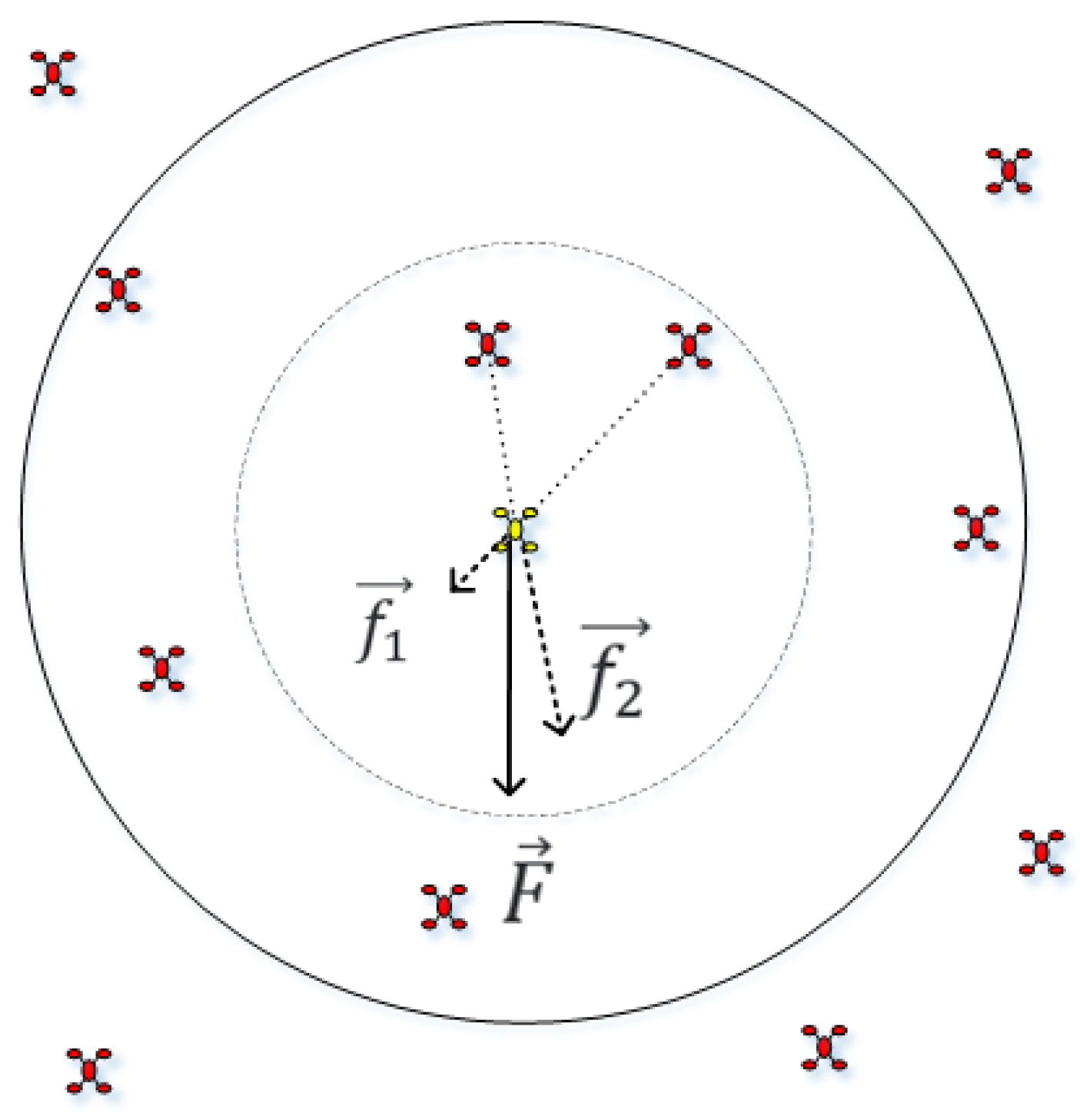
The resultant force generated by all the robots is to drive the robot to move, as shown in Figure 4.
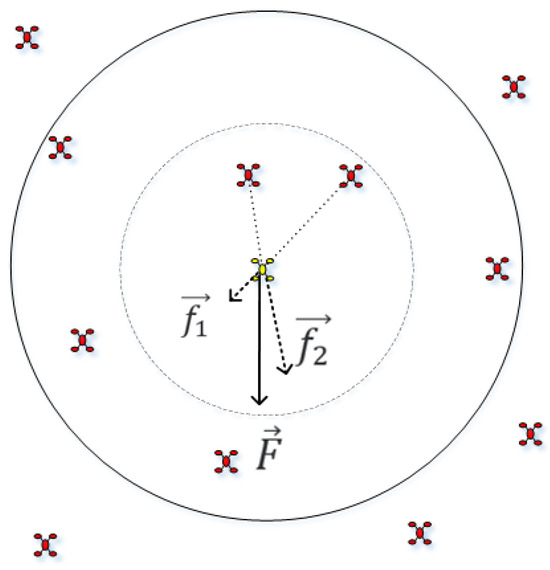
Figure 4.
Virtual force generated by surrounding robots.
Driven by the goal of expecting to maintain an average distance from all surrounding robots, once the distance between the robot around robot and is less than , a corresponding virtual repulsive force is generated by robot , and the vector means that means the force of on in the x-axis direction, and means the force of on in the y-axis direction. The specific calculation of the virtual force between robots is shown in Formula (8).
where is the angle between the vector from to and the positive half-axis of the x, and the direction of is from to ; and is average distance of robot ; and is a scaling coefficient that stabilizes boundary interactions by preventing excessive repulsive forces from expelling robot beyond the area boundary. Obviously, the closer the robots are, the greater the virtual repulsive force generated. When the distance of all other robots within the expected distance of robot is equal to , the virtual force received by robot is zero. Through this DVF, the distribution of the robot and the surrounding robots becomes uniform. In the entire swarm robot system, each robot adjusts the distance between neighbors adaptively under the action of the mechanism described, so all of the robots are evenly distributed. This design embodies two critical sensitivities:
- 1.
- Force Coefficient : Scales the repulsive force magnitude. Larger a (e.g., ) accelerates swarm dispersion but risks boundary overshoot, while smaller a (e.g., ) stabilizes motion at the cost of delayed convergence.
- 2.
- Distance Threshold : Defines the effective repulsion range. Increasing enhances collision avoidance in dynamic environments, whereas decreasing optimizes dense formations but risks local congestion.
Through this adaptive DVF mechanism, robots dynamically adjust spacing to achieve uniform distribution. The logarithmic force model ensures repulsive intensity grows exponentially as , balancing global coverage with local collision avoidance.
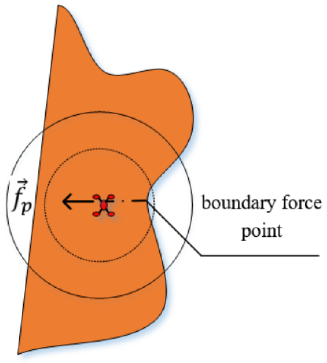
Additionally, when the robot is in the range where it can perceive the area’s boundary, several points can be extracted from the boundary of the area within the perceptive range of the robot, and a virtual repulsive force is generated for the approaching robot through these boundary points. The boundary of the area can restrain all the robots in its range. Each robot uses the closest point in its perception boundary to generate a boundary force point, and each boundary point can only act on the robot that is closest to it, as shown in Figure 5.
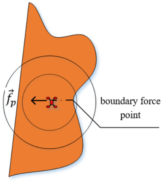
Figure 5.
Boundary points produce a virtual repulsion force on the robot.
The repulsive force generated by the boundary point p on the robot is calculated as shown in Formula (9).
where is the angle between the vector from p to and the positive half axis of the x-axis, the direction of is from p to , and a is a constant between 0 and 1. Therefore, the resultant force experienced by each robot is shown in Formula (10).
The calculation of the DVF directed towards by robot is shown in Algorithm 1.
First, the number of robots in the robot set around the robot is initialized and the average distance between the robot and the surrounding robots (lines 1–2), scan the swarm robots within the perception range of the individual robot, and update the values of and (lines 3–6). If the number of surrounding swarm robots is greater than or equal to 1, then update the dynamic virtual force range of the individual robot (lines 7–11). Then initialize the value of the virtual force and the resultant force (lines 12–13), scan the swarm robots in the dynamic virtual force range of the individual robot , and calculate the value of each swarm robot to the individual robot virtual force, and calculate the virtual force vector and (lines 14–17) generated by all the surrounding swarm robots, and scan the nearest boundary point in the dynamic virtual force range of the individual robot (lines 18–20). When there is a boundary point in the DVF range of the individual robot , calculate the virtual force of the boundary point for the individual robot , and update the virtual force resultant force (lines 21–22).
It is easy to calculate the total force direction of the robot through , so the position of the robot can be easily updated by using the kinetic formula, as shown in Formula (11).
where is the updated position of the robot after time t, and is the current position of the robot.
When the target area changes, the local area may increase or decrease. We adopt a random spreading mechanism for each boundary set point. Its four neighbors . Points in the target area all have a certain probability to randomly add to the target area, so as the area changes, the virtual forces on the robot will change accordingly and the robots in the whole area will be redistributed evenly.
| Algorithm 1: Dynamic virtual force update algorithm |
 |
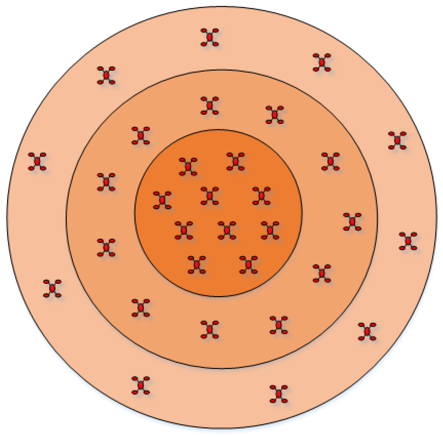
3.4. Adaptive Coverage Based on Different Densities
When swarm robots cover a task area, the number of robots needed at different locations in the area may be different, and we divide the area into multiple sub-regions with different densities according to the task requirements of the robots. High-density areas have higher priority than low-density areas, and high-density areas tend to require more robots to cover than low-density areas.
To assign the appropriate number of robots to sub-regions of different density, it is necessary to set different dynamic virtual forces for different priorities. Because the force between robots in different density areas is directional, the force is directed from the low density area to the high density area, so the swarm robots will also tend to gather in the high density area, as shown in Figure 6.
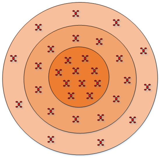
Figure 6.
Schematic diagram of density area division.
The virtual forces between robots in areas of different densities is , where is the density of the i-th area, and . Assume that the virtual force between robots in the first density area is , The virtual force between robots in adjacent density areas is the one of the previous density Times ( It is a constant set according to the needs of regional density), then the virtual force between robots in the i-th density area is:
3.5. Convergence Analysis
Even in a static environment, it is not possible to achieve convergence by stopping the robot by making the combined force . In fact, when a large number of robots are driven by DVFs to move, it is impossible to let the virtual force vector sum directed towards the robot remains at 0, and even the threshold that tends to 0 is difficult to set, which causes all robots to oscillate. In a dynamic environment, changes in the environment or changes in the number of robots are likely to cause frequent adjustments of the swarm robot system and cause oscillations. Therefore, it is necessary to set reasonable convergence conditions to determine the coverage of the robot population, so as to make the system relatively stable.
Since it is difficult for a single robot to judge the global coverage, it is necessary to convert the global convergence judgment into the convergence judgment of each robot. The robot records its own historical movement to determine whether it converged in the current position, based on the individual convergence probability to determine the global convergence of the entire swarm robot system.
Suppose that the latest q movement of robot is recorded as: , is the k-th movement of robot before . The historical displacement vector sum of the robot is shown in Formula (13).
Obviously, when the robot has not reached a relatively stable state, the historical movement will be in a certain general direction, and after reaching a relatively stable state, will oscillate without direction in a small range. Therefore, as the robot continues to reach a relatively stable state, will tend to decrease. The convergence threshold is set to , and when , the robot is in a stable state. If all robots in the swarm robot system meet the convergence state, the system is considered to be converged. The condition for system convergence is shown in Formula (14).
Therefore, the position update algorithm of the individual robot is obtained as shown in Algorithm 2.
When the movement of the individual robot does not converge, that is, the value of is false, the following loop is performed: first, set the value of the counter to a constant q, when each counter time is performed, the force on the individual robot is updated (line 2, call Algorithm 2), and move in the direction of the resultant force (lines 3–5), if the difference between the position of the individual robot and its historical position is less than the threshold , it is determined that the motion of the individual robot has converged, that is, (lines 6–8), and the information of the individual robot is updated (line 9). At the same time, the counter time is decreased by one unit (line 10).
| Algorithm 2: Individual robot location update algorithm |
 |
3.6. Algorithm Complexity Analysis
The algorithm’s complexity is analyzed from two dimensions: communication overhead and computational load.
- 1.
- Communication Overhead: Each robot communicates only with k neighbors within its perception range, achieving complexity (), which is significantly lower than the complexity of traditional methods.
- 2.
- Computational Load: Local force calculations and adaptive parameter updates for dynamic scenarios both incur complexity, independent of swarm size n.
3.7. Stability Analysis
In a swarm robot system, we wish to show that the swarm robot system can maintain stability during motion. Consider two neighboring points in the same direction, at time 0 and at time t. Let the spacing between these two points be and respectively, and let the number of robots be n. Then the Lyapunov exponent of the system in the same direction can be defined as:
Since the dynamic behavior of the robots in a swarm robotics system will gradually converge to a stable state and the value of the Lyapunov function will continue to decrease over time, thus indicating that the energy of the system is decaying at each time step. So when the exponent of the Lyapunov function is strictly less than zero, then the system is considered stable.
We substitute Formula (11) into the calculation and set the following initial parameters:
- is set to [−100, 100].
- Time t is set to 20,000.
Substituting gives , this shows that the swarm robot system in our proposed algorithm is stable.
4. Experiment and Analysis
To evaluate the effectiveness of the proposed method, we conducted a series of experiments. Simulation and experimental results verify the effectiveness of our proposed method. The experiment used the multi-agent simulation software NetLogo 6.4.0. The operating system was Win11(24H2), and the hardware resources included 16 GB memory and an i7 CPU.
The experimental conditions for all experiments in this section, as well as for the comparison experiments, are as follows:
- ①
- The speeds of the robots were the same.
- ②
- Each robot used its local coordinates to obtain the position of neighbor robots.
- ③
- The range of robot perception was limited.
- ④
- The initial position of each robot is randomly distributed.
- ⑤
- The task areas are all sized within 100 × 100 grid cells.
- ⑥
- For each method, 30 experiments were performed, and the analysis was performed by taking the average value.
The specific parameters were set as shown in Table 1. For the design of these parameters, whether the parameters are too large or too small will have a great impact on the experimental effect, for example, increasing the sensing distance can increase the interaction and coordination between the intelligences, but too large sensing distance will also increase the overhead accordingly. Therefore, we initially set random values, and then we design the three objective functions of maximizing the area coverage, the uniformity of area coverage, and the total distance moved by the robot, and continuously adjust the control parameters to achieve the optimal value of the objective function through multiple experiments and optimization.

Table 1.
Static single area robot adaptive coverage experiment parameters.
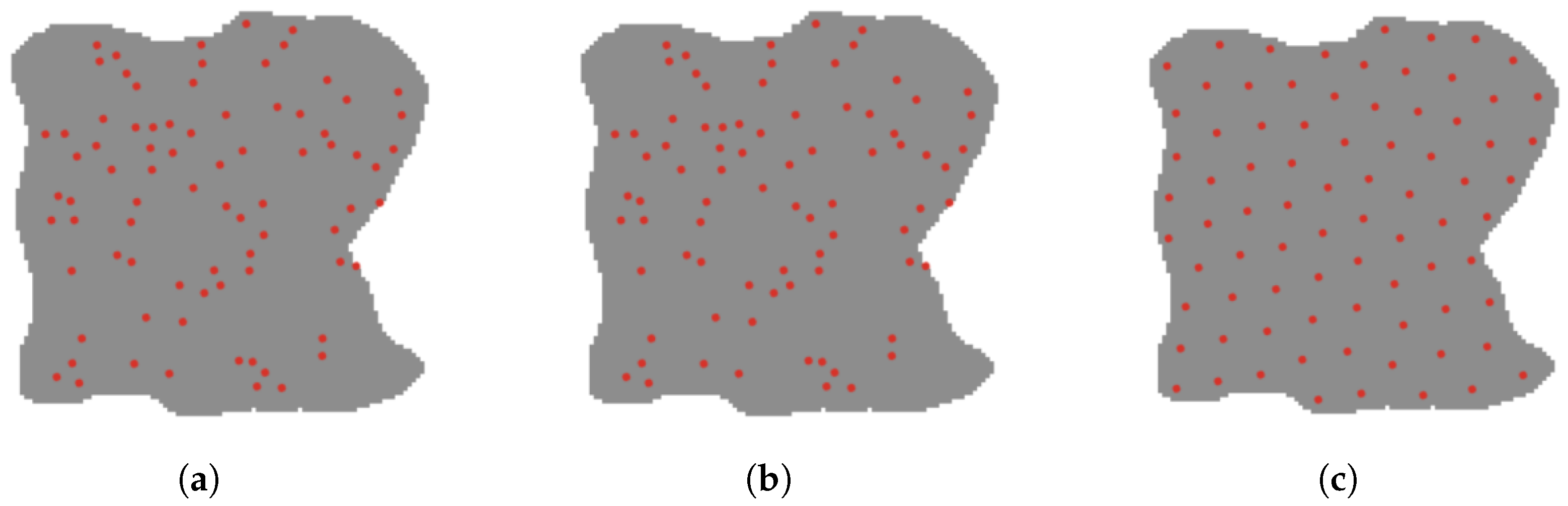
Aiming at a target area given a specific shape in a two-dimensional plane, we used 10–100 robots to conduct multiple adaptive coverage experiments on the target area. Figure 7 shows the process of achieving adaptive uniform coverage of the target area by 80 robots. At first, the robots are randomly distributed in the 2D environment outside the target area (Figure 7a). Then the robots enter the target area to cover (Figure 7b). Finally, the robot achieved uniform coverage of the target area through adaptive adjustment (Figure 7c).
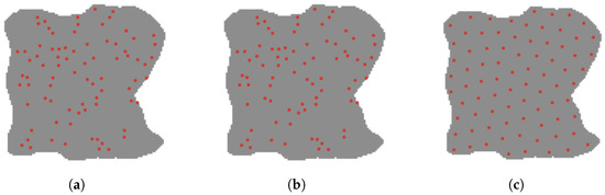
Figure 7.
Experimental diagram of adaptive uniform coverage based on dynamic virtual force. (a) Random distribution of robots. (b) Adaptive adjustment. (c) Robots’ adaptive, even coverage.
The swarm robots’ coverage rate and uniformity of coverage are analyzed separately. Different numbers of robots 10–100 were set to verify the robustness and scalability of the algorithm, and the coverage entropy is used to evaluate the coverage uniformity. We use the coverage entropy H to evaluate the swarm robots’ uniformity of coverage over the target area. Entropy can be used to express the uniformity of any kind of energy distribution in space. The more uniform the energy distribution, the greater the entropy. The size of the covering entropy H reflects the orderliness of the system, which is defined as Equation (16). It can be seen that when x obeys the uniform distribution, the corresponding entropy is the largest.
where is the ratio of the coverage area of individual robots to the coverage area of all robots, expressed as Formula (17).
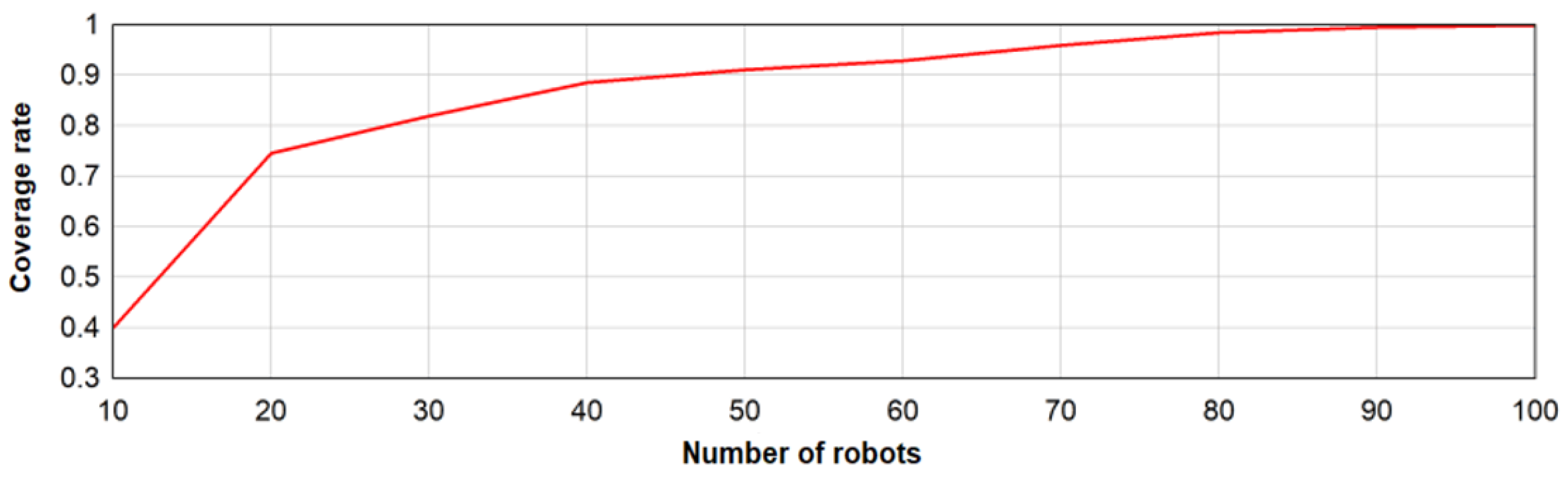
4.1. The Impact of the Number of Robots on Area Coverage
The area coverage statistics of different numbers of robots are shown in Figure 8. The coverage rate of robots to the same target area increases with an increase in the number of robots. When the number of robots exceeds 80 or more, the coverage rate of the target area can be close to 100%. Experiments show that the robots’ coverage rate is related to the number of robots. An increase in the number of robots increases the coverage rate linearly. When the number is small, the growth rate is faster. When the number exceeds 40, the growth rate gradually flattens out.
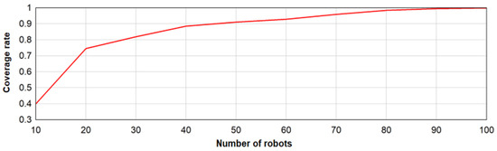
Figure 8.
Number of robots to area coverage.
4.2. Robot Coverage Uniformity Evaluation
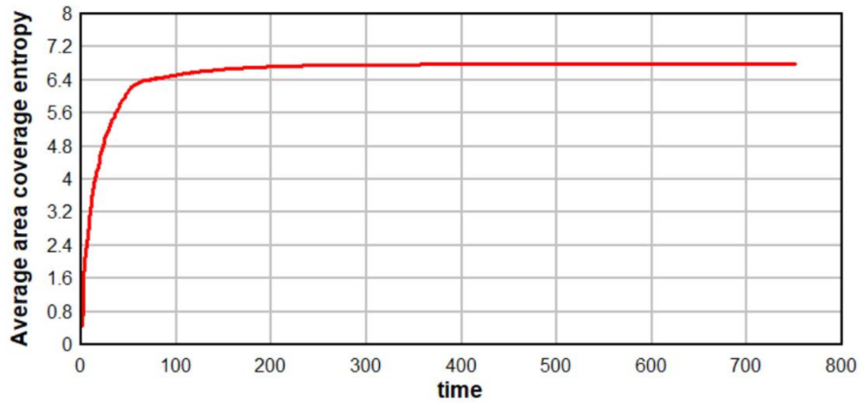
The average area coverage entropy of 80 robots is shown in Figure 9. The entropy’s size reflects the system’s orderliness, and the gradual decrease in coverage entropy from small to large reflects that the uniformity of the robots coverage is improving. After the system is stable, the coverage entropy no longer changes.
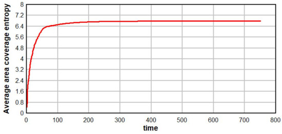
Figure 9.
Swarm robots’ average area coverage entropy.
4.3. Robot Coverage Stability Evaluation
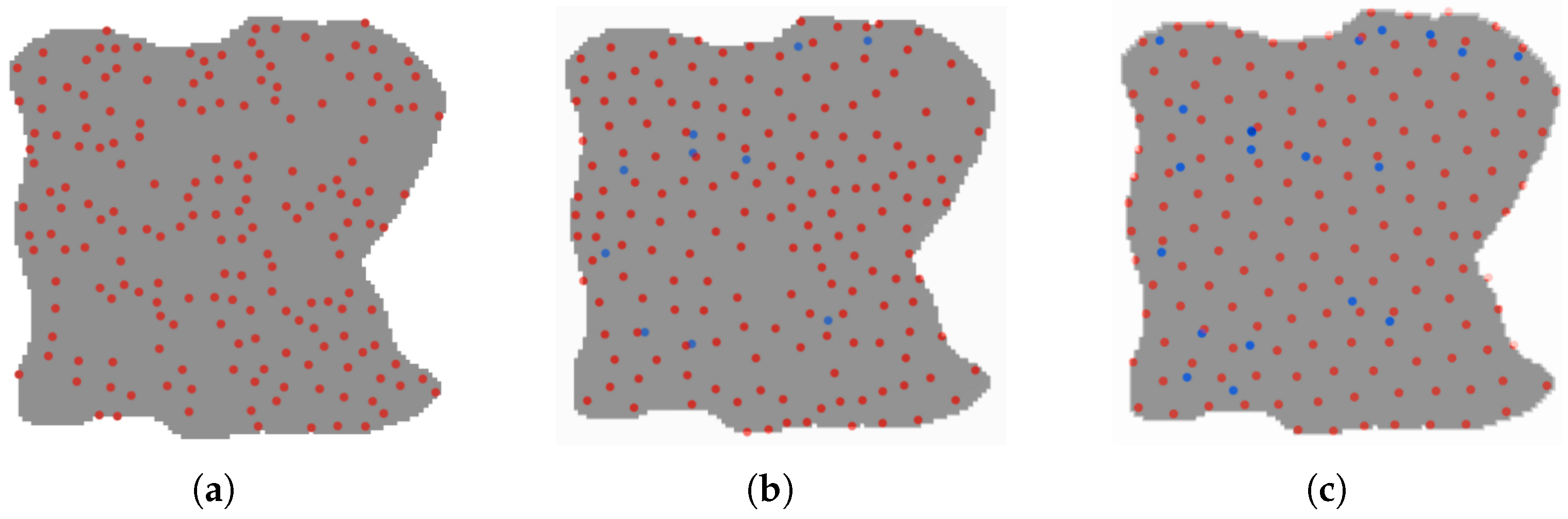
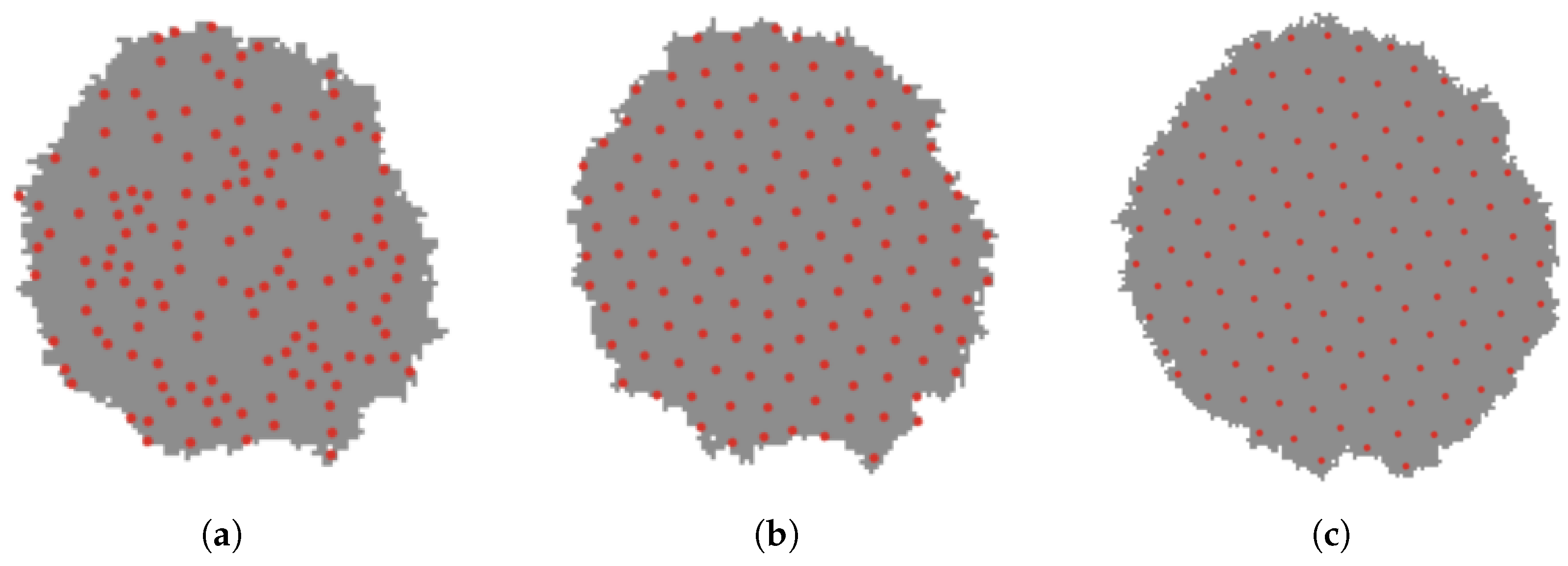
We designed a robot failure experiment in which the total number of robots in the simulation was set to 180, and the number of faulty robots gradually increased from 0 to 20 over time. The experimental process is illustrated in Figure 10. The results demonstrate that under the DVF method, the remaining non-faulty robots can still accomplish the uniform coverage task, validating the algorithm’s exceptional robustness.
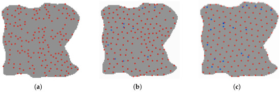
Figure 10.
Experimental diagram of adaptive stability coverage based on dynamic virtual force. (a) Initial position. (b) Adaptive adjustment. (c) Final position.
4.4. Coverage Experiment with Different Area Shapes and Obstacles
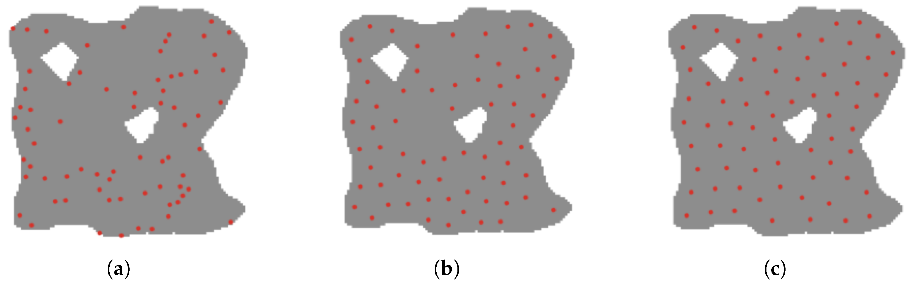
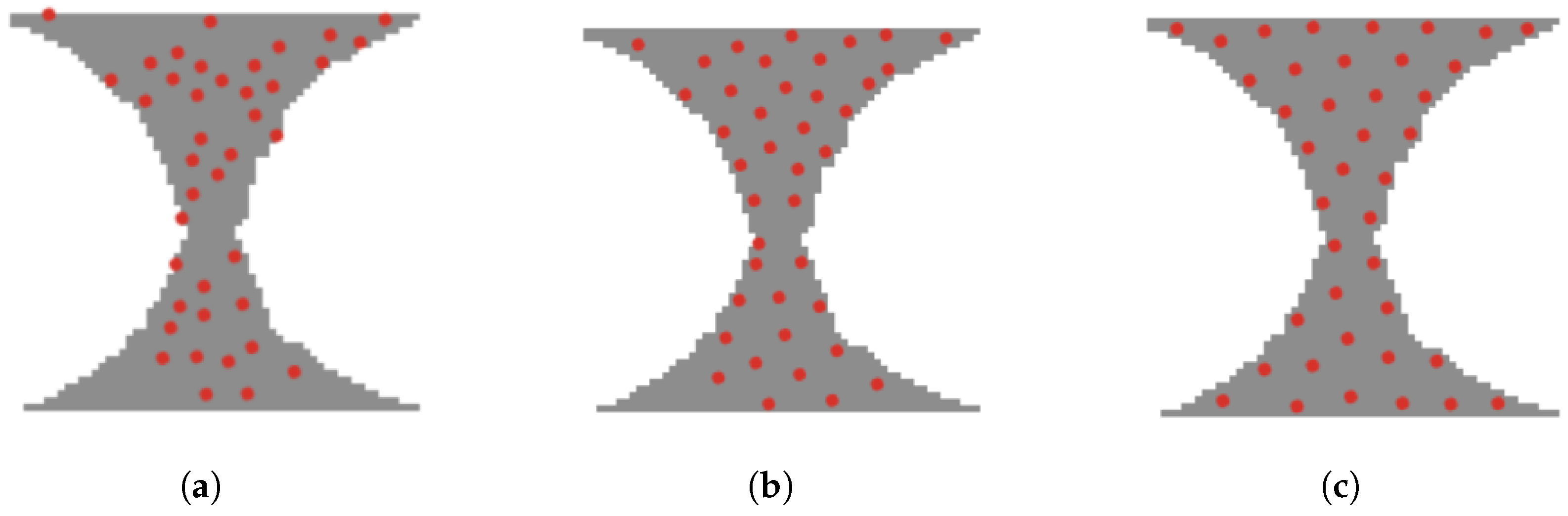
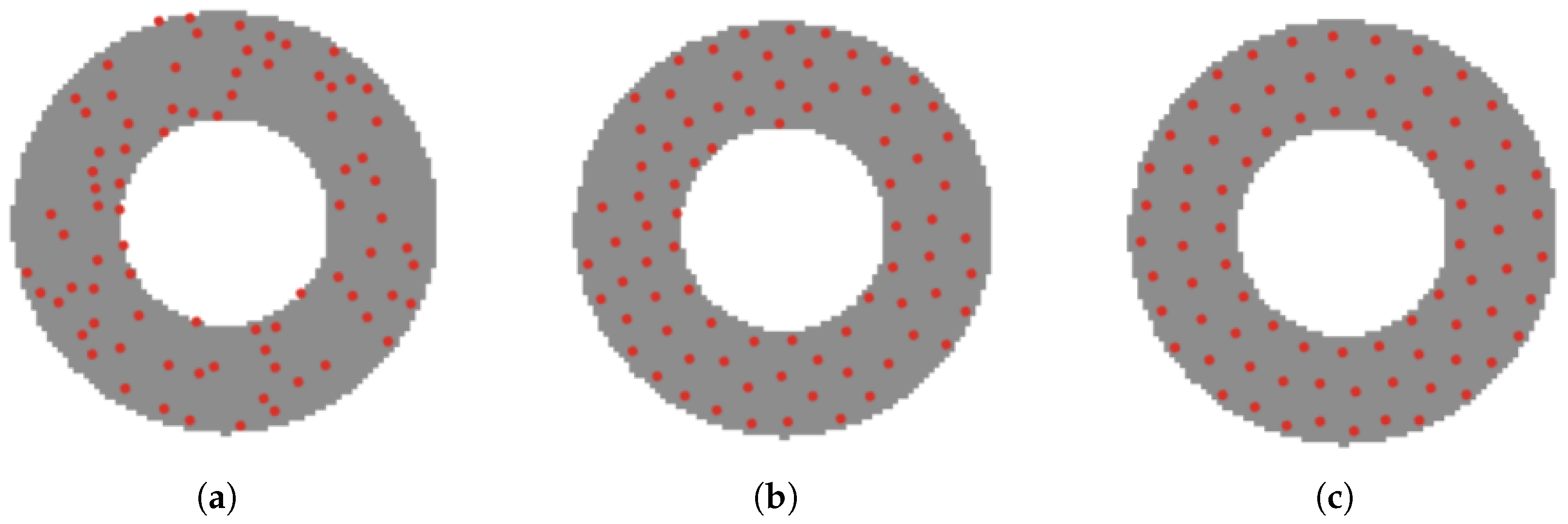
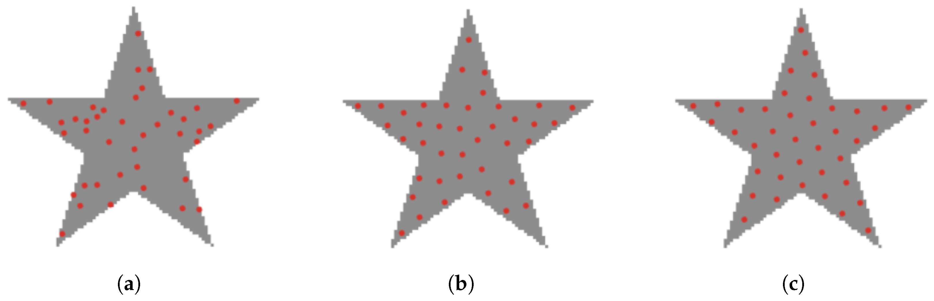
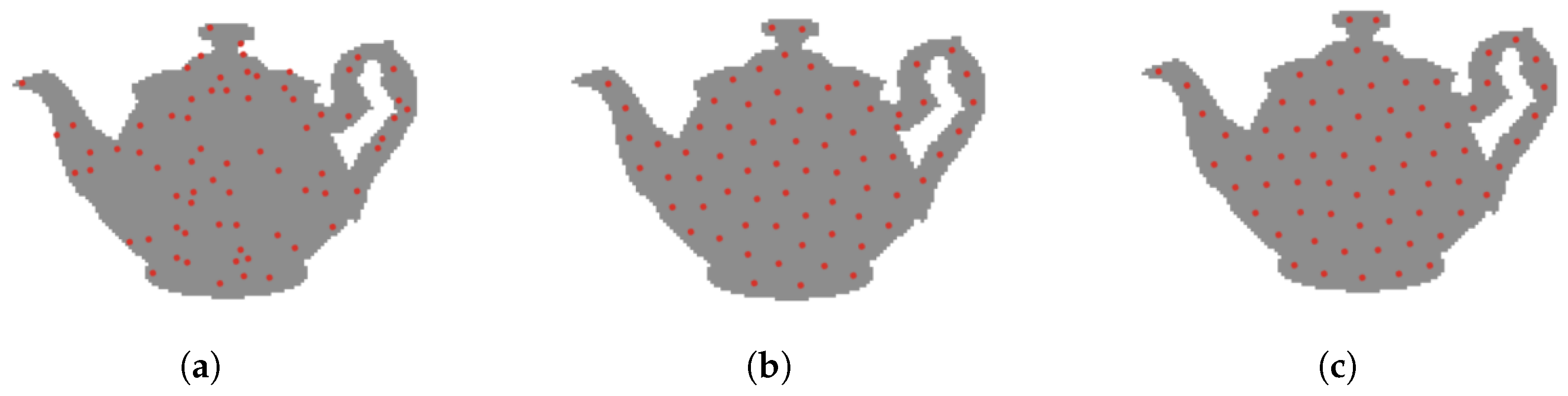
We conducted experiments on areas with different shapes and obstacles, as shown in the Figure 11, Figure 12, Figure 13, Figure 14 and Figure 15, and selected three phases of the experiment and each phase was spaced 5 s apart: an initial random distribution phase, an adaptive adjustment phase, and a final completion phase with uniform coverage. We used 10–100 robots to carry out adaptive coverage experiments on areas with different shapes and obstacles in the area for many times. Figure 11 shows the adaptive and uniform coverage process of 70 robots when there were two obstacles (white holes) in the area. It can be seen that the robot still maintains a uniform coverage in the environment with obstacles. Figure 12 shows the process of adaptive uniform coverage by 40 robots in a funnel-shaped region. The figure takes into account the presence of edges, corners and narrow channels in the region, and the robots can move to the optimal coverage position. Figure 13 shows the process of adaptive uniform coverage of 70 robots in the case of an annular region shape, and they still move adaptively to uniform coverage. Figure 14 shows the process of adaptive uniform coverage of 80 robots in an area with the shape of the letter ‘K’, it’s easy to find that the target areas are covered adaptively in an area with curves and corners. Figure 15 shows the process of adaptive uniform coverage of 40 robots in the shape of a five-pointed star, and Figure 16 shows the process of adaptive uniform coverage of 70 robots in the shape of a teapot. It can be seen that the robots maintain uniform coverage in the case of regions with different shapes and obstacles in the region.
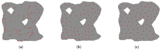
Figure 11.
Two obstruction conditions in the area. (a) Initial position. (b) Adaptive adjustment. (c) Final position.
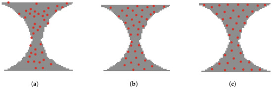
Figure 12.
Area is funnel-shaped. (a) Initial position. (b) Adaptive adjustment. (c) Final position.
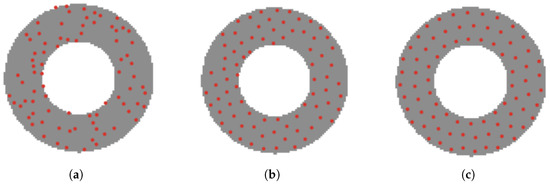
Figure 13.
Area is circular. (a) Initial position. (b) Adaptive adjustment. (c) Final position.
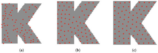
Figure 14.
Area is the letter ‘K’. (a) Initial position. (b) Adaptive adjustment. (c) Final position.
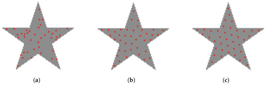
Figure 15.
Area is a five-pointed star. (a) Initial position. (b) Adaptive adjustment. (c) Final position.
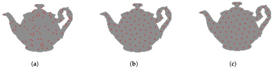
Figure 16.
Area is the shape of teapot. (a) Initial position. (b) Adaptive adjustment. (c) Final position.
4.5. Coverage Experiment of Regional Dynamic Change
The dynamic area adaptive coverage algorithm effectively enables uniform coverage of dynamic regions. In the dynamic environment experiment, the number of robots was set to a fixed value, and the coverage area dynamically expanded over time. The experimental process is illustrated in Figure 17. Experiments demonstrate that after swarm robots self-organize and enter a dynamic region with expanding area, the inter-robot distance increases proportionally to the region’s expansion, while they consistently maintain uniform area coverage.
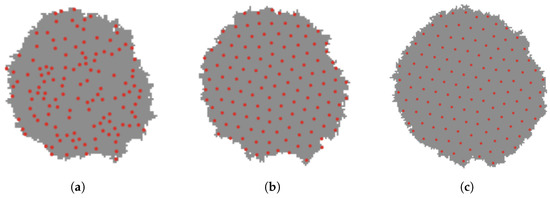
Figure 17.
Demonstration of dynamic area adaptive coverage process. (a) Initial dynamic area coverage. (b) Dynamic area coverage. (c) Dynamic area adaptive adjustment.
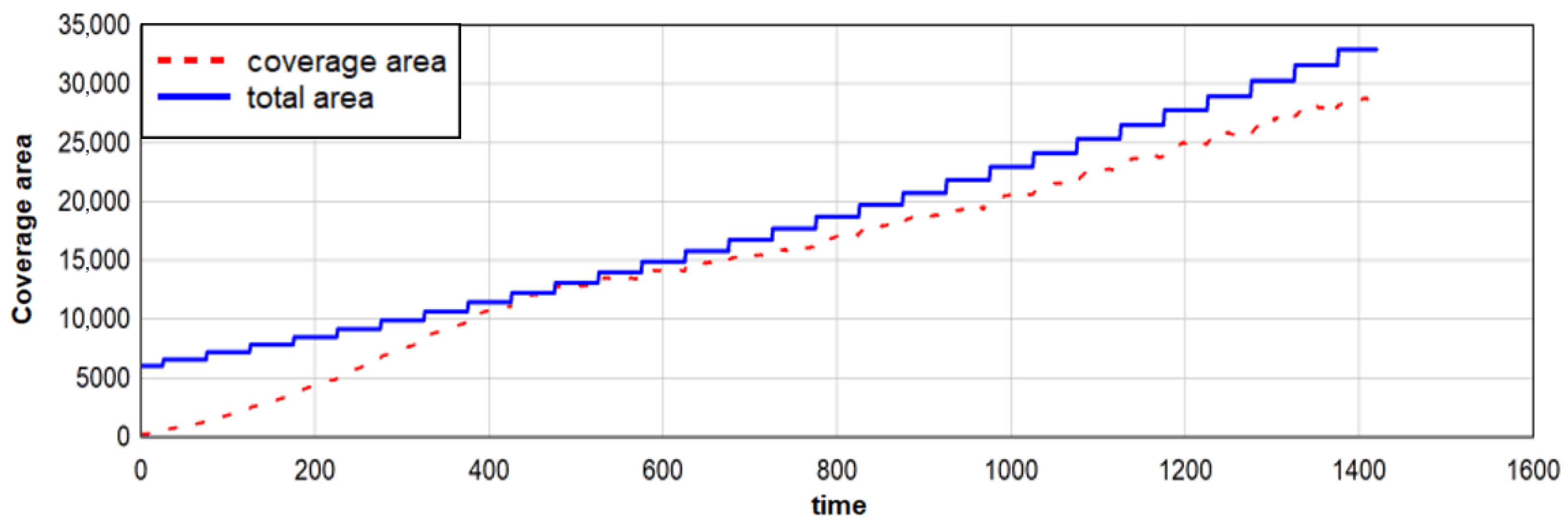
In the case of a dynamic region, we measured the total area change and the coverage area change curve, as shown in Figure 18. In the experiment, there were 130 robots, and area is expanded at 50 time units intervals.
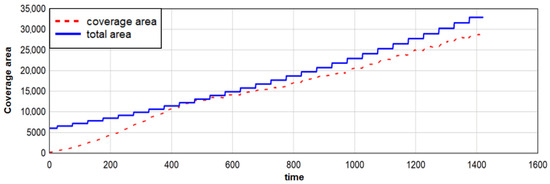
Figure 18.
Change process of dynamic area coverage.
Figure 18 shows that when the robot was first covered, the coverage area continued to rise until it was close to the total area of the area. In the subsequent regional spreading process, the robots could quickly reach convergence, and the coverage area expanded with the expansion of the area’s size.
4.6. Coverage Experiment Based on Different Densities Areas
The schematic diagram of coverage experiments based on different densities areas reveals in Figure 19. Figure 19a shows the process of adaptive uniform coverage by 70 robots in the five-pointed star area. Figure 19b shows the process of adaptive uniform coverage by 130 robots in the letter ‘K’ area. Figure 19c shows the process of adaptive uniform coverage by 140 robots in the multi-layer ring area.The figures show different densities in different colors. The higher the density, the higher the priority of the area, so more robots are deployed to the area, and the robots have a higher coverage density. The smaller the density, the lower the priority of this area, so fewer robots are deployed, and the robots have a smaller coverage density. In the same priority area, the robot can still maintain uniform coverage.
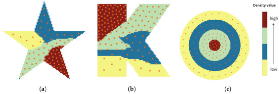
Figure 19.
Schematic diagram of multi-densities adaptive coverage. (a) Area is five-pointed star. (b) Area is the letter ‘K’. (c) Area is the multi-layer ring.
4.7. Benchmark Problem Design
We defined 20 benchmark problems for the area coverage problem, which are summarized in Table 2. Seven maps are used in the benchmark problem, taking into account various variations in map characteristics, including differences in map shape, dynamic changes in map area, density divisions in the map, and the presence of obstacles in the map. Table 3 shows the performance of DVF in terms of several performance indices: the coverage rate and the statistical confidence and standard deviation of coverage, the coverage uniformity, the distance of movement, and the time required for convergence. From the table, we can see that in the same map, the more the number of robots, the larger the coverage rate of the area, and the larger the total distance moved, but the entropy is getting smaller, such as No. 2 and No. 4 in the table, although the coverage rate of No. 4 is larger than that of No. 2, when the number of robots is increased, the coverage of multiple robots overlap, which results in the coverage uniformity of a swarm robot system decreases. However, this is not certain, for example, No. 18 has more robots than No. 17, and the entropy value is also larger than it, so the map shape has some influence on the change of entropy value.
Table 2.
Benchmark problem configurations.
Table 3.
Experimental results.
4.8. Performance Verification Experiment in a Noisy Environment
To verify the stability of the DVF algorithm under noise interference, three benchmark problems (No. 3, No. 5, and No. 20) in Table 2 were selected as representatives of coverage problems in static areas, dynamic areas, and multi-density areas, respectively. Experiments and analyses were conducted in these different environments to validate the robustness of the DVF algorithm. The noise settings are shown in Table 4.
Table 4.
Noise type description.
The experiment was repeated 30 times and the average value was taken, the key indicators being the coverage rate, the uniformity of coverage and the distance of movement. The simulation results for No. 3 are shown in Table 5. The simulation results for No. 5 are shown in Table 6. The simulation results for No. 20 are shown in Table 7.
Table 5.
Experimental results for No. 3.
Table 6.
Experimental results for No. 5.
Table 7.
Experimental results for No. 20.
The experimental results show that as the noise intensity increases, both the coverage rate and the coverage entropy decrease accordingly, while the total moving distance increases, but the overall trend of degradation of the performance is mild. Mixed noise has the greatest impact on the algorithm, yet a relatively high coverage level is still maintained. Due to the complexity of the scenarios, the performance degradation caused by noise in the dynamic star area (No. 5) and multi-density star area (No. 20) is slightly greater than that in the static star area (No. 3), but the gap is controlled within 2%. In summary, the stable performance of the DVF algorithm under the combination of various noise interferences and complex scenarios confirms that the algorithm has good robustness.
4.9. Comparison of Different Coverage Methods
In the context of the environment introduced at the beginning of Section 4, the DVF method proposed in this paper is compared with four area coverage algorithms that use different approaches, including VFA algorithm [27], OAVFA algorithm [28], K-means-DCC algorithm [43], and BAPS algorithm [36]. For comparison, the main performance comparisons include coverage rate, total robot movement distance, coverage uniformity (coverage entropy) and time required for convergence.
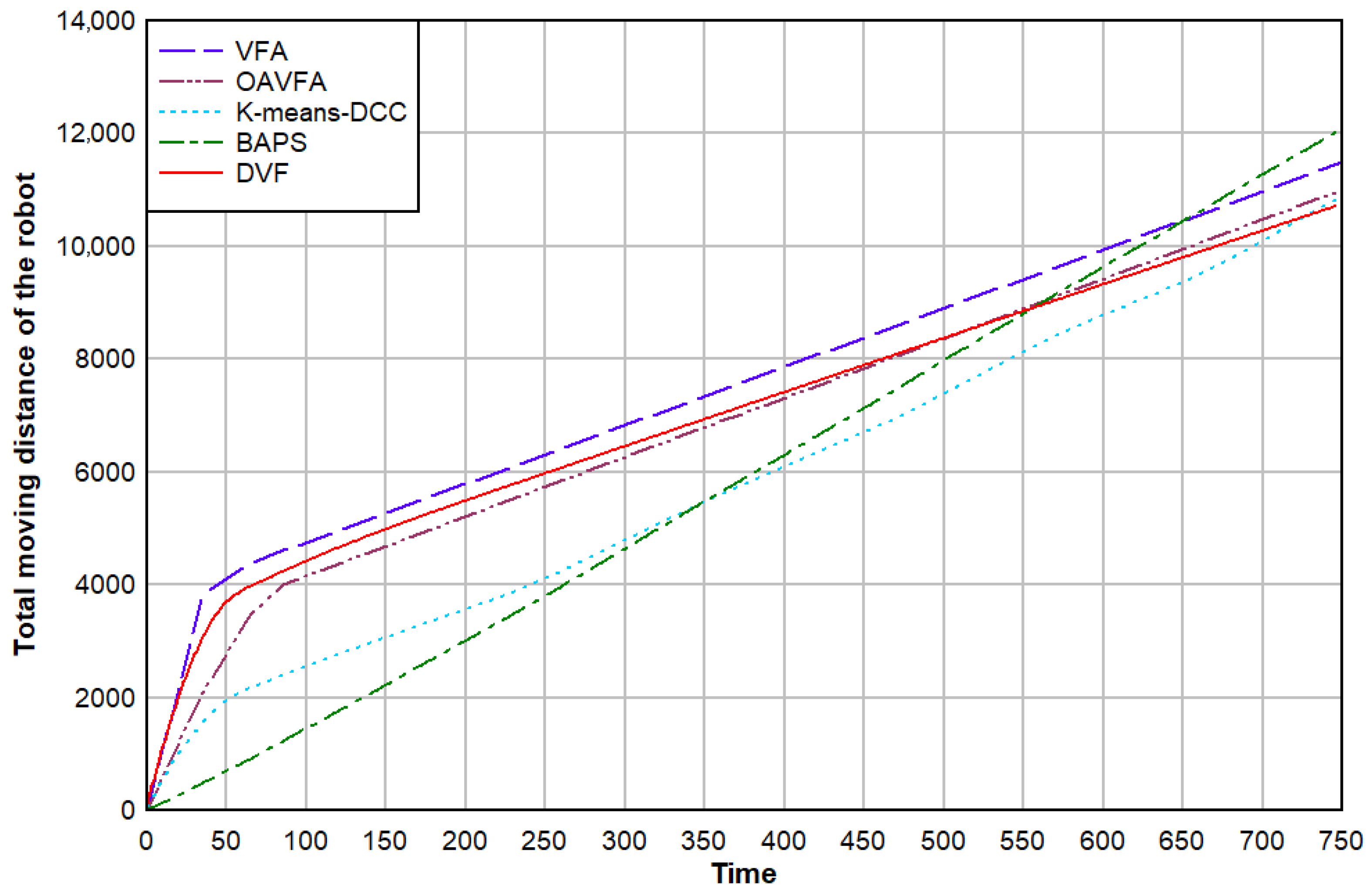
4.9.1. Total Distance of Robot Movement
Figure 20 shows the total distance that the group of robots moved in the area coverage experiment with each. The moving space of the robot in the K-means-DCC method is smaller than that in the BAPS method. In our DVF method, because the robots repel each other, the robots will be quickly scattered in the initial period, so the distance moved at the beginning is the largest, after a certain period, the growth rate of the total moving distance of the robot is lower than that of the K-means-DCC method and the BAPS method.
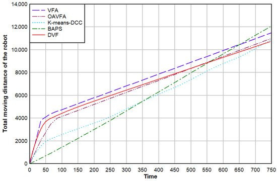
Figure 20.
Comparison of the total moving distance of the robot.
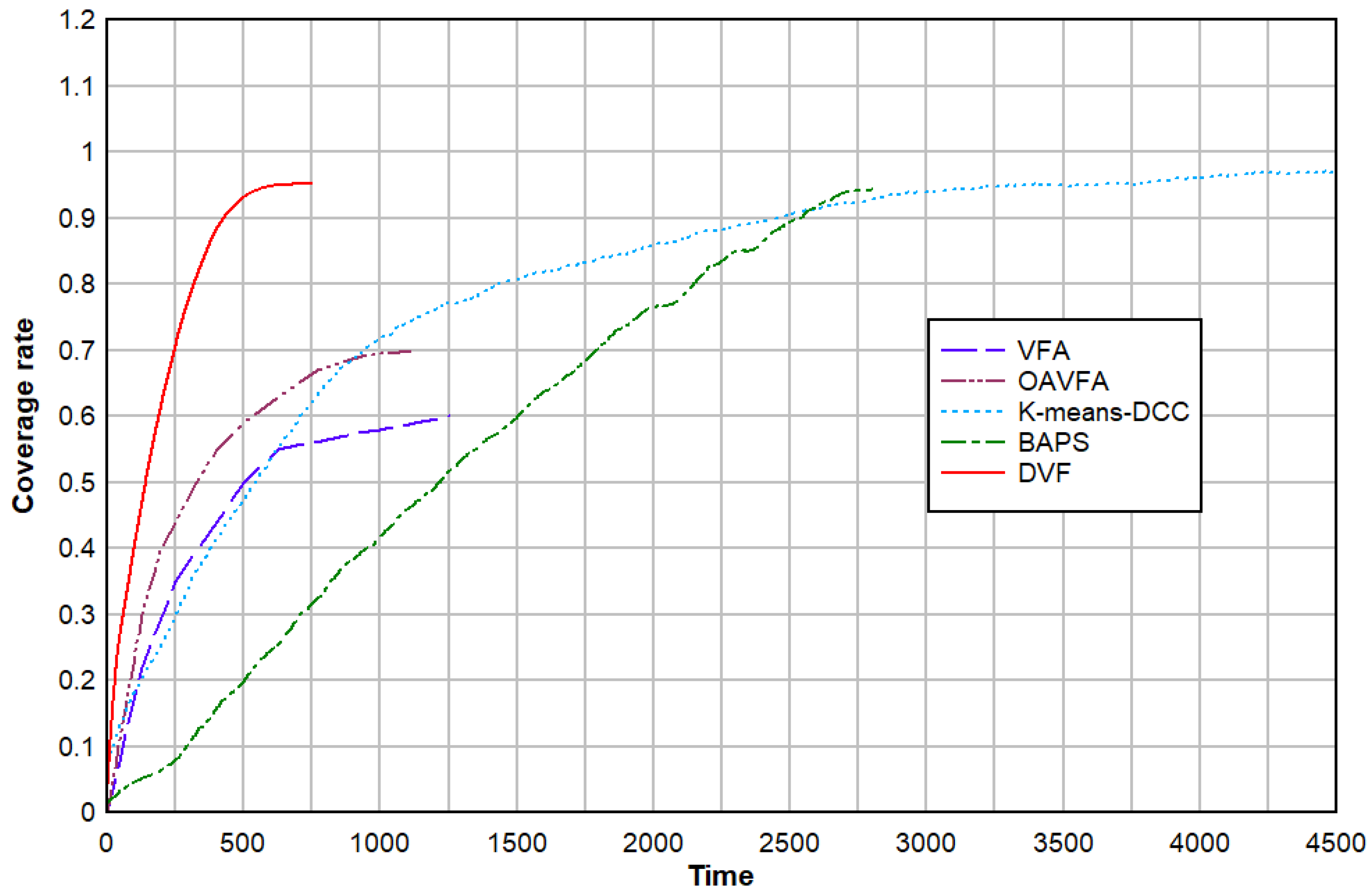
4.9.2. Coverage Rate
Figure 21 shows the coverage changes for each method in the area coverage experiment. Due to the limited number of robots, the coverage rate of the angle-first approach that uses the proximity of the robots is meager. Although the K-means-DCC method has a high coverage rate, the method must determine the distance between the robots before the coverage, and then it cannot be dynamically adjusted. The BAPS method can dynamically adjust the distance between robots, but the coverage is relatively slow. In contrast, the DVF method can quickly and dynamically adjust the distance between robots, allowing a limited number of swarm robots to promptly complete the area coverage, with a coverage rate of over 98%.
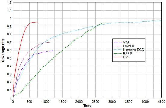
Figure 21.
Comparison of regional coverage rate.
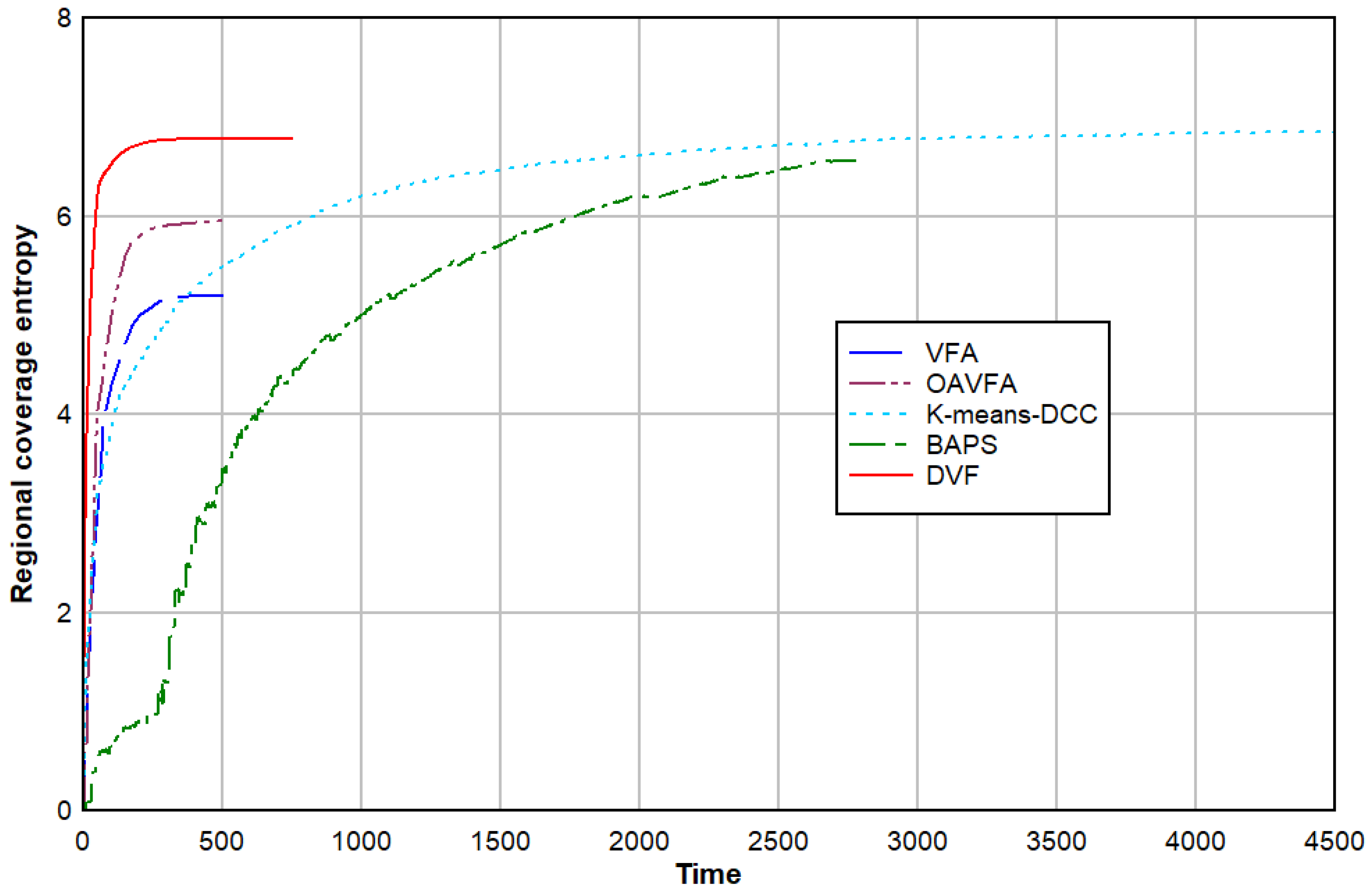
4.9.3. Coverage Uniformity
The uniformity of area coverage can be evaluated by defining the area coverage entropy, which reflects whether the distance between all robots in the swarm robot system covering the area is consistent. Figure 22 shows the four methods can achieve uniform coverage. Still, the DVF method can achieve uniform coverage quickly, and the coverage entropy is the largest; the K-means-DCC method is the second largest, and the BAPS method is the slowest.
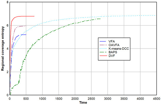
Figure 22.
Comparison of regional coverage entropy.
4.9.4. Other Comparative Experiments
To verify the effectiveness of our algorithms in improving coverage performance, we will do experiments and analysis of these four comparison algorithms in different environments based on the benchmark problems No. 1, No. 2, No. 4, No. 5, No. 6, No. 19. Except for No. 1 which is a circular map, the other five problems are implemented on a star-shaped map to be able to better compare the effect of the algorithm in different scenarios under the same map. The simulation results are presented in Table 8.
Table 8.
Results of comparative experiments.
As Problem No. 1 in Table 8, in a simple circular map, the results for coverage and total distance traveled are very similar for the five algorithms, but the DVF algorithm works better for coverage uniformity and convergence time. For Problem No. 2, when corners appear at the boundaries of the region, the VFA algorithm has a worse coverage effect than the other four algorithms. For Problem No. 4, we observe that as the number of robots increases, the coverage rate of each algorithm becomes better, but the coverage uniformity is relatively worse. For Problem No. 5, when there is a dynamic change in the environment of the map, only the DVF algorithm still has a good coverage; none of the other algorithms gives as good results as in the static environment. For Problem No. 6, each algorithm takes into account the presence of obstacles in the map, but only the DVF algorithm performs best in terms of uniformity of coverage, especially the ability to cover the task with minimum movement distance. For Problem No. 19, when the map contains sub-regions requiring different numbers of robots, other algorithms exhibit poor coverage, whereas the DVF algorithm maintains both a high coverage rate and uniformity. Additionally, across six problem instances, the DVF algorithm’s convergence time significantly outperforms that of other methods, an advantage stemming from its distributed computing architecture. This demonstrates the algorithm’s effective adaptation to diverse environments.
4.9.5. Conclusions
Finally, Table 9 compares various methods of swarm robots’ area coverage, the experimental setting is the same as at the beginning of Section 4. We can find that for these area coverage algorithms, large-scale areas and complex areas are considered. Still, most algorithms do not consider regional changes or the existence of sub-areas with different densities in the region. The algorithm proposed in this paper can perform well in various conditions, and the coverage rate and speed are better than most of the algorithms we compared it to.
Table 9.
Comparison of various methods of swarm robots’ area coverage.
5. Conclusions and Future Works
This article focuses on improving the ability of swarm robots to cover an area uniformly and completely. A DVF adaptive area coverage method is proposed, which is suitable for monitoring dynamic environments. Our method only needs to focus on the robot and its neighboring parts of the robot, without the need for global information transfer, which is a distributed feature that can reduce the communication overhead and is more easily scalable to large-scale systems. And our method has fewer parameters and focuses mainly on the calculation and tuning of the repulsive force. This makes it relatively easy to adjust the parameters of the algorithm and reduces the complexity of parameter optimization. In our experiments, it does not fall into local optimal solutions in areas of complex shapes and still performs well. The coverage rate, coverage speed, and coverage uniformity in the self-organizing algorithm are better than most existing algorithms, and the effectiveness of the method is ensured by experiments. In addition, the DVF method was used to achieve different coverage densities for to cover areas that varied in their importance, which can be successfully applied to practical tasks such as cleaning up marine crude oil leakage. In the future, our future research will focus on two core directions. First, we will deploy the DVF algorithm proposed in this paper onto real robotic platforms for systematic performance testing. By constructing a physical experimental environment with complex terrains and dynamic obstacles, we aim to validate the algorithm’s actual coverage efficiency, motion stability, and fault tolerance in the physical world. Second, we will introduce multi-dimensional noise interference during testing, including sensor ranging errors, communication link packet loss, and actuator delays to more closely mimic real-world application scenarios. Based on the result of physical experiments, we will further optimize our algorithm.
Author Contributions
Writing—original draft preparation, W.Y.; Conceptualization, Methodology, M.K.; Data curation, Validation, Writing—Review and Editing, W.Y. Validation and Formal analysis, Q.W. and Y.Z. All authors have read and agreed to the published version of the manuscript.
Funding
This work was supported in part by the National Natural Science Foundation of China (Grant No. 32430062), in part by the Doctoral Research Start-up Project (Grant No. 22QDZ03), in part by the Natural Science Foundation of Hunan Province (Grant No. 2024JJ7543), in part by the China Higher Education Institution Industry-University-Research Innovation Fund (Grant No. 2024XL007), in part by the Hunan Provincial Social Science Fund (Grant No. 24JD073).
Data Availability Statement
The original contributions presented in this study are included in the article. Further inquiries can be directed to the corresponding author.
Conflicts of Interest
The authors declare no conflicts of interest.
References
- Alqudsi, Y.; Makaraci, M. Exploring advancements and emerging trends in robotic swarm coordination and control of swarm flying robots: A review. Proc. Inst. Mech. Eng. Part C J. Mech. Eng. Sci. 2025, 239, 180–204. [Google Scholar] [CrossRef]
- Zhu, P.; Song, R.; Zhang, J.; Xu, Z.; Gou, Y.; Sun, Z.; Shao, Q. Multiple UAV Swarms Collaborative Firefighting Strategy Considering Forest Fire Spread and Resource Constraints. Drones 2025, 9, 17. [Google Scholar] [CrossRef]
- Yan, X.; Chen, R. Application strategy of unmanned aerial vehicle swarms in forest fire detection based on the fusion of particle swarm optimization and artificial bee colony algorithm. Appl. Sci. 2024, 14, 4937. [Google Scholar] [CrossRef]
- John, J.; Harikumar, K.; Senthilnath, J.; Sundaram, S. An efficient approach with dynamic multiswarm of UAVs for forest firefighting. IEEE Trans. Syst. Man Cybern. Syst. 2024, 54, 2860–2871. [Google Scholar] [CrossRef]
- Srinivasan, A.; Babu, V.J. Review of Applications of Artificial Intelligence and Drones in Oil Pollution in Seawater. J. Comput. Commun. 2025, 13, 17–34. [Google Scholar] [CrossRef]
- Sajid, H.; Mubeen, M.; Al Zarooni, S.; Maheshwari, V.K.; Jaradat, M.A.; Khalil, A. Oil Spill Detection using Deep Neural Networks for Cleaning Robot Applications. In Proceedings of the 2024 Advances in Science and Engineering Technology International Conferences (ASET), Abu Dhabi, United Arab Emirates, 3–5 June 2024; pp. 1–6. [Google Scholar]
- Ardiny, H.; Beigzadeh, A. A study on the use of swarm robotics for environmental monitoring, radiation mapping and the discovery of radioactive sources. J. Nucl. Sci. Eng. Technol. (JONSAT) 2025, 46, 136–147. [Google Scholar]
- Khaldi, B.; Harrou, F.; Sun, Y. Collaborative Swarm Robotics for Sustainable Environment Monitoring and Exploration: Emerging Trends and Research Progress. Energy Nexus 2025, 17, 100365. [Google Scholar] [CrossRef]
- Abuali, T.M.; Ahmed, A.A. Innovative Applications of Swarm Drones in Disaster Management and Rescue Operations. Open Eur. J. Eng. Sci. Res. (OEJESR) 2025, 1, 23–31. [Google Scholar]
- Moosavi, S.K.R.; Zafar, M.H.; Sanfilippo, F. Collaborative robots (cobots) for disaster risk resilience: A framework for swarm of snake robots in delivering first aid in emergency situations. Front. Robot. AI 2024, 11, 1362294. [Google Scholar] [CrossRef]
- Das, S. Harvesting Tomorrow: Transformative Applications of Swarm Robotics in Agriculture. In Bio-Inspired Swarm Robotics and Control: Algorithms, Mechanisms, and Strategies; IGI Global: Hershey, PA, USA, 2024; pp. 193–210. [Google Scholar]
- Abhang, L.; Gummadi, A.; Changala, R.; Vuyyuru, V.A.; Raj, I.I. Swarm Intelligence for Multi-Robot Coordination in Agricultural Automation. In Proceedings of the 2024 10th International Conference on Advanced Computing and Communication Systems (ICACCS), Coimbatore, India, 14–15 March 2024; Volume 1, pp. 455–460. [Google Scholar]
- Zhang, S.; Huang, Y.; Li, W.; Pan, J. Swarm Robotic Flocking with Aggregation Ability Privacy. IEEE Trans. Autom. Sci. Eng. 2025, 22, 10596–10608. [Google Scholar] [CrossRef]
- Nguyen, L.V. Swarm Intelligence-Based Multi-Robotics: A Comprehensive Review. AppliedMath 2024, 4, 1192–1210. [Google Scholar] [CrossRef]
- Devi, K.V.R.; Smitha, B.; Lakhanpal, S.; Kalra, R.; Sethi, V.A.; Thajil, S.K. A review: Swarm robotics: Cooperative control in multi-agent systems. E3S Web Conf. 2024, 505, 03013. [Google Scholar] [CrossRef]
- Cheng, B.; He, M.; Zhu, Z.; He, B.; Chen, J. Development and Application of Coverage Control Algorithms: A Concise Review. IEEE Trans. Autom. Sci. Eng. 2025, 22, 14906–14927. [Google Scholar] [CrossRef]
- Palacios-Gasós, J.M.; Montijano, E.; Sagues, C.; Llorente, S. Multi-robot persistent coverage using branch and bound. In Proceedings of the 2016 American Control Conference (ACC), Boston, MA, USA, 6–8 July 2016; pp. 5697–5702. [Google Scholar]
- Sun, X.; Ren, M.; Ding, D.W.; Cassandras, C.G. Optimal coverage control of stationary and moving agents under effective coverage constraints. Automatica 2023, 157, 111236. [Google Scholar] [CrossRef]
- Jayalakshmi, K.; Nair, V.G.; Sathish, D. A Comprehensive Survey on Coverage Path Planning for Mobile Robots in Dynamic Environments. IEEE Access 2025, 13, 60158–60185. [Google Scholar] [CrossRef]
- Atman, M.W.S.; Fikri, M.R.; Priandana, K.; Gusrialdi, A. A two-layer control framework for persistent monitoring of a large area with a robotic sensor network. IEEE Access 2024, 12, 4153–4165. [Google Scholar] [CrossRef]
- Alqudsi, Y.; Makaraci, M. Swarm robotics for autonomous aerial robots: Features, algorithms, control techniques, and challenges. In Proceedings of the 2024 4th International Conference on Emerging Smart Technologies and Applications (eSmarTA), Sana’a, Yemen, 6–7 August 2024; pp. 1–9. [Google Scholar]
- Alahmadi, A.; Barri, A.; Aldhahri, R.; Elhag, S. AI driven approaches in swarm robotics—A review. Int. J. Comput. Inform. 2024, 3, 100–133. [Google Scholar] [CrossRef]
- Ordaz-Rivas, E.; Torres-Treviño, L. Improving performance in swarm robots using multi-objective optimization. Math. Comput. Simul. 2024, 223, 433–457. [Google Scholar] [CrossRef]
- Jia, Y.; Song, Y.; Xiong, B.; Cheng, J.; Zhang, W.; Yang, S.X.; Kwong, S. Hierarchical perception-improving for decentralized multi-robot motion planning in complex scenarios. IEEE Trans. Intell. Transp. Syst. 2024, 25, 6486–6500. [Google Scholar] [CrossRef]
- Bai, Y.; Wang, Y.; Svinin, M.; Magid, E.; Sun, R. Adaptive multi-agent coverage control with obstacle avoidance. IEEE Control Syst. Lett. 2021, 6, 944–949. [Google Scholar] [CrossRef]
- Cao, X.; Sun, C. A potential field-based PSO approach to multi-robot cooperation for target search and hunting. at-Automatisierungstechnik 2017, 65, 878–887. [Google Scholar] [CrossRef]
- Zou, Y.; Chakrabarty, K. Sensor deployment and target localization based on virtual forces. In Proceedings of the IEEE INFOCOM 2003, Twenty-Second Annual Joint Conference of the IEEE Computer and Communications Societies (IEEE Cat. No. 03CH37428), San Francisco, CA, USA, 30 March–3 April 2003; Volume 2, pp. 1293–1303. [Google Scholar]
- Rout, M.; Roy, R. Dynamic deployment of randomly deployed mobile sensor nodes in the presence of obstacles. Ad Hoc Netw. 2016, 46, 12–22. [Google Scholar] [CrossRef]
- Trieu, N.M.; Thinh, N.T. Distributed Artificial Potential Field Approach for Swarm Robots Sensing Deployment. In Proceedings of the 2024 13th International Conference on Control, Automation and Information Sciences (ICCAIS), Ho Chi Minh City, Vietnam, 26–28 November 2024; pp. 1–5. [Google Scholar]
- Nair, V.G.; Guruprasad, K. GM-VPC: An algorithm for multi-robot coverage of known spaces using generalized Voronoi partition. Robotica 2020, 38, 845–860. [Google Scholar] [CrossRef]
- Teruel, E.; Aragues, R.; López-Nicolás, G. A distributed robot swarm control for dynamic region coverage. Robot. Auton. Syst. 2019, 119, 51–63. [Google Scholar] [CrossRef]
- Elmokadem, T. Distributed coverage control of quadrotor multi-UAV systems for precision agriculture. IFAC-PapersOnLine 2019, 52, 251–256. [Google Scholar] [CrossRef]
- Cortés, J.; Martínez, S.; Karatas, T.; Bullo, F. Coverage control for mobile sensing networks: Variations on a theme. IEEE Trans. Robot. Autom. 2004, 20, 243–255. [Google Scholar] [CrossRef]
- Inoue, D.; Ito, Y.; Yoshida, H. Optimal transport-based coverage control for swarm robot systems: Generalization of the voronoi tessellation-based method. In Proceedings of the 2021 American Control Conference (ACC), New Orleans, LA, USA, 25–28 May 2021; pp. 3032–3037. [Google Scholar]
- Liu, Y.; Zhu, X.; Zhang, X.Y.; Xiao, J.; Yu, X. Rgg-pso+: Random geometric graphs based particle swarm optimization method for UAV path planning. Int. J. Comput. Intell. Syst. 2024, 17, 127. [Google Scholar] [CrossRef]
- Na, S.; Qiu, Y.; Turgut, A.E.; Ulrich, J.; Krajník, T.; Yue, S.; Lennox, B.; Arvin, F. Bio-inspired artificial pheromone system for swarm robotics applications. Adapt. Behav. 2021, 29, 395–415. [Google Scholar] [CrossRef]
- Zhang, C.; Jiang, Z.; Tang, H.; Song, G. Path Planning for Multi-UAV Target Coverage via Improved GA-PSO Algorithm. In Proceedings of the 2024 6th International Conference on Robotics, Intelligent Control and Artificial Intelligence (RICAI), Nanjing, China, 6–8 December 2024; pp. 304–310. [Google Scholar]
- Triet, L.M.; Thinh, N.T. Behavior Modeling and Bio-Hybrid Systems: Using Reinforcement Learning to Enhance Cyborg Cockroach in Bio-inspired Swarm Robotics. IEEE Access 2025, 13, 100119–100148. [Google Scholar] [CrossRef]
- Rasouli, S.; Dautenhahn, K.; Nehaniv, C.L. Simulation of a Bio-Inspired Flocking-Based Aggregation Behaviour in Swarm Robotics. Biomimetics 2024, 9, 668. [Google Scholar] [CrossRef] [PubMed]
- Zhou, M.; Li, J.; Wang, C.; Wang, J.; Wang, L. Applications of Voronoi Diagrams in Multi-Robot Coverage: A Review. J. Mar. Sci. Eng. 2024, 12, 1022. [Google Scholar] [CrossRef]
- Lin, W.; Song, W.; Zhu, Q.; Zhu, S. Multi-Agent Path Finding with Heterogeneous Geometric and Kinematic Constraints in Continuous Space. IEEE Robot. Autom. Lett. 2024, 10, 492–499. [Google Scholar] [CrossRef]
- Bai, Y.; Kotpalliwar, S.; Kanellakis, C.; Nikolakopoulos, G. Multi-agent Path Planning Based on Conflict-Based Search (CBS) Variations for Heterogeneous Robots. J. Intell. Robot. Syst. 2025, 111, 26. [Google Scholar] [CrossRef]
- Yu, D.; Xu, H.; Chen, C.P.; Bai, W.; Wang, Z. Dynamic coverage control based on k-means. IEEE Trans. Ind. Electron. 2021, 69, 5333–5341. [Google Scholar] [CrossRef]
- Xiao, J.; Yuan, G.; Xue, Y.; He, J.; Wang, Y.; Zou, Y.; Wang, Z. A deep reinforcement learning based distributed multi-UAV dynamic area coverage algorithm for complex environment. Neurocomputing 2024, 595, 127904. [Google Scholar] [CrossRef]


Disclaimer/Publisher’s Note: The statements, opinions and data contained in all publications are solely those of the individual author(s) and contributor(s) and not of MDPI and/or the editor(s). MDPI and/or the editor(s) disclaim responsibility for any injury to people or property resulting from any ideas, methods, instructions or products referred to in the content. |
© 2025 by the authors. Licensee MDPI, Basel, Switzerland. This article is an open access article distributed under the terms and conditions of the Creative Commons Attribution (CC BY) license (https://creativecommons.org/licenses/by/4.0/).