Voxel-Based Asymptotic Homogenization of the Effective Thermal Properties of Lattice Materials with Generic Bravais Lattice Symmetry

Abstract

In this paper, voxel-based Asymptotic Homogenization (AH) is employed to calculate the thermal expansion and thermal conductivity characteristics of lattice materials that have a Representative Volume Element (RVE) with non-orthogonal periodic bases. The non-orthogonal RVE of the cellular lattice is discretized using voxel elements (iso-parametric hexahedral element, on a cartesian grid). A homogenization framework is developed in python that uses a fast-nearest neighbor algorithm to approximate the (non-orthogonal) periodic boundary conditions of the discretized RVE. Validation studies are performed where results of the homogenized Thermal Expansion Coefficient (TEC) and thermal conduction performed in this paper are compared with results generated by commercially available software. These included comparison with the results for (a) bi-material unidirectional composite with orthogonal RVE cell envelope; (b) bi-material hexagon lattice with orthogonal cell envelope; (c) bi-material hexagon lattice with non-orthogonal cell envelope; and (d) bi-material square lattice. A novel approach of visualizing the contribution of each voxel towards the individual terms within the homogenized thermal conductivity matrix is presented, which is necessary to mitigate any potential errors arising from the numerical model. Additionally, the effect of the thermal expansion and thermal conductivity for bi-material hexagon lattice (orthogonal and non-orthogonal RVE cell envelope) are presented for varying internal cell angles and all permutations of material assignments for a relative density of 0.3. It is found that when comparing the non-orthogonal RVE with the Orthogonal RVE as a reference model, the numerical error due to approximating the periodic boundary condition for the non-orthogonal bi-material hexagon is generally less than 2% as the numerical error is pseudo-cyclically dependent on the discretization along the cartesian axis.

1. Introduction

The overall elastic and thermal characteristics of a cellular lattice mainly depend on its underlying microstructure specifically, its topology, volume fraction, orientation with respect to directions of load applications and the shape of its microscopic constituents. For a periodic cellular lattice, by combining two or more materials with internal void space, the lattice can be tailored to exhibit large positive, negative and zero (or very small) TECs [1,2,3,4,5,6,7,8]. The TEC and the microscopic thermal stress of any periodic cellular lattice mainly depends on the lattice topology and its relative density.

A number of experimental, analytical and numerical studies have been proposed in the literature [7,9,10,11,12,13,14,15,16,17,18,19] to characterize the effective elastic and thermal properties of lattice materials. Some of the proposed homogenization techniques include the Cauchy–Born hypothesis [14,15,16,17], discrete homogenization [20,21,22], Fourier transform method [23,24,25,26,27], and AH [28,29,30,31,32,33]. Particularly, the thermal conduction of cellular materials can be predicted using approaches such as Self-Consistent Method [34], Generalized Self-Consistent Method [35], Mori-Tanaka Method [36], homogenization methods [33,37,38,39,40,41] and many more [18,24,25,38,42,43].

The AH theory has been successfully employed with several numerical approaches to estimate the effective mechanical [28,29,30,31,32,44,45,46,47,48] and thermal properties [2,33,37,38,39] of periodic lattice materials. Their findings have been supported by laboratory research, confirming the efficacy of this approach [49,50,51,52,53].

Andreassen and Andreasen [31] utilized the double scale AH approach with 2D iso-parametric plate elements to investigate the elastic characteristics, thermal expansion, thermal conductivity, and fluid permeability of 2D periodic cellular lattices and composite materials. Andreassen and Andreasen [31] successfully analyzed the cell envelope of RVE with monoclinic, orthorhombic, tetragonal, and hexagonal configurations by altering the form of the 2D iso-parametric quadrilateral plate element.

Dong et al. [32] built upon the research of Andreassen and Andreasen [31] by incorporating 3D solid elements, specifically the iso-parametric hexahedral element depicted in Figure 1, henceforth referred to as 3D voxel. The code created by Dong et al. [32] was restricted to the analysis of the periodic cell envelope using an orthogonal periodic basis.

On the other hand, several analytical methods are available in literature to analyze the thermal characteristics of the periodic composite materials [40,54,55,56]. In one of their earlier works, Bowes et al. analyzed the thermal expansion coefficients for a continuous graphite fiber reinforced composite and presented a comparison of the several analytical methods and experimental data [40].

Recently, Mirabolghasemi et al. presented an in-depth analysis of the thermal conduction characteristic for several architected shellular metamaterials with 3D thin-walled open lattices [42,57]. The Fourier heat conduction and the energy equations of the RVE was solved by FEA using ANSYS (version 2021 R2) and the homogenization of the shellular lattice material was performed using the volume averaging method for standard mechanics homogenization.

AH has been implemented in ANSYS for evaluating the effective TEC [58]. Furthermore, ANSYS Material Designer [59] is capable of evaluating the elastic, thermal expansion and thermal conductivity of composite and lattice materials. At the time of writing this paper, the main limitation of the ANSYS Material Designer [59] is the inability to perform the homogenization analysis for RVE cell envelopes with non-orthogonal periodic basis. Additionally, ANSYS can perform multi-material on fiber composites, but it is not able to perform it on periodic truss-like lattice structures.

The work presented here builds upon the research conducted by Dong et al. [32]. The current work includes the ability to perform the homogenization of elastic, thermal expansion and conduction on RVE cell envelope with non-orthogonal periodic basis.

This paper is organized in five sections. After this introduction, in Section 2, the methodology of performing the thermal homogenization for a non-orthogonal periodic basis using approximated periodic boundary condition is presented. Furthermore, the discretization procedure for assigning multiple materials for the lattice structure is also presented in this section. Then, in Section 3, the results from the thermal expansion and thermal conduction homogenization performed in this work is compared with results generated by commercially available software. In this section, the results for (a) bi-material unidirectional composite with orthogonal RVE cell envelope; (b) bi-material hexagon lattice with orthogonal cell envelope; (c) bi-material hexagon lattice with non-orthogonal cell envelope; and (d) bi-material square lattice are compared. Furthermore, a novel way of visualizing the numerical error for thermal conduction due to approximating the periodic boundary condition is also presented in this section. Then, in Section 4, the results for the bi-material hexagon with orthogonal and non-orthogonal cell envelope are compared for a relative density ($\rho$) of 0.3, where the internal cell angle is varied from 30° to 90°. Finally in Section 5, the paper is concluded.

2. Methodology

The periodic cellular solids can have an open or a closed cell construction. The former can be modelled as a micro-truss-like structure while the latter is commonly represented with shells and plates. In this paper, open cell micro-truss with circular cross-section elements are considered.

The numerical homogenization performed in this paper is based on the asymptotic double scale homogenization [28,29,30,31,60,61] with a workflow written in Python 3.7 [62]. The homogenization workflow written in python is summarized in Figure 2. The reader is encouraged to read the following works by the author for more information [62,63].

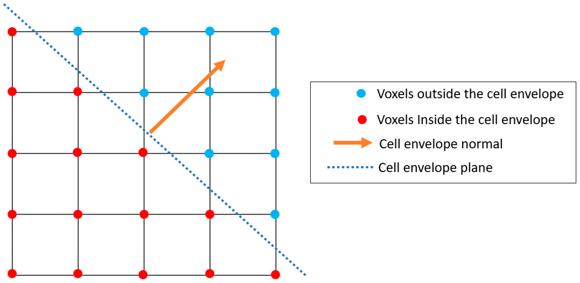
2.1. Representative Volume Element

The representative volume element (RVE) of a lattice is its fundamental unit cell, mathematically depicted by a cell envelope and the lattice configuration, as shown in Figure 3. This figure illustrates the hexagonal lattice topology, with various configurations of cell envelopes, encompassing both orthogonal and non-orthogonal bases. Figure 3b illustrates a discretized two-dimensional hexagonal geometry including a non-orthogonal cell boundary. This figure illustrates three individual kinds of voxels. The green voxels denote the voids within the representative volume element’s cell envelope, with a non-zero volume and void material properties. The green voxels are included solely for the total volume calculation but excluded from the identification of periodic node pairs and the computation of the stiffness matrix. The red voxels denote the discretized geometry, characterized by both non-zero material properties and non-zero volume. The blue voxels are allocated zero volume and zero material properties as they are outside the RVE’s cell envelope. The cell envelope is characterized as a surface with a normal oriented outward from the cell envelope, as seen in Figure 4. According to the specification of the cell envelope’s plane, all voxel elements located outside the cell envelope (on the same side as the normal vector) are eliminated throughout the analysis.

The elastic material characteristic for each voxel is characterized by the two Lame parameters, $\lambda$ and $\mu$, defined as follows:

$$\begin{array}{c}\lambda ={\displaystyle \frac{vE}{\left(1+v\right)\left(1-2v\right)}}\\ \mu ={\displaystyle \frac{E}{2(1+v)}}\end{array}$$

(1)

where $E$ denotes the Young’s modulus of the material and $\nu$ represents the Poisson’s ratio, respectively. The voxel element is defined as an iso-parametric brick element, with orthogonal edges of lengths $l_x$, $l_y$ and $l_z$ aligned to the specified global coordinate system. The individual voxels with non-zero volume within the cell envelope are assigned isotropic material properties, and the stiffness material matrix of the element (${\mathit{C}}^{\left(e\right)}$) is defined as:

$${\mathit{C}}^{\left(e\right)}={\lambda }^{\left(e\right)}·\left[\begin{array}{cccccc}1& 1& 1& 0& 0& 0\\ 1& 1& 1& 0& 0& 0\\ 1& 1& 1& 0& 0& 0\\ 0& 0& 0& 0& 0& 0\\ 0& 0& 0& 0& 0& 0\\ 0& 0& 0& 0& 0& 0\end{array}\right]+{\mu }^{\left(e\right)}·\left[\begin{array}{cccccc}2& 0& 0& 0& 0& 0\\ 0& 2& 0& 0& 0& 0\\ 0& 0& 2& 0& 0& 0\\ 0& 0& 0& 1& 0& 0\\ 0& 0& 0& 0& 1& 0\\ 0& 0& 0& 0& 0& 1\end{array}\right]$$

(2)

where ${\lambda }^{\left(e\right)}$ and ${\mu }^{\left(e\right)}$ are the two lame parameters, and the superscript $\left(e\right)$ denotes that it is defined for individual element.

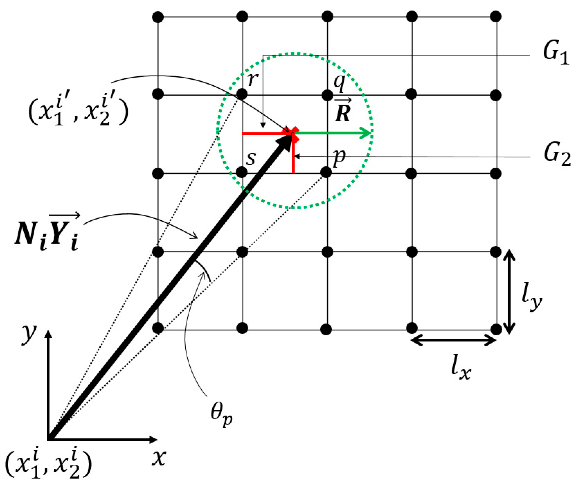
2.2. Discretization and Approximation of the Periodic Boundary Condition

The procedure for establishing the translational periodicity of node pairs involves translating a node’s coordinates using the periodic basis vector and thereafter identifying the nearest node within a specified search radius.

A physical quantity of a periodic structure can be expressed as:

$$\mathcal{F}\left(\mathit{x}+\mathit{N}\mathit{Y}\right)=\mathcal{F}\left(\mathit{x}\right)$$

(3)

where $\mathit{N}=\lceil {\mathrm{n}}_1,{\mathrm{n}}_2,{\mathrm{n}}_3\rfloor$ is a $3\times 3$ diagonal matrix which consists of arbitrary integer values, $\mathit{x}={\left[x_1,x_2,x_3\right]}^T$ is the position vector of a point where the physical quantity $\mathcal{F}$ is evaluated and $\mathit{Y}={\left[Y_1, Y_2, Y_3\right]}^T$ is a vector that denotes the period of the structure, where this value could be a scalar, a vector or a tensor function of $\mathit{x}$ [28].

Using the previous equation, the stress tensor (${\sigma }_{ij}$) of a periodic structure can then be defined as:

$$\begin{array}{l}{\mathit{\sigma }}_{\mathit{i}\mathit{j}}={\mathit{C}}_{\mathit{i}\mathit{j}\mathit{k}\mathit{l}}\left(\mathit{x}\right){\mathit{\epsilon }}_{\mathit{k}\mathit{l}}={\mathit{C}}_{\mathit{i}\mathit{j}\mathit{k}\mathit{l}}(\mathit{x}+\mathit{N}\mathit{Y}){\mathit{\epsilon }}_{\mathit{k}\mathit{l}}\\ i,j,k,l,p,q\in \{1,2,3\}\end{array}$$

(4)

where ${\mathit{C}}_{\mathit{i}\mathit{j}\mathit{k}\mathit{l}}$ is the stiffness tensor and ${\mathit{\epsilon }}_{\mathit{k}\mathit{l}}$ is the strain tensor. By definition of $\mathit{x},\mathit{N}$ and $\mathit{Y}$, the stiffness tensor ${\mathit{C}}_{\mathit{i}\mathit{j}\mathit{k}\mathit{l}}$ can be expanded as

$$\begin{array}{l}{\mathit{C}}_{\mathit{i}\mathit{j}\mathit{k}\mathit{l}}\left({\mathrm{x}}_1+{\mathrm{n}}_1{\mathrm{Y}}_1,{\mathrm{x}}_2+{\mathrm{n}}_2{\mathrm{Y}}_2,{\mathrm{x}}_3+{\mathrm{n}}_3{\mathrm{Y}}_3\right)={\mathit{C}}_{\mathit{i}\mathit{j}\mathit{k}\mathit{l}}\left({\mathrm{x}}_1,{\mathrm{x}}_2,{\mathrm{x}}_3\right)\\ i,j,k,l \in \{1,2,3\}\end{array}$$

(5)

The voxel element’s nodes are discretized with the nodal coordinates ($x_1^i, x_2^i, x_3^i$) of the $i$^th node is defined as:

$$\begin{array}{l}\left(\begin{array}{c}{x}_1^i\\ x_2^i\\ x_3^i\end{array}\right)=\left(\begin{array}{c}{A}_1{l}_x+O_x\\ A_2{l}_y+O_y\\ A_3{l}_z+O_z\end{array}\right), \mathrm{w}\mathrm{h}\mathrm{e}\mathrm{r}\mathrm{e} \begin{array}{c}{A}_1=\left\{0,1, 2, \dots , x_{divs}\right\}\\ A_2=\left\{0, 1, 2, \dots , y_{divs}\right\}\\ A_3=\left\{0, 1, 2, \dots , z_{divs}\right\}\end{array},\\ i=\{1, 2, \dots , \left(x_{divs}+1\right)\times \left(y_{divs}+1\right)\times \left(z_{divs}+1\right)\}\end{array}$$

(6)

where $A_1,A_2,$ and $A_3$ are integers, and {$O_x, O_y, O_z$} denotes the origin; the $i$ superscript corresponds to the node numbers. $l_x$, $l_y$, and $l_z$ represents the lengths of the voxel along the global cartesian x, y, and z axes, respectively; the $x_{divs}$, $y_{divs}$ and $z_{divs}$ are then integers indicating the number of voxel discretization along the global cartesian x, y, and z axes, respectively. Generally, $l_x$, $l_y$, and $l_z$ are uniform across for all the voxels and can be computed as:

$$\left(\begin{array}{c}{l}_x\\ l_y\\ l_z\end{array}\right)=\left(\begin{array}{c}{\displaystyle \frac{\max \left({\mathrm{x}}_1^i\right)-\mathrm{m}\mathrm{i}\mathrm{n}\left({\mathrm{x}}_1^i\right)}{x_{divs}}}\\ {\displaystyle \frac{\max \left({\mathrm{x}}_2^i\right)-\mathrm{m}\mathrm{i}\mathrm{n}\left({\mathrm{x}}_2^i\right)}{y_{divs}}}\\ {\displaystyle \frac{\max \left({\mathrm{x}}_3^i\right)-\mathrm{m}\mathrm{i}\mathrm{n}\left({\mathrm{x}}_3^i\right)}{z_{divs}}}\end{array}\right) \mathrm{a}\mathrm{n}\mathrm{d} \left(\begin{array}{c}{O}_x\\ O_y\\ O_z\end{array}\right)=\left(\begin{array}{c}\mathrm{m}\mathrm{i}\mathrm{n}\left({\mathrm{x}}_1^i\right)\\ \mathrm{m}\mathrm{i}\mathrm{n}\left({\mathrm{x}}_2^i\right)\\ \mathrm{m}\mathrm{i}\mathrm{n}\left({\mathrm{x}}_3^i\right)\end{array}\right).$$

(7)

The periodicity vector $\mathit{Y}$ can be discretized on a cartesian grid as:

$$\mathit{Y}=\left(\begin{array}{c}{\mathrm{Y}}_1\\ {\mathrm{Y}}_2\\ {\mathrm{Y}}_3\end{array}\right)=\left(\begin{array}{c}{B}_1{l}_x\\ B_2{l}_y\\ B_3{l}_z\end{array}\right)+\left(\begin{array}{c}{G}_1\\ G_2\\ G_3\end{array}\right): \begin{array}{c}{B}_1, B_2, B_3\in \mathbb{Z}\\ \begin{array}{c}{G}_1, G_2, G_3\in \mathbb{R}\\ G_1<l_x, G_2<l_y, G_3<l_z,\end{array}\end{array}$$

(8)

where $G_1,G_2,$ and $G_3$ are the remainder or the residual which are smaller than the lengths of a voxel along $l_x,l_y,$ or $l_z$ respectively; and $B_1,B_2,$ and $B_3$ are integers.

For every voxel node, as created using Equation $\left(6\right)$, that makes up the RVE’s cell envelope, there exists a corresponding periodic node pair that is likewise included in the discretized RVE’s cell envelope.

If any of the residuals $G_i$ in Equation $\left(8\right)$ are non-zero, it is impossible to identify the precise node within the voxels, as illustrated in Figure 5, resulting in the approximation of periodic node pairings and subsequent numerical inaccuracies. Estimating the position of the periodic node pair entails disregarding the residuals ($G_i$). A perfect voxel mesh can be achieved by reducing the residual term. In an orthogonal periodic basis aligned with the global coordinate system, the residuals are inherently zero. However, for an RVE with a non-orthogonal periodic basis or a rotated orthogonal periodic basis (or periodic bases that are not collinear with the global discretization axis), the $x_{divs}$, $y_{divs}$ and $z_{divs}$ must be tuned in order to minimize the residuals as necessary.

To identify the periodic node pair for an RVE with a non-orthogonal periodic basis, a localized search must be performed within a radius of $R$, ensuring that at least one point is encompassed within the specified search radius, as illustrated in Figure 5. Failure to locate the periodic node for the boundary node, or misidentification of the node pair, may result in minor numerical inaccuracies. A recommended search radius is proposed as:

$$R=\mathrm{m}\mathrm{a}\mathrm{x}\left(\begin{array}{c}0.51\left({\displaystyle \frac{l_x+l_y+l_z}{3}}\right)\\ 0.51 max\left(l_x,l_y,l_z\right)\\ 0.51\left(\sqrt{l_x^2+l_y^2+l_z^2}\right)\end{array}\right),$$

(9)

The proposed search radius is based on factors such as using a little more than the half of the average lengths, half of the maximum lengths, or half of the largest diagonal lengths. These were chosen to provide an adequate node pair matching based on any arbitrary voxel aspect ratios.

For a coarse mesh, instead of utilizing the proposed radius constraint in Equation $\left(9\right)$, it is recommended to utilize angular constraints, when the angle ${\theta }_p$ depicted in Figure 5 exceeds 5°. The angle ${\theta }_p$, depicted in Figure 5, can be determined by executing the dot product operation between the two normalized vectors $\overrightarrow{\mathit{Y}}$ and $\overrightarrow{x^{i}p}$. The misalignment between the periodic basis and the voxel’s natural element coordinate system results in minor numerical inaccuracies, as elaborated in Section 3.2 and Section 3.3.

In order to evaluate the periodicity of the lattice, the untranslated original nodal coordinates of all voxels are used to construct a k-d tree, facilitating the implementation of a fast-nearest neighbor algorithm [64]. Then, an offset is applied to all voxel coordinates. The offset is calculated based on integer linear combinations (−1, 0, and +1) of the basis vectors. This linear combination process is used to evaluate all the periodicity vectors. This lets us determine all periodic node pairs for a given node.

Then, the offset nodes are matched to the original nodes based on the nearest point within a specified minimum distance $R$ and a minimum angle ${\theta }_p$. Unit cells featuring an orthogonal periodic basis that corresponds with the voxel’s natural coordinate system are exempt from minimum distance and angular constraints. In a lattice geometry with a periodic basis that does not align as an integer multiple of the voxel’s native coordinate system, identifying the periodic nodal pair necessitates an extra step, as the offset coordinate does not overlap with the second nodal pair. Consequently, a local search must be performed to identify the nearest point adhering to the minimal distance and angle constraints described in Equation $\left(9\right)$. As a rule of thumb, there must be a minimum of 5 voxels discretization per truss radius or thickness (shellular or plate) to properly evaluate the periodic boundary condition. If the number of discretization are smaller, the voxel centers may not be detected to be within the desired distance, and may cause geometrical discontinuity within the RVE during the discretization process.

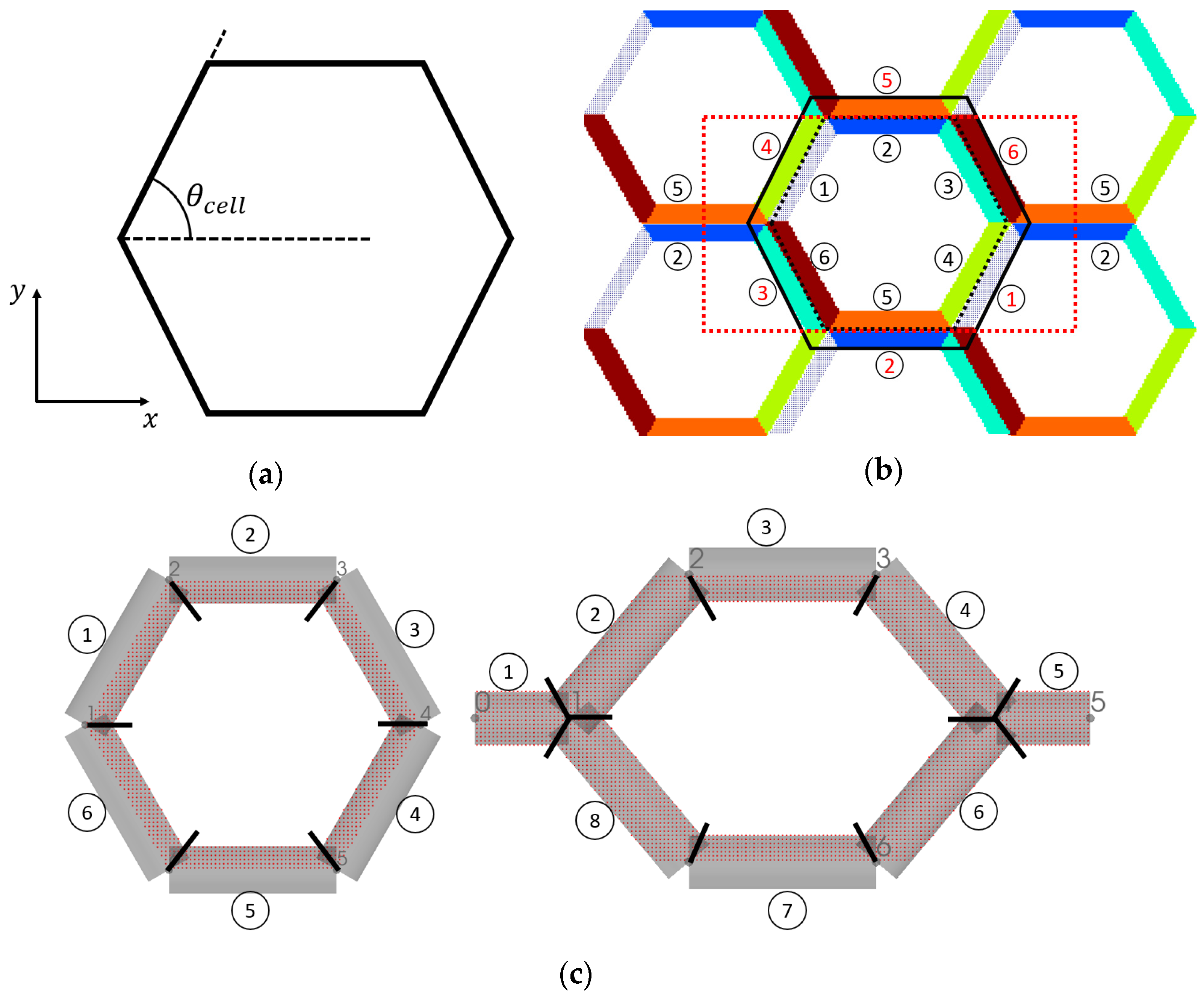
2.3. Multi-Material Assignment to a Discretized Lattice Structure

For a lattice material made from a single isotropic material, its homogenized TEC will be constant, and does not change with the relative density of the lattice. To create a lattice with variable thermal expansion coefficient, two or more materials with varying thermal expansion coefficients must exist within a lattice structure. Thus, for a discretized lattice, the distribution of the material for the discretized element has a large impact on the calculated results. In this paper, the material distribution for a truss lattice near a joint is based on its orientation, where the truss is truncated based on the bisector plane formed with the most adjacent truss, which is shown in Figure 6c. The tessellated closed hexagon lattice is shown in Figure 6b, where the splitting of the truss based on the bisector plane is shown to produce sharp corners, which is not a realistic representation for manufacturing purposes. When considering the periodicity, the trusses with ID of the closed hexagon lattices forms the following groups: [1, 4], [2, 5] and [3, 6]. These correspond to the orthogonal hexagon’s groups of [2, 6], [1, 3, 5, 7], and [4, 8], respectively. Thus, for a bi-material hexagon lattice, there are eight ($2^3$) possible configurations available.

2.4. Asymptotic Homogenization

The AH process is based on the double scale expansion theory [28,29,30,31,60,61]. The parent material property for the individual voxel is defined using the two Lame’s parameters, shown in Equation (1).

As explained above, the voxel element is formulated as an iso-parametric brick element. The individual voxels with non-zero volume that are inside the cell envelope are treated to have an isotropic material property, and the element’s stiffness material matrix (${\mathit{C}}^{\left(e\right)}$) is formulated as shown in Equation (2).

The strain–displacement matrix (${\mathbf{B}}_e$) and the material matrix (${\mathit{C}}^{\left(e\right)}$) of the iso-parametric voxel element are utilized to ascertain the local element stiffness matrix (${\mathbf{k}}_e$). The element stiffness matrix was divided into two components (${\mathbf{k}}_{\lambda }$ and ${\mathbf{k}}_{\mu }$, corresponding to Lame’s parameters in ${\mathit{C}}^{\left(e\right)}$). This was executed for computational convenience, facilitating the support of various materials by altering ${\lambda }^{\left(e\right)}$ and ${\mu }^{\left(e\right)}$. Upon implementing the periodic boundary condition through the coupling of degrees of freedom for the periodic node pairs, the global stiffness matrix ($\mathbf{K}$) is formulated as follows:

$$\mathbf{K}=\sum _{e=1}^N{\mathbf{k}}_{\mathbf{e}}=\sum _{e=1}^N{\int }_{V_e}{\mathbf{B}}_e^T{\mathbf{C}}^{\left(e\right)}{\mathbf{B}}_e\mathrm{d}{V}_e=\sum _{e=1}^N\left({\lambda }^{\left(e\right)}{\mathbf{k}}_{\lambda }+{\mu }^{\left(e\right)}{\mathbf{k}}_{\mu }\right)$$

(10)

The integration above is carried out using three-point Gaussian quadrature [65]. Implementing periodic boundary conditions will couple the degrees of freedoms (DOFs) for the nodes within the cell envelope, hence reducing the overall number DOFs. The global stiffness matrix for this system, incorporating periodic boundary conditions, will be designated as the reduced global stiffness matrix.

2.4.1. Thermal Expansion Homogenization

The homogenized thermal stress vector can be determined as [31,58],

$$\begin{array}{c}{\beta }_{ij}^H={\displaystyle \frac{1}{\left|V_{RVE}\right|}}{\displaystyle \sum _{e=1}^N}{\int }_{V_e}{\left({\mathsf{\Gamma }}_e^0-{\mathsf{\Gamma }}_{\mathrm{e}}\right)}^T{\mathbf{k}}_e\left({\mathit{\chi }}_e^{0\left(ij\right)}-{\mathit{\chi }}_e^{\left(ij\right)}\right)\mathrm{d}{V}_e\\ i,j \in \{1,2,3,\}\end{array}$$

(11)

where $\beta$ represents the thermal stress vector; $V_{RVE}$ denotes the volume of the representative volume element; $V_e$ signifies the volume of the voxel element; ${\mathit{\chi }}_e^0$ and ${\mathit{\chi }}_{\mathit{e}}$ represent the macro and micro displacements resulting from imposed unit stresses, and ${\mathsf{\Gamma }}_{\mathbf{e}}$ is the scalar temperature field. The macro and micro temperatures are calculated by solving the subsequent equations:

$${\mathbf{k}}_{\mathbf{e}}{\mathsf{\Gamma }}_e^0={\mathbf{f}}_{\alpha }$$

(12)

$$\mathbf{K}{\mathsf{\Gamma }}_e^i={\mathbf{f}}_{\mathit{\alpha }}^i$$

(13)

where ${\mathbf{f}}_{\alpha }$ is the unit thermal load corresponding to six unit-thermal strain, which can be calculated as:

$$\begin{array}{c}{\mathbf{f}}_{\alpha }={\displaystyle \sum _e}{\int }_{{\mathrm{V}}_{\mathrm{e}}}{\mathbf{B}}_{\mathrm{e}}^{\mathrm{T}}{\mathbf{C}}^{\left(\mathrm{e}\right)}{\mathsf{\alpha }}_{\mathrm{e}}^{\mathrm{i}}\mathrm{d}{\mathrm{V}}_{\mathrm{e}}, i=1,\dots ,6\\ {\alpha }^1={\left(1,0,0,0,0,0\right)}^T, {\alpha }^2={\left(0,1,0,0,0,0\right)}^T,\dots , {\alpha }^6={\left(0,0,0,0,0,1\right)}^T\end{array}$$

(14)

The homogenized thermal expansion (${\mathit{\alpha }}^H$) can be calculated by solving the following equation [31,58]:

$${\mathit{C}}_{\mathit{i}\mathit{j}}^H{\mathit{\alpha }}_i^H={\mathit{\beta }}_{\mathit{j}}^H, i,j\in \{1,2,3\}$$

(15)

where the superscript $H$ denotes the homogenized quantity; the homogenized macroscopic elasticity tensor (${\mathit{C}}_{\mathit{i}\mathit{j}}^H$) can then be written as [31,32]:

$$\begin{array}{c}{\mathit{C}}_{\mathit{i}\mathit{j}}^H={\mathit{E}}_{\mathit{i}\mathit{j}\mathit{k}\mathit{l}}^{\mathit{H}}={\displaystyle \frac{1}{\left|V\right|}}{\int }_V{\mathit{E}}_{\mathit{p}\mathit{q}\mathit{r}\mathit{s}}\left({\mathit{\epsilon }}_{\mathit{p}\mathit{q}}^{\mathbf{0}\left(\mathit{i}\mathit{j}\right)}-{\mathit{\epsilon }}_{\mathit{p}\mathit{q}}^{\left(\mathit{i}\mathit{j}\right)}\right)\left({\mathit{\epsilon }}_{\mathit{r}\mathit{s}}^{\mathbf{0}\left(\mathit{k}\mathit{l}\right)}-{\mathit{\epsilon }}_{\mathit{r}\mathit{s}}^{\left(\mathit{k}\mathit{l}\right)}\right)\mathrm{d}V\\ i,j,k,l,p,q,r,s \in \{1,2,3\}\end{array}$$

(16)

where $V$ denotes the volume of the base RVE, ${\mathit{E}}_{\mathit{p}\mathit{q}\mathit{r}\mathit{s}}$ signify the locally variable stiffness tensor, ${\epsilon }_{pq}^{0\left(ij\right)}$ indicates the macroscopic strain, and ${\mathit{\epsilon }}_{\mathit{p}\mathit{q}}^{\left(\mathit{i}\mathit{j}\right)}$ represents the microscopic strain (locally periodic). Additional information regarding 3D and 2D voxels is available in references [31,32].

${\mathit{\epsilon }}_{\mathit{p}\mathit{q}}^{\left(\mathit{i}\mathit{j}\right)}$ is defined as:

$${\mathit{\epsilon }}_{\mathit{p}\mathit{q}}^{\left(\mathit{i}\mathit{j}\right)}={\mathit{\epsilon }}_{\mathit{p}}\left({\mathit{\chi }}^{\mathit{i}\mathit{j}}\right)={\displaystyle \frac{1}{2}}\left({\mathit{\chi }}_{\mathit{p},\mathit{q}}^{\mathit{i}\mathit{j}}+{\mathit{\chi }}_{\mathit{q},\mathit{p}}^{\mathit{i}\mathit{j}}\right), p,q \in \{1,2,3\}$$

(17)

By resolving the elasticity equations with specified macroscopic strains below, this yields displacement fields ${\mathit{\chi }}^{\mathit{k}\mathit{l}}$:

$$\begin{array}{c}{\int }_{\mathit{V}}{\mathit{E}}_{\mathit{i}\mathit{j}\mathit{p}\mathit{q}}{\mathit{\epsilon }}_{\mathit{i}\mathit{j}}\left(\mathit{v} \right){\mathit{\epsilon }}_{\mathit{p}\mathit{q}}\left({\mathit{x}}^{\mathit{k}\mathit{l}}\right)dV={\int }_{\mathit{V}}{\mathit{E}}_{\mathit{i}\mathit{j}\mathit{p}\mathit{q}}{\mathit{\epsilon }}_{\mathit{i}\mathit{j}}\left(\mathit{v} \right){\mathit{\epsilon }}_{\mathit{p}\mathit{q}}^{\mathbf{0}\left(\mathit{k}\mathit{l}\right)}dV\\ i,j,k,l,p,q\in \{1,2,3\}\end{array}$$

(18)

where $\mathit{v}$ is the virtual displacement field.

2.4.2. Thermal Conduction Homogenization

The thermal conductivity homogenization is very similar to the thermal expansion homogenization. The homogenized thermal conductivity (${\mu }_{ij}^H$) can be found as [31,32],

$$\begin{array}{c}{\mu }_{ij}^H={\displaystyle \frac{1}{\left|V_{RVE}\right|}}{\displaystyle \sum _{e=1}^N}{\int }_{V_e}{\left({\mathit{T}}_e^{0\left(i\right)}-{\mathit{T}}_e^{\left(i\right)}\right)}^T{\mu }_{lm}\left({\mathit{T}}_e^{0\left(j\right)}-{\mathit{T}}_e^{\left(j\right)}\right)\mathrm{d}{V}_e\\ i,j\in \{1,2,3\}\end{array}$$

(19)

where ${\mathsf{\mu }}_{lm}$ is the thermal conductivity stiffness matrix found using Equation $\left(20\right)$, and ${\mathbf{T}}_{\mathbf{e}}$ is the temperature field. For thermal conductivity, the element thermal conductivity matrix (${\mathit{\mu }}_{cond}^{\left(e\right)}$) is formulated as [31,32,42]

$${\mathit{\mu }}_{cond}^{\left(e\right)}={\lambda }_{cond}^{\left(e\right)}\left[\begin{array}{cccccc}1& 1& 0& 0& 0& 0\\ 0& 1& 0& 0& 0& 0\\ 0& 0& 1& 0& 0& 0\\ 0& 0& 0& 0& 0& 0\\ 0& 0& 0& 0& 0& 0\\ 0& 0& 0& 0& 0& 0\end{array}\right]$$

(20)

where ${\lambda }_{cond}^{\left(e\right)}$ is the thermal conductivity for an isotropic material. This is used to calculate the global thermal conductivity matrix using Equation $\left(10\right)$, replacing ${\mathbf{k}}_{\mathbf{e}}$ with ${\mathit{\mu }}_{cond}^{\left(e\right)}$, but limited to three DOF instead of six per node.

3. Verification and Validation

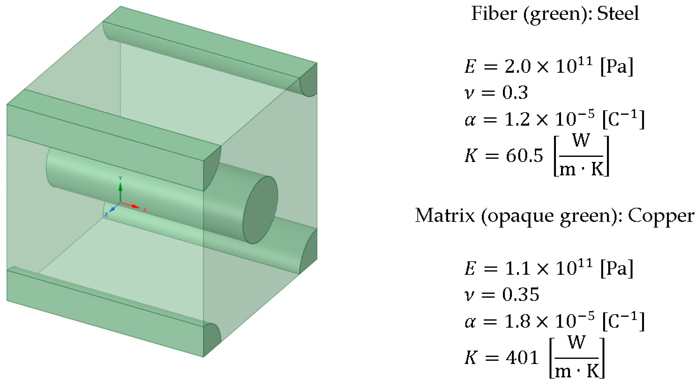
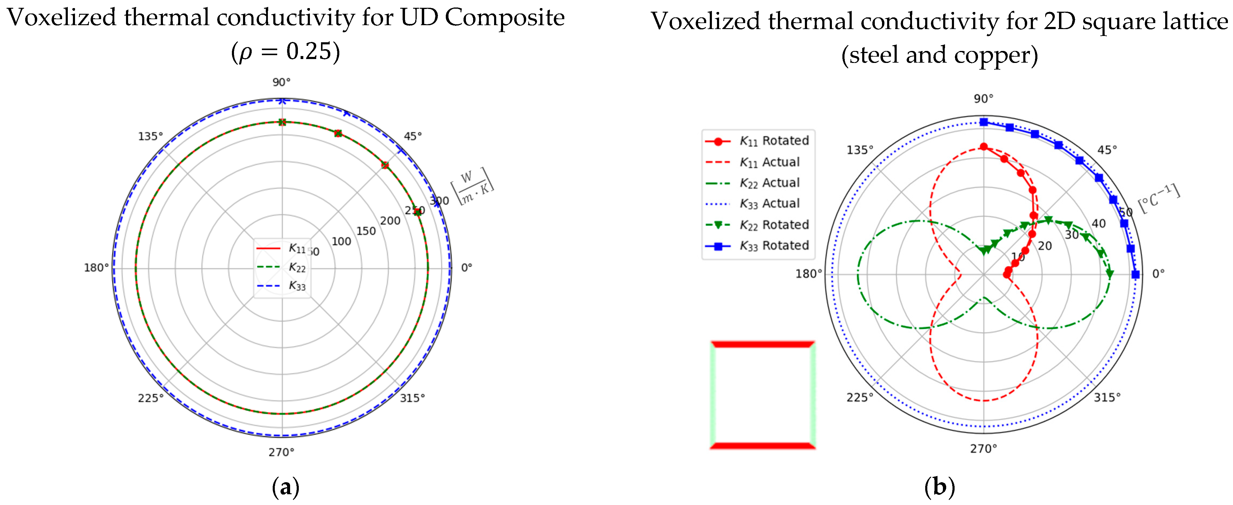
3.1. Uni-Directional Composite

To achieve varied thermal expansion in a periodic medium, it is necessary to utilize two or more materials with distinct thermal expansion coefficients. The thermal expansion of an unconstrained lattice composed of a single material remains invariant with respect to relative density. Thermal expansion and thermal conductivity homogenization were conducted for a Uni-Directional (UD) composite material, as illustrated in Figure 7. To validate the homogenization of thermal expansion and thermal conductivity, ANSYS 2021 R2 is utilized which supports multi material weaved composites such as fiber in matrix/epoxy. Therefore, unidirectional composite material, with fibers oriented in the x-direction, was employed. Copper and steel were selected arbitrarily for the matrix and fiber, respectively. Steel was chosen because it is a common material, and copper was chosen for its high thermal conductivity.

Figure 8 presents the results obtained from the homogenization of the thermal properties. The results obtained from the homogenization framework demonstrate a high degree of comparability with ANSYS, effectively calculating both the thermal expansion and thermal conductivity of the bi-material. The maximum errors based on the plots in Figure 8 were below 6% for thermal conductivity and below 1% for thermal expansion. The orthogonality of the periodicity vectors results in the primary error contribution arising from the discretization of geometry into voxels, leading to deviations in the relative density of the fiber.

Figure 9 displays an anisotropic representation of the thermal conductivity matrix. The scattered points denote the specific conductivity values for a geometry that has undergone rotation and discretization.

$$\begin{array}{c}{{\kappa }_{ij}^H}^{\prime }={\displaystyle \frac{\mathbf{J}{\kappa }_{ij}^H{\mathbf{J}}^T}{\det \left(\mathbf{J}\right)}}\\ \mathbf{J}=\left[\begin{array}{ccc}\cos \left(\theta \right)& \sin \left(\theta \right)& 0\\ -\sin \left(\theta \right)& \cos \left(\theta \right)& 0\\ 0& 0& 1\end{array}\right], 0\le \theta \le 2\pi \end{array}$$

(21)

The anisotropy plot is derived by extracting the principal diagonal of ${{\kappa }_{ij}^H}^{\prime }$ from Equation $\left(21\right)$. The initial conductivity matrix is rotated about the z-axis (the out-of-plane axis for the two-dimensional square lattice). The rotated values correspond closely with the original anisotropy figure, and the minor discrepancies are from variations in relative density throughout the voxel discretization process. When the rotation is applied to the conductivity matrix, it is equivalent to rotating the physical material. For an anisotropic material, heat does not flow equally in all directions; thus, rotating the tensor shows how preferred heat flow directions change with orientation, which can be used to produce the anisotropy plots as shown in Figure 9.

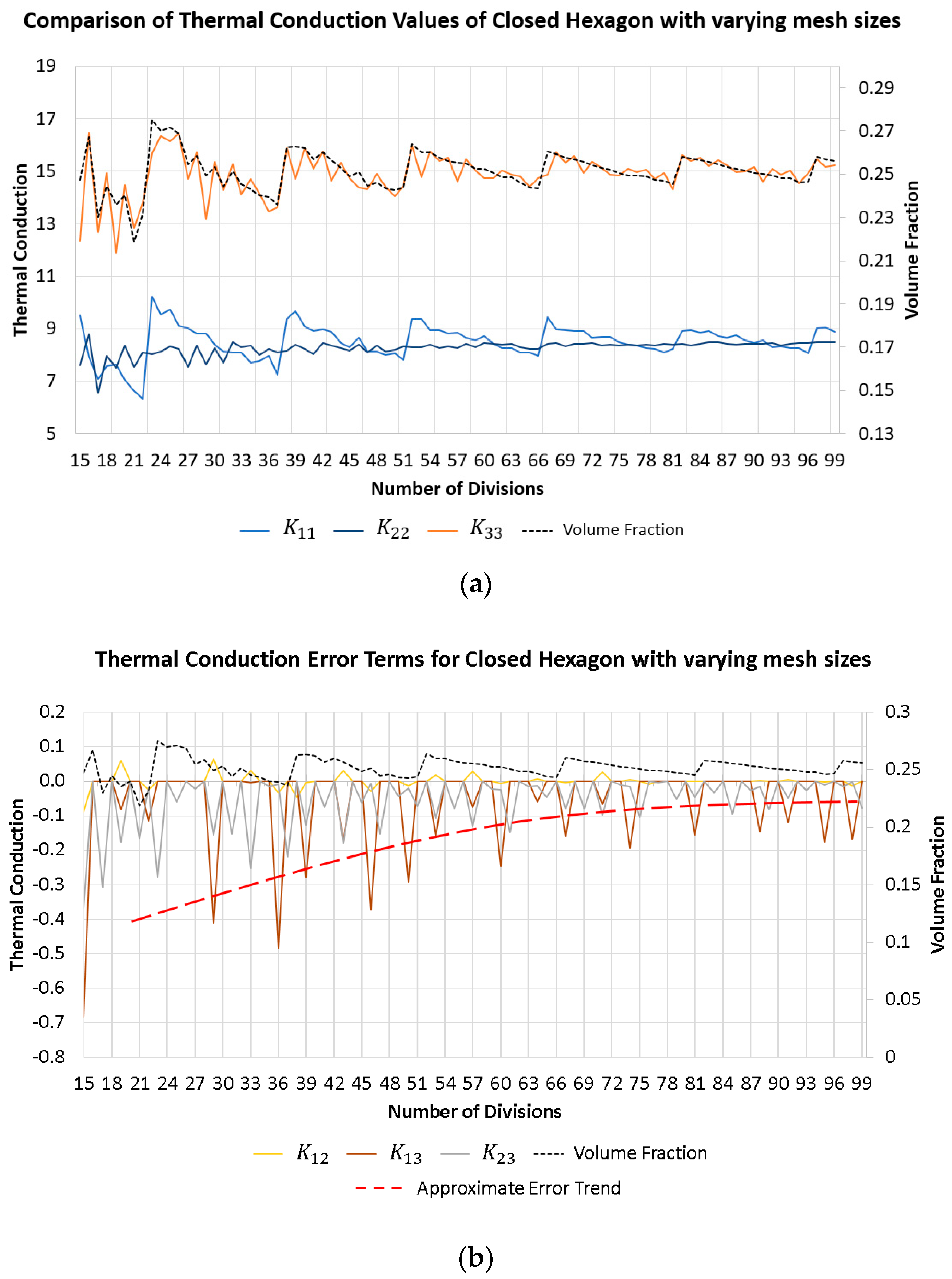
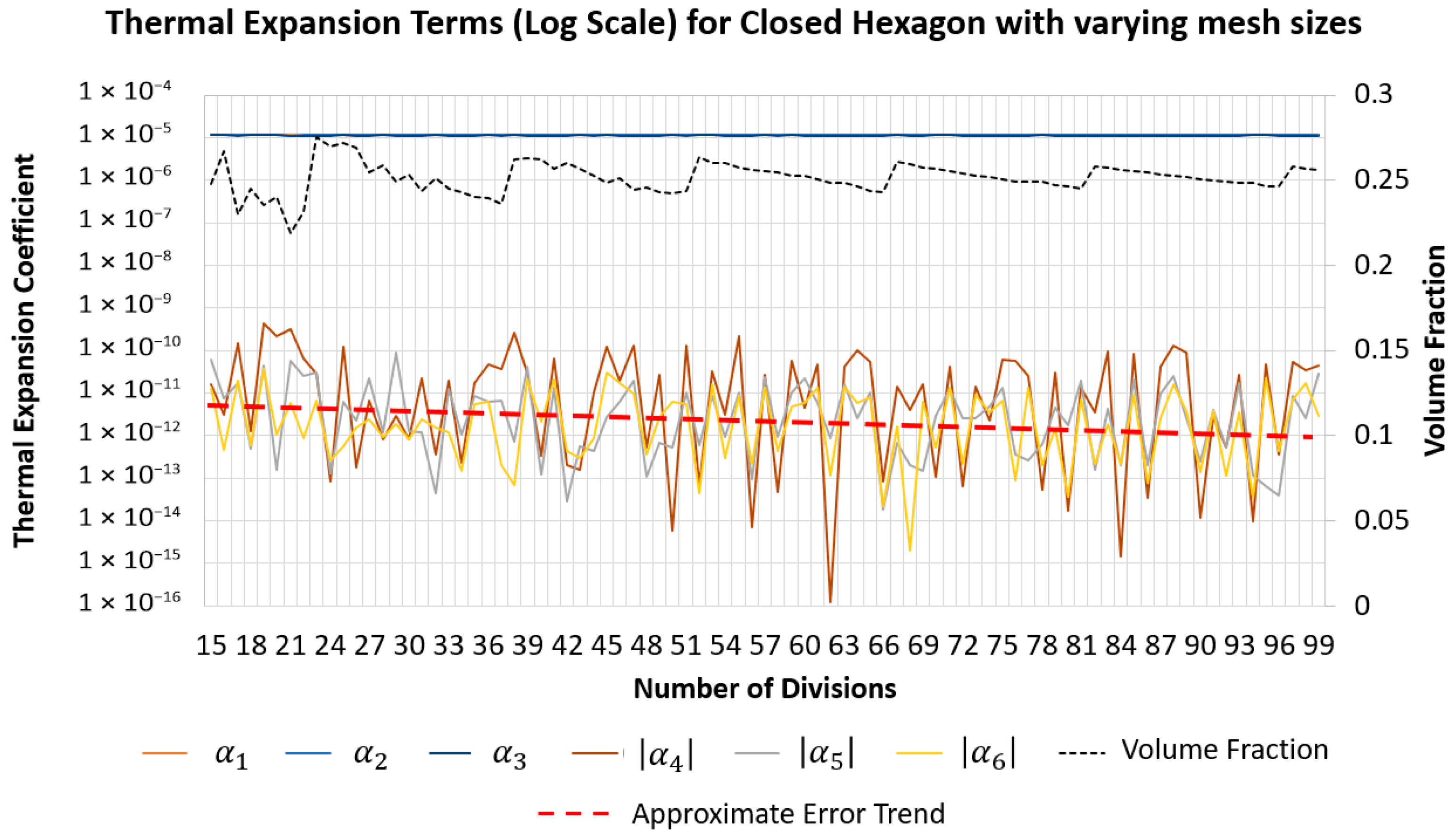
3.2. Grid Convergence

For a bi-material hexagon lattice, the homogenized thermal conduction matrix ${\kappa }_{ij}^H$ and the thermal expansion coefficients ${\alpha }_i^H$ must have the following zero and non-zero terms:

$$\begin{array}{c}{\kappa }_{ij}^H=\left[\begin{array}{ccc}{\kappa }_{11}& 0.& 0.\\ 0.& {\kappa }_{22}& 0.\\ 0.& 0.& {\kappa }_{33}\end{array}\right]\\ {\alpha }_i^H=\left[\begin{array}{ccc}\begin{array}{cc}{\alpha }_1& {\alpha }_2\end{array}& \begin{array}{cc}{\alpha }_3& 0.\end{array}& \begin{array}{cc}0.& 0.\end{array}\end{array}\right]\end{array}$$

(22)

But due to the approximation of the periodic boundary condition, the zero terms will be replaced with small non-zero numbers. The small non-zero terms for the thermal conduction and thermal expansion are plotted in Figure 10 and Figure 11, respectively. In this simulation, the radius of the hexagon lattice’s truss is fixed, and the hexagon was discretized to have a voxel aspect ratio of unity.

The main diagonal terms of the thermal conduction matrix, plotted in Figure 10a, closely follow the general trend of the volume fraction, but the ‘high frequency’ jitter in the plots is mainly caused by the approximation of the periodic boundary condition. The variation in the volume fraction is due to the discretization process, where the volume fraction jumps safter increasing the number of discretization by one because the center of the voxels suddenly crossed the bounds of the cell envelope plane definition, as shown in Figure 3b and Figure 4.

3.3. Numerical Errors Due to Approximating Periodicity

This section describes a 2D hexagonal unit cell that is meshed with an equal number of divisions along the global cartesian x and y axes, and a single element along the z axis. The subsequent term (${\tau }_e$), visualized in Figure 12, is defined as:

$$\begin{array}{c}{\mathit{\tau }}_{\mathit{e}}^{\left(\mathit{i}\right)\left(\mathit{j}\right)}={\displaystyle \frac{1}{{\mathit{\mu }}_{\mathit{i}\mathit{j}}^{\mathit{H}}}}{\int }_{V_e}{\left({\mathit{T}}_e^{0\left(i\right)}-{\mathit{T}}_e^{\left(i\right)}\right)}^T{\mathit{\mu }}_{\mathit{l}\mathit{m}}\left({\mathit{T}}_e^{0\left(j\right)}-{\mathit{T}}_e^{\left(j\right)}\right)\mathrm{d}{V}_e\\ i,j\in \{1,2,3\}\end{array}$$

(23)

where ${\tau }_e$ denotes the contribution of element $e$ to the homogenized conduction matrix ${\mu }_{ij}^H$, normalized by the total ${\mu }_{ij}^H$. Visualizing ${\tau }_e$ for each element allows for the identification of elements that may contribute to the numerical errors illustrated in Figure 12. The color scheme implemented in Figure 12 is designed so that the maximum absolute value determines the boundaries for both the positive (red) and negative (blue) regions of the plot. Values that are near zero are represented in white.

Additionally, Figure 10 illustrates that an increase in voxel discretization leads to a reduction in the small non-zero components of the $\left[{\kappa }_{ij}^H\right]$ tensor, as each voxel contributes a diminished value resulting from the smaller voxel volume. Figure 13 illustrates that, for the hexagon with a larger voxel size, the residual terms arise from the voxels along the edges, which are influenced by imperfect periodic boundary conditions. The refined hexagon lattice depicted in Figure 13b exhibits a smaller ratio of edge voxels compared to the hexagon with a larger voxel size, resulting in a reduced contribution of the residual error.

4. Results and Discussion

In this section, the conductivity and thermal expansion is presented for the full permutation of bi-material lattice configuration for varying cell angles at a volume fraction of 0.3. The materials considered in this study are steel and invar, with the properties tabulated in

Table 1. Material properties of steel and invar used in the analysis.

Steel [59]	Invar 2036 [66]
$E=200\times {10}^9 \left[\mathrm{P}\mathrm{a}\right]$	$E=140\times {10}^9 \left[\mathrm{P}\mathrm{a}\right]$
$\nu =0.3$	$\nu =0.25$
$\alpha =1.2\times {10}^{-5} \left[{\mathrm{C}}^{-1}\right] \left(\mathrm{f}\mathrm{r}\mathrm{o}\mathrm{m} 20° \mathrm{t}\mathrm{o} 150 °\mathrm{C}\right)$	$\alpha =2.0\times {10}^{-6} \left[{\mathrm{C}}^{-1}\right]\left(\mathrm{f}\mathrm{r}\mathrm{o}\mathrm{m} 20° \mathrm{t}\mathrm{o} 150 °\mathrm{C}\right)$
$K=60.5 \left[{\displaystyle \frac{\mathrm{W}}{\mathrm{m}\mathrm{K}}}\right]$	$K=10.0 \left[{\displaystyle \frac{\mathrm{W}}{\mathrm{m}\mathrm{k}}}\right]$

. Steel was chosen due to it being a common material, and its counterpart Invar was chosen due to its low thermal expansion coefficient, which is typically used in precision optics.

The cell angles explored were in 10° increments, from 30° to 80°, inclusively. A subset of the cell angle configurations are visualized in Figure 14.

The Truss IDs are grouped based on the truss IDs labelled in Figure 6, where groups 1, 2, and 3 corresponds to the trusses with the following IDs: [1, 4], [2, 5] and [3, 6] for closed hexagon; and [2, 6], [1, 3, 5, 7], and [4, 8] for open hexagon, respectively. The configuration number for the material assignment are tabulated in

Table 2. Material assignment.

Configuration Number	Group 1	Group 2	Group 3
0	Steel	Steel	Steel
1	Steel	Steel	Invar
2	Steel	Invar	Steel
3	Steel	Invar	Invar
4	Invar	Steel	Steel
5	Invar	Steel	Invar
6	Invar	Invar	Steel
7	Invar	Invar	Invar

.

4.1. Variation in Thermal Expansion w.r.t Cell Angle for Multiple Material Configuration

The TECs in the x, y, and z-axes are shown in Figure 15. It is shown here that for certain configurations of the bi-material hexagonal lattice, large positive, small negative and zero thermal expansion coefficients can be obtained by changing the internal cell angle. The mechanism behind the zero and negative thermal expansion for the hexagon lattice is very similar to the mechanism in the auxetic lattice, where due to the differences in expansion/contraction of trusses, this leads to auxetic behavior in multi-material lattices.

Furthermore, due to the discretization of the lattice geometry, and considering only a single layer, and assuming a periodicity in the out-of-plane (z) direction, the thermal expansion along the z-direction (${\alpha }_3$) remains constant.

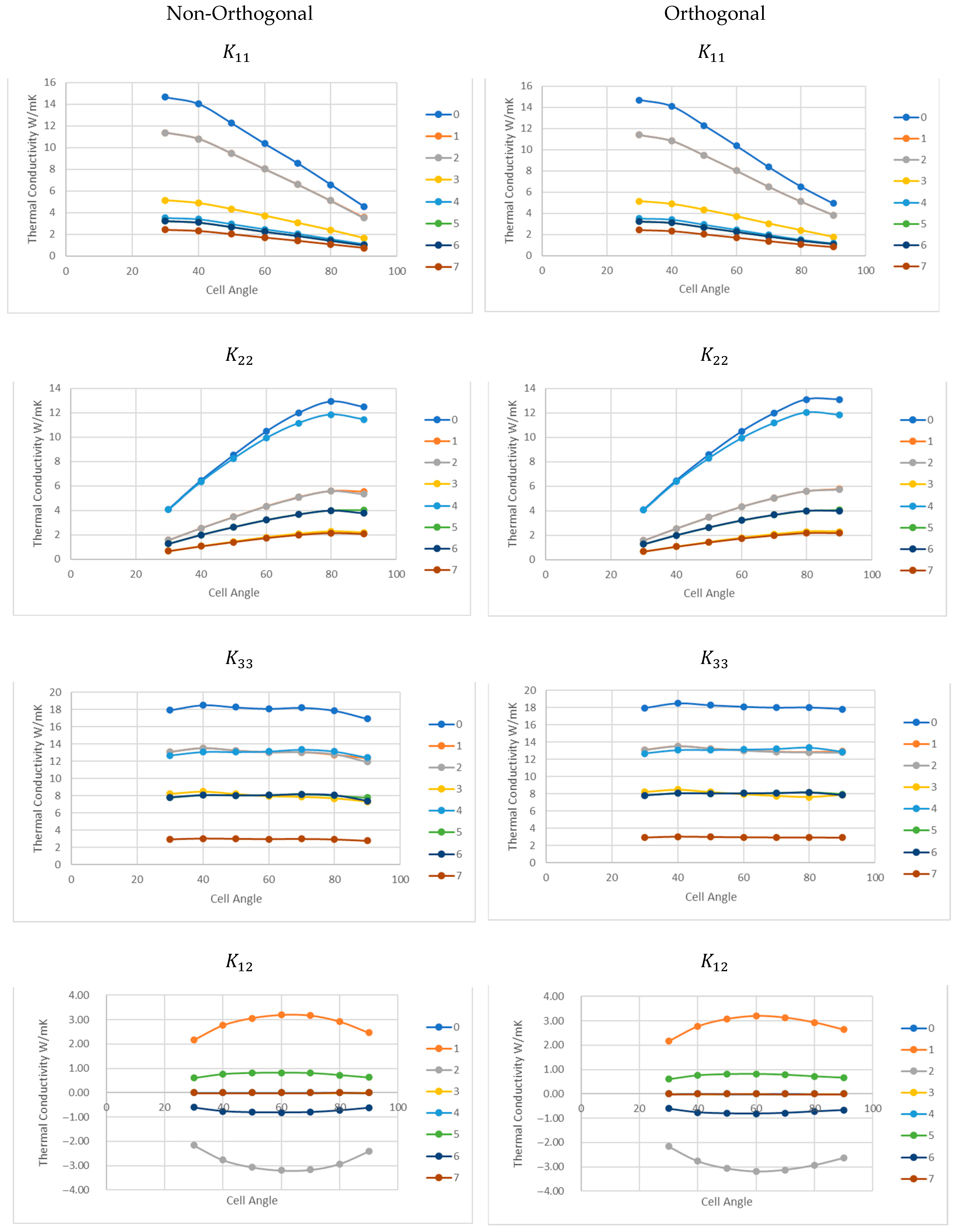
4.2. Variation in Thermal Conduction w.r.t Cell Angle for Multiple Material Configuration

The thermal conductivity coefficients in the x-, y-, and z-axes are shown in Figure 16. Based on this observation, the thermal conductivity coefficients in the x and y directions are inversely proportional to each other. Whereas the thermal conductivity in the z direction ($K_{33}$) remains constant due to the periodic boundary condition imposed in the out-of-plane direction. Due to the bi-material nature of some configuration, the non-diagonal term $K_{12}$ has non-zero values, which dictate that the thermal conductivity is coupled in the x and y directions.

5. Conclusions

The homogenized thermal expansion and conduction properties of 2D and 3D lattices can be performed using the discretized voxel mesh AH approach regardless of the shape of the RVE cell envelope being orthogonal or non-orthogonal. Approximating the periodicity on an imperfect voxel mesh misaligns the periodic node pairs and causes numerical errors. These numerical errors are observed for some lattices whose zero terms in off-diagonal terms are replaced with non-zero values for thermal expansion and conduction. The numerical errors observed for thermal conduction were at least three orders of magnitude smaller in comparison to the main diagonals, whereas the thermal expansion errors were at least six orders of magnitude smaller than the main components.

The numerical errors are mostly present in the voxels along the cell envelope, and the magnitude of the numerical errors is cyclically dependent on the number of divisions along an axis. Furthermore, by decreasing the size of the voxel, it is possible to reduce the numerical errors. For the bi-material hexagon lattice, it was show here that by choosing materials with different thermal expansion coefficients, it is possible to create lattices with large varying thermal expansion including negative thermal expansion coefficients.

References

1. Sigmund, O.; Torquato, S. Design of Materials with Extreme Thermal Expansion Using a Three-Phase Topology Optimization Method. J. Mech. Phys. Solids 1997, 45, 1037–1067. [Google Scholar] [CrossRef]
2. Xu, H.; Pasini, D. Structurally Efficient Three-Dimensional Metamaterials with Controllable Thermal Expansion. Sci. Rep. 2016, 6, 34924. [Google Scholar] [CrossRef]
3. Chen, J.; Xu, W.; Wei, Z.; Wei, K.; Yang, X. Stiffness Characteristics for a Series of Lightweight Mechanical Metamaterials with Programmable Thermal Expansion. Int. J. Mech. Sci. 2021, 202–203, 106527. [Google Scholar] [CrossRef]
4. Grima, J.N.; Farrugia, P.S.; Gatt, R.; Zammit, V. A System with Adjustable Positive or Negative Thermal Expansion. Proc. R. Soc. A Math. Phys. Eng. Sci. 2007, 463, 1585–1596. [Google Scholar] [CrossRef]
5. Holmén, A. Multi-Metamaterial Composites: Kelvin Cell Derivatives in Pursuit of Low Thermal Expansion and Poisson’s Ratio. Master’s Thesis, KTH, Royal Institute of Technology, Stockholm, Sweden, 2025. [Google Scholar]
6. Wang, Q.; Jackson, J.A.; Ge, Q.; Hopkins, J.B.; Spadaccini, C.M.; Fang, N.X. Lightweight Mechanical Metamaterials with Tunable Negative Thermal Expansion. Phys. Rev. Lett. 2016, 117, 175901. [Google Scholar] [CrossRef]
7. Dubey, D.; Mirhakimi, A.S.; Elbestawi, M.A. Negative Thermal Expansion Metamaterials: A Review of Design, Fabrication, and Applications. J. Manuf. Mater. Process. 2024, 8, 40. [Google Scholar] [CrossRef]
8. Ni, X.; Guo, X.; Li, J.; Huang, Y.; Zhang, Y.; Rogers, J.A. 2D Mechanical Metamaterials with Widely Tunable Unusual Modes of Thermal Expansion. Adv. Mater. 2019, 31, e1905405. [Google Scholar] [CrossRef]
9. Askar, A.; Cakmak, A.S.S. A Structural Model of a Micropolar Continuum. Int. J. Eng. Sci. 1968, 6, 583–589. [Google Scholar] [CrossRef]
10. Chen, J.Y.; Huang, Y.; Ortiz, M. Fracture Analysis of Cellular Materials: A Strain Gradient Model. J. Mech. Phys. Solids 1998, 46, 789–828. [Google Scholar] [CrossRef]
11. Bažant, Z.P.; Christensen, M. Analogy between Micropolar Continuum and Grid Frameworks under Initial Stress. Int. J. Solids Struct. 1972, 8, 327–346. [Google Scholar] [CrossRef]
12. Kumar, R.S.; McDowell, D.L. Generalized Continuum Modeling of 2-D Periodic Cellular Solids. Int. J. Solids Struct. 2004, 41, 7399–7422. [Google Scholar] [CrossRef]
13. van Tuijl, R.A.; Remmers, J.J.C.; Geers, M.G.D. Multi-Dimensional Wavelet Reduction for the Homogenisation of Microstructures. Comput. Methods Appl. Mech. Eng. 2019, 359, 112652. [Google Scholar] [CrossRef]
14. Vigliotti, A.; Pasini, D. Mechanical Properties of Hierarchical Lattices. Mech. Mater. 2013, 62, 32–43. [Google Scholar] [CrossRef]
15. Hutchinson, R.G.; Fleck, N.A. The Structural Performance of the Periodic Truss. J. Mech. Phys. Solids 2006, 54, 756–782. [Google Scholar] [CrossRef]
16. Elsayed, M.S.A.; Pasini, D. Analysis of the Elastostatic Specific Stiffness of 2D Stretching-Dominated Lattice Materials. Mech. Mater. 2010, 42, 709–725. [Google Scholar] [CrossRef]
17. Vigliotti, A.; Pasini, D. Linear Multiscale Analysis and Finite Element Validation of Stretching and Bending Dominated Lattice Materials. Mech. Mater. 2012, 46, 57–68. [Google Scholar] [CrossRef]
18. Xu, S.; Zhang, W. Energy-Based Homogenization Method for Lattice Structures with Generalized Periodicity. Comput. Struct. 2024, 302, 107478. [Google Scholar] [CrossRef]
19. Yu, B.; Xu, Z.; Mu, R.; Wang, A.; Zhao, H. Design of Large-Scale Space Lattice Structure with Near-Zero Thermal Expansion Metamaterials. Aerospace 2023, 10, 294. [Google Scholar] [CrossRef]
20. Florence, C.; Sab, K. A Rigorous Homogenization Method for the Determination of the Overall Ultimate Strength of Periodic Discrete Media and an Application to General Hexagonal Lattices of Beams. Eur. J. Mech. A/Solids 2006, 25, 72–97. [Google Scholar] [CrossRef]
21. Assidi, M.; Dos Reis, F.; Ganghoffer, J.-F. Equivalent Mechanical Properties of Biological Membranes from Lattice Homogenization. J. Mech. Behav. Biomed. Mater. 2011, 4, 1833–1845. [Google Scholar] [CrossRef]
22. Dos Reis, F.; Ganghoffer, J.F. Equivalent Mechanical Properties of Auxetic Lattices from Discrete Homogenization. Comput. Mater. Sci. 2012, 51, 314–321. [Google Scholar] [CrossRef]
23. Wicht, D.; Schneider, M.; Böhlke, T. Computing the Effective Response of Heterogeneous Materials with Thermomechanically Coupled Constituents by an Implicit Fast Fourier Transform-Based Approach. Int. J. Numer. Methods Eng. 2020, 122, 1307–1332. [Google Scholar] [CrossRef]
24. Lu, X.; Fu, X.; Lu, J.; Sun, R.; Xu, J.; Yan, C.; Wong, C.P. Numerical Homogenization of Thermal Conductivity of Particle-Filled Thermal Interface Material by Fast Fourier Transform Method. Nanotechnology 2021, 32, 12. [Google Scholar] [CrossRef]
25. To, Q.D.; Bonnet, G. FFT Based Numerical Homogenization Method for Porous Conductive Materials. Comput. Methods Appl. Mech. Eng. 2020, 368, 113160. [Google Scholar] [CrossRef]
26. Lages, E.N.; Pereira, S.; Marques, C. Thermoelastic Homogenization of Periodic Composites Using an Eigenstrain-Based Micromechanical Model. Appl. Math. Model. 2020, 85, 1–18. [Google Scholar] [CrossRef]
27. Schneider, M.; Merkert, D.; Kabel, M. FFT-Based Homogenization for Microstructures Discretized by Linear Hexahedral Elements. Int. J. Numer. Methods Eng. 2017, 109, 1461–1489. [Google Scholar] [CrossRef]
28. Hassani, B.; Hinton, E. A Review of Homogenization and Topology Optimization I—Homogenization Theory for Media with Periodic Structure. Comput. Struct. 1998, 69, 707–717. [Google Scholar] [CrossRef]
29. Hollister, S.J.; Kikuehi, N. A Comparison of Homogenization and Standard Mechanics Analyses for Periodic Porous Composites. Comput. Mech. 1992, 10, 73–95. [Google Scholar] [CrossRef]
30. Guedes, J.J.M.J.; Kikuchi, N. Preprocessing and Postprocessing for Materials Based on the Homogenization Method with Adaptive Finite Element Methods. Comput. Methods Appl. Mech. Eng. 1990, 83, 143–198. [Google Scholar] [CrossRef]
31. Andreassen, E.; Andreasen, C.S. How to Determine Composite Material Properties Using Numerical Homogenization. Comput. Mater. Sci. 2014, 83, 488–495. [Google Scholar] [CrossRef]
32. Dong, G.; Tang, Y.; Zhao, Y.F. A 149 Line Homogenization Code for Three-Dimensional Cellular Materials Written in MATLAB. J. Eng. Mater. Technol. Trans. ASME 2019, 141, 011005. [Google Scholar] [CrossRef]
33. Liu, S.; Zhang, Y. Multi-Scale Analysis Method for Thermal Conductivity of Porous Material with Radiation. Multidiscip. Model. Mater. Struct. 2006, 2, 327–344. [Google Scholar] [CrossRef]
34. Hill, R. A Self-Consistent Mechanics of Composite Materials. J. Mech. Phys. Solids 1965, 13, 213–222. [Google Scholar] [CrossRef]
35. Chou, T.-W.; Nomura, S.; Taya, M. A Self-Consistent Approach to the Elastic Stiffness of Short-Fiber Composites. J. Compos. Mater. 1980, 14, 178–188. [Google Scholar] [CrossRef]
36. Mori, T.; Tanaka, K. Average Stress in Matrix and Average Elastic Energy of Materials with Misfitting Inclusions. Acta Metall. 1973, 21, 571–574. [Google Scholar] [CrossRef]
37. Dasgupta, A.; Agarwal, R.K.; Bhandarkar, S.M. Three-Dimensional Modeling of Woven-Fabric Composites for Effective Thermo-Mechanical and Thermal Properties. Compos. Sci. Technol. 1996, 56, 209–223. [Google Scholar] [CrossRef]
38. Zhai, H.; Wu, Q.; Yoshikawa, N.; Xiong, K.; Chen, C. Space-Time Asymptotic Expansion Method for Transient Thermal Conduction in the Periodic Composite with Temperature-Dependent Thermal Properties. Comput. Mater. Sci. 2021, 194, 110470. [Google Scholar] [CrossRef]
39. Dasgupta, A.; Agarwal, R.K. Orthotropic Thermal Conductivity of Plain-Weave Fabric Composites Using a Homogenization Technique. J. Compos. Mater. 1992, 26, 2736–2758. [Google Scholar] [CrossRef]
40. Bowles, D.E.; Tompkins, S.S. Prediction of Coefficients of Thermal Expansion for Unidirectional Composites. J. Compos. Mater. 1989, 23, 370–388. [Google Scholar] [CrossRef]
41. Berger, H.; Gabbert, U.; Köppe, H.; Rodriguez-Ramos, R.; Bravo-Castillero, J.; Guinovart-Diaz, R.; Otero, J.A.; Maugin, G.A. Finite Element and Asymptotic Homogenization Methods Applied to Smart Composite Materials. Comput. Mech. 2003, 33, 61–67. [Google Scholar] [CrossRef]
42. Mirabolghasemi, A. Thermal Conductivity of Architected Cellular Metamaterials. Master’s Thesis, McGill University, Montreal, QC, Canada, 2018. [Google Scholar]
43. El Moumen, A.; Kanit, T.; Imad, A.; El Minor, H. Computational Thermal Conductivity in Porous Materials Using Homogenization Techniques: Numerical and Statistical Approaches. Comput. Mater. Sci. 2015, 97, 148–158. [Google Scholar] [CrossRef]
44. Kalamkarov, A.L.; Andrianov, I.V.; Danishevs’kyy, V.V. Asymptotic Homogenization of Composite Materials and Structures. Appl. Mech. Rev. 2009, 62, 030802. [Google Scholar] [CrossRef]
45. Masoumi, E.; Abad, K.; Khanoki, S.A.; Pasini, D. Fatigue Design of Lattice Materials via Computational Mechanics: Application to Lattices with Smooth Transitions in Cell Geometry. Int. J. Fatigue 2012, 47, 126–136. [Google Scholar] [CrossRef]
46. Cheng, G.D.; Cai, Y.W.; Xu, L. Novel Implementation of Homogenization Method to Predict Effective Properties of Periodic Materials. Acta Mech. Sin./Lixue Xuebao 2013, 29, 550–556. [Google Scholar] [CrossRef]
47. Liu, P.; Liu, A.; Peng, H.; Tian, L.; Liu, J.; Lu, L. Mechanical Property Profiles of Microstructures via Asymptotic Homogenization. Comput. Graph. 2021, 100, 106–115. [Google Scholar] [CrossRef]
48. Arabnejad, S.; Pasini, D. Mechanical Properties of Lattice Materials via Asymptotic Homogenization and Comparison with Alternative Homogenization Methods. Int. J. Mech. Sci. 2013, 77, 249–262. [Google Scholar] [CrossRef]
49. Peng, X.; Cao, J. A Dual Homogenization and Finite Element Approach for Material Characterization of Textile Composites. Compos. Part B Eng. 2002, 33, 45–56. [Google Scholar] [CrossRef]
50. Guinovart-Daz, R.; Rodrguez-Ramos, R.; Bravo-Castillero, J.; Sabina, F.J.; Dario Santiago, R.; Martinez Rosado, R. Asymptotic Analysis of Linear Thermoelastic Properties of Fiber Composites. J. Thermoplast. Compos. Mater. 2007, 20, 389–410. [Google Scholar] [CrossRef]
51. Visrolia, A.; Meo, M. Multiscale Damage Modelling of 3D Weave Composite by Asymptotic Homogenisation. Compos. Struct. 2013, 95, 105–113. [Google Scholar] [CrossRef]
52. Takano, N.; Zako, M.; Kubo, F.; Kimura, K. Microstructure-Based Stress Analysis and Evaluation for Porous Ceramics by Homogenization Method with Digital Image-Based Modeling. Int. J. Solids Struct. 2003, 40, 1225–1242. [Google Scholar] [CrossRef]
53. Dong, K.; Liu, K.; Zhang, Q.; Gu, B.; Sun, B. Experimental and Numerical Analyses on the Thermal Conductive Behaviors of Carbon Fiber/Epoxy Plain Woven Composites. Int. J. Heat Mass Transf. 2016, 102, 501–517. [Google Scholar] [CrossRef]
54. Hashin, Z. Analysis of Composite Materials—A Survey. J. Appl. Mech. 1983, 50, 481–505. [Google Scholar] [CrossRef]
55. Rosen, B.W.; Hashin, Z. Effective Thermal Expansion Coefficients and Specific Heats of Composite Materials. Int. J. Eng. Sci. 1970, 8, 157–173. [Google Scholar] [CrossRef]
56. Chamis, C.C.; Sendeckyj, G.P. Critique on Theories Predicting Thermoelastic Properties of Fibrous Composites. J. Compos. Mater. 1968, 2, 332–358. [Google Scholar] [CrossRef]
57. Mirabolghasemi, A.; Akbarzadeh, A.H.; Rodrigue, D.; Therriault, D. Thermal Conductivity of Architected Cellular Metamaterials. Acta Mater. 2019, 174, 61–80. [Google Scholar] [CrossRef]
58. Zhang, Y.; Shang, S.; Liu, S. A Novel Implementation Algorithm of Asymptotic Homogenization for Predicting the Effective Coefficient of Thermal Expansion of Periodic Composite Materials. Acta Mech. Sin./Lixue Xuebao 2017, 33, 368–381. [Google Scholar] [CrossRef]
59. Material Designer User’s Guide. Available online: https://ansyshelp.ansys.com/account/secured?returnurl=/Views/Secured/corp/v194/acp_md/acp_md.html (accessed on 16 December 2020).
60. Hassani, B.; Hinton, E. A Review of Homogenization and Topology Opimization II—Analytical and Numerical Solution of Homogenization Equations. Comput. Struct. 1998, 69, 719–738. [Google Scholar] [CrossRef]
61. Hassani, B.; Hinton, E. A Review of Homogenization and Topology Optimization III—Topology Optimization Using Optimality Criteria. Comput. Structures 1998, 69, 739–756. [Google Scholar] [CrossRef]
62. Rajakareyar, P. Thermo-Elastic Mechanics of Morphing Lattice Structures with Applications in Shape Optimization of BLI Engine Intakes. Master’s Thesis, Carleton University, Ottawa, ON, Canada, 2023. [Google Scholar]
63. Rajakareyar, P.; ElSayed, M.S.A.; Abo El Ella, H.; Matida, E. Effective Mechanical Properties of Periodic Cellular Solids with Generic Bravais Lattice Symmetry via Asymptotic Homogenization. Materials 2023, 16, 7562. [Google Scholar] [CrossRef] [PubMed]
64. Virtanen, P.; Gommers, R.; Oliphant, T.E.; Haberland, M.; Reddy, T.; Cournapeau, D.; Burovski, E.; Peterson, P.; Weckesser, W.; Bright, J.; et al. SciPy 1.0: Fundamental Algorithms for Scientific Computing in Python. Nat. Methods 2020, 17, 261–272. [Google Scholar] [CrossRef] [PubMed]
65. Logan, D.L. A First Course in the Finite Element Method, SI ed.; Cengage Learning: Boston, MA, USA, 2016. [Google Scholar]
66. SPACEMATDB—Space Materials Database. Materials Details. Available online: https://www.spacematdb.com/spacemat/datasearch.php?name=Invar 36 (accessed on 30 July 2022).
67. Van Der Walt, S.; Colbert, S.C.; Varoquaux, G. The NumPy Array: A Structure for Efficient Numerical Computation. Comput. Sci. Eng. 2011, 13, 22–30. [Google Scholar] [CrossRef]
68. SciPy, Scipy.Spatial.CKDTree—SciPy v1.5.4 Reference Guide. 2022. Available online: https://docs.scipy.org/doc/scipy/reference/generated/scipy.spatial.cKDTree.html (accessed on 11 December 2020).
69. Hunter, J.D. Matplotlib: A 2D Graphics Environment. Comput. Sci. Eng. 2007, 9, 90–95. [Google Scholar] [CrossRef]
70. Ramachandran, P.; Varoquaux, G. Mayavi: 3D Visualization of Scientific Data. Comput. Sci. Eng. 2011, 13, 40–51. [Google Scholar] [CrossRef]
71. Gaillac, R.; Pullumbi, P.; Coudert, F.-X. ELATE: An Open-Source Online Application for Analysis and Visualization of Elastic Tensors. J. Phys. Condens. Matter 2016, 28, 275201. [Google Scholar] [CrossRef] [PubMed]
72. Kermode, J.; Pastewka, L. Matscipy/Elasticity.Py at Master · LibAtoms/Matscipy. Available online: https://github.com/libAtoms/matscipy/blob/master/matscipy/elasticity.py (accessed on 11 December 2020).
73. Hoogendoorn, E.; van Golen, K. Numpy-Indexed · PyPI. Available online: https://pypi.org/project/numpy-indexed/. (accessed on 11 December 2020).
74. Lam, S.K.; Pitrou, A.; Seibert, S. Numba: A LLVM-Based Python JIT Compiler. In Proceedings of the Second Workshop on the LLVM Compiler Infrastructure in HPC-LLVM ’15, Austin, TX, USA, 15 November 2015; pp. 1–6. [Google Scholar]
Figure 1. Iso-parametric hexahedral voxel element, with global coordinate system ( x , y , z ), local coordinate system ( ξ , ζ , η ) and voxel edges aligned with global coordinate system with lengths ( l x , l y , l z ) respectively.
Symmetry 17 01197 g001
Figure 2. AH workflow for calculating thermal expansion and thermal conduction for arbitrary cellular geometry.
Symmetry 17 01197 g002
Figure 3. (a) Hexagonal lattice with various cell envelope characteristics. Periodic bases are indicated with red and green arrows for the three proposed envelopes. (b) Visualization illustrates the 2D Open Hexagon with the RVE’s envelope, voxels, and periodic basis. The shape of voxels is not to scale.
Symmetry 17 01197 g003
Figure 4. Cell envelope definition for filtering voxels with zero and non-zero volume. Red voxel centers are considered to be inside the cell envelope, whereas blue colored voxel centers are outside the cell envelope based on the direction of the cell envelope normal (orange arrow).
Symmetry 17 01197 g004
Figure 5. Identification of a periodic node pair for node i situated at ( x 1 i , x 2 i ) alongside its periodic counterpart i at N i Y i , and the search radius R (green arrow and circle), necessary for locating the approximate periodic node pair owing to the discrepancy between the voxel element basis and the RVE’s periodic basis. This search radius can be utilized with a KD-Tree method [64] to query the nearest location. Residuals G 1 and G 2 are shown assuming point s being chosen as the periodic node pair.
Symmetry 17 01197 g005
Figure 6. (a) Hexagon cell angle definition. (b) Material distribution and (c) bisection planes based on truss orientation. The individual truss definition in (b) is shown in multiple colors. For the closed hexagon, the truss ID (black font) is shown with its periodic Truss ID (red font). The full closed hexagon lattice’s RVE is marked in solid black line. The closed hexagon’s periodic cell envelope is shown as dashed black line, whereas the orthogonal hexagon’s cell envelope is shown as a dashed red line. (c) Shows how individual trusses in the open and closed hexagon RVE is split using the bisector planes (black solid lines).
Symmetry 17 01197 g006
Figure 7. Geometry of uni-directional fiber composite and its material properties.
Symmetry 17 01197 g007
Figure 8. Comparison of thermal expansion and thermal conduction results from homogenization framework and ANSYS for the unidirectional composite. (a) Thermal conductivity properties for UD Composite with varying fiber density; (b) Thermal expansion properties for UD composite with varying fiber density.
Symmetry 17 01197 g008
Figure 9. Thermal conductivity anisotropy for (a) UD composite and (b) 2D square made from copper and steel.
Symmetry 17 01197 g009
Figure 10. Variation in thermal conduction based on the discretization of closed hexagon lattice. (a) Shows the main terms of the thermal conductivity matrix as it varies with number of voxel divisions. (b) Shows the off-diagonal terms of the thermal conductivity matrix.
Symmetry 17 01197 g010
Figure 11. Variation in thermal expansion coefficients based on the discretization of closed hexagon lattice.
Symmetry 17 01197 g011
Figure 12. Visualization of the influence of the voxel towards the Thermal Conduction matrix for (a) closed hexagon and (b) open hexagon. The off-diagonal contribution towards the zero term, which contributes to the numerical, is also shown.
Symmetry 17 01197 g012
Figure 13. Visualization of the periodicity node pairs. Each line of a random color represents a coupling of the degrees of freedom for that node pair. The periodic basis has been highlighted as thick green lines. (a) Closed hexagon with larger mesh (b) Closed hexagon with fine mesh.
Symmetry 17 01197 g013
Figure 14. Voxelized orthogonal hexagon (top) and closed hexagon (bottom) lattice shown for cell angles 30°, 60° and 80°. Individual trusses of the closed hexagon lattice has been colored differently.
Symmetry 17 01197 g014
Figure 15. Comparison of large non-zero thermal expansion coefficients for the orthogonal and the non-orthogonal hexagon lattice.
Symmetry 17 01197 g015
Figure 16. Comparison of large non-zero thermal conduction coefficients for the orthogonal and the non-orthogonal hexagon lattice. Some of the discrepancies in the results were mostly due to the voxel discretization causing variation in the volume fraction.
Symmetry 17 01197 g016