DFAN: Single Image Super-Resolution Using Stationary Wavelet-Based Dual Frequency Adaptation Network

Abstract

Single image super-resolution is the inverse problem of reconstructing a high-resolution image from its low-resolution counterpart. Although recent Transformer-based architectures leverage global context integration to improve reconstruction quality, they often overlook frequency-specific characteristics, resulting in the loss of high-frequency information. To address this limitation, we propose the Dual Frequency Adaptive Network (DFAN). DFAN first decomposes the input into low- and high-frequency components via Stationary Wavelet Transform. In the low-frequency branch, Swin Transformer layers restore global structures and color consistency. In contrast, the high-frequency branch features a dedicated module that combines Directional Convolution with Residual Dense Blocks, precisely reinforcing edges and textures. A frequency fusion module then adaptively merges these complementary features using depthwise and pointwise convolutions, achieving a balanced reconstruction. During training, we introduce a frequency-aware multi-term loss alongside the standard pixel-wise loss to explicitly encourage high-frequency preservation. Extensive experiments on the Set5, Set14, BSD100, Urban100, and Manga109 benchmarks show that DFAN achieves up to +0.64 dBpeak signal-to-noise ratio, +0.01 structural similarity index measure, and −0.01learned perceptual image patch similarity over the strongest frequency-domain baselines, while also delivering visibly sharper textures and cleaner edges. By unifying spatial and frequency-domain advantages, DFAN effectively mitigates high-frequency degradation and enhances SISR performance.

1. Introduction

Single-image super-resolution (SISR) seeks to reconstruct a high-resolution (HR) image $I_{HR}$ from a single low-resolution (LR) observation $I_{LR}$. Because the missing high-frequency details must be inferred from only one input, the task is intrinsically ill posed [1,2]. By restoring fine structural and textural information lost owing to limited sensor optics or storage constraints, SISR enhances the accuracy of downstream computer-vision pipelines [3]. Thanks to these benefits, SISR is now routinely adopted as a generic pre-processing step in many vision systems, where it helps lift performance ceilings in tasks such as object detection, semantic segmentation, and multi-object tracking [4].

To improve SISR performance, researchers have refined strategies along three main axes: network architecture design, loss-function engineering, and inference-phase enhancement. First, in terms of architecture, residual CNNs that extend depth and width (e.g., VDSR and EDSR [5,6] following SRCNN [7]), networks that combine channel- and spatial-attention modules (e.g., RDN and RCAN [8,9]), and Transformer-based models that capture long-range dependencies (e.g., SwinIR and HAT [10,11]) have successively raised the upper limits of the representative metrics PSNR and SSIM [12,13]. Second, for the learning objective, studies have introduced perceptual loss in VGG feature space [14], GAN-based adversarial loss [15], and frequency-filter losses that emphasize edge and texture precision [16] in addition to the simple L1/L2 reconstruction error, thereby improving visual sharpness and naturalness. Third, at the inference stage, techniques such as iterative back-projection, which repeatedly refines frequency- and scale-specific reconstructions [17], multi-scale ensembling [18], unsupervised domain adaptation that mimics real-world degradations [19], and test-time augmentation (TTA) [20] further enhance the restoration quality. Nevertheless, most of these approaches still focus on extending spatial-domain correlations or designing statistical losses and do not fundamentally solve the high-frequency preservation problem that determines actual restoration quality.

Image signals can be analyzed in the frequency domain, where they are represented by periodic bases instead of spatial coordinates [21]. In this domain, low-frequency components capture gradual variations in global illumination and chroma. In contrast, high-frequency components describe delicate structures in which pixel values change abruptly, such as edges, contours, and textures [22]. Because conventional down-sampling and compression preferentially discard high-frequency content with large spectral amplitudes [23], restoring the missing high frequencies is the central challenge of SISR. High-frequency information directly affects not only traditional pixel-wise metrics, such as PSNR and SSIM [12,13], but also perceptual quality scores, including LPIPS and the Perceptual Index [24], as well as the accuracy of subsequent tasks, including object detection, segmentation, and recognition. For instance, blurred boundaries cause detection boxes to bleed, and when delicate textures are not recovered, class-specific traits (e.g., fabric patterns or surface scratches) are diluted, leading to degraded classification and recognition performance [25]. Conversely, excessive amplification of high-frequency content can introduce artifacts such as ringing and overshoot [26], so a balanced restoration strategy across frequency bands is essential. Consequently, a SISR network must model high-frequency information in a frequency-aware manner.

Contemporary SISR research has shifted toward Transformer-based models such as SwinIR and HAT [10,11]. While these networks raise PSNR and SSIM scores [12,13] by efficiently capturing long-range dependencies, they do not explicitly exploit band-specific frequency characteristics. In window-based self-attention, local tokens are averaged within fixed patches, so high-frequency details are merged with low-frequency content in the same token representation, which imparts an overall low-pass tendency to the reconstruction [27]. Consequently, despite their strength in global correlation modeling, these models lack structural mechanisms for selectively enhancing or preserving high-frequency components and, thus, still show limitations in recovering fine edges and textures.

In this work, we introduce a Dual-Frequency Adaptive Network (DFAN) that leverages the inherent symmetry of image frequency components to overcome the high-frequency loss seen in prior Transformer-based SISR models. The low-resolution input image $I_{LR}$ is first decomposed by a Stationary Wavelet Transform (SWT) [28] into four sub-bands, $I_{LR}\to (LL,LH,HL,HH)$, where $LL$ is the low-frequency band and $LH$, $HL$, and $HH$ are the mutually orthogonal horizontal, vertical, and diagonal high-frequency bands, respectively, thus forming a dual symmetric partition between low- and high-pass information. These components are processed in two structurally mirrored branches in the high-frequency branch; each HF band is selectively filtered by a Directional Convolution that preserves horizontal, vertical, and diagonal edge symmetry, then refined by a Residual Dense Block (RDB) to enhance textures in the low-frequency branch, and the $LL$ band is reconstructed by a Swin Transformer layer to restore global structure. The resulting feature maps are fused by a depthwise–pointwise Feature Fusion Module that adaptively balances the two pathways while maintaining channel- and spatial-level symmetry. During training, a frequency-aware multi-term loss combines conventional reconstruction error with frequency-domain penalties, explicitly guiding the network to retain HF energy. By unifying spatial and frequency advantages and by preserving symmetrical consistency from decomposition through PixelShuffle reconstruction, DFAN fundamentally mitigates high-frequency attenuation and delivers performance superior to existing methods.

The contributions of the proposed method in this study are as follows:

• Frequency-decomposition dual pipeline: The input image is separated into low- and high-frequency bands by SWT and processed in parallel, thereby combining the strengths of both spatial and frequency domains.
• Directional high-frequency module and fusion module: Sub-band-specific Directional Convolution followed by RDB amplifies and refines high-frequency details, which are then adaptively merged with the low-frequency global context in the Fusion Module to recover fine textures.
• Frequency-aware multi-loss function: A high-frequency loss term is added to the conventional reconstruction loss, forcing the network to learn the importance of high-frequency information explicitly.
• Superior super-resolution performance: The proposed design consistently surpasses state-of-the-art frequency-domain SISR methods not only in PSNR and SSIM but also in perceptual quality metrics such as LPIPS.

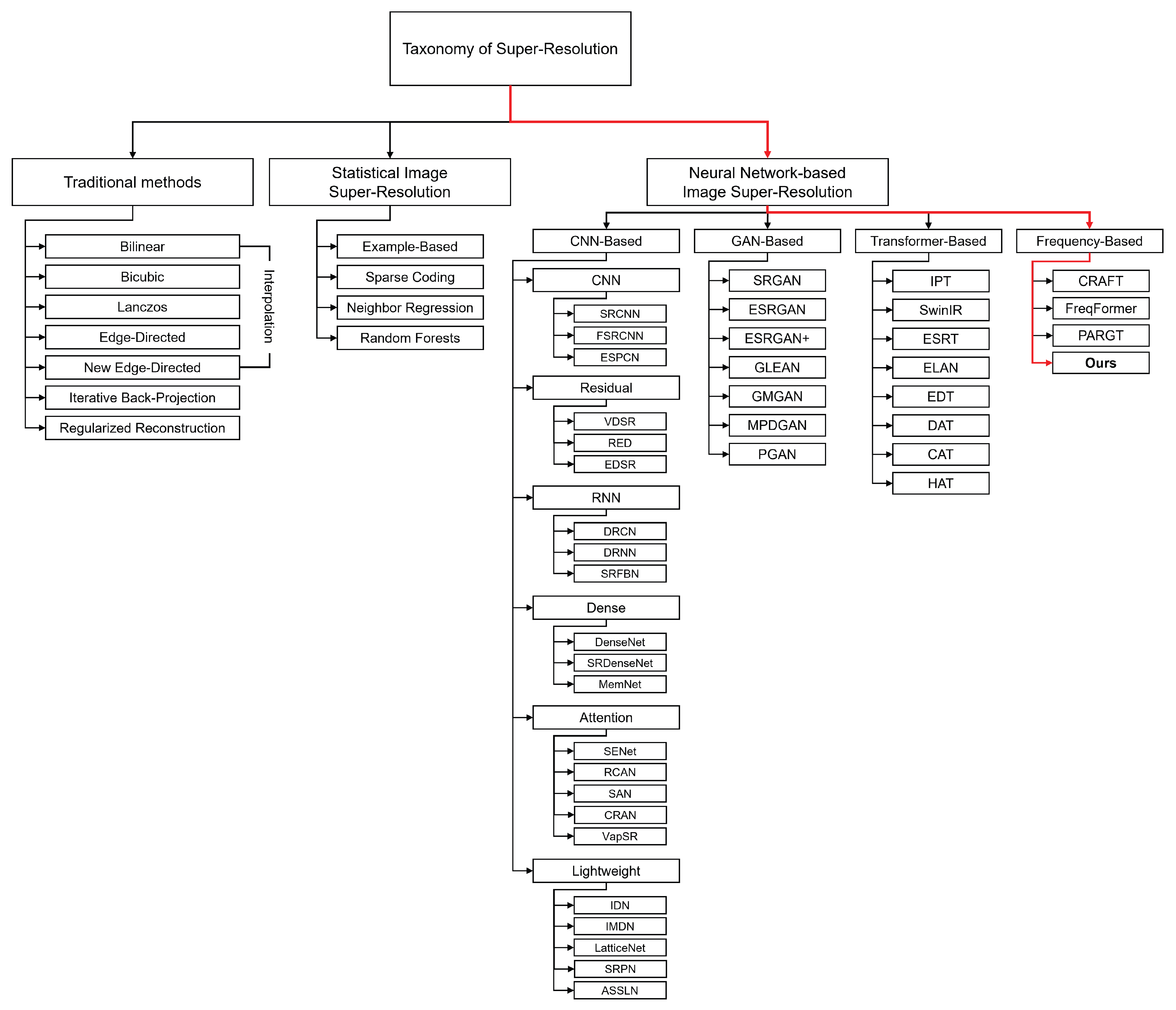
The remainder of this paper is organized as follows. Section 2 surveys the evolution of super-resolution techniques, comparing the strengths and weaknesses of traditional, statistical image super-resolution, and neural network-based image super-resolution approaches. Section 3 provides a detailed description of the proposed Dual-Frequency Adaptive Network (DFAN), including its frequency-decomposition dual pipeline, directional high-frequency module, frequency–spatial fusion scheme, and frequency-aware loss function. Section 4 outlines the experimental setup, evaluation metrics, and both quantitative and qualitative results on public benchmark datasets, demonstrating that DFAN surpasses the latest methods. Finally, Section 5 summarizes the findings, discusses limitations, and outlines directions for future work.

2. Related Work

Research on super-resolution can be broadly divided, according to its historical development, into traditional methods, statistical image super-resolution methods, and neural network-based image super-resolution methods. Figure 1 shows a taxonomy of super-resolution.

2.1. Traditional Methods

Traditional approaches begin with interpolation or reconstruction techniques that assume intra-image pixel continuity without relying on multi-frame information. Representative linear interpolation schemes such as bilinear, bicubic, and Lanczos filters [29,30,31] estimate new pixel values by computing a kernel-weighted average of neighboring pixels, while edge-directed methods such as Edge-Directed Interpolation (EDI) and New Edge-Directed Interpolation (NEDI) [32,33] improve boundary preservation by incorporating local gradient orientation. In addition, Iterative Back-Projection (IBP) and regularized reconstruction methods [34,35] repeatedly invert the low-resolution observation model to recover a high-resolution image. These classical techniques, nevertheless, have notable limitations: they reproduce low-frequency content more effectively than high-frequency details, their performance degrades sharply when the blur, noise, or down-sampling model is inaccurate, and, lacking data-driven learning, they adapt poorly to diverse content and degradation types [36,37,38]. Such constraints have underscored the need for subsequent machine learning and deep learning approaches.

2.2. Statistical Image Super-Resolution Methods

Machine learning approaches were introduced to overcome the limitations of interpolation- and reconstruction-based methods by learning the correspondence between low-resolution (LR) and high-resolution (HR) patches. Freeman et al. [39] linked a pre-built LR–HR patch dictionary with a Markov random field and combined HR patches under boundary-consistency constraints to synthesize the high-resolution image. Yang et al. [40] learned a coupled LR–HR dictionary pair that shares a common sparse code; the sparse coefficients obtained from an LR patch were projected onto the HR dictionary to recover fine structures. Both techniques, nevertheless, required either exhaustive search or L1 optimization at inference time, resulting in heavy computation. To alleviate this burden, Timofte et al. [41] proposed Anchored Neighborhood Regression (ANR), which clusters dictionary patches into anchor centroids and pre-computes a linear regressor for each cluster, enabling real-time inference. Building on this idea, Schulter et al. [42] introduced Super-Resolution Forests, a decision-tree random forest model that performs nonlinear local regression at each split node. Meanwhile, Li et al. [43] augmented the framework with gradient and color features to increase the representational power of leaf-node regression. Although these machine learning methods surpass classical techniques in learning-inference efficiency and resolution generalization, they still lack global contextual information owing to their local patch assumption and remain sensitive to the size of the dictionary and the number of clusters.

2.3. Neural Network-Based Image Super-Resolution Methods

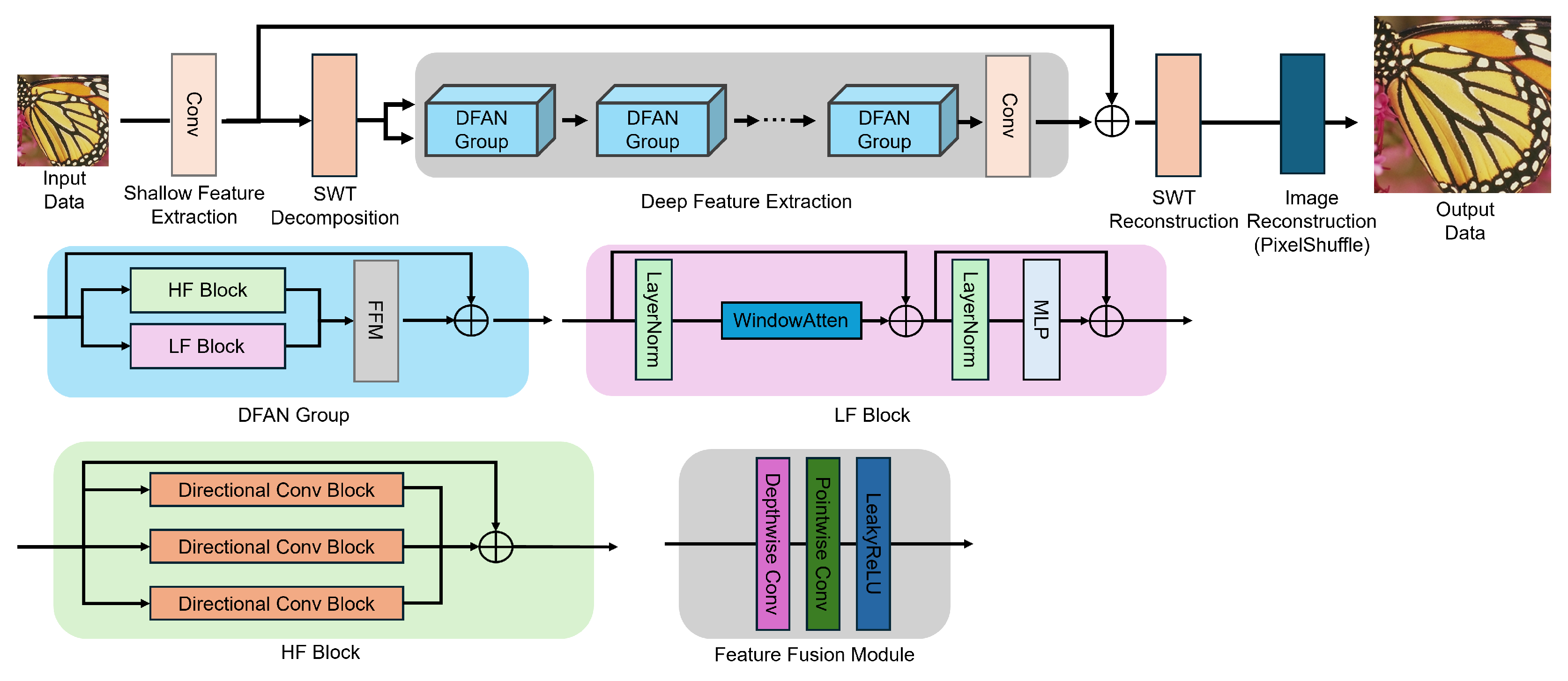
CNN-based super-resolution research has progressed through six distinct branches, each defined by its network structure. Dong et al. [7] proposed SRCNN, a model that directly regresses low-resolution (LR) patches to high-resolution (HR) patches in an end-to-end fashion, demonstrating the feasibility of learning-based super-resolution (SR). Dong et al. [44] later introduced FSRCNN, which removed pre-upsampling and performed the computations and deconvolution in the LR space, greatly accelerating inference, while Shi et al. [45] developed ESPCN, achieving real-time video SR with sub-pixel convolution. In the residual branch, Kim et al. [5] presented VDSR, attaining high-quality restoration with a 20-layer residual network, and Mao et al. [46] proposed RED, which mitigated low-frequency loss through symmetric skip connections. Lim et al. [6] introduced EDSR, eliminating batch normalization and widening the blocks, thereby leading benchmark performance. The recurrent branch improves efficiency by parameter sharing: Kim et al. [47] proposed DRCN, which recursively applied a single filter set dozens of times, Tai et al. [48] introduced DRRN, stacking residuals inside recursive blocks to strengthen information flow, and Li et al. [49] developed SRFBN, refining LR and HR features iteratively via a feedback loop. The dense branch maximizes feature reuse. Huang et al. [50] introduced DenseNet, whose concept was extended to SR by Tong et al. [51] as SRDenseNet, suppressing gradient vanishing through full layer connectivity, while Tai et al. [52] proposed MemNet, introducing long- and short-term memory blocks for precise restoration. The attention branch dynamically modulates the importance of channels and spatial locations. Hu et al. [53] introduced SENet, the first to apply channel attention, Zhang et al. [9] proposed RCAN, extending channel attention to residual blocks, Dai et al. [54] developed SAN, enhancing texture depiction with second-order attention, Zhang et al. [55] proposed CRAN, improving performance through context reasoning attention, and Zhou et al. [56] introduced VapSR, which uses vast-receptive-field attention for better efficiency. Finally, the lightweight branch targets mobile and embedded environments: Hui et al. [57,58] proposed IDN and IMDN, reducing parameters via information distillation, Luo et al. [59] introduced LatticeNet, minimizing computation with lattice blocks, and Zhang et al. [60,61] proposed SRPN and ASSLN, achieving further model compression through structure-regularized pruning and aligned sparsity learning. Although these CNN-based studies have continuously advanced depth, density, attention, and efficiency, their limited global receptive fields have motivated a recent shift toward Transformer-based designs.

Generative-adversarial approaches introduce a generator–discriminator game to overcome the perceptual-quality ceiling. Ledig et al. [14] proposed SRGAN, which first demonstrated photo-realistic HR texture synthesis by combining a VGG-based perceptual loss with an adversarial loss. Wang et al. [62] presented ESRGAN, strengthening sharp edges and fine details by replacing batch normalization with a residual-in-residual dense block (RRDB) and employing a relativistic GAN discriminator, whereas Rakotonirina et al. [63] introduced ESRGAN+, further improving visual quality and stability through dynamic feature fusion and a refined training strategy. Chan et al. [64] proposed GLEAN, which leverages a StyleGAN2 latent bank and multi-scale latent-space mapping to recover high-resolution details, achieving robust performance under complex degradations. Zhu et al. [65] introduced GMGAN, adding a quality-focused loss to alleviate mode collapse and balance fine textures against structural fidelity. Kuznedelev et al. [66] developed MPDGAN, which combines a patch discriminator with multi-perceptual losses, delivering lightweight yet high-quality super-resolution (SR) while contrasting the strengths and weaknesses of generative adversarial networks (GANs) versus diffusion models. Finally, Mahapatra et al. [67] proposed PGAN, integrating progressive generation and attention mechanisms to specialize in restoring fine tissue details in medical images. Although these GAN-based studies have markedly improved perceptual realism, issues such as training instability, ringing artifacts, and excessive high-frequency amplification persist, underscoring the need for frequency-aware regularization and hybrid designs with Transformers.

Transformer-based methods have introduced long-range dependency modeling and strong pre-training capacity into low-level restoration, thereby broadening the performance horizon. Chen et al. [68] proposed IPT, combining large-scale ImageNet pre-training with task-specific fine-tuning and demonstrating versatility across diverse restoration tasks. Liang et al. [10] introduced SwinIR, which fuses shifted-window self-attention with residual–skip connections to achieve both computational efficiency and high quality. In contrast, Lu et al. [69] proposed ESRT, placing a CNN front-end in parallel with a Transformer to balance local detail and global context. Zhang et al. [70] presented ELAN, which maximizes the receptive field with stripe-pattern long-range attention while reducing the parameter count. Li et al. [71] introduced EDT, offering an efficient pre-training strategy and a lightweight decoder that lowers inference latency for low-level vision tasks. Chen et al. [72] proposed DAT, which boosts performance by dual-aggregating local and global information. Subsequently, Chen et al. [73] introduced CAT, enhancing adaptive feature exchange between the two paths through a cross-aggregation structure. Finally, Chen et al. [11] developed HAT, extending active pixels beyond window boundaries to compensate for information loss caused by inaccurate window partitioning. Although these works continually improve PSNR and SSIM through the Transformer’s global perception, their insufficient discrimination of frequency bands still leaves room for improvement in fine, high-frequency details.

More recently, frequency-domain approaches have sought to incorporate explicit spectral priors into the super-resolution pipeline. Li et al. [36] introduced CRAFT, a Feature-Modulation Transformer that injects a learnable high-frequency prior into cross-refinement layers, boosting texture fidelity without sacrificing global coherence. Dai et al. [37] proposed FreqFormer, which performs discrete cosine–domain splitting and frequency-selective gating inside each attention block, thereby aligning spectral energy across scales and achieving competitive perceptual quality. Wang et al. [38] developed PARGT, a pixel-aware recursive generative transformer that adaptively re-weights sub-band responses to restore fine details while keeping distortion measures low. Our DFAN also belongs to this frequency-driven family, but goes further by performing stationary wavelet decomposition, deploying dedicated directional CNNs for high-frequency enhancement, and fusing the dual branches through an adaptive frequency–spatial module, which together yield state-of-the-art results.

Recent work has explored learning directly in the frequency domain. Ruan et al. [74] encode multi-axis spectral representations for medical-image segmentation, and Zhong et al. [75] detect camouflaged objects by spectral contrast. While effective in their respective domains, these models are task-specific and not designed for pixel-wise restoration, and they focus on recognition accuracy rather than balanced low-high frequency reconstruction. Consequently, they do not address the HF attenuation that dominates SISR quality. This gap motivates our Dual-Frequency Adaptive Network (DFAN), which separates, enhances, and fuses low- and high-frequency bands and is trained with an explicit frequency-aware loss.

In summary, although deep-learning advances, such as extending network depth, introducing perceptual losses, and exploiting global attention, have continually improved both quantitative and qualitative performance, a systematic framework for explicitly enhancing high-frequency components remains absent. Consequently, even the latest models still exhibit low-pass behavior in edge and texture reconstruction, failing to resolve the underutilization of high-frequency information fundamentally.

3. Proposed Method

The remainder of Section 3 is organized as follows. Section 3.1 introduces the notation, wavelet decomposition, and symbol conventions used throughout. Section 3.2 gives a top-level description of DFAN, outlining how shallow features, a stack of DFAN Groups, and the PixelShuffle head interact. Section 3.3 details the low-frequency branch based on windowed self-attention. Section 3.4 explains the high-frequency branch that combines directional convolutions with residual dense blocks for edge- and texture refinement, and describes the depthwise–pointwise mechanism that adaptively balances the two frequency pathways. Finally, Section 3.5 defines the frequency-aware training objective that couples spatial reconstruction error with band-specific frequency loss.

3.1. Preliminaries

Table 1. Notations used for describing the proposed method.

Symbol	Name	Description
$I_{LR}$	Low-Resolution Image	Input Low-Resolution Image
$I_{HR}$	High-Resolution Image	Ground-Truth HR Image
${\widehat{I}}_{HR}$	Reconstructed HR Image	Restored High-Resolution Image
$S(·)$	SWT Decomposition	Stationary Wavelet Transform Decomposition
$S^{-1}(·)$	SWT Reconstruction	Stationary Wavelet Transform Reconstruction
$Conv(·)$	Convolution	$3\times 3$ Convolution
$[·]$	concat	Combine Multiple Feature Maps
$\theta$	Network Parameters	DFAN Full Learning Parameters Set
${\mathcal{L}}_{\mathrm{spatial}}$	Spatial Loss	Pixel Reconstruction L1 Loss
${\mathcal{L}}_{\mathrm{freq}}$	Frequency Loss	Frequency Reconfiguration Loss
${\mathcal{L}}_{\mathrm{total}}$	Total Loss	${\mathcal{L}}_{\mathrm{spatial}}$ + ${\mathcal{L}}_{\mathrm{freq}}$

summarizes the notations and their meanings used to describe the proposed method. When the low-resolution input image $I_{LR}$ is passed through the Stationary Wavelet Transform operator $S(·)$, it is decomposed into a low-frequency band $LL$ and three directional high-frequency bands $LH$, $HL$, and $HH$. The low-frequency component is processed in a Swin Transformer branch $B_{LF}$, whereas the high-frequency components are handled in a branch $B_{HF}$ composed of directional convolutions and residual dense blocks. The outputs of the two branches are merged by the frequency–spatial fusion module $F_{FM}$ to produce the reconstructed image ${\widehat{I}}_{HR}$. During training, the network parameters $\mathit{\theta }$ are optimized by minimizing a total loss ${\mathcal{L}}_{\mathrm{total}}$ that combines the spatial-domain reconstruction error ${\mathcal{L}}_{\mathrm{spatial}}$ and the frequency-emphasis loss ${\mathcal{L}}_{\mathrm{freq}}$.

3.2. The Overall Structure

Figure 2 illustrates the overall pipeline of the proposed Dual-Frequency Adaptive Network. The network consists of three modules, shallow feature extraction, frequency-decomposed deep feature extraction, and image reconstruction, a structure widely adopted in prior work [9,10,11]. First, a $3\times 3$ convolution is applied to the low-resolution input $I_{LR}\in {\mathbb{R}}^{H\times W\times C_{\mathrm{in}}}$ to obtain shallow features $F_0\in {\mathbb{R}}^{H\times W\times C}$. This can be seen in Equation (1).

$$F_0=Conv\left(I_{LR}\right)$$

(1)

Next, $F_0$ is decomposed by the Stationary Wavelet Transform $S(·)$ into one low-frequency band $LL$ and three directional high-frequency bands $LH$, $HL$, and $HH$. Because the SWT is undecimated, each sub-band preserves the original spatial resolution, allowing the subsequent DFAN Groups to process low- and high-frequency information on a pixel-aligned grid. Moreover, the orthogonality of the underlying wavelet filters prevents energy leakage between the horizontal, vertical, and diagonal bands, so each branch can focus on its designated frequency content and the transform remains perfectly invertible, guaranteeing that no information is lost during decomposition and reconstruction, and A single-level decomposition is retained, as each additional level doubles the sub-band count and feature channels, increasing computation and memory almost linearly with depth. Therefore, level 1 is adopted. These sub-bands are forwarded to a series of DFAN Groups. This is evident from in Equation (2).

$$(X_{LL},X_{LH},X_{HL},X_{HH})=S\left(F_0\right)$$

(2)

Each DFAN Group comprises an HF Block, an LF Block, an FFM, and a residual connection, which jointly refine the decomposed bands in parallel. After the N consecutive DFAN Groups, their outputs are passed through a final $3\times 3$ convolution to yield the deep feature tensor

$$F_D=Conv\left(\mathrm{DFANGroup}(X_{LL},X_{LH},X_{HL},X_{HH})\right).$$

(3)

The inverse SWT then recombines the four frequency bands into a single spatial feature map,

$$F=S^{-1}\left(F_D\right),$$

(4)

and a residual addition with the shallow feature $F_0$ produces the final representation,

$$F_{\mathrm{res}}=F_0+F.$$

(5)

This staged construction prevents global representation loss while preserving both low- and high-frequency information.

Finally, the reconstruction module employs PixelShuffle-based upsampling [45] to convert the fused feature F into the high-resolution space, producing the restored image ${\widehat{I}}_{HR}$. During training, the network parameters $\mathit{\theta }$ are optimized by minimizing a total loss that combines the pixel-domain reconstruction loss ${\mathcal{L}}_{\mathrm{spatial}}$ and the frequency-domain loss ${\mathcal{L}}_{\mathrm{freq}}$, thereby jointly optimizing restoration accuracy in both spatial and frequency domains. It follows Equation (6).

$${\widehat{I}}_{HR}=\mathrm{PixelShuffle}\left(Conv\left(F_{res}\right)\right)$$

(6)

3.3. Low-Frequency Block

The Transformer-based self-attention mechanism has been reported to exhibit a low-pass effect by averaging local patch features, thereby relatively amplifying low-frequency components [76,77]. This property is advantageous for SISR, where restoring low-frequency information is crucial, and numerous studies have shown that Transformers provide richer visual representations and more stable optimization [78,79]. Leveraging this characteristic, the present work adopts the standard Swin Transformer block to construct the LF Block. The shallow feature $F_0$ is decomposed by the SWT into four sub-bands, $X_{LL},X_{LH},X_{HL},X_{HH}$, and the low-frequency component $X_{LL}$ is used as the input to the LF Block. The LF Block first applies layer normalization (LN) to the input $X_{LL}$, as shown in Equation (7).

$$X_{LL}^{\left(N\right)}=LN(+X_{LL})$$

(7)

Next, the normalized features are fed into a Window Multi-Head Self-Attention (W-MSA) module and combined with the original input through a residual connection, yielding Equation (8).

$$X_{LL}^{\left(M\right)}=\mathrm{W}\text{-}\mathrm{MSA}\left(X_{LL}^{\left(N\right)}\right)+X_{LL}$$

(8)

Finally, a second LN followed by an MLP refines the features, and another residual link produces the block output, as given in Equation (9).

$$Y_{LL}=MLP\left(LN\left(X_{LL}^{\left(M\right)}\right)\right)+X_{LL}^{\left(M\right)}$$

(9)

Equation (7) normalizes the input features, reducing inter-channel distribution shifts, Equation (8) performs window-based self-attention, thereby integrating local and global context, and Equation (9) applies a second normalization followed by an MLP, after which a residual connection is added to obtain the block output. This sequence preserves the global consistency of the low-frequency band while effectively refining the information. Window Multi-Head Self-Attention (W-MSA) first partitions the input feature map $X_{LL}^{\left(N\right)}\in {\mathbb{R}}^{H\times W\times C}$ into ${\displaystyle \frac{HW}{M^2}}$ non-overlapping local windows of size $M\times M$. Self-attention is then computed independently within each window. The operation is defined as Equation (10).

$$\mathrm{Attention}(Q,K,V)=\mathrm{SoftMax}({\displaystyle \frac{Q{K}^T}{\sqrt{d}}}+B)V$$

(10)

Here, d denotes the embedding dimension per head, and B is the relative positional encoding matrix. After computing self-attention within each window, the window outputs are reassembled into their original spatial arrangement to form the overall Window-MSA response. In this study, the input size is set to $H=W=64$, the window size to $M=16$, and the number of heads to $h=6$. Consequently, a total of ${(64/16)}^2=16$ windows are generated at a single scale, and self-attention is executed in parallel within each window. Employing such a large window size allows the model to capture context that extends beyond strictly local neighborhoods, thereby reinforcing the global consistency required for reliable low-frequency restoration.

3.4. High-Frequency Block

Figure 3 depicts the proposed HF Block. High-frequency bands carry information with abrupt pixel variations, such as edges and textures, which correlate strongly with the high-pass characteristics of convolutional neural networks (CNN) [80,81]. Accordingly, the HF Block is designed on a CNN backbone and employs the Residual Dense Block (RDB) structure [50,51,52], a proven effective core computational unit for texture reconstruction. Because the three SWT sub-bands $X_{LH},X_{HL},X_{HH}$ exhibit horizontal, vertical, and diagonal orientation, respectively, a Directional Convolution is introduced to amplify high-frequency attributes selectively. Horizontal and vertical filters are implemented with kernel shapes of $1\times 3$ and $3\times 1$, respectively, an intentional choice inspired by prior studies that show compact directional kernels are especially effective for isolating high-frequency edges and textures. The diagonal filter eliminates off-diagonal responses by multiplying its kernel weights with a diagonal mask M that activates only discriminative diagonal elements [9,54,82]. This can be seen in Equation (11).

$$X_{LH}^{\left(c\right)},X_{HL}^{\left(c\right)},X_{HH}^{\left(c\right)}=DirConv(X_{LH},X_{HL},X_{HH})$$

(11)

Immediately after the Directional Convolution, each sub-band passes through an RDB comprising three convolutional layers, where every layer concatenates its input with all previous outputs along the channel dimension, as given in Equation (12).

$$X_{LH}^{\left(R\right)},X_{HL}^{\left(R\right)},X_{HH}^{\left(R\right)}=RDB(X_{LH}^{\left(c\right)},X_{HL}^{\left(c\right)},X_{HH}^{\left(c\right)})+X_d$$

(12)

The resulting feature maps are then cross-combined via lateral connections, exchanging complementary information across sub-bands. Finally, the outputs $Y_{LH},Y_{HL},Y_{HH}$ are forwarded to the Feature Fusion Module (FFM), where they are adaptively integrated with the low-frequency branch features. The entire computation of the HF Block is expressed as Equation (13).

$$Y_{LH},Y_{HL},Y_{HH}=Con{v}_{1\times 1}[X_{LH}^{\left(R\right)},X_{HL}^{\left(R\right)},X_{HH}^{\left(R\right)}]+X_d$$

(13)

After the three directional sub-bands $Y_{LH},Y_{HL},Y_{HH}$ are individually sharpened by the HF Block’s orientation-specific convolutions and RDB refinement; they remain spectrally pure yet spatially discordant, and small phase shifts and scale misalignments persist relative to the low-frequency map $Y_{LL}$. The subsequent Feature Fusion Module (FFM) is designed to resolve these residual inconsistencies in two stages. First, the depthwise convolution $Con{v}_{dw}(3\times 3)$ applies an independent spatial filter to every channel, acting as a fine registration layer that realigns the HF responses with the corresponding LF structures while also suppressing ghosting along edges. Second, the pointwise convolution $Con{v}_{pw}(1\times 1)$ learns channel-wise mixing weights that adaptively gate the relative contributions of $Y_{LL}$ and the aggregated high-frequency tensor $Y_{HF}$, thereby equalizing spectral energy across bands before the features flow into the next DFAN Group. The LeakyReLU non-linearity that follows preserves both positive and negative high-frequency amplitudes, preventing gradient stagnation and avoiding low-pass bias. Low-frequency features $Y_{LL}$ from the LF Block and high-frequency features $Y_{LH},Y_{HL},Y_{HH}$ from the HF Block lie in disparate frequency domains simply adding them would introduce band-wise energy bias. The Feature Fusion Module (FFM) is, therefore, designed to prevent this and to achieve frequency–spatial adaptive fusion. First, the three high-frequency sub-bands are concatenated along the channel axis and linearly combined to form a single high-frequency representation $Y_{HF}$, as shown in Equation (14).

$$Y_{HF}=[Y_{LH},Y_{HL},Y_{HH}]$$

(14)

The low-frequency feature $Y_{LL}$ is then concatenated with $Y_{HF}$ along the channel dimension, yielding a composite feature $F_{\mathrm{cat}}$ that aligns information from both domains at the same spatial resolution, as given in Equation (15).

$$F_{\mathrm{cat}}=[Y_{LL},Y_{HF}]$$

(15)

A depthwise convolution $Con{v}_{\mathrm{dw}}$ is first applied to the concatenated feature tensor $F_{\mathrm{cat}},$ enabling each channel to learn an independent spatial filter and, thereby, correct residual spatial inconsistencies such as ghosting artifacts:

$$F_{\mathrm{dw}}=Con{v}_{\mathrm{dw}}\left(F_{\mathrm{cat}}\right).$$

(16)

Next, a point-wise convolution $Con{v}_{\mathrm{pw}}$ aggregates inter-channel information, and a subsequent LeakyReLU activation preserves both positive and negative high-frequency responses while avoiding gradient vanishing. This step yields the final fused sub-band features,

$$F_{LL},F_{LH},F_{HL},F_{HH}=LeakyReLU!\left(Con{v}_{\mathrm{pw}}\left(F_{\mathrm{dw}}\right)\right).$$

(17)

The module ultimately outputs the refined deep-feature set $F_{LL},F_{LH},F_{HL},F_{HH}$. After passing through the DFAN Group N times, the resulting deep feature set $F_{LL},F_{LH},F_{HL},F_{HH}$ is first processed by a $3\times 3$ convolution to suppress local noise and harmonize fine details across bands. The inverse SWT operation $S^{-1}(·)$ is then applied to restore the unified spatial-domain feature map F. Finally, F is converted to the high-resolution image ${\widehat{I}}_{HR}$ at the target scale s via a PixelShuffle-based upsampler. This step minimizes computational cost through parameter-efficient channel–spatial rearrangement while faithfully projecting the low-frequency structure and high-frequency textures, preserved by the preceding frequency separation–fusion process, into the high-resolution space.

3.5. Loss Function

DFAN is trained to minimize the total loss ${\mathcal{L}}_{\mathrm{total}}$, which combines a spatial reconstruction loss and a frequency-aware loss. All terms are defined using the L1 criterion. The spatial-domain loss is formulated as Equation (18).

$${\mathcal{L}}_{\mathrm{spatial}}=\left|\right|I_{HR}-{\widehat{I}}_{HR}\left|\right|$$

(18)

The frequency-aware loss is defined as Equation (19).

$${\mathcal{L}}_{\mathrm{d}}=\left|\right|I_{HR\left(d\right)}-{\widehat{I}}_{HR\left(d\right)}\left|\right|$$

(19)

In Equation (19), d indexes the four sub-bands $LL,LH,HL$, and $HH$. Each sub-band term is multiplied by an equal weight of 1 and then summed to yield the overall frequency loss, ensuring that this component contributes on the same numerical scale as the spatial loss. The weight of 1 was selected empirically providing the most balanced performance across PSNR, SSIM, and LPIPS. This can be seen in Equation (20).

$${\mathcal{L}}_{\mathrm{freq}}=({\mathcal{L}}_{\mathrm{LL}}+{\mathcal{L}}_{\mathrm{LH}}+{\mathcal{L}}_{\mathrm{HL}+}{\mathcal{L}}_{\mathrm{HH}})$$

(20)

Then, ${\mathcal{L}}_{\mathrm{spatial}}$ and ${\mathcal{L}}_{\mathrm{freq}}$ are summed to define the total loss ${\mathcal{L}}_{\mathrm{total}}$. The resulting ${\mathcal{L}}_{\mathrm{total}}$ jointly optimizes pixel-level reconstruction accuracy and frequency-band consistency, allowing the restoration to preserve both low-frequency structures and high-frequency details, as shown in Equation (21).

$${\mathcal{L}}_{\mathrm{total}}={\mathcal{L}}_{\mathrm{spatial}}+{\mathcal{L}}_{\mathrm{freq}}$$

(21)

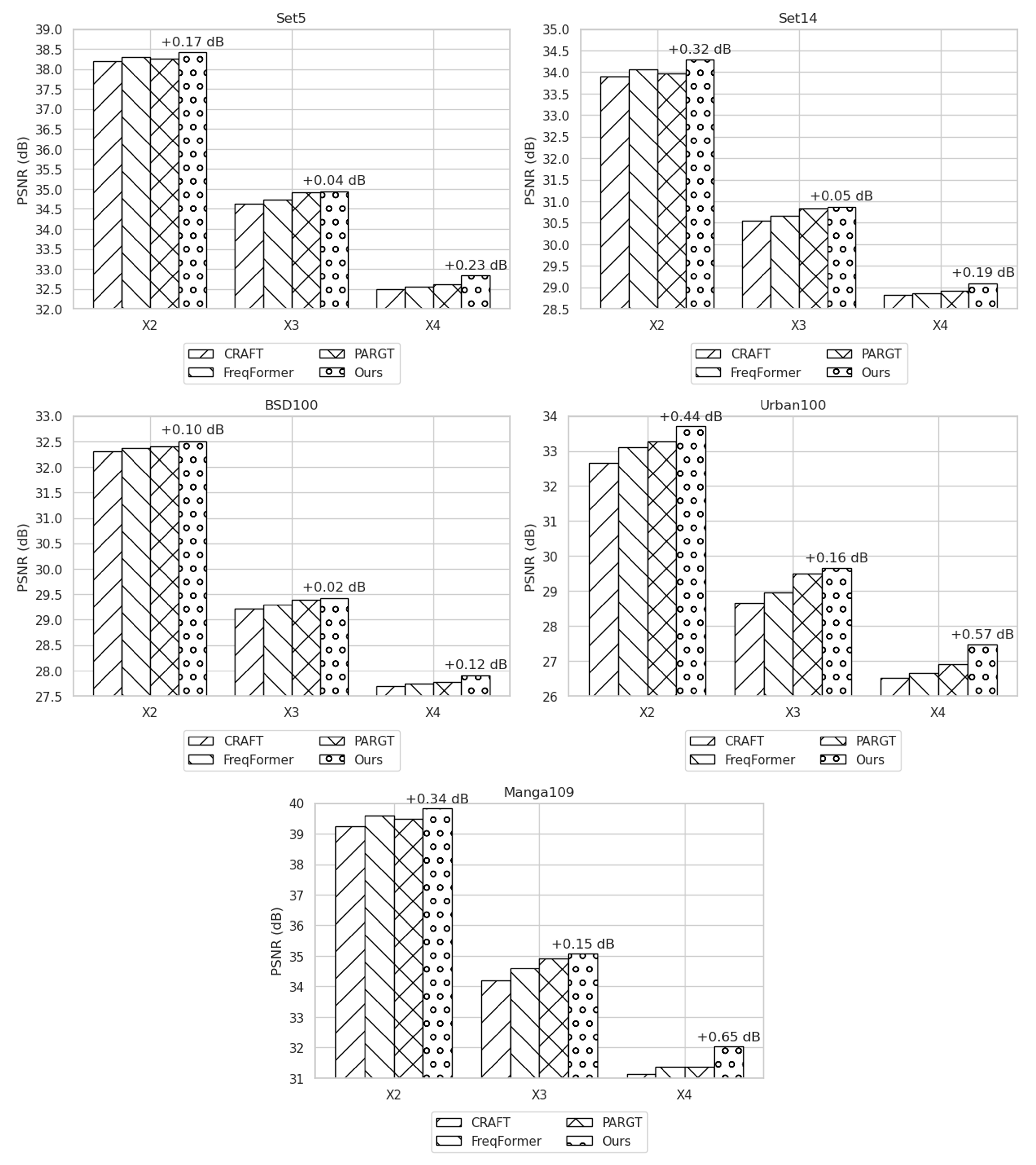
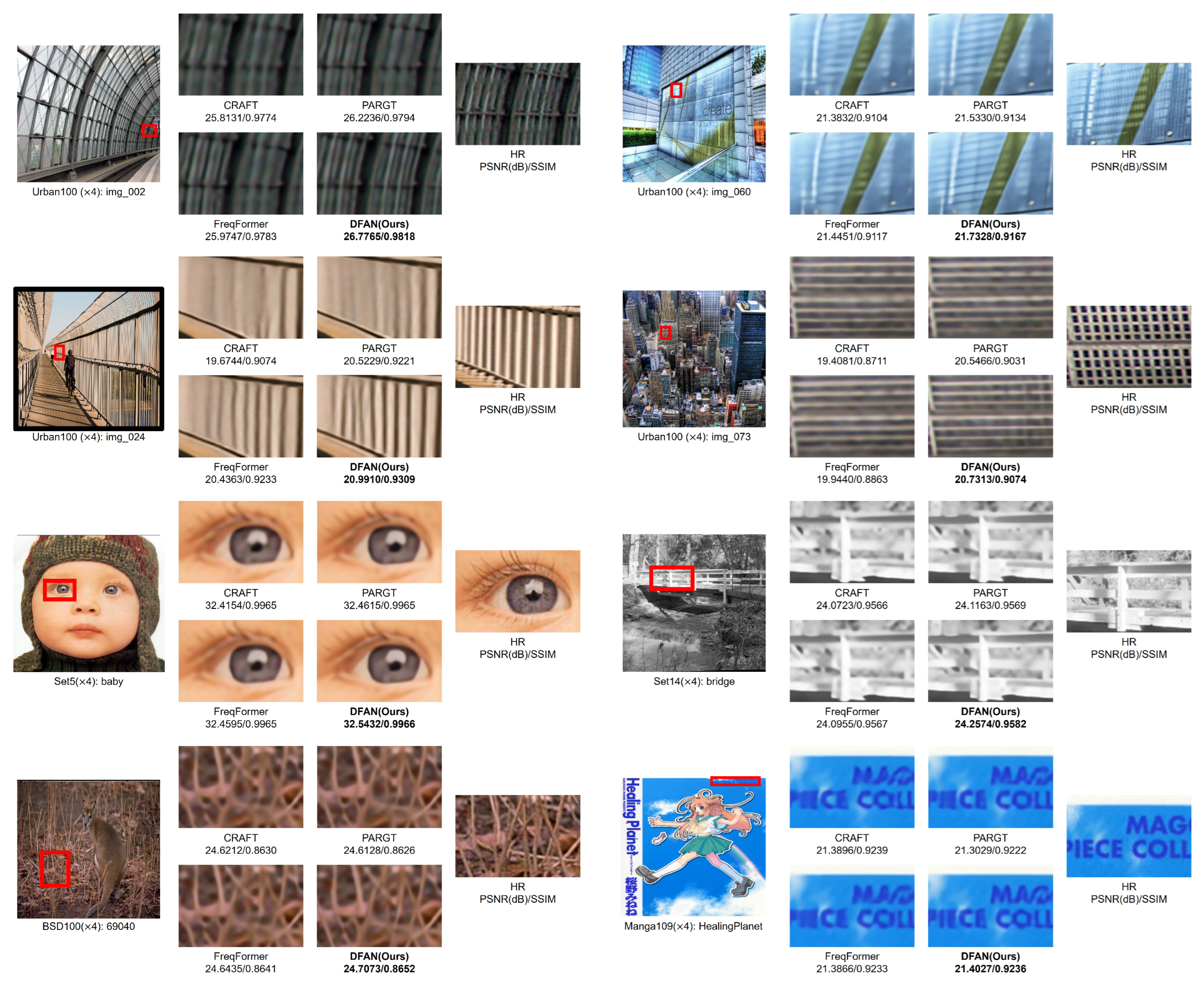
4. Experimental Results

In this section, we empirically validate the proposed DFAN against representative state-of-the-art approaches. We outline the experimental design, specify the training and inference datasets, list the competing methods, and describe the evaluation metrics. Comprehensive quantitative and qualitative results are then presented to demonstrate the efficacy of our model.

4.1. Experimental Settings

Training is conducted on the DF2K dataset, which merges DIV2K, comprising 800 high-quality images, and Flickr2K, comprising 2650 additional high-resolution photographs, yielding a total of 3450 HR images [83,84]. Both source datasets were collected at approximately 2 K resolution ($2048\times 1080$) and encompass a diverse range of scenes, including landscapes, portraits, and architecture. Low-resolution counterparts are generated from these HR images using MATLAB(R2017a)’s bicubic downsampling at scales $\times 2$, $\times 3$, and $\times 4$, producing 3450 aligned LR–HR pairs for training. For evaluation, we use five standard benchmarks. Set5 [85] contains five iconic test images, and Set14 [86] provides 14 additional natural-scene photographs and human portraits. BSD100 [87] offers 100 images spanning diverse outdoor and indoor environments, whereas Urban100 [88] likewise comprises 100 pictures characterized by complex urban architecture with abundant high-frequency details. Finally, Manga109 [89] shall consist of 109 high-contrast manga pages, each featuring intricate line art. A summary is given in

Table 2. Summary of the datasets used in the experimental evaluation. Dataset lists the name of each benchmark or training collection, Images gives the number of high-resolution images it contains, Image Size reports the representative (average or canonical) spatial resolution of those images, Description briefly characterizes the visual content, and Usage specifies whether the dataset is employed for network training or for test-set evaluation.

Dataset	Images	Image Size	Description	Usage
DIV2K [83]	800	2K ($2048\times 1080$)	high quality natural images	Train
Flickr2K [84]	2650	2K ($2048\times 1080$)	high-resolution from Flickr	Train
Set5 [85]	5	$256\times 256$	five iconic images	Test
Set14 [86]	14	$300\times 500$	natural images of mixed	Test
BSD100 [87]	100	$481\times 321$	varied indoor and outdoor	Test
Urban100 [88]	100	$1024\times 1024$	urban-scene in building	Test
Manga109 [89]	109	$1200\times 880$	high-resolution manga pages	Test

. Although the exact resolution varies within each benchmark, the average sizes are approximately $256\times 256$ pixels for Set5, $300\times 500$ pixels for Set14, $481\times 321$ pixels for BSD100, $1024\times 1024$ pixels for Urban100, and $1200\times 880$ pixels for Manga109.

To balance performance and efficiency, DFAN is configured as follows. A single DFAN Group contains six LF Blocks, one HF Block, and one FFM, stacking six such groups yields a total depth of 36 LF Blocks, six HF Blocks, and six FFMs. All convolutional and attention layers share an embedding dimension of 180 channels. The choice of six DFAN Groups, six LF Blocks per group, and an embedding dimension of 180 channels follows the common design of contemporary two-stage SISR networks, which separate shallow and deep feature extraction while keeping the overall model size tractable [10,11]. By contrast, the HF branch is deliberately kept lightweight; only one directional RDB is used because a deeper high-frequency stack tends to amplify aliasing and increases training loss without a proportional performance gain [76]. Inside each LF Block, the Window Multi-Head Self-Attention uses $h=6$ heads and a window size of $16\times 16$. During training, $64\times 64$ patches are randomly cropped from DF2K LR images and augmented by random rotation and horizontal flipping. At inference time, larger images are tiled into the same $64\times 64$ patches, so the per-patch computational cost of the W-MSA remains fixed, independent of the original image resolution.

Table 3. Summary of the DFAN network architecture and training hyperparameters. Component lists each network module or optimization parameter, Setting gives the chosen value, and Notes provides brief explanatory remarks.

Component	Setting	Notes
DFAN Groups	6	-
LF Blocks per Group	6	Total 36
HF Blocks per Group	1	Total 6
FFM per Group	1	Total 6
Embedding dimension	180	Channels
Self-attention heads	6	-
Window size	$16\times 16$	-
Input size	$64\times 64$	Random Rotation and Flip
Batch size	4	-
Iterations	500 K	learning-rate decay schedule below
Initial learning rate	$2\times {10}^{-4}$	halved at [250 K, 400 K, 450 K, 475 K]
Optimizer	Adam	${\beta }_1=0.9$, ${\beta }_2=0.99$

lists the network hyperparameters and the corresponding training settings. Training is conducted for 500 K iterations with a batch size of 4. The initial learning rate is $2\times {10}^{-4}$ and is halved at 250 K, 400 K, 450 K, and 475 K iterations. Optimization is performed with Adam, using ${\beta }_1=0.9$ and ${\beta }_2=0.99$

All experiments are conducted on a workstation equipped with an Intel® i9-14900K CPU, 128 GB of RAM, and an NVIDIA RTX 4090 GPU. Under this configuration, end-to-end training completes in roughly one day, and the process can be further accelerated in a distributed environment. A detailed description of hardware implementation feasibility and model complexity is provided in Appendix A. Quantitative evaluation employs three representative metrics: PSNR, SSIM, and LPIPS. First, the mean-squared error (MSE) between the restored image $I_1$ and its reference $I_2$ is computed as

$$\mathrm{MSE}={\displaystyle \frac{1}{M\times N}}\sum _{m=1}^M\sum _{n=1}^N{\left[I_1(m,n)-I_2(m,n)\right]}^2,$$

(22)

where M and N denote the image height and width, respectively. Using this error, the peak signal-to-noise ratio (PSNR) is then defined by

$$\mathrm{PSNR}=10{log}_{10}\left(\frac{R^2}{\mathrm{MSE}}\right),$$

(23)

with R representing the maximum possible pixel value. SSIM combines luminance, contrast, and structural terms to assess structural similarity, as shown in Equation (24).

$$\mathrm{SSIM}(x,y)={\displaystyle \frac{\left(2{\mu }_x{\mu }_y+C_1\right)\left(2{\sigma }_{xy}+C_2\right)}{\left({\mu }_x^2+{\mu }_y^2+C_1\right)\left({\sigma }_x^2+{\sigma }_y^2+C_2\right)}}$$

(24)

In Equation (24), ${\mu }_x$ and ${\mu }_y$ denote the local means of images x and y, measuring luminance similarity. ${\sigma }_x^2$ and ${\sigma }_y^2$ represent their variances, quantifying contrast similarity, whereas ${\sigma }_{xy}$ is the covariance between x and y, capturing structural similarity. The constants $C_1$ and $C_2$ are small positive terms introduced to stabilize the computation when the denominator approaches zero. LPIPS computes a perceptual distance in the feature space of a pre-trained network, yielding a score that correlates more closely with human visual quality, as expressed in Equation (25).

$$\mathrm{LPIPS}(x,y)=\sum _l{\displaystyle \frac{1}{H_l{W}_l}}\sum _{h=1}^{H_l}\sum _{w=1}^{W_l}{∥w_l\odot \left({\widehat{y}}_l{\left(x\right)}_{h,w}-{\widehat{y}}_l{\left(y\right)}_{h,w}\right)∥}_2^2$$

(25)

where x and y are the two image patches being compared; ${\widehat{y}}_l{(·)}_{h,w}$ is the vector at location $(h,w)$ in the normalized feature map extracted from the l-th layer of a pre-trained network for the input image, $H_l$ and $W_l$ denote the height and width of that l-th layer feature map, $w_l$ is a channel-wise weight vector that adjusts the importance of each feature channel through learned values, ⊙ indicates channel-wise multiplication, and $\left|\right|·{\left|\right|}_2^2$ is the squared L2-norm, measuring the difference between two feature vectors.

4.2. Comparison Results and Analysis

Table 4. Quantitative comparison with state-of-the-art methods on benchmark datasets. This table represents the PSNR performance indicator, and the higher the value, the better the performance. Bold highlights the proposed method (Ours), and underlining denotes the highest performance in each column.

Method	Scale	Set5	Set14	BSD100	Urban100	Manga109
CRAFT (2023)	$\times 2$	38.2070	33.9034	32.2995	32.6665	39.2395
FreqFormer (2024)	$\times 2$	38.2925	34.0676	32.3750	33.1099	39.5769
PARGT (2025)	$\times 2$	38.2500	33.9664	32.3943	33.2595	39.4927
Ours	$\times 2$	38.4202	34.2870	32.4971	33.7021	39.8351
CRAFT (2023)	$\times 3$	34.6276	30.5380	29.2228	28.6541	34.2061
FreqFormer (2024)	$\times 3$	34.7365	30.6560	29.3017	28.9503	34.5858
PARGT (2025)	$\times 3$	34.9097	30.8217	29.3973	29.5021	34.9208
Ours	$\times 3$	34.9471	30.8670	29.4218	29.6650	35.0757
CRAFT (2023)	$\times 4$	32.4914	28.8153	27.6962	26.5213	31.1378
FreqFormer (2024)	$\times 4$	32.5532	28.8654	27.7469	26.6441	31.3610
PARGT (2025)	$\times 4$	32.6064	28.9114	27.7797	26.9051	31.3785
Ours	$\times 4$	32.8318	29.0985	27.8968	27.4800	32.0279

,

Table 5. Quantitative comparison with state-of-the-art methods on benchmark datasets. This table represents the SSIM performance indicator, and the higher the value, the better the performance. Bold highlights the proposed method (Ours), and underlining denotes the highest performance in each column.

Method	Scale	Set5	Set14	BSD100	Urban100	Manga109
CRAFT (2023)	$\times 2$	0.9613	0.9207	0.9012	0.9330	0.9783
FreqFormer (2024)	$\times 2$	0.9615	0.9218	0.9022	0.9366	0.9791
PARGT (2025)	$\times 2$	0.9615	0.9207	0.9023	0.9384	0.9789
Ours	$\times 2$	0.9621	0.9232	0.9036	0.9414	0.9797
CRAFT (2023)	$\times 3$	0.9290	0.8455	0.8086	0.8617	0.9484
FreqFormer (2024)	$\times 3$	0.9299	0.8474	0.8103	0.8678	0.9502
PARGT (2025)	$\times 3$	0.9311	0.8505	0.8128	0.8774	0.9522
Ours	$\times 3$	0.9317	0.8519	0.8133	0.8803	0.9529
CRAFT (2023)	$\times 4$	0.8987	0.7866	0.7411	0.7984	0.9163
FreqFormer (2024)	$\times 4$	0.8990	0.7880	0.7428	0.8041	0.9178
PARGT (2025)	$\times 4$	0.9002	0.7892	0.7444	0.8110	0.9188
Ours	$\times 4$	0.9025	0.7934	0.7472	0.8242	0.9246

and

Table 6. Quantitative comparison with state-of-the-art methods on benchmark datasets. This table represents the LPIPS performance indicator, and the lower the value, the better the performance. Bold highlights the proposed method (Ours), and underlining denotes the highest performance in each column.

Method	Scale	Set5	Set14	BSD100	Urban100	Manga109
CRAFT (2023)	$\times 2$	0.1691	0.2834	0.3630	0.2218	0.1412
FreqFormer (2024)	$\times 2$	0.0562	0.1369	0.1403	0.0564	0.0227
PARGT (2025)	$\times 2$	0.0539	0.1356	0.1383	0.0544	0.0223
Ours	$\times 2$	0.0530	0.0866	0.1354	0.0504	0.0214
CRAFT (2023)	$\times 3$	0.1255	0.2476	0.2765	0.1522	0.0824
FreqFormer (2024)	$\times 3$	0.1261	0.2528	0.2766	0.1494	0.0821
PARGT (2025)	$\times 3$	0.1223	0.2460	0.2705	0.1371	0.0794
Ours	$\times 3$	0.1211	0.2052	0.2697	0.1340	0.0798
CRAFT (2023)	$\times 4$	0.1702	0.3212	0.3643	0.2234	0.1416
FreqFormer (2024)	$\times 4$	0.1697	0.3206	0.3649	0.2223	0.1408
PARGT (2025)	$\times 4$	0.1662	0.3139	0.3572	0.2123	0.1389
Ours	$\times 4$	0.1651	0.3104	0.3566	0.1990	0.1364

present the experimental results on the five benchmark datasets, comparing the proposed DFAN with three frequency-domain super-resolution models: CRAFT [36], FreqFormer [37], and PARGT [38]. Table 4 lists the PSNR scores, Table 5 provides the SSIM scores, and Table 6 summarizes the LPIPS values. All evaluations are carried out at scaling factors $\times 2$, $\times 3$, and $\times 4$.

For every scaling factor, DFAN now achieves the best PSNR and SSIM on all five benchmarks, decisively surpassing CRAFT, FreqFormer, and PARGT across Set5, Set14, BSD100, Urban100, and Manga109. In the perceptual LPIPS metric, DFAN likewise records the lowest (best) scores at $\times 2$ and $\times 4$ on every dataset, and at $\times 3$ on four of the five sets; the sole exception is the $\times 3$ experiment on Manga109, where DFAN trails PARGT by a narrow margin +0.002. This isolated shortfall aside, the results confirm that the proposed frequency-aware architecture delivers state-of-the-art fidelity and perceptual quality over all scales and image types. These findings confirm that the proposed frequency-aware architecture maintains both distortion fidelity and perceptual quality over a wide range of scales and image types. Moreover, the pattern of gains is consistent with the specific strengths of each DFAN component. Datasets rich in repetitive architectural detail, such as Urban100, benefit most from the high-frequency branch with directional convolutions, which sharpens lattice-like edges that challenge transformer-only baselines. Conversely, the smoother tonal transitions in Set14 and BSD100 highlight the Swin-based low-frequency branch, whose large receptive field maintains structural coherence without over-smoothing. The Manga109 comics benchmark, characterised by high-contrast line art and text, showcases the synergy of the Feature Fusion Module, which balances bold strokes (HF) with uniform fill regions (LF) to preserve both crisp outlines and flat inking. Together, these observations indicate that each module, HF Block, LF Block, and FFM, contributes in a complementary fashion, enabling DFAN to adapt its restoration strategy to the dominant frequency characteristics of each dataset.

Figure 4 plots the PSNR obtained by each network on the five test sets at the three enlargement factors. Across almost every dataset–scale combination, DFAN delivers a positive gain over the runner-up method. The most pronounced improvement is observed on Manga109 at $\times 4$, where DFAN outperforms the second-best model by 0.64 dB, a sizable margin that underscores the effectiveness of the directional HF branch in recovering the razor-thin strokes and screen tone patterns characteristic of manga artwork.

Figure 5 provides a qualitative comparison of ×4 super-resolution outputs. In Urban100 images “img_002,” “img_024,” “img_060,” and “img_073,” the proposed DFAN reconstructs the dense lattice patterns on glass façades, railings, and window grids with markedly greater clarity than CRAFT, FreqFormer, and PARGT. Competing methods exhibit blurred lines, aliasing, or zipper artifacts along vertical and diagonal structures, whereas DFAN preserves straight edges, restores the correct line spacing, and suppresses color fringing. These visual gains corroborate the quantitative scores: The high-frequency branch with directional convolution sharpens fine textures, and the adaptive fusion module prevents the low-pass smoothing often observed in Transformer-only models. In the Set5 “baby” image, DFAN retains the fine eyebrow hairs that other models blur. The Set14 “bridge” scene demonstrates DFAN delivering crisp, ribbed-girder edges without ringing, whereas baseline methods exhibit aliasing. For BSD100 sample “69040”, which is dominated by thin, randomly oriented reeds, DFAN maintains the delicate filament structure that competing models oversmooth or checkerboard. Finally, in the Manga109 panel from “HealingPlanet”, DFAN reproduces the slender stroke edges of handwritten kana and the sharp screentone boundaries, whereas other outputs smear or distort these comic-style high-frequency details. Collectively, these diverse examples confirm DFAN’s consistent ability to preserve texture fidelity, edge sharpness, and small text across natural, structural, and illustrated imagery, underscoring its superiority in recovering high-frequency detail while maintaining geometric fidelity.

Table 7. Ablation study on the proposed HF Block and FFM. Baseline refers to a DFAN configuration with the default settings described in Section 4.1. Bold and underlining indicate the highest performance, denotes the component is applied, and X denotes it is not applied

	Baseline
Frequency Loss	✓	✓	✓	X	✓
HF Block	X	✓	X	✓	✓
FFM	X	X	✓	✓	✓
PSNR	33.9047	33.7059	34.1688	34.1484	34.2870

presents an ablation study that quantifies the individual and combined contributions of the HF Block and the FFM. To keep training time manageable, we survey the $\times 2$ enlargement of the Set14 dataset and report performance with the PSNR metric. Beginning with the baseline configuration, which excludes both components, we observe a PSNR of 33.9047 dB. Introducing only the HF Block lowers performance to 33.7059 dB, suggesting that injecting frequency-specific features without a dedicated reconciliation mechanism can disturb cross-band balance and introduce artefacts. Enabling only the FFM, in contrast, raises the PSNR to 34.1688 dB, demonstrating that an adaptive depthwise–pointwise fusion of spatial and spectral cues is beneficial even in the absence of explicit HF enhancement. When both the HF Block and the FFM are activated, the PSNR peaks at 34.2870 dB. This improvement reveals an apparent synergy; the directional convolutions and residual-dense filtering in the HF Block first sharpen horizontal, vertical, and diagonal details. At the same time, the subsequent FFM aligns these refined HF maps with the LF branch on a channel-wise basis and re-weights them spatially. The depthwise stage corrects residual ghosting within each channel, and the pointwise stage learns cross-channel dependencies that restore the proper energy ratio between low- and high-frequency bands. In other words, the FFM unlocks the benefit of the HF Block by preventing the over-emphasis of isolated textures and integrating them coherently into the global representation. Together, the two modules deliver the most significant overall gain because they form a complementary pair, one specializing in frequency-selective enhancement, the other in adaptive cross-band fusion. To isolate the effect of the proposed frequency-aware loss, we also trained the full configuration (HF Block + FFM) without this loss term, obtaining 34.1484 dB. Re-enabling the loss raises performance to 34.2870 dB, confirming that explicitly constraining sub-band reconstruction stabilises optimization and guides the network toward sharper, artefact-free details.

Table 8. Ablation study on PSNR(dB) of different window sizes at $\times 2$ scale. Bold and underlining text indicates the highest performance.

Size	Set5	Set14	BSD100	Urban100	Manga109
$(8,8)$	38.3089	34.1270	32.4394	33.2871	39.6650
$(16,16)$	38.4202	34.2870	32.4971	33.7021	39.8351

reports an ablation study on the window size used in the Window-MSA layer of the LF branch. Two settings are compared: a smaller $8\times 8$ window and a larger $16\times 16$ window. The larger window consistently delivers higher PSNR on every benchmark, confirming that a broader local context helps the LF branch capture long-range correlations without resorting to full-image self-attention. Gains are especially pronounced on Urban100 and Manga109, rising by approximately 0.4 dB and 0.17 dB, respectively. These datasets contain large buildings with repetitive grids and densely drawn manga strokes, scenarios where a wider receptive field improves the aggregation of low-frequency structure and reduces residual aliasing. The uniform performance improvements outweigh the marginal increase in computational cost, so $16\times 16$ is adopted as the default window size in DFAN.

Table 9. Ablation study on PSNR(dB) for different frequency-loss weights at $\times 2$ scale. Bold and underlining text indicates the highest performance.

Weight	Set5	Set14	BSD100	Urban100	Manga109
$0.05$	38.3649	34.1117	32.4640	33.3974	39.7731
$0.10$	38.3748	34.2116	32.4623	33.4187	39.8063
$0.50$	38.3984	34.1451	32.4790	33.4569	39.8424
$1.0$	38.4202	34.2870	32.4971	33.7021	39.8351

reports a sweep over the global weight assigned to the frequency-aware loss. A very small weight $0.05$ already nudges the network toward sharper details but yields only modest gains, especially on the texture-rich Urban100 and Manga109 sets. Increasing the weight to $0.10$, the value used in our main experiments, consistently improves Set14, Urban100, and Manga109, indicating that the network benefits from a stronger high-frequency constraint. Pushing the coefficient further to $0.50$ slightly boosts Set5, BSD100, and Urban100, yet the improvements remain uneven. When the weight reaches $1.0$, every benchmark records its highest PSNR: +0.056 dB on Set5, +0.176 dB on Set14, +0.035 dB on BSD100, +0.304 dB on Urban100, and +0.028 dB on Manga109 relative to the $0.10$ setting. These results suggest that the full-scale penalty best balances low- and high-frequency fidelity across diverse image statistics. Consequently, we adopt the $1.0$ weighting in the final DFAN configuration.

Table 10. Ablation study on PSNR(dB) for different kernel size at $\times 2$ scale in HFBlock.

Kernel Size	Set5	Set14	BSD100	Urban100	Manga109
$(3\times 3)$	38.2807	34.0165	32.4096	33.0728	39.5516
learnable kernel	38.1856	33.8996	32.3276	32.5924	39.3014
Ours	38.2955	34.1280	32.4230	33.1009	39.5852

reports PSNR(dB) at $\times 2$ magnification for three kernel configurations after 250 K training iterations, half of the full 500 K schedule, to track early-stage performance trends. Across all five benchmarks, the proposed directional design achieves the highest PSNR, outperforming the $(3\times 3)$ variant by 0.01–0.06 dB and the learnable version by 0.18–0.54 dB. The learnable kernels train more quickly and could potentially improve with longer schedules; yet, their PSNR already falls below even the simple $(3\times 3)$ baseline at this halfway point, indicating that unconstrained adaptation may overfit noise directions rather than the dominant edge orientations. By contrast, the fixed, orientation-aware filters consistently extract horizontal, vertical, and diagonal details that generalize better to the validation images, confirming the efficacy of the proposed high-frequency design.

Table 11. PSNR(dB) comparison on the five standard benchmarks at $\times 2$, $\times 3$, and $\times 4$ magnification between the proposed DFAN and two recent Transformer-based SISR methods, SwinIR (2021) and HAT (2023). Higher values indicate better performance. Bold and highlighted text indicates the highest performance.

Method	Scale	Set5	Set14	BSD100	Urban100	Manga109
SwinIR (2021)	$\times 2$	38.3439	34.2175	32.4669	33.5044	39.6978
HAT (2023)	$\times 2$	38.4153	34.3592	32.4911	33.7949	39.8079
Ours	$\times 2$	38.4202	34.2870	32.4971	33.7021	39.8351
SwinIR (2021)	$\times 3$	34.8726	30.7984	29.3661	29.3223	34.8562
HAT (2023)	$\times 3$	34.9408	30.8853	29.4215	29.6555	35.0874
Ours	$\times 3$	34.9471	30.8670	29.4218	29.6650	35.0757
SwinIR (2021)	$\times 4$	32.6939	29.0052	27.8341	27.0502	31.7022
HAT (2023)	$\times 4$	32.7838	29.0747	27.8862	27.4110	31.9933
Ours	$\times 4$	32.8318	29.0985	27.8968	27.4800	32.0279

compares DFAN with two state-of-the-art Transformer baselines, SwinIR (2021) and HAT (2023), at magnification factors $\times 2$, $\times 3$, and $\times 4$. DFAN surpasses SwinIR on every dataset at every scale, confirming that explicitly modeling dual-frequency pathways offers a consistent advantage over a single-branch Transformer. Relative to HAT, the picture is mixed at the lower scales but favorable overall. At $\times 2$, DFAN yields higher PSNR on Set5, BSD100, and Manga109, while HAT maintains marginal leads on Set14 (+0.072 dB) and Urban100 (+0.093 dB). At $\times 3$, DFAN again wins on Set5, BSD100, and Urban100, trails slightly on Set14 (−0.018 dB), and is nearly tied on Manga109 (−0.012 dB). Under the more demanding $\times 4$ setting, DFAN overtakes HAT on all five benchmarks, with its most significant margin on Urban100 (+0.069 dB). These results suggest a complementary relationship between the two design philosophies. The HAT model’s wide-window attention is beneficial for heavily slanted or highly repetitive urban scenes at moderate scales. In contrast, the DFAN model’s frequency-aware processing becomes increasingly effective as scale grows and as images contain either fine textures or large high-frequency regions. Taken together, the findings underline that frequency separation and adaptive fusion can match or surpass the performance of larger-window Transformers while incurring less token-interaction overhead, and they motivate future work on hybrid models that integrate the strengths of both approaches.

5. Conclusions

This study proposes the Dual-Frequency Adaptive Network, which explicitly leverages band-specific frequency characteristics to mitigate high-frequency loss significantly. A Stationary Wavelet Transform first decomposes the input image into one low-frequency band and three directional high-frequency bands. The low-frequency branch is processed with a Swin Transformer layer, while the high-frequency branch employs directional convolutions and Residual Dense Blocks. The two branches are then adaptively merged by a Feature Fusion Module. Additionally, a frequency-aware multi-term loss is combined with the conventional pixel reconstruction loss, enabling the network to learn high-frequency content explicitly. Experiments conducted on the standard benchmarks Set5, Set14, BSD100, Urban100, and Manga109 show that DFAN consistently outperforms recent methods in terms of PSNR, SSIM, and LPIPS, thereby demonstrating its effectiveness. These gains stem from the synergy of three key contributions: an SWT-based dual pipeline, a directional high-frequency module with frequency–spatial fusion, and a frequency-aware multi-loss objective.

The frequency-separated, parallel architecture of DFAN offers clear practical advantages, enabling a balanced restoration of low-frequency structures and high-frequency textures. Directional convolutions selectively amplify edge orientations to recover fine details, and the frequency-aware loss ensures more stable high-frequency learning than existing Transformer-based models. Nonetheless, the use of fixed SWT kernels and predetermined branch depths limits the framework’s ability to adapt optimally when object scales or degradation types vary widely, and the present evaluation, restricted to standard bicubic down-sampling, does not yet verify DFAN robustness under real-world degradations such as blur, sensor noise, or aggressive JPEG compression. Future work will enhance DFAN by introducing learnable wavelet decompositions, including lightweight multi-level SWT variants, and incorporating explicit domain-adaptation schemes for blur, noise, and compression artifacts. We also plan to explore hybrid techniques that fuse DFAN with complementary spatial–frequency modules or multi-loss objectives, and to investigate high-frequency-oriented learnable kernels, such as dilated or deformable convolutions, to further improve directional detail recovery without incurring prohibitive computational costs. Additionally, we will examine adaptive, sub-band-specific loss weights, allowing each frequency component to be optimized according to its relative perceptual importance.

References

1. Neshatavar, R.; Yavartanoo, M.; Son, S.; Lee, K.M. Icf-srsr: Invertible scale-conditional function for self-supervised real-world single image super-resolution. In Proceedings of the IEEE/CVF Winter Conference on Applications of Computer Vision, Waikoloa, HI, USA, 3–7 January 2024; pp. 1557–1567. [Google Scholar]
2. Yao, J.E.; Tsao, L.Y.; Lo, Y.C.; Tseng, R.; Chang, C.C.; Lee, C.Y. Local implicit normalizing flow for arbitrary-scale image super-resolution. In Proceedings of the IEEE/CVF Conference on Computer Vision and Pattern Recognition, Vancouver, BC, Canada, 18–22 June 2023; pp. 1776–1785. [Google Scholar]
3. Al-Mekhlafi, H.; Liu, S. Single image super-resolution: A comprehensive review and recent insight. Front. Comput. Sci. 2024, 18, 181702. [Google Scholar] [CrossRef]
4. Zhang, W.; Li, X.; Shi, G.; Chen, X.; Qiao, Y.; Zhang, X.; Wu, X.M.; Dong, C. Real-world image super-resolution as multi-task learning. Adv. Neural Inf. Process. Syst. 2023, 36, 21003–21022. [Google Scholar]
5. Kim, J.; Lee, J.K.; Lee, K.M. Accurate image super-resolution using very deep convolutional networks. In Proceedings of the IEEE Conference on Computer Vision and Pattern Recognition, Las Vegas, NV, USA, 26 June–1 July 2016; pp. 1646–1654. [Google Scholar]
6. Lim, B.; Son, S.; Kim, H.; Nah, S.; Mu Lee, K. Enhanced deep residual networks for single image super-resolution. In Proceedings of the IEEE Conference on Computer Vision and Pattern Recognition Workshops, Honolulu, HI, USA, 21–26 July 2017; pp. 136–144. [Google Scholar]
7. Dong, C.; Loy, C.C.; He, K.; Tang, X. Image super-resolution using deep convolutional networks. IEEE Trans. Pattern Anal. Mach. Intell. 2015, 38, 295–307. [Google Scholar] [CrossRef] [PubMed]
8. Zhang, Y.; Tian, Y.; Kong, Y.; Zhong, B.; Fu, Y. Residual dense network for image super-resolution. In Proceedings of the IEEE Conference on Computer Vision and Pattern Recognition, Salt Lake City, UT, USA, 18–22 June 2018; pp. 2472–2481. [Google Scholar]
9. Zhang, Y.; Li, K.; Li, K.; Wang, L.; Zhong, B.; Fu, Y. Image super-resolution using very deep residual channel attention networks. In Proceedings of the European Conference on Computer Vision (ECCV), Munich, Germany, 8–14 September 2018; pp. 286–301. [Google Scholar]
10. Liang, J.; Cao, J.; Sun, G.; Zhang, K.; Van Gool, L.; Timofte, R. Swinir: Image restoration using swin transformer. In Proceedings of the IEEE/CVF International Conference on Computer Vision, Montréal, BC, Canada, 11–17 October 2021; pp. 1833–1844. [Google Scholar]
11. Chen, X.; Wang, X.; Zhou, J.; Qiao, Y.; Dong, C. Activating more pixels in image super-resolution transformer. In Proceedings of the IEEE/CVF Conference on Computer Vision and Pattern Recognition, Vancouver, BC, Canada, 18–22 June 2023; pp. 22367–22377. [Google Scholar]
12. Huynh-Thu, Q.; Ghanbari, M. Scope of validity of PSNR in image/video quality assessment. Electron. Lett. 2008, 44, 800–801. [Google Scholar] [CrossRef]
13. Wang, Z.; Bovik, A.C.; Sheikh, H.R.; Simoncelli, E.P. Image quality assessment: From error visibility to structural similarity. IEEE Trans. Image Process. 2004, 13, 600–612. [Google Scholar] [CrossRef] [PubMed]
14. Ledig, C.; Theis, L.; Huszár, F.; Caballero, J.; Cunningham, A.; Acosta, A.; Aitken, A.; Tejani, A.; Totz, J.; Wang, Z.; et al. Photo-realistic single image super-resolution using a generative adversarial network. In Proceedings of the IEEE Conference on Computer Vision and Pattern Recognition, Honolulu, HI, USA, 21–26 July 2017; pp. 4681–4690. [Google Scholar]
15. Isola, P.; Zhu, J.Y.; Zhou, T.; Efros, A.A. Image-to-image translation with conditional adversarial networks. In Proceedings of the IEEE Conference on Computer Vision and Pattern Recognition, Honolulu, HI, USA, 21–26 July 2017; pp. 1125–1134. [Google Scholar]
16. Jiang, L.; Dai, B.; Wu, W.; Loy, C.C. Focal frequency loss for image reconstruction and synthesis. In Proceedings of the IEEE/CVF International Conference on Computer Vision, Montréal, ON, Canada, 11–17 October 2021; pp. 13919–13929. [Google Scholar]
17. Haris, M.; Shakhnarovich, G.; Ukita, N. Deep back-projection networks for super-resolution. In Proceedings of the IEEE Conference on Computer Vision and Pattern Recognition, Salt Lake City, UT, USA, 18–22 June 2018; pp. 1664–1673. [Google Scholar]
18. Jiang, J.; Yu, Y.; Wang, Z.; Tang, S.; Hu, R.; Ma, J. Ensemble super-resolution with a reference dataset. IEEE Trans. Cybern. 2019, 50, 4694–4708. [Google Scholar] [CrossRef]
19. Wang, W.; Zhang, H.; Yuan, Z.; Wang, C. Unsupervised real-world super-resolution: A domain adaptation perspective. In Proceedings of the IEEE/CVF International Conference on Computer Vision, Montréal, BC, Canada, 11–17 October 2021; pp. 4318–4327. [Google Scholar]
20. Kimura, M. Understanding test-time augmentation. In Proceedings of the International Conference on Neural Information Processing, Bali, Indonesia, 8–12 December 2021; Springer: Berlin/Heidelberg, Germany, 2021; pp. 558–569. [Google Scholar]
21. Kong, L.; Dong, J.; Ge, J.; Li, M.; Pan, J. Efficient frequency domain-based transformers for high-quality image deblurring. In Proceedings of the IEEE/CVF Conference on Computer Vision and Pattern Recognition, Vancouver, BC, Canada, 18—22 June 2023; pp. 5886–5895. [Google Scholar]
22. Xiang, S.; Liang, Q. Remote sensing image compression based on high-frequency and low-frequency components. IEEE Trans. Geosci. Remote Sens. 2024, 62, 1–15. [Google Scholar] [CrossRef]
23. Dumitrescu, D.; Boiangiu, C.A. A study of image upsampling and downsampling filters. Computers 2019, 8, 30. [Google Scholar] [CrossRef]
24. Zhang, R.; Isola, P.; Efros, A.A.; Shechtman, E.; Wang, O. The unreasonable effectiveness of deep features as a perceptual metric. In Proceedings of the IEEE Conference on Computer Vision and Pattern Recognition, Salt Lake City, UT, USA, 18–22 June 2018; pp. 586–595. [Google Scholar]
25. Li, Z.; Zhao, X.; Zhao, C.; Tang, M.; Wang, J. Transfering low-frequency features for domain adaptation. In Proceedings of the 2022 IEEE International Conference on Multimedia and Expo (ICME), Taipei, Taiwan, 18–22 July 2022; pp. 1–6. [Google Scholar]
26. Oh, Y.; Park, G.Y.; Cho, N.I. Restoration of high-frequency components in under display camera images. In Proceedings of the 2022 Asia-Pacific Signal and Information Processing Association Annual Summit and Conference (APSIPA ASC), Chiang Mai, Thailand, 7–10 November 2022; pp. 1040–1046. [Google Scholar]
27. Xie, Z.; Wang, S.; Yu, Q.; Tan, X.; Xie, Y. CSFwinformer: Cross-space-frequency window transformer for mirror detection. IEEE Trans. Image Process. 2024, 33, 1853–1867. [Google Scholar] [CrossRef]
28. Deng, X.; Yang, R.; Xu, M.; Dragotti, P.L. Wavelet domain style transfer for an effective perception-distortion tradeoff in single image super-resolution. In Proceedings of the IEEE/CVF International Conference on Computer Vision, Seoul, Republic of Korea, 27 October–2 November 2019; pp. 3076–3085. [Google Scholar]
29. Wang, X. Interpolation and sharpening for image upsampling. In Proceedings of the 2022 2nd International Conference on Computer Graphics, Image and Virtualization (ICCGIV), Chongqing, China, 23–25 September 2022; pp. 73–77. [Google Scholar]
30. Jahnavi, M.; Rao, D.R.; Sujatha, A. A comparative study of super-resolution interpolation techniques: Insights for selecting the most appropriate method. Procedia Comput. Sci. 2024, 233, 504–517. [Google Scholar] [CrossRef]
31. Panda, J.; Meher, S. A new residual image sharpening scheme for image up-sampling. In Proceedings of the 2022 8th International Conference on Signal Processing and Communication (ICSC), Bangalore, India, 11–15 July 2022; pp. 244–249. [Google Scholar]
32. Panda, J.; Meher, S. Recent advances in 2d image upscaling: A comprehensive review. SN Comput. Sci. 2024, 5, 735. [Google Scholar] [CrossRef]
33. Witwit, W.; Hallawi, H.; Zhao, Y. Enhancement for Astronomical Low-Resolution Images Using Discrete-Stationary Wavelet Transforms and New Edge-Directed Interpolation. Trait. Signal 2025, 42, 11. [Google Scholar] [CrossRef]
34. Liu, Z.S.; Wang, Z.; Jia, Z. Arbitrary point cloud upsampling via dual back-projection network. In Proceedings of the 2023 IEEE International Conference on Image Processing (ICIP), Kuala Lumpur, Malaysia, 8–11 October 2023; pp. 1470–1474. [Google Scholar]
35. Liu, Y.; Pang, Y.; Li, J.; Chen, Y.; Yap, P.T. Architecture-Agnostic Untrained Network Priors for Image Reconstruction with Frequency Regularization. In Proceedings of the European Conference on Computer Vision, Milan, Italy, 29 September–4 October 2024; Springer: Berlin/Heidelberg, Germany, 2024; pp. 341–358. [Google Scholar]
36. Li, A.; Zhang, L.; Liu, Y.; Zhu, C. Feature modulation transformer: Cross-refinement of global representation via high-frequency prior for image super-resolution. In Proceedings of the IEEE/CVF International Conference on Computer Vision, Paris, France, 2–3 October 2023; pp. 12514–12524. [Google Scholar]
37. Dai, T.; Wang, J.; Guo, H.; Li, J.; Wang, J.; Zhu, Z. FreqFormer: Frequency-aware transformer for lightweight image super-resolution. In Proceedings of the International Joint Conference on Artificial Intelligence, Jeju Island, Republic of Korea, 3–9 August 2024; pp. 731–739. [Google Scholar]
38. Wang, J.; Hao, Y.; Bai, H.; Yan, L. Parallel attention recursive generalization transformer for image super-resolution. Sci. Rep. 2025, 15, 8669. [Google Scholar] [CrossRef] [PubMed]
39. Freeman, W.T.; Jones, T.R.; Pasztor, E.C. Example-based super-resolution. IEEE Comput. Graph. Appl. 2002, 22, 56–65. [Google Scholar] [CrossRef]
40. Yang, J.; Wright, J.; Huang, T.S.; Ma, Y. Image super-resolution via sparse representation. IEEE Trans. Image Process. 2010, 19, 2861–2873. [Google Scholar] [CrossRef]
41. Timofte, R.; De Smet, V.; Van Gool, L. Anchored neighborhood regression for fast example-based super-resolution. In Proceedings of the IEEE International Conference on Computer Vision, Sydney, Australia, 1–8 December 2013; pp. 1920–1927. [Google Scholar]
42. Schulter, S.; Leistner, C.; Bischof, H. Fast and accurate image upscaling with super-resolution forests. In Proceedings of the IEEE Conference on Computer Vision and Pattern Recognition, Boston, MA, USA, 8–10 June 2015; pp. 3791–3799. [Google Scholar]
43. Li, H.; Lam, K.M.; Wang, M. Image super-resolution via feature-augmented random forest. Signal Process. Image Commun. 2019, 72, 25–34. [Google Scholar] [CrossRef]
44. Dong, C.; Loy, C.C.; Tang, X. Accelerating the super-resolution convolutional neural network. In Proceedings of the Computer Vision–ECCV 2016: 14th European Conference, Amsterdam, The Netherlands, 11–14 October 2016; Proceedings, Part II 14. pp. 391–407. [Google Scholar]
45. Shi, W.; Caballero, J.; Huszár, F.; Totz, J.; Aitken, A.P.; Bishop, R.; Rueckert, D.; Wang, Z. Real-time single image and video super-resolution using an efficient sub-pixel convolutional neural network. In Proceedings of the IEEE Conference on Computer Vision and Pattern Recognition, Las Vegas, NV, USA, 26 June–1 July 2016; pp. 1874–1883. [Google Scholar]
46. Mao, X.; Shen, C.; Yang, Y.B. Image restoration using very deep convolutional encoder-decoder networks with symmetric skip connections. In Proceedings of the Advances in Neural Information Processing Systems, Barcelona, Spain, 6–8 December 2016. [Google Scholar]
47. Kim, J.; Lee, J.K.; Lee, K.M. Deeply-recursive convolutional network for image super-resolution. In Proceedings of the IEEE Conference on Computer Vision and Pattern Recognition, Las Vegas, NV, USA, 26 June–1 July 2016; pp. 1637–1645. [Google Scholar]
48. Tai, Y.; Yang, J.; Liu, X. Image super-resolution via deep recursive residual network. In Proceedings of the IEEE Conference on Computer Vision and Pattern Recognition, Honolulu, HI, USA, 21–26 July 2017; pp. 3147–3155. [Google Scholar]
49. Li, Z.; Yang, J.; Liu, Z.; Yang, X.; Jeon, G.; Wu, W. Feedback network for image super-resolution. In Proceedings of the IEEE/CVF Conference on Computer Vision and Pattern Recognition, Long Beach, CA, USA, 16–20 June 2019; pp. 3867–3876. [Google Scholar]
50. Huang, G.; Liu, Z.; Van Der Maaten, L.; Weinberger, K.Q. Densely connected convolutional networks. In Proceedings of the IEEE Conference on Computer Vision and Pattern Recognition, Honolulu, HI, USA, 21–26 July 2017; pp. 4700–4708. [Google Scholar]
51. Tong, T.; Li, G.; Liu, X.; Gao, Q. Image super-resolution using dense skip connections. In Proceedings of the IEEE International Conference on Computer Vision, Venice, Italy, 22–29 October 2017; pp. 4799–4807. [Google Scholar]
52. Tai, Y.; Yang, J.; Liu, X.; Xu, C. Memnet: A persistent memory network for image restoration. In Proceedings of the IEEE International Conference on Computer Vision, Venice, Italy, 22–29 October 2017; pp. 4539–4547. [Google Scholar]
53. Hu, J.; Shen, L.; Sun, G. Squeeze-and-excitation networks. In Proceedings of the IEEE Conference on Computer Vision and Pattern Recognition, Salt Lake City, UT, USA, 18–22 June 2018; pp. 7132–7141. [Google Scholar]
54. Dai, T.; Cai, J.; Zhang, Y.; Xia, S.T.; Zhang, L. Second-order attention network for single image super-resolution. In Proceedings of the IEEE/CVF Conference on Computer Vision and Pattern Recognition, Long Beach, CA, USA, 16–20 June 2019; pp. 11065–11074. [Google Scholar]
55. Zhang, Y.; Wei, D.; Qin, C.; Wang, H.; Pfister, H.; Fu, Y. Context reasoning attention network for image super-resolution. In Proceedings of the IEEE/CVF International Conference on Computer Vision, Montréal, BC, Canada, 11–17 October 2021; pp. 4278–4287. [Google Scholar]
56. Zhou, L.; Cai, H.; Gu, J.; Li, Z.; Liu, Y.; Chen, X.; Qiao, Y.; Dong, C. Efficient image super-resolution using vast-receptive-field attention. In Proceedings of the European Conference on Computer Vision, Tel Aviv, Israel, 23–27 October 2022; Springer: Berlin/Heidelberg, Germany; pp. 256–272. [Google Scholar]
57. Hui, Z.; Wang, X.; Gao, X. Fast and accurate single image super-resolution via information distillation network. In Proceedings of the IEEE Conference on Computer Vision and Pattern Recognition, Salt Lake City, UT, USA, 18–22 June 2018; pp. 723–731. [Google Scholar]
58. Hui, Z.; Gao, X.; Yang, Y.; Wang, X. Lightweight image super-resolution with information multi-distillation network. In Proceedings of the 27th ACM International Conference on Multimedia, Nice, France, 21–25 October 2019; pp. 2024–2032. [Google Scholar]
59. Luo, X.; Xie, Y.; Zhang, Y.; Qu, Y.; Li, C.; Fu, Y. Latticenet: Towards lightweight image super-resolution with lattice block. In Proceedings of the Computer Vision—ECCV 2020: 16th European conference, Glasgow, UK, 23–28 August 2020; Proceedings, Part XXII 16. pp. 272–289. [Google Scholar]
60. Zhang, Y.; Wang, H.; Qin, C.; Fu, Y. Learning efficient image super-resolution networks via structure-regularized pruning. In Proceedings of the International Conference on Learning Representations, Vienna, Austria, 3–7 May 2021. [Google Scholar]
61. Zhang, Y.; Wang, H.; Qin, C.; Fu, Y. Aligned structured sparsity learning for efficient image super-resolution. Adv. Neural Inf. Process. Syst. 2021, 34, 2695–2706. [Google Scholar]
62. Wang, X.; Yu, K.; Wu, S.; Gu, J.; Liu, Y.; Dong, C.; Qiao, Y.; Change Loy, C. Esrgan: Enhanced super-resolution generative adversarial networks. In Proceedings of the European Conference on Computer Vision (ECCV) Workshops, Munich, Germany, 8–14 September 2018. [Google Scholar]
63. Rakotonirina, N.C.; Rasoanaivo, A. ESRGAN+: Further improving enhanced super-resolution generative adversarial network. In Proceedings of the ICASSP 2020—2020 IEEE International Conference on Acoustics, Speech and Signal Processing (ICASSP), Barcelona, Spain, 4–9 May 2020; pp. 3637–3641. [Google Scholar]
64. Chan, K.C.; Xu, X.; Wang, X.; Gu, J.; Loy, C.C. GLEAN: Generative latent bank for image super-resolution and beyond. IEEE Trans. Pattern Anal. Mach. Intell. 2022, 45, 3154–3168. [Google Scholar] [CrossRef]
65. Zhu, X.; Zhang, L.; Zhang, L.; Liu, X.; Shen, Y.; Zhao, S. Generative adversarial network-based image super-resolution with a novel quality loss. In Proceedings of the 2019 International Symposium on Intelligent Signal Processing and Communication Systems (ISPACS), Taipei, Taiwan, 3–6 December 2019; pp. 1–2. [Google Scholar]
66. Kuznedelev, D.; Startsev, V.; Shlenskii, D.; Kastryulin, S. Does Diffusion Beat GAN in Image Super Resolution? arXiv 2024, arXiv:2405.17261. [Google Scholar] [CrossRef]
67. Mahapatra, D.; Bozorgtabar, B.; Garnavi, R. Image super-resolution using progressive generative adversarial networks for medical image analysis. Comput. Med. Imaging Graph. 2019, 71, 30–39. [Google Scholar] [CrossRef]
68. Chen, H.; Wang, Y.; Guo, T.; Xu, C.; Deng, Y.; Liu, Z.; Ma, S.; Xu, C.; Xu, C.; Gao, W. Pre-trained image processing transformer. In Proceedings of the IEEE/CVF Conference on Computer Vision and Pattern Recognition, Nashville, TN, USA, 19–25 June 2021; pp. 12299–12310. [Google Scholar]
69. Lu, Z.; Li, J.; Liu, H.; Huang, C.; Zhang, L.; Zeng, T. Transformer for single image super-resolution. In Proceedings of the IEEE/CVF Conference on Computer Vision and Pattern Recognition, New Orleans, LA, USA, 21–24 June 2022; pp. 457–466. [Google Scholar]
70. Zhang, X.; Zeng, H.; Guo, S.; Zhang, L. Efficient long-range attention network for image super-resolution. In Proceedings of the European Conference on Computer Vision, Tel Aviv, Israel, 23–27 October 2022; Springer: Berlin/Heidelberg, Germany, 2022; pp. 649–667. [Google Scholar]
71. Li, W.; Lu, X.; Qian, S.; Lu, J. On efficient transformer-based image pre-training for low-level vision. In Proceedings of the Thirty-Second International Joint Conference on Artificial Intelligence, Macao, China, 19–25 August 2023; pp. 1089–1097. [Google Scholar]
72. Chen, Z.; Zhang, Y.; Gu, J.; Kong, L.; Yang, X.; Yu, F. Dual aggregation transformer for image super-resolution. In Proceedings of the IEEE/CVF International Conference on Computer Vision, Paris, France, 2–3 October 2023; pp. 12312–12321. [Google Scholar]
73. Chen, Z.; Zhang, Y.; Gu, J.; Kong, L.; Yuan, X. Cross aggregation transformer for image restoration. Adv. Neural Inf. Process. Syst. 2022, 35, 25478–25490. [Google Scholar]
74. Ruan, J.; Gao, J.; Xie, M.; Xiang, S. Learning multi-axis representation in frequency domain for medical image segmentation. Mach. Learn. 2025, 114, 10. [Google Scholar] [CrossRef]
75. Zhong, Y.; Li, B.; Tang, L.; Kuang, S.; Wu, S.; Ding, S. Detecting camouflaged object in frequency domain. In Proceedings of the IEEE/CVF Conference on Computer Vision and Pattern Recognition, New Orleans, LA, USA, 21–24 June 2022; pp. 4504–4513. [Google Scholar]
76. Park, N.; Kim, S. How Do Vision Transformers Work? In Proceedings of the International Conference on Learning Representations, Virtual, 25–29 April 2022. [Google Scholar]
77. Wang, P.; Zheng, W.; Chen, T.; Wang, Z. Anti-Oversmoothing in Deep Vision Transformers via the Fourier Domain Analysis: From Theory to Practice. In Proceedings of the International Conference on Learning Representations, Virtual, 25–29 April 2022. [Google Scholar]
78. Wu, H.; Xiao, B.; Codella, N.; Liu, M.; Dai, X.; Yuan, L.; Zhang, L. Cvt: Introducing convolutions to vision transformers. In Proceedings of the IEEE/CVF International Conference on Computer Vision, Montréal, BC, Canada, 11–17 October 2021; pp. 22–31. [Google Scholar]
79. Li, K.; Wang, Y.; Zhang, J.; Gao, P.; Song, G.; Liu, Y.; Li, H.; Qiao, Y. Uniformer: Unifying convolution and self-attention for visual recognition. IEEE Trans. Pattern Anal. Mach. Intell. 2023, 45, 12581–12600. [Google Scholar] [CrossRef]
80. Abello, A.A.; Hirata, R.; Wang, Z. Dissecting the high-frequency bias in convolutional neural networks. In Proceedings of the IEEE/CVF Conference on Computer Vision and Pattern Recognition, Nashville, TN, USA, 19–25 June 2021; pp. 863–871. [Google Scholar]
81. Wang, H.; Wu, X.; Huang, Z.; Xing, E.P. High-frequency component helps explain the generalization of convolutional neural networks. In Proceedings of the IEEE/CVF Conference on Computer Vision and Pattern Recognition, Seattle, WA, USA, 16–20 June 2020; pp. 8684–8694. [Google Scholar]
82. Zhao, X.; Huang, P.; Shu, X. Wavelet-Attention CNN for image classification. Multimed. Syst. 2022, 28, 915–924. [Google Scholar] [CrossRef]
83. Agustsson, E.; Timofte, R. Ntire 2017 challenge on single image super-resolution: Dataset and study. In Proceedings of the IEEE Conference on Computer Vision and Pattern Recognition Workshops, Honolulu, HI, USA, 21–26 July 2017; pp. 126–135. [Google Scholar]
84. Timofte, R.; Agustsson, E.; Van Gool, L.; Yang, M.H.; Zhang, L. Ntire 2017 challenge on single image super-resolution: Methods and results. In Proceedings of the IEEE Conference on Computer Vision and Pattern Recognition Workshops, Honolulu, HI, USA, 21–26 July 2017; pp. 114–125. [Google Scholar]
85. Bevilacqua, M.; Roumy, A.; Guillemot, C.; Alberi-Morel, M.L. Low-complexity single-image super-resolution based on nonnegative neighbor embedding. In Proceedings of the 23rd British Machine Vision Conference, Guildford, UK, 3–7 September 2012; pp. 135.1–135.10. [Google Scholar]
86. Zeyde, R.; Elad, M.; Protter, M. On single image scale-up using sparse-representations. In Proceedings of the Curves and Surfaces: 7th International Conference, Avignon, France, 24–30 June 2010; Revised Selected Papers 7. pp. 711–730. [Google Scholar]
87. Martin, D.; Fowlkes, C.; Tal, D.; Malik, J. A database of human segmented natural images and its application to evaluating segmentation algorithms and measuring ecological statistics. In Proceedings of the Eighth IEEE International Conference on Computer Vision, Vancouver, BC, Canada, 7–14 July 2001; Volume 2, pp. 416–423. [Google Scholar]
88. Huang, J.B.; Singh, A.; Ahuja, N. Single image super-resolution from transformed self-exemplars. In Proceedings of the IEEE Conference on Computer Vision and Pattern Recognition, Boston, MA, USA, 8–10 June 2015; pp. 5197–5206. [Google Scholar]
89. Matsui, Y.; Ito, K.; Aramaki, Y.; Fujimoto, A.; Ogawa, T.; Yamasaki, T.; Aizawa, K. Sketch-based manga retrieval using manga109 dataset. Multimed. Tools Appl. 2017, 76, 21811–21838. [Google Scholar] [CrossRef]
Figure 1. Taxonomy of super-resolution studies.
Symmetry 17 01175 g001
Figure 2. The overall architecture of DFAN and the structure of DFANG, HF Block, LF Block, and FFM.
Symmetry 17 01175 g002
Figure 3. The HF Block for high-frequency branch.
Symmetry 17 01175 g003
Figure 4. Quantitative comparison of PSNR (dB) for four networks, CRAFT, FreqFormer, PARGT, and the proposed DFAN, across five benchmarks (Set5, Set14, BSD100, Urban100, and Manga109) at three upscaling factors ( × 2 , × 3 , and × 4 ). Higher bars indicate better reconstruction quality, and the annotated deltas represent the margin by which DFAN surpasses the second-best method at each setting.
Symmetry 17 01175 g004
Figure 5. Visual comparison of × 4 super-resolution results. Enlarged patches, marked by red rectangles, are cropped from each image for close inspection. Higher PSNR and SSIM values indicate better fidelity. “HR” denotes the ground-truth high-resolution reference, whereas “CRAFT,” “FreqFormer,” and “PARGT” are competing methods “DFAN (Ours)” is the proposed model. The labels next to each dataset indicate the image names.
Symmetry 17 01175 g005