A Self-Adaptive K-SVD Denoising Algorithm for Fiber Bragg Grating Spectral Signals

Abstract

In fiber Bragg grating (FBG) sensing demodulation systems, high-precision peak detection is a core requirement for demodulation algorithms. However, practical spectral signals are often susceptible to environmental noise interference, which leads to significant degradation in the accuracy of traditional demodulation methods. This study proposes a self-adaptive K-SVD (SAK-SVD) denoising algorithm based on adaptive window parameter optimization, establishing a closed-loop iterative feedback mechanism through dual iterations between dictionary learning and parameter adjustment. This approach achieves a synergistic enhancement of noise suppression and signal fidelity. First, a dictionary learning framework based on K-SVD is constructed for initial denoising, and the peak feature region is extracted by differentiating the denoised signals. By constructing statistics on the number of sign changes, an adaptive adjustment model for the window size is established. This model dynamically tunes the window parameters in dictionary learning for iterative denoising, establishing a closed-loop architecture that integrates denoising evaluation with parameter optimization. The performance of SAK-SVD is evaluated through three experimental scenarios, demonstrating that SAK-SVD overcomes the rigid parameter limitations of traditional K-SVD in FBG spectral processing, enhances denoising performance, and thereby improves wavelength demodulation accuracy. For denoising undistorted waveforms, the optimal mean absolute error (MAE) decreases to 0.300 pm, representing a 25% reduction compared to the next-best method. For distorted waveforms, the optimal MAE drops to 3.9 pm, achieving a 63.38% reduction compared to the next-best method. This study provides both theoretical and technical support for high-precision fiber-optic sensing under complex working conditions. Crucially, the SAK-SVD framework establishes a universal, adaptive denoising paradigm for fiber Bragg grating (FBG) sensing. This paradigm has direct applicability to Raman spectroscopy, industrial ultrasound-based non-destructive testing, and biomedical signal enhancement (e.g., ECG artefact removal), thereby advancing high-precision measurement capabilities across photonics and engineering domains.

1. Introduction

Fiber Bragg grating (FBG) serves as a novel optical sensing core element, enabling high-precision measurements through the linear relationship between the Bragg wavelength shift and external physical parameters, such as temperature and strain [1,2,3,4]. Beyond conventional sensing, FBG technologies enable revolutionary advances across interdisciplinary fields: in biomedical diagnostics, the reconstruction of porcine arterial morphology through real-time strain mapping [5] and detection of malaria cells via refractive index sensitivity to Plasmodium biomarkers in blood [6]; in microwave photonics (MWP), enhanced frequency stability and spectral purity in radio-over-fiber systems by leveraging unique dispersion and reflection properties of chirped FBGs [7]; and in composite material engineering, quantitative identification of carbon-fiber-reinforced polymer (CFRP) damage levels for aerospace structural health monitoring (SHM) [8]. These cutting-edge applications impose extreme demands on demodulation precision, where environmental noise is the main obstacle to reaching theoretical performance limits.

To overcome this challenge, this study proposes the self-adaptive K-SVD (SAK-SVD) algorithm, which establishes a dual-iteration feedback mechanism between dictionary learning and differential feature-guided window optimization. Our approach fundamentally resolves the trade-off between noise suppression and feature preservation in FBG spectral denoising, enabling unprecedented wavelength demodulation accuracy.

The core contributions of this paper are threefold:

(1) A closed-loop adaptive mechanism—proposing a dual-iteration feedback framework between dictionary learning and differential feature-guided window optimization, eliminating empirical parameter dependence for non-stationary FBG spectra.

(2) Mathematical based window adaptation—establishing a window size adjustment model through statistical analysis of spectral gradient sign changes, which improves feature preservation metrics compared to fixed window K-SVD.

(3) First demonstration of adaptive sparse coding in FBG demodulation—validating subpicometer MAE (0.300 pm) under distortion, outperforming state-of-the-art techniques by >60% error reduction.

2. Literature Review

The accuracy of wavelength demodulation directly affects the performance of the sensing system, as the efficacy of the peak detection algorithm is contingent upon the signal-to-noise ratio (SNR) of the spectral signal. Current mainstream techniques, including direct detection [9,10], classical fitting [11,12], and their enhanced algorithms [13], face challenges with waveform distortion caused by noise interference, which significantly impacts peak positioning accuracy. For spectral noise suppression, numerous innovative studies have been conducted in academia. Lv et al. [14] proposed an accurate multipeak detection algorithm based on wavelet packet decomposition (WPD) denoising and Hilbert transform (HT). WPD and wavelet thresholding methods are employed to denoise the high-frequency portion of the spectrum. Chen et al. [15] introduced a precise self-adaptive multipeak detection algorithm for processing the spectral signals of a distributed FBG sensor system using the wavelet threshold denoising method for the original spectral signals. Chen et al. [16] proposed a new wavelet adaptive thresholding algorithm. Wang et al. [17] designed FIR low-pass filters to filter the obtained optical power signals according to the characteristics of the noise. Liu et al. [18] utilized empirical mode decomposition (EMD) and Savitzky–Golay (SG) filters to denoise the reflection spectra of a pair of FBG-based Fabry–Pérot interferometers (FBG-FP) for high static strain resolution. Shang et al. [19] introduced a noise reduction algorithm that applies SG filtering to each intrinsic mode function component of the CEEMDAN decomposition and then reconstructs the signal from the filtered components. The studies mentioned above primarily focus on the application of traditional filtering algorithms (FIR, SG) and wavelet thresholding methods. However, several key limitations exist: (1) FIR filters can inadvertently attenuate useful signals while effectively suppressing high-frequency noise; (2) SG filtering [20] may introduce errors in the presence of localized abrupt changes or areas with significant slope variations in the signal, which can blur important high-frequency details; (3) Wavelet thresholding methods are limited by a strong empirical dependence on the selection of basis functions and the determination of thresholds.

In contrast to the aforementioned methods, the K-means Singular Value Decomposition (K-SVD) algorithm addresses the limitations of a priori assumptions, such as those imposed by traditional wavelet basis functions, by employing a data-driven approach to construct an over-complete dictionary. This algorithm utilizes sparse representation theory within the context of redundant systems, achieving a sparse characterization of the signal’s essential features through a joint optimization process that iteratively updates both dictionary atoms and sparse coefficients. Compared to FIR and SG filtering methods, K-SVD offers distinctive advantages in suppressing noise-induced redundant high-frequency components by reconstructing the signal through the adaptive linear combination of atoms, effectively preventing signal waveform distortion that can occur due to fixed phase responses or improper polynomial order selection in traditional filtering methods. With its sparse representation and adaptive dictionary learning, the algorithm demonstrates strong detail preservation and adaptability across multiple scenes in denoising and feature extraction. It has been widely utilized for denoising vibration signals of mechanical rolling bearings [21,22,23,24], data denoising for ground probing [25,26], feature extraction of ECG signals for medical research [27], image denoising [28], and multispectral sensor data feature extraction [29]. However, it remains less explored in the realm of fiber Bragg grating demodulation. Consequently, this paper proposes the application of the K-SVD algorithm in reflectance spectrum denoising for fiber Bragg demodulation.

When the K-SVD algorithm is used to denoise one-dimensional time series data, it is typically necessary to convert the one-dimensional data into a suitable matrix. Zeng et al. [30] segmented the rolling bearing signals based on the size of L to construct the matrix, with adjacent signal segments having $L-1$ overlapping points, resulting in the Hankel matrix. They used the regularity statistics of approximate entropy as a reference index to select the appropriate segment size and ultimately determined that the segment size under L is 25. Meng et al. [31] converted the original one-dimensional rolling bearing signal matrix into a two-dimensional Hankel matrix with dimensions $n\ast (1+N-n)$, where n represents the number of dictionary atoms and N denotes the length of the original data. They finally set n to 100 based on empirical values. Li et al. [32] transformed the one-dimensional original rolling bearing signal into a Hankel matrix, the size of which is $A_L\ast (1+n-A_L)$, where n is the length of the original data and $A_L=round(f_s/f_c)$, with $fs$ being the sampling frequency of the data and $f_c$ the frequency of the error pulse. In their experimental design, $f_s$ was set to 12,000 and $f_c$ to 50, leading to $A_L=240$. Zhang et al. [33] converted the original rolling bearing signal into a two-dimensional Hankel matrix by applying a sliding window of length m. Based on practical experience, m was set to 100 to balance efficiency and performance.

All of the above literature converts a one-dimensional signal into a Hankel matrix, where each matrix column is sliding intercepted using a fixed window size. The performance of the K-SVD denoising algorithm is sensitive to the size of the window. A small window helps to preserve the original signal with low computational complexity, but also produces undesirable residual noise. On the contrary, a larger window effectively suppresses the residual noise but loses some key features of the original signal while the computational complexity is larger. Ref. [32] calculated the window size under the premise of specifying the data sampling frequency and fault pulse frequency, relying on the specific frequency parameter calculation, while other research used empirical values of 25–100 based on experiments combined with evaluation indexes; however, in practice, with the change of input signals and noises, the fixed window size is not applicable, and the traditional method lacks the adaptive matching to the non-smooth characteristics of FBG spectral signals. The traditional method lacks an adaptive matching mechanism for the non-stationary characteristics of FBG spectral signals, and there is a dilemma of balancing noise suppression and feature retention. In this paper, we propose a denoising algorithm for FBG spectral signals based on self-adaptive window size K-SVD, which can adaptively adjust the window size according to the denoising results of different spectral signals to improve the denoising effect.

In summary, this study proposes a self-adaptive K-SVD algorithm (SAK-SVD) grounded in sparse representation theory. By establishing a dual adaptive mechanism that incorporates data-driven dictionary learning and differential feature-guided window optimization, SAK-SVD effectively overcomes the performance limitations of traditional methods and addresses the trade-off between noise residuals and feature loss that arises from the use of fixed windows.

The rest of the paper is organized as follows. Section 3 introduces the FBG spectral model; Section 4 systematically elaborates the theoretical framework of sparse representation and the mechanism of the classical K-SVD algorithm; Section 5 proposes the SAK-SVD algorithm based on adaptive window optimization and gives a detailed introduction; Section 6 verifies the algorithm performance through three sets of comparative experiments; Section 7 summarizes the research results.

3. Spectral Distortion Modeling

3.1. Ideal Spectral Characterization Model

To suppress the reflectance spectral sidelobe effect, standard FBG systems are designed with a Gaussian tangent toe function for modulation [34]. Under ideal operating conditions, the FBG reflectance spectrum can be characterized as a Gaussian distribution modeled as Equation (1).

$$I_s\left(\lambda \right)=C{I}_0\left(\lambda \right)R\left(\lambda \right)=C{I}_0\left(\lambda \right)R_0\times \exp (-(4ln2){({\displaystyle \frac{\lambda -{\lambda }_B}{W}})}^2)$$

(1)

where $\lambda$ is the wavelength variable of the FBG spectrum, $R_0$ is the maximum reflectance occurring at the Bragg wavelength ${\lambda }_B$, $I_0\left(\lambda \right)$ is the output intensity of the light source, and C depends on the structure of the optical path and is related to the coupling ratio of the coupler, which is equal to 1/4 if a 2 × 2 coupler is used. The model is valid provided that the spectral resolution of the sensor system, $\Delta \lambda$, satisfies $\Delta \lambda \ll \mathrm{W}$, where $\mathrm{W}$ is the full width at half peak (FWHM).

3.2. Distortion Spectral Characterization Model

In practical engineering applications, limitations due to the tolerance of the manufacturing process and the aging effects of materials under poor working conditions often cause the reflectance spectra of the sensors to deviate from the ideal Gaussian distribution. This deviation mainly manifests in two types of characteristic aberrations. Asymmetric aberrations are caused by the axial non-uniformity of the grating structure or the temperature gradient, resulting in an offset of the spectral main flap. Spectral width broadening originates from mechanical stress relaxation or chemical corrosion effects, which leads to the dispersion of spectral energy.

To accurately describe the spectral characteristics of the aberrations, this study introduces an asymmetric generalized Gaussian function to create an improved model Equation (2).

$$\Re \left(\lambda \right)=\left\{\begin{array}{c}{R}_0\exp [-(2^{\nu }ln2){\left|{\displaystyle \frac{\lambda -{\lambda }_B}{W}}\right|}^{\nu }],\lambda <{\lambda }_B\\ R_0\exp [-(2^{\nu }ln2){\left|{\displaystyle \frac{\lambda -{\lambda }_B}{\chi W}}\right|}^{\nu }],\lambda \ge {\lambda }_B\end{array}\right.,\nu >0and\chi >0$$

(2)

where the morphology factor $\nu$ determines the sharpness of the peak, and the larger $\nu$ is, the sharper the peak. The asymmetry factor $\chi$ controls the spectral skewness characteristics. If $\chi$ > 1, the spectrum has a left-skewed distribution, and thus, the spectrum is shifted to the left; if $\chi$ < 1, the spectrum has a right-skewed distribution, and thus, the spectrum is moved to the right. Different values of $\nu$ and $\chi$ correspond to different degrees of asymmetry. When $\nu$ = 2 and $\chi$ = 1, $\Re \left(\lambda \right)$ can be simplified to $R\left(\lambda \right)$. Therefore, $\Re \left(\lambda \right)$ can approximate not only the normal FBG reflectance spectra but also the asymmetric distortion spectra.

The ideal and distortion spectra are modeled in Figure 1, and the center wavelength ${\lambda }_B$ of the ideal spectrum and the aberration spectrum is at 1560 nm. The model realizes the high degree of freedom characterization of the complex distortion phenomenon through two-parameter synergistic control, which provides the most important theoretical support for the design of the subsequent denoising algorithm.

4. Review of K-SVD Denoising Algorithm

4.1. Sparse Representation of Signals

The essence of sparse representation theory lies in utilizing linear combinations of a limited number of atoms from an over-complete dictionary to define the fundamental characteristics of a signal. Given an observed signal $y\in {\mathbb{R}}^m$, its sparse representation can be expressed as Equation (3).

$$y=Dx+e$$

(3)

where $D\in {\mathbb{R}}^{m\times K}(m<K)$ is the over-complete dictionary, $x\in {\mathbb{R}}^K$ is the sparse coefficient vector, and $e\in {\mathbb{R}}^m$ is the modeling error. A signal is said to have a representation with sparsity T if $\left|\right|x|{|}_0\le T(T\ll K)$.

The sparse representation problem can be formulated as a bi-objective optimization model, as shown in Equation (4):

$$\underset{D,x}{min}\left({\Vert Y-DX\Vert }_2^2+\lambda {\Vert x\Vert }_0\right)$$

(4)

where $\lambda$ is a regularization parameter that balances reconstruction error and sparsity. The squared ${\ell }_2$-norm minimization ${\Vert Y-DX\Vert }_2^2$ corresponds to the maximum likelihood estimator under Gaussian noise assumptions. Its quadratic penalty disproportionately weights large residuals, enhancing robustness by suppressing noise-driven outliers. Conversely, the ${\ell }_0$-pseudonorm $\Vert x{\Vert }_0$ enforces strict sparsity by directly constraining the number of non-zero coefficients in X. This ensures parsimonious representations, preventing overfitting and maintaining interpretability.

The performance of sparse-representation-based denoising depends on the match between the atoms selected from the redundant dictionary and the morphological features of the spectral signal. Existing dictionary design strategies can be categorized into parsing dictionaries and learning dictionaries [30]. Parsing dictionaries are constructed based on the a priori knowledge of the signal (e.g., Fourier basis, wavelet basis), which have explicit mathematical expressions but lack adaptive capability, while learning dictionaries adaptively extract atoms from signal samples through a data-driven approach (e.g., the K-SVD algorithm), which have stronger feature matching capability.

The design of parsing dictionaries requires a priori knowledge of the target signal and is very demanding. In addition, parsing dictionaries are usually only good at representing certain types of signals, but not others. However, the noise embedded in spectral signals may be unknown and unpredictable. As a result, it is sometimes difficult for parsing dictionaries to reconstruct the original spectra accurately. For this reason, learning dictionaries are used in this paper. In the absence of an explicit analytic function, a learned dictionary is adaptively generated from the underlying features of the target signal itself, resulting in a freer and more accurate representation of the target signal. K-SVD is an efficient dictionary-learning algorithm that decomposes the global signal into overlapping segments and learns time-localized atoms from these segments.

4.2. The K-SVD Algorithm

In the K-SVD algorithm [35], the objective function can be rewritten as Equation (5) by solving Equation (4) through an alternating optimization strategy:

$$\underset{D,X}{min}\left\{{∥Y-DX∥}_F^2\right\}subjectto\forall i,{∥x_i∥}_0\le T_0$$

(5)

where $Y=[y_1,\dots ,y_N]$ is the training sample matrix, $X=[x_1,\dots ,x_N]$ is the sparse coefficient matrix, and $\Vert ·{\Vert }_F$ denotes the Frobenius norm.

K-SVD is an iterative method that alternates between sparse coding of the targets based on the current dictionary and updating the dictionary atoms to better fit the data. During the sparse coding stage, the dictionary D is first fixed, and the optimization problem mentioned above is treated as a search for sparse representations of the coefficients in the sparse matrix X. For the penalty term in the objective function of Equation (5), it can be rewritten as Equation (6):

$${∥Y-DX∥}_F^2=\sum {∥y_i-D{x}_i∥}_2^2$$

(6)

At this point, the problem in Equation (5) can be decoupled into N distinct problems, as shown in Equation (7):

$$\underset{x_i}{min}\left\{{∥y_i-D{x}_i∥}_F^2\right\}subjectto{∥x_i∥}_0\le T_0,fori=1,2\dots N$$

(7)

These N problems can be solved using pursuit algorithms. This paper employs the Orthogonal Matching Pursuit (OMP) algorithm [36]. The OMP algorithm iteratively selects the dictionary atom most correlated with the current residual, updates the residual by orthogonalizing it against previously selected atoms, and thereby significantly reduces the computational load. OMP typically exhibits faster convergence because it greedily selects the optimal atom in each iteration and immediately removes the contribution of that atom from the signal. This greedy strategy allows OMP to rapidly approximate the sparse representation of the signal, with a computational complexity of $\mathcal{O}\left(TKm\right)$, which is notably lower than convex relaxation methods such as Basis Pursuit (BP).

During the dictionary update stage, the process involves updating the dictionary and its corresponding non-zero coefficients. First, both the dictionary D and the sparse matrix X are fixed, while only the k-th column $d_k$ of the dictionary and the corresponding coefficients in the k-th row $X_T^k$ of X are isolated. The penalty term in the objective function (5) can then be rewritten as shown in Equation (8):

$$\begin{array}{c}{∥Y-DX∥}_F^2={∥Y-{\displaystyle \sum _{j=1}^K}{d}_j{x}_T^j∥}_F^2\hfill \\ ={∥(Y-{\displaystyle \sum _{j\ne k}}{d}_j{x}_T^j)-d_k{x}_T^k∥}_F^2\hfill \\ ={∥E_k-d_k{x}_T^k∥}_F^2\hfill \end{array}$$

(8)

The above expression decomposes $DK$ into the sum of K rank-1 matrices. Subsequently, assuming $K-1$ terms are fixed and the k-th term requires updating, the matrix $E_k$ represents the error for all N examples after removing the k-th term. To minimize the penalty term (8), one can apply Singular Value Decomposition (SVD) to find the closest rank-1 approximation to $E_k$, replacing $d_k$ and $x_T^k$. However, this would compromise the sparsity of the original $x_T^k$. To resolve this, only the non-zero entries in $x_T^k$ are updated before performing SVD, thereby preserving sparsity. First, define ${\omega }_k=\left\{i\left|1\le i\le N,x_T^k\left(i\right)\ne 0\right.\right\}$ as the set of indices where $x_T^k$ has non-zero entries. Next, define ${\Omega }_k$ as an $N\times \left|{\omega }_k\right|$ matrix with ones at positions $({\omega }_k\left(i\right),i)$ and zeros elsewhere. Extract the corresponding columns from $E_k$ using ${\Omega }_k$ to form $E_R^k=E_k{\Omega }_k$, and retain only the non-zero entries of $x_T^k$ to form the vector $x_R^k=x_T^k{\Omega }_k$. Performing SVD on $E_R^k$ yields $E_R^k=U\Delta V^T$, where $d_k$ is updated using the first column of U and $x_R^k$ is updated by multiplying the first column of V with $\Delta (1,1)$.

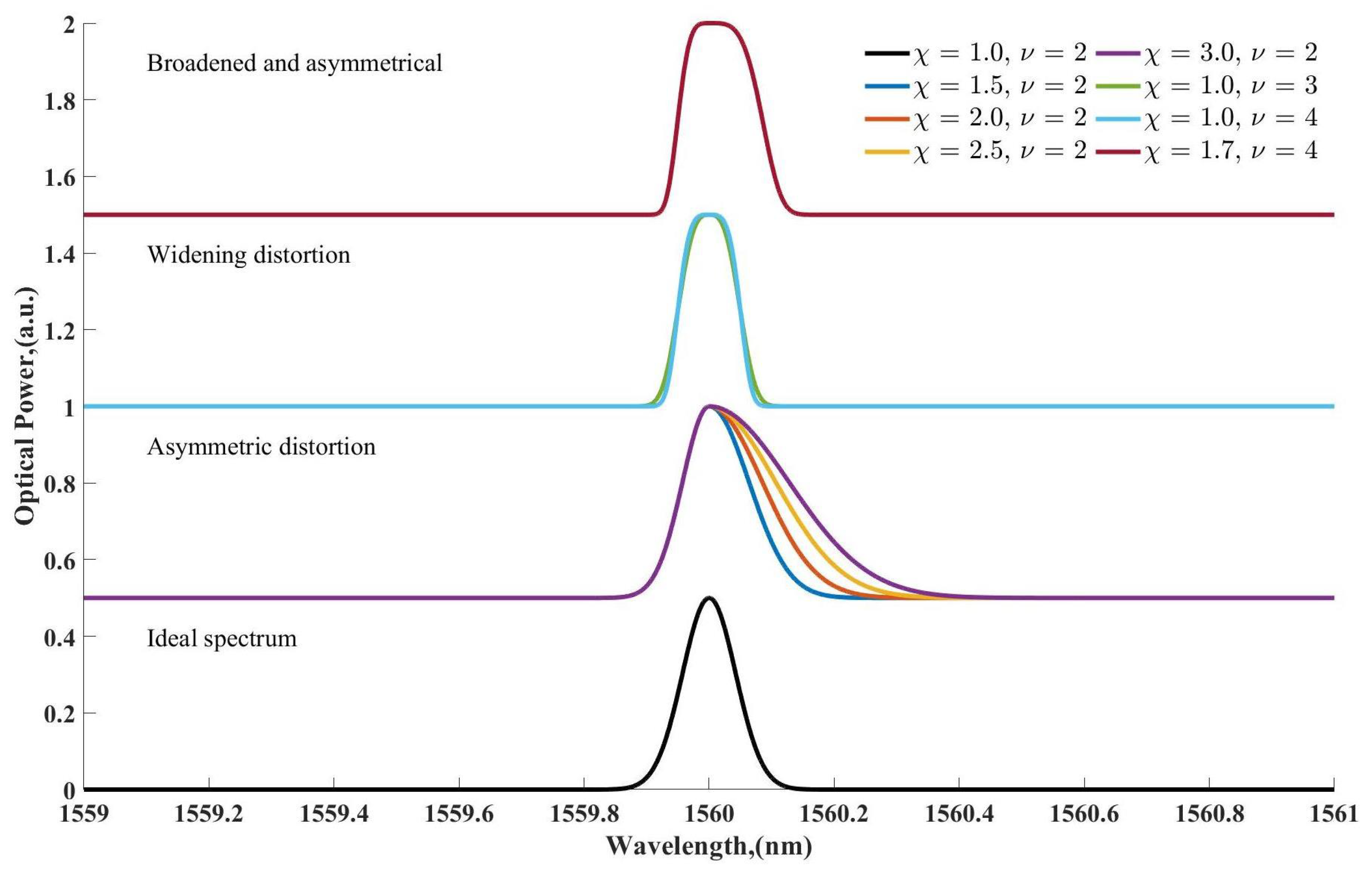
5. K-SVD Denoising Algorithm Based on Adaptive Window Optimization

Let the ideal noise-free FBG spectral signal be $s\left(\lambda \right)$, where the central wavelength ${\lambda }_B$ satisfies the unimodality condition as shown in Equation (9):

$$\left\{\begin{array}{c}{s}^{\prime }\left({\lambda }_B\right)=0\\ s^{″}\left({\lambda }_B\right)<0\end{array}\right.$$

(9)

Within the neighborhood $N({\lambda }_B,\delta )$ around the peak, the number of derivative sign changes $\eta$ characterizes the signal smoothness as Equation (10):

$$\eta (s^{\prime },{\lambda }_B)=\sum _{k=m}^{M-1}∥\left[\mathrm{sgn}\left(s^{\prime }\left({\lambda }_k\right)\right)\ne \mathrm{sgn}\left(s^{\prime }\left({\lambda }_{k+1}\right)\right)\right]=1$$

(10)

where $m=argmin{s}^{\prime }\left(\lambda \right),M=argmax{s}^{\prime }\left(\lambda \right)$ and $∥[·]$ is the indicator function. This condition serves as a necessary and sufficient criterion for the unimodal smoothness of the signal.

The noisy spectral signal can be modeled as Equation (11):

$$y\left(\lambda \right)=s\left(\lambda \right)+n\left(\lambda \right)$$

(11)

where $n\left(\lambda \right)$ represents noise. Its first derivative becomes oscillatory due to noise interference as shown in Equation (12):

$$y\prime \left(\lambda \right)=s\prime \left(\lambda \right)+n\prime \left(\lambda \right)$$

(12)

The noisy derivative $n^{\prime }\left(\lambda \right)$ leads to $\eta (y^{\prime },{\lambda }_B)\ge 2$. By suppressing $n^{\prime }\left(\lambda \right)$, the K-SVD denoising process ensures $\eta ({\widehat{s}}^{\prime },{\lambda }_B)\to 1$, where $\widehat{s}$ is the denoised estimate.

As shown in Figure 2, the number of derivative sign changes $\eta ({\widehat{s}}^{\prime },{\lambda }_B)$ of the denoised noisy simulated signal (SNR = 15 dB, central wavelength = 1560.000 nm) processed by the K-SVD algorithm with varying window sizes L is analyzed. When L is too small, incomplete signal segmentation results in insufficient dictionary representation capability, leading to $\eta ({\widehat{s}}^{\prime },{\lambda }_B)>1$. As L increases, the signal blocks contain more complete waveform features, enabling the dictionary to learn more accurate sparse representations and effectively separate noise. At $L=52$, $\eta ({\widehat{s}}^{\prime },{\lambda }_B)=1$ is achieved. Further increases in L maintain $\eta ({\widehat{s}}^{\prime },{\lambda }_B)\equiv 1$. Figure 3 illustrates the denoising performance of the K-SVD algorithm on the same noisy signal with different L, At $L=22$, poor denoising performance is observed: significant fluctuations near the peak ($\eta ({\widehat{s}}^{\prime },{\lambda }_B)>1$) result in a measured peak wavelength of 1559.989 nm, deviating substantially from the central wavelength. As L increases to 52 (critical point where $\eta ({\widehat{s}}^{\prime },{\lambda }_B)=1$), the denoised peak wavelength matches the central wavelength (1559.000 nm). Beyond $L=52$, although $\eta ({\widehat{s}}^{\prime },{\lambda }_B)\equiv 1$, excessive window sizes cause waveform distortion and peak shift. Thus, the critical window size L at $\eta ({\widehat{s}}^{\prime },{\lambda }_B)=1$ (e.g., $L=52$) ensures optimal performance for the K-SVD algorithm: effective noise suppression while preserving original peak characteristics.

To determine the critical window size, this paper proposes an adaptive window size-based K-SVD algorithm with the following steps:

•  Initialize:
  • Set initial window size $L=1$, step size ${\mathrm{L}}_c=128$.
  • Construct the Hankel matrix $Y\in {\mathbb{R}}^{L\times (N-L+1)}$.
• Apply K-SVD denoising: $\widehat{s}=DX$.
• Compute the number of derivative sign changes $\eta ({\widehat{s}}^{\prime },{\lambda }_B)$.
• Update window size:
  • If $\eta ({\widehat{s}}^{\prime },{\lambda }_B)>1$: $\mathrm{L}=\mathrm{L}+{\mathrm{L}}_c$.
  • Else if $\eta ({\widehat{s}}^{\prime },{\lambda }_B)=1$: $\mathrm{L}=\mathrm{L}-{\mathrm{L}}_c$.
• Adjust step size and iterate:
  • Update ${\mathrm{L}}_c={\mathrm{L}}_c/2$.
  • If ${\mathrm{L}}_c<1$: set ${\mathrm{L}}_c=1$.
  • Terminate if ${\mathrm{L}}_c=1$ and $\eta ({\widehat{s}}^{\prime },{\lambda }_B)=1$.
  • Otherwise, reconstruct the Hankel matrix with updated L and repeat steps 2–5.

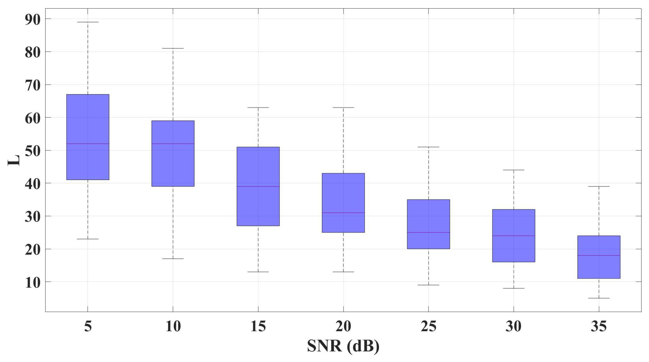
The algorithm aims to rapidly search for an optimal window size L that smooths spectral peaks while eliminating noise-induced spikes. By introducing a variable step size ${\mathrm{L}}_c$ combined with a binary search strategy, the search efficiency is significantly improved. Figure 4 displays the boxplot distribution of window sizes L obtained from 50 consecutive experiments under different SNR conditions. Results show that all optimal L values are below 80. Consequently, ${\mathrm{L}}_c$ is set to 128 (a power of 2) to ensure computational efficiency.

The pseudocode for the SAK-SVD algorithm is presented in Algorithm 1:

Algorithm 1 SAK-SVD algorithm

Require:  FBG reflectance spectral signal y. Ensure:  Optimal window size L, denoised signal $\widehat{s}$.  1: Initialization:  2:    Set window size L, step size $L_c$, dictionary atoms K, max iterations MaxIter.  3:    Construct Hankel matrix $\mathit{Y}$ by segmenting y with window size L. $$Y=\left[\begin{array}{cccc}{y}_1\hfill & y_2& \dots & y_{n^{\prime }}\\ y_2& y_3& \dots & y_{n^{\prime }}+1\\ ⋮& ⋮& ⋮& ⋮\\ y_L& y_{L+1}& \dots & y_n\end{array}\right]$$  4:    Initialize dictionary $\mathit{D}$ by randomly selecting K columns from $\mathit{Y}$.  5: while $\eta ({\widehat{s}}^{\prime },{\lambda }_B)\ne 1$ or $L_c\ne 1$do                    ▹ Main loop  6:     for $\mathrm{Iter}=1$ to MaxIter do       ▹ Sparse coding and dictionary update  7:         Sparse coding: $\mathit{X}=arg{min}_{\mathit{X}}{\parallel \mathit{Y}-\mathit{D}\mathit{X}\parallel }_2^2$  8:         Update $\mathit{D}$ column-wise via SVD.  9:     end for 10:     Denoising: $\widehat{s}=\mathit{D}\mathit{X}$               ▹ Compute denoised signal 11:     Calculate $\eta ({\widehat{s}}^{\prime },{\lambda }_B)$ (derivative sign changes) using Equation (10). 12:     if $\eta ({\widehat{s}}^{\prime },{\lambda }_B)>1$ then             ▹ Adaptive window adjustment 13:         $L=L+L_c$ 14:     else if $\eta ({\widehat{s}}^{\prime },{\lambda }_B)=1$ then 15:         $L=L-L_c$ 16:     end if 17:     $L_c=⌊{\displaystyle \frac{L_c}{2}}⌋$                        ▹ Halve step size 18:     if $L_c<1$ then 19:         $L_c=1$                     ▹ Clamp minimum step size 20:     end if 21:     Rebuild $\mathit{Y}$ and $\mathit{D}$ with new L.                ▹ Matrix reconstruction 22: end while 23: return L, $\widehat{s}$

6. Simulation and Discussion

6.1. Experimental Parameter Design

For the K-SVD algorithm, the dictionary size (defined as $LK$, where L corresponds to the window size of the data and K is the number of atoms in the dictionary) is critical. An excessively large dictionary may introduce redundant atoms, while an overly small dictionary may fail to adequately represent signal features. Thus, the dictionary size must be carefully selected based on signal characteristics and application requirements. 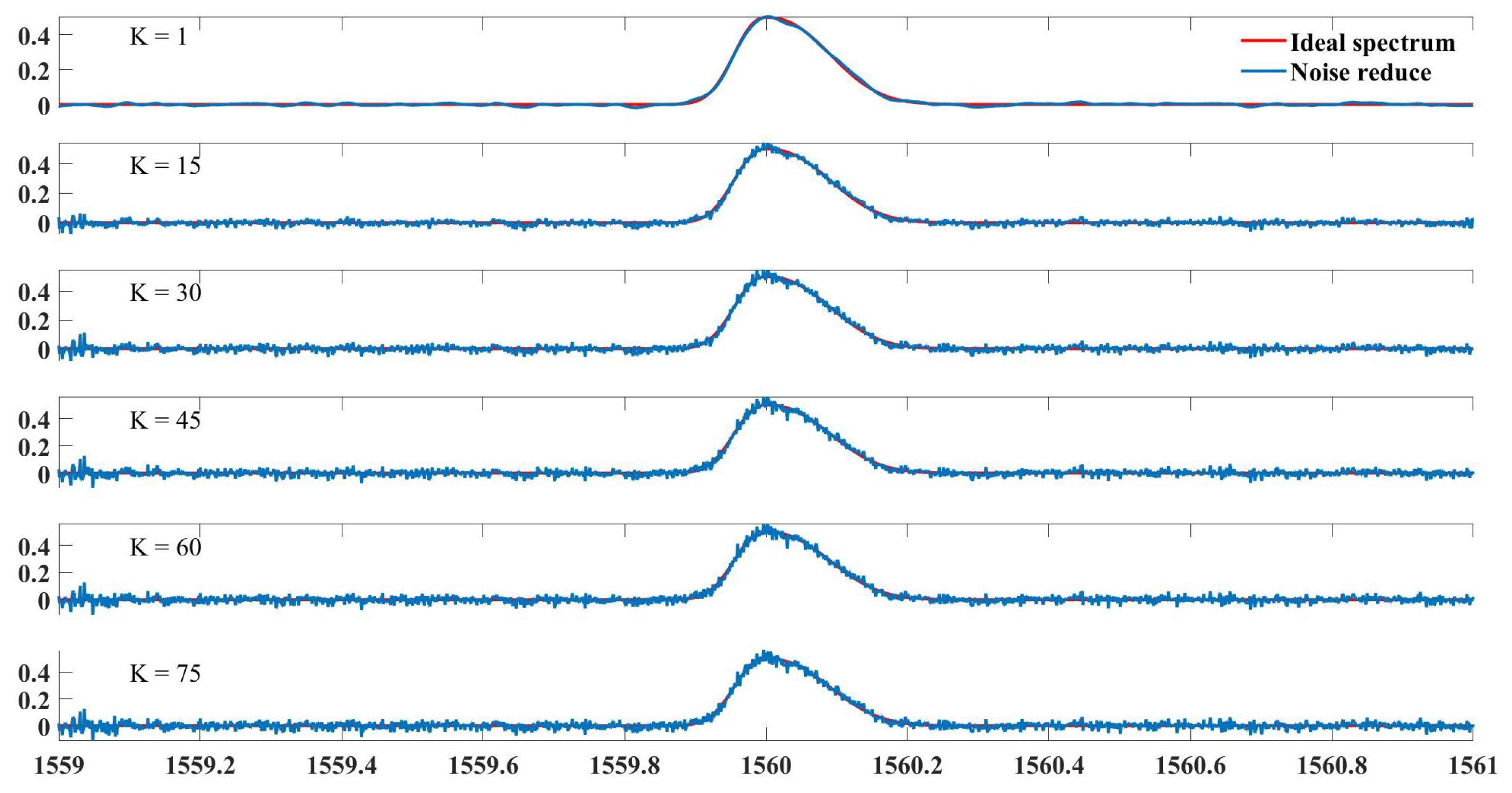Figure 5 compares denoising results under different K. As K increases, the denoised signal exhibits more spurious spikes (glitches). As can be seen from Figure 5, as K gets larger, more noise appears in each spectrum, due to the fact that each iteration of sparse coding in K-SVD denoising fits the residual error. When K exceeds the intrinsic sparsity of the true signal $K^{\ast }$, subsequent atoms inevitably model the noise structure. The experimental results suggest that the FBG spectral signal may exhibit relatively simple structural characteristics, which could be sufficiently represented with a single atom in the sparse domain. Figure 6 shows the SNR between the denoised signal and the original signal for varying K. Larger K values lead to lower SNR. When K is minimized, the denoised signal achieves the highest SNR and minimal waveform distortion, indicating superior denoising efficacy. Consequently, increasing K beyond unity introduces redundant pseudofeatures that degrade denoising performance. Based on this empirical validation, we fix $K=1$ to enforce maximal sparsity while preserving signal fidelity.

In sparse representation, the sparsity level is defined as the number of non-zero coefficients required to represent a signal under a given dictionary. Low sparsity (fewer non-zero coefficients) suppresses noise through strong constraints but may sacrifice fine signal details. High sparsity (more non-zero coefficients) improves reconstruction accuracy. However, an overcomplete dictionary may introduce overfitting due to excessive degrees of freedom. In this experiment, the dictionary size is fixed at $K=1$, thereby constraining the sparsity level to 1.

The K-SVD algorithm iteratively optimizes the solution by alternately updating the dictionary and sparse coefficients. Increasing the number of iterations enhances the convergence of the solution but significantly raises the computational cost, necessitating a trade-off between convergence speed and efficiency. Observing the denoising results by varying the number of iterations, it is experimentally found that as the number of iterations increases from 1, the denoising effect does not improve significantly, and the SNR after denoising remains constant. This may be due to the high sparsity or simple structure of the FBG spectral signal, which is already close to optimum after the first iteration, leading to limited gain in subsequent iterations. Based on these findings, we empirically set the number of iterations to 1 to maximize computational efficiency without compromising accuracy.

6.2. Performance Verification of SAK-SVD with Adaptive L-Parameter for Spectral Signal Denoising

To verify the performance improvement of SAK-SVD over the original algorithm in spectral signal denoising, a controlled experiment is conducted comparing the SAK-SVD algorithm with adaptive L parameter adjustment against the K-SVD algorithm using fixed L parameters. Five control groups with fixed L values (40, 45, 50, 55, 60) are established. The spectral signals are configured with sharpness randomly sampled from 2 to 4, skewness from 1 to 3, central wavelengths spanning 1559–1561 nm, and a fixed SNR of 5 dB. The denoising performance is evaluated using four metrics defined in Equations (13)–(16): the SNR, root mean square error (RMSE), smoothness, cross-correlation, and the peak detection absolute error computed via the direct peak-search method. SNR measures the ratio of effective signal components to noise, where higher values indicate better noise suppression effects. RMSE quantifies the global deviation between the denoised signal and the original noise-free signal, with smaller values reflecting closer alignment to the true signal. Smoothness evaluates the roughness of the denoised signal by averaging the squared differences between adjacent data points. Smaller differences yield lower smoothness values, indicating smoother signals, while larger differences result in higher smoothness values, signifying increased fluctuations. Cross-correlation assesses the structural similarity in the time domain between the denoised and original signals, where values closer to 1 denote stronger trend consistency. All experimental results are averaged over 20 consecutive simulation trials.

$$\mathrm{SNR}=10log[{\displaystyle \frac{{\displaystyle \sum _{i=1}^N}{x}^2\left(i\right)}{{\displaystyle \sum _{i=1}^N}{\left(x\right(i)-y(i\left)\right)}^2}}]$$

(13)

$$RMSE=\sqrt{{\displaystyle \frac{1}{N}}\sum _{i=1}^N{\left(x\right(i)-y(i\left)\right)}^2}$$

(14)

$$smoothness={\displaystyle \frac{{\displaystyle \sum _{i=2}^N}{\left(y\right(i)-y(i-1\left)\right)}^2}{N}}$$

(15)

$$CrossCorrelation={\displaystyle \frac{{\displaystyle \sum _{i=1}^N}(x\left(i\right)-\overline{x})(y\left(i\right)-\overline{y})}{\sqrt{{\displaystyle \sum _{i=1}^N}{(x\left(i\right)-\overline{x})}^2}\times \sqrt{{\displaystyle \sum _{i=1}^N}{(y\left(i\right)-\overline{y})}^2}}}$$

(16)

where x denotes the noisy spectral signal and y represents the denoised spectral signal.

The experimental results are summarized in

Table 1. Comparative results of adaptive and fixed window size K-SVD denoising.

L	SNR (dB)	RMSE	Smoothness	Cross-Correlation	Peak Error (nm)
40	20.7549	0.011033	3.38 × 10−6	0.995798	0.0074
45	19.8012	0.012324	4.06 × 10−6	0.994871	0.01085
50	20.3010	0.011642	3.72 × 10−6	0.995426	0.01005
55	20.72894	0.011089	3.48 × 10−6	0.995851	0.0087
60	21.08735	0.010647	3.30 × 10−6	0.996173	0.0081
Adaptive	21.36902	0.010312	3.17 × 10−6	0.996404	0.0071

. Under the denoising evaluation metric of SNR, the proposed adaptive algorithm achieves the highest SNR of 21.36902 dB, indicating optimal noise suppression capability. For the RMSE metric, the adaptive algorithm yields the lowest RMSE value of 0.010312, demonstrating superior global approximation accuracy to the true signal. In terms of smoothness, the proposed method attains the lowest value of 3.16778 × 10⁻⁶, confirming a smoother denoised signal. The cross-correlation coefficient of the adaptive algorithm reaches 0.996404427 (closest to 1), reflecting the highest consistency in trend between the denoised and original signals. Furthermore, the peak detection absolute error of the adaptive algorithm is minimized at 0.0071 nm, validating the dynamic matching capability between window parameters and signal features. Quantitative analysis reveals that the SAK-SVD algorithm, through dynamic window adjustment, achieves improvements of 1.28% in SNR, 3.05% in RMSE, and 12.35% in peak error compared to the best fixed parameter configuration ($L=60$). These results demonstrate that SAK-SVD effectively balances noise suppression, signal fidelity, and detail preservation while significantly enhancing the denoising performance of the original K-SVD algorithm on spectral signals.

6.3. Comparative Analysis of Adaptive SAK-SVD with FIR, TI-IM, and CEEMDAN-SG for Spectral Signal Denoising

To verify the reliability of SAK-SVD, a comparative simulation experiment was conducted between the SAK-SVD denoising algorithm proposed in this paper and the FIR denoising method, TI-IM denoising method, and CEEMDAN-SG denoising method. These methods were utilized to process random spectral signals with SNR ranging from 5 dB to 35 dB, with a noise increase step of 5 dB. The results of the different methods processing noise at various SNR levels are averaged over 20 consecutive simulation trials. The sharpness $\nu$ of the spectral signals is randomized within the range of 2–4, the skewness $\chi$ is randomized within the range of 1–3, and the central wavelength range is 1559–1561 nm. For the FIR denoising method [17], the sampling frequency is set to 4 MHz, the cutoff frequency of the ideal low-pass filter is 5 kHz, and the filter order is 32. For the TI-IM denoising method [14], sym5 is chosen as the wavelet basis, and six layers of wavelet decomposition are selected. For the CEEMDAN-SG denoising method [19], the noise standard deviation $Nstd$ is set at 0.2, the number of realizations $NR$ is 500, the maximum allowable filtering iterations MaxIter are 5000, the width of the noise filtering sliding window w is 21, and the polynomial fitting order q is 5. The experimental evaluation metrics, consistent with Experiment B, include the SNR, RMSE, smoothness, and cross-correlation.

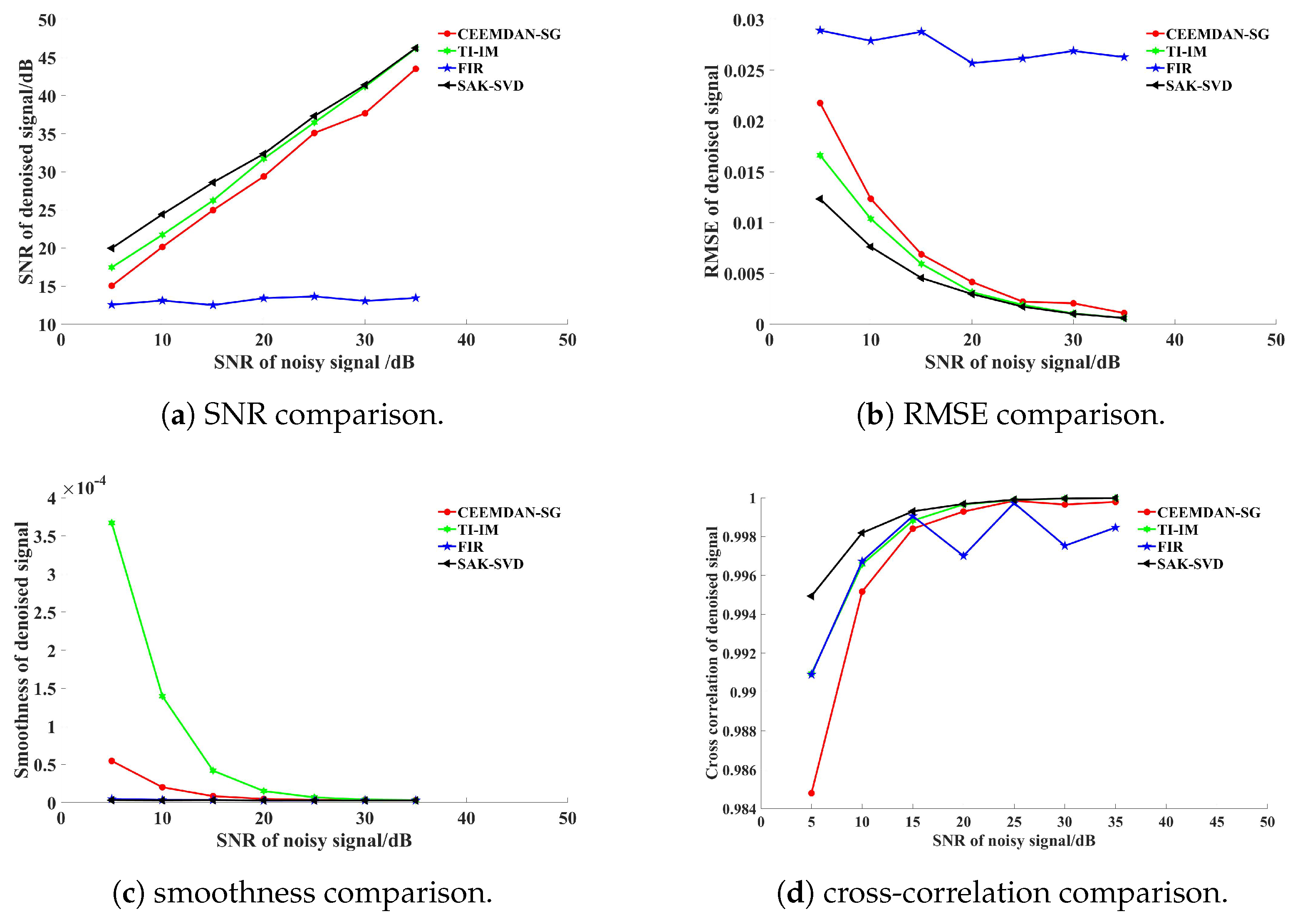
Figure 7 compares the denoising performance of different methods. As shown in Figure 7a, the proposed method achieves the highest SNR after denoising under different noise levels, outperforming all other methods. In Figure 7b, the proposed method yields the lowest RMSE under varying noise levels. Figure 7c demonstrates that the proposed method attains the smallest smoothness value, while Figure 7d shows the cross-correlation coefficient between the denoised signal and the original noise-free signal closest to 1. This result validates exceptional preservation of temporal waveform structures (as defined in Equation (16)). In conclusion, SAK-SVD dominates all metrics—maximizing SNR, minimizing RMSE and smoothness, and achieving cross-correlation coefficients closest to 1—which validates its robustness and comprehensive denoising performance advantages.

6.4. Comparative Analysis of Denoising Algorithms for FBG Wavelength Demodulation Under Noisy and Distorted Conditions

To validate the performance of the proposed method in FBG wavelength demodulation, the simulation waveforms in this experiment were divided into two groups: Group 1 (Undistorted Noisy Waveforms), where distortion parameters are fixed at $\chi =1$ and $\nu =2$, and Group 2 (Randomly Distorted Noisy Waveforms), where $\chi$ was randomly sampled from [1, 3] and $\nu$ was sampled from [2, 4]. Both groups were contaminated with white noise at random SNR levels ranging from 5 dB to 35 dB, with 20 waveforms per group. Four denoising methods (SAK-SVD, FIR, TI-IM, CEEMDAN-SG) were applied to process the waveforms. Subsequently, four demodulation algorithms were implemented on the denoised signals: Direct Peak-searching Method, Centroid Method, Gaussian Fitting Algorithm, and Levenberg–Marquardt (LM) Fitting Algorithm. The absolute wavelength demodulation errors were calculated for each combination, and the final results were averaged over 20 independent trials.

The experimental results are shown in

Table 2. Comparative demodulation results of different denoising algorithms.

Distortion Parameters	Demodulation Method	Absolute Error (pm)
		SAK-SVD	FIR	TI-IM	CEEMDAN-SG
$\chi =1$, $\nu =2$	Direct Peak Search	2.100	15.550	2.500	2.750
	Centroid Method	3.147	5.112	3.164	3.147
	Gaussian Fitting	0.450	14.800	1.750	1.000
	LM Fitting Algorithm	0.300	17.250	0.500	0.400
$\chi =1$–3, $\nu =2$–4	Direct Peak Search	3.900	23.750	12.150	10.650
	Centroid Method	9.786	15.336	9.831	9.826
	Gaussian Fitting	7.450	23.750	10.050	7.550
	LM Fitting Algorithm	7.500	22.850	7.650	7.500

. From the table, it can be seen that in the undistorted waveform experiments, for each demodulation algorithm, the use of the SAK-SVD algorithm for waveform denoising reduced the absolute demodulation errors. Specifically, under undistorted conditions, SAK-SVD achieved an LM fitting error of 0.3 pm, representing a 25% reduction compared to the suboptimal method (CEEMDAN-SG), and an average error reduction of 32.5% across all demodulation algorithms. In the distorted waveform experiments, the demodulation errors of all algorithms increased, but the errors using the SAK-SVD denoising algorithm remained relatively lower. Notably, for the direct peak-searching method, SAK-SVD reduced the error from 10.650 pm (suboptimal method: CEEMDAN-SG) to 3.900 pm under distorted conditions—an optimization of 63.38%, proving its strong adaptability to waveform distortion. The error escalation factor of SAK-SVD under distorted conditions averaged 11.66 times, significantly lower than other methods (FIR: 24.7 times, TI-IM: 18.2 times, CEEMDAN-SG: 15.4 times), validating the effectiveness of its dynamic parameter adaptation mechanism.

The experiments conducted clearly demonstrate that the proposed denoising algorithm effectively preserves original features while simultaneously suppressing noise, thereby enhancing demodulation accuracy. The optimal mean absolute error for denoising undistorted waveforms is 0.300 pm, while for distorted waveforms, it reaches 3.9 pm.

7. Conclusions

This paper proposes a self-adaptive K-SVD algorithm to enhance the denoising performance of the K-SVD algorithm on spectral signals. The proposed algorithm dynamically adjusts the window size based on the denoising results of different spectral signals to achieve optimal performance. Experimental results demonstrate that compared to FIR filtering, CEEMDAN-SG, and wavelet threshold denoising, the improved SAK-SVD method achieves superior performance across all four evaluation metrics: SNR, RMSE, smoothness, and cross-correlation coefficient. Furthermore, the proposed algorithm enhances the demodulation accuracy of direct peak-searching, centroid method, Gaussian fitting, and LM fitting algorithms. For undistorted waveforms, it achieves a minimum mean absolute error of 0.3 pm, while for distorted waveforms, the MAE is 3.9 pm—the lowest among all four denoising methods. Critically, these advancements directly enhance FBG sensing systems in key industrial applications: structural health monitoring (SHM) of infrastructure (e.g., bridges, dams), enabling subpicometer strain resolution for early crack detection; real-time equipment diagnostics in high-precision manufacturing (e.g., turbine blade deformation tracking); and aerospace structural integrity monitoring. Beyond optics, the SAK-SVD framework provides a novel solution for one-dimensional signal denoising, with potential extensions to acoustic emission analysis in mechanical systems, biomedical signal processing (e.g., ECG/EEG artifact removal), and vibration signature extraction from rotating machinery. Notably, three limitations of the current SAK-SVD algorithm should be acknowledged: (1) Suboptimal asymmetric distortion handling: When processing spectra with severe asymmetric distortion (e.g., non-uniform strain fields in composite materials or near structural discontinuities), the model shows limited ability in peak-shape recovery, constraining further improvements in demodulation accuracy beyond the observed 3.9 pm MAE; (2) Single-peak spectral constraint: This method is currently ineffective for multipeak FBG spectra (e.g., overlapping sensor arrays or complex gratings), as its dictionary learning framework relies on localized single-peak priors; (3) Increased computational cost: The dual-iteration mechanism (alternating between window-size optimization and dictionary learning) significantly increases the computational time compared to simpler denoising methods, potentially limiting its applicability in scenarios demanding real-time, high-frequency demodulation (e.g., vibration monitoring > 1 kHz) or resource-constrained embedded systems. Future work will focus on adapting SAK-SVD to multipeak FBG spectra and deploying it on real-time embedded systems.