Abstract
Spectral computed tomography (SCT) enables material decomposition, artifact reduction, and contrast enhancement, leveraging symmetry principles across its technical framework to enhance material differentiation and image quality. However, its nonlinear data acquisition process involving noise and scatter leads to a highly ill-posed inverse problem. To address this, we propose a dual-domain iterative reconstruction network that combines joint learning reconstruction with physical process modeling, which also uses the symmetric complementary properties of the two domains for optimization. A dedicated physical module models the SCT forward process to ensure stability and accuracy, while a residual-to-residual strategy reduces the computational burden of model-based iterative reconstruction (MBIR). Our method, which won the AAPM DL-Spectral CT Challenge, achieves high-accuracy material decomposition. Extensive evaluations also demonstrate its robustness under varying noise levels, confirming the method’s generalizability. This integrated approach effectively combines the strengths of physical modeling, MBIR, and deep learning.
1. Introduction
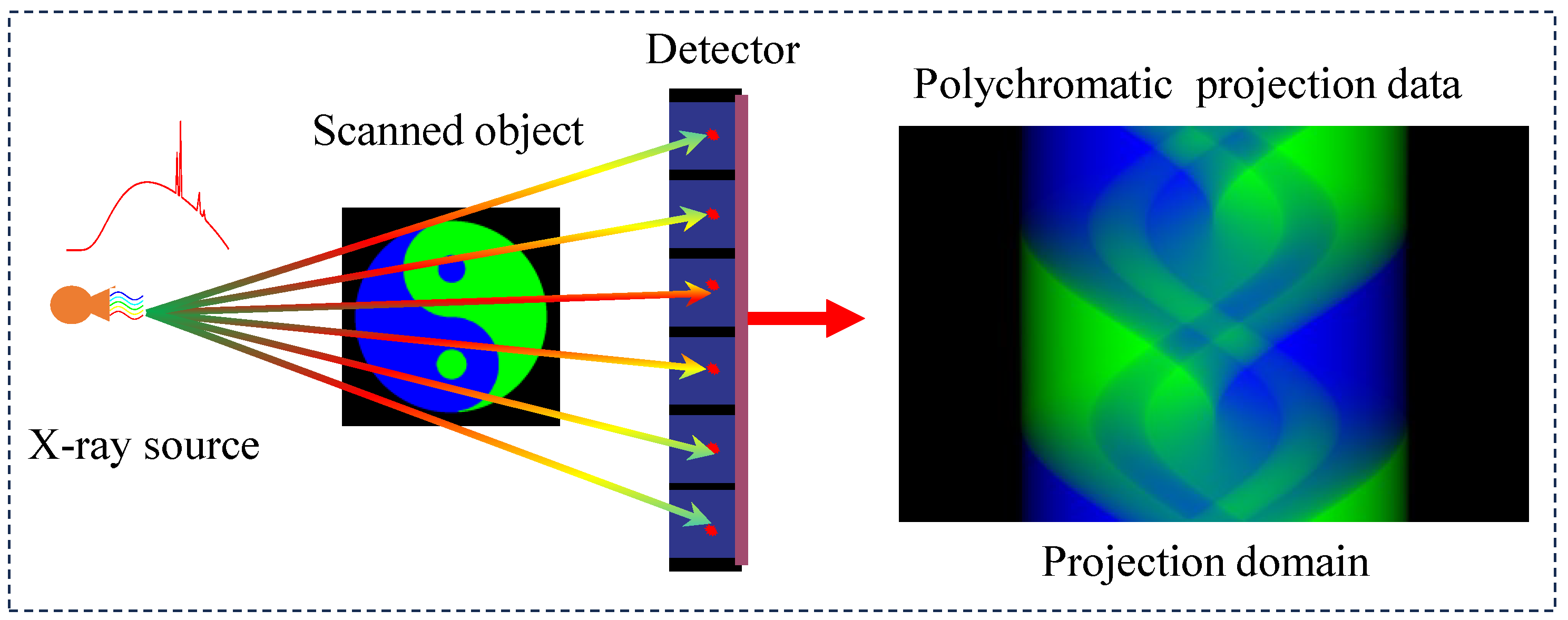
Spectral computed tomography (SCT) has emerged as a pivotal imaging modality with growing applications in clinical diagnostics and industrial nondestructive testing. Unlike conventional CT systems (illustrated in Figure 1), which focus on reconstructing precise anatomical images through multi-angle scanning, SCT fundamentally addresses the critical yet often overlooked polychromatic nature of X-ray beams. This inherent spectral broadening phenomenon introduces nonlinear effects and ill-posed challenges in quantitative imaging reconstruction. The paradigm shift in SCT implementation involves strategic spectral differentiation through two primary approaches: (1) multi-spectral scanning using varied X-ray spectra, or (2) spectral separation from broad-spectrum emissions. Current spectral data acquisition methodologies encompass (1) kVp-switching techniques [1], (2) dual-source scanning systems [2], (3) dual-layer detector configurations, (4) sequential two-pass scanning protocols, and (5) photon-counting detectors [3,4]. These technological advancements have enabled sophisticated processing of polychromatic projection data, facilitating energy-resolved material decomposition through established algorithms [5,6,7,8]. The clinical significance of SCT lies in its dual capability; enhanced material discriminability through spectral signatures and precise quantification of mass density ratios in multi-component systems are particularly beneficial for tissue analysis and composite material characterization [9].
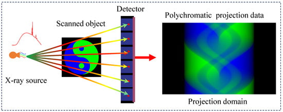
Figure 1.
Spectral computed tomography imaging process.
Compared to conventional CT systems, the reconstruction challenges in spectral computed tomography (SCT) demonstrate inherent nonlinearity and ill-posedness stemming from the subtle spectral differences during spectral separation, further exacerbated by potential geometric inconsistencies in real projection data. Current algorithmic approaches to address these challenges can be systematically classified using two taxonomies: (1) in the processing domain, methods are divided into image domain approaches [8,9,10,11,12,13,14] and projection domain methods [15,16]; (2) among decomposition strategies, methods can be categorized as direct mapping methods [5,10,11,12,13,14,15,17,18,19], iterative algorithms [16,20,21,22,23,24,25,26,27,28,29,30,31,32,33], or deep learning methods [34,35,36,37,38,39,40,41,42].
While image domain methods utilize diverse basis functions [10,11,15,18] to approximate nonlinear effects, they are fundamentally constrained by first-order linear assumptions, leading to persistent beam-hardening artifacts. Projection domain approaches theoretically allow for superior artifact suppression through nonlinear material decomposition [43,44]; however, they demand stringent geometric consistency that is rarely achievable in practical SCT implementations. Direct mapping techniques prioritize computational efficiency while compromising spectral information and exhibiting phantom-dependent accuracy. Iterative algorithms, including one-step spectral CT reconstruction approaches [32,33], are effective for ill-posed inverse problems; however, they confront computational bottlenecks in handling multi-spectral geometric inconsistencies and hyperparameter tuning challenges [45]. Deep learning methods achieve remarkable reconstruction quality given sufficient training data, but struggle with clinical data acquisition limitations and generalizability issues. The AAPM DL-Spectral CT Challenge [46] provides a critical benchmarking platform comparing data-driven and iterative approaches in terms of their ability to address spectral CT’s incomplete measurement problem, thereby promoting methodological advancements through standardized assessment.
This study examines whether deep neural networks can achieve accurate material-specific image decomposition to establish the foundation for data-driven deep learning-based SCT reconstruction algorithms [45]. We propose a novel iterative network architecture that integrates SCT physical modeling with model-based iterative reconstruction (MBIR) algorithms. Although the AAPM Challenge provides detailed physical processes (complete spectral and attenuation coefficient information), our approach reformulates the physical process and its associated parameters as learnable network components for enhanced flexibility. Following the sparse-view CT methodology within DL [47], high-accuracy reconstruction requires explicit incorporation of the forward model within the reconstruction framework, as demonstrated by iterative data consistency optimization. The proposed framework embeds physical processes via physics-constrained modules to enable precise forward modeling during iterative steps, ensuring correct residual propagation. For clinical noisy data, we implement adaptive regularization strategies to improve practical applicability. Our code is publicly available at JLRM code: https://github.com/GM0322/JLRM (accessed on 10 November 2024).
2. Preliminary Knowledge
The mathematical formulation of the SCT problem can be expressed as solving for from K sets of polychromatic projection data under distinct spectra:
where L denotes an X-ray projection path, represents the linear attenuation coefficient at spatial position with energy E, and , is the normalized effective spectrum satisfying . The perturbation term accounts for scatter/noise effects. The linear attenuation coefficient in SCT is typically decomposed as a linear combination of some predefined basis functions
where are energy-dependent coefficients and correspond to spatial distributions. Symmetry here ensures complete spectral coverage, enabling quantitative analysis. This formulation has dual physical interpretations. (1) Physical effect decomposition: for with basis functions derived from photoelectric and Compton scattering effects [5,6], we have (photoelectric) and (Klein-Nishina function); then, and respectively indicate the photoelectric part and Compton scattering part of the attenuation. The reconstructed respectively quantify the spatial distributions of these effects, enabling computation of electron density and effective atomic number. (2) Basis material decomposition: are interpreted as mass attenuation coefficients of selected basis materials, while represent the corresponding material density distributions, with M specifying the number of basis materials.
3. Method
3.1. JLRM Architecture
We formulate SCT reconstruction as a nonlinear optimization problem to solve basis material images from acquired polychromatic projections :
where corresponds to the nonlinear SCT physical process and and are network regularization terms in the projection and image domains, respectively, used in case of noise or scattering. In this way, can more accurately describe the physical model for cases with noise or scattering, as can effectively suppress the noise or scattering to obtain better reconstructed images.
Here, we adopt a simple alternating minimization [48,49] and incremental learning technique [50] to solve (5). Let denote the solution after the th iteration; then, can be obtained by solving the following two subproblems sequentially:
Subproblem 1: Projection domain
Subproblem 2: Image domain
For Subproblem 1, under noise-free conditions, the minimization of is implemented through a network architecture that exclusively contains the physical process module (as detailed in Section 3.1.1). When both the spectral information and attenuation coefficients are unknown, the trainable parameters in this network correspond to these spectral and attenuation components. Notably, when the spectrum is known or fixed, this network module becomes non-trainable with no learnable parameters, and this part does not require training. In noisy scenarios, the optimization comprises two components: (1) the physics-based forward module, and (2) a neural regularization item that suppresses noise and scattering artifacts in the projections generated by the physical module. To achieve noise suppression, we design an iterative network architecture in which the input first generates through physical modeling, which is then processed by a neural module to produce refined projections. These neural-processed results undergo weighted summation with the original to yield :
The final loss function computes the mean squared error (MSE) between the enhanced projection and the clean reference:
with representing the ground truth, where for the noise-free case. In summary, the projection domain optimization process combining physical modeling and neural regularization can be formally expressed as follows:
For Subproblem 2, the same optimization framework could theoretically be applied; however, empirical studies revealed that this sequential approach suffers from catastrophic forgetting in which previously corrected material decompositions tend to regress in subsequent iterations. To address this limitation, we implement a continual learning paradigm with incremental learning retention [51]:
where the incremental update is governed by the dual components shown below.
For the data fidelity pathway, this dual-pathway architecture features a combination of model-based iterative reconstruction with decomposition networks. This is expressed as (, where is used to realize the decomposition of increments in the image domain; this part corresponds to our residual-to-residual learning strategy. The second pathway consists of regularization to further adaptively optimize noisy data.
In summary, the optimization problem can be decomposed into the following four steps:
- Step 1. Obtain initial value:
- Step 2. Nonlinear physical process:
- Step 3. Residual increment: CNN(MBIR
- Step 4. Update: .
In our experiments, the MBIR uses the SART algorithm during the iteration process, which the other algorithm also support. The third step is worth noting; fe first calculate the projection residuals for reconstruction, then the results are input to the CNN to obtain the residuals of the base material images. In other words, we use s residual-to-residual strategy for network training, which can more effectively improve the image quality. In addition, it is important to note that the regularization term needs to be designed to make the method more suitable for situations with noisy data or scattering. For noise-free data, it is not necessary to use the regularization term.
Generally, the initial value has a pronounced influence on the convergence speed of the iterative algorithm; therefore, we incorporate a pre-decomposition module prior to the iterative process.
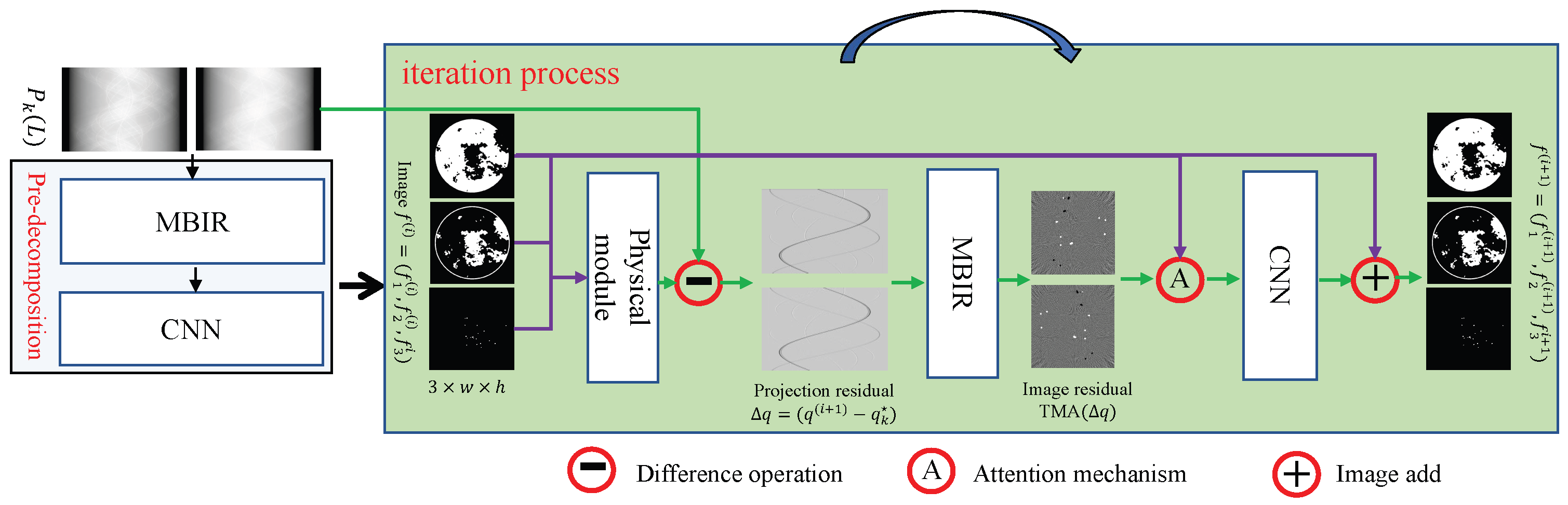
Our architecture integrates a spectral pre-decomposition module and an iterative reconstruction workflow, as visualized in Figure 2 under noise-free conditions. The pre-decomposition stage employs a hybrid MBIR-CNN pipeline, where the E-ART algorithm—notable for its spectral insensitivity and superior reconstruction fidelity compared to conventional analytical methods—provides robust initialization. For the iterative process, the three steps of the incremental method are consistent. As mentioned above, we use a residual-to-residual strategy for effective network training. Below, we show the pseudocode for the training stage (Algorithm 1) and test stage (Algorithm 2).
| Algorithm 1 Training stage |
|
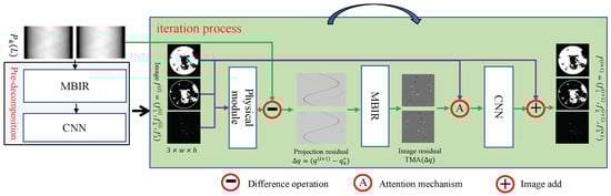
Figure 2.
Architecture of the proposed method, including pre-decomposition module and iteration process.
| Algorithm 2 Test stage |
|
The proposed method is based on the complementary advantages of physical processing, MBIR, and deep learning. Physical processing realizes the accurate expression of physical phenomena, MBIRs achieve domain transformation, and deep learning can accurately perform material decomposition. The three parts are interdependent and complementary.
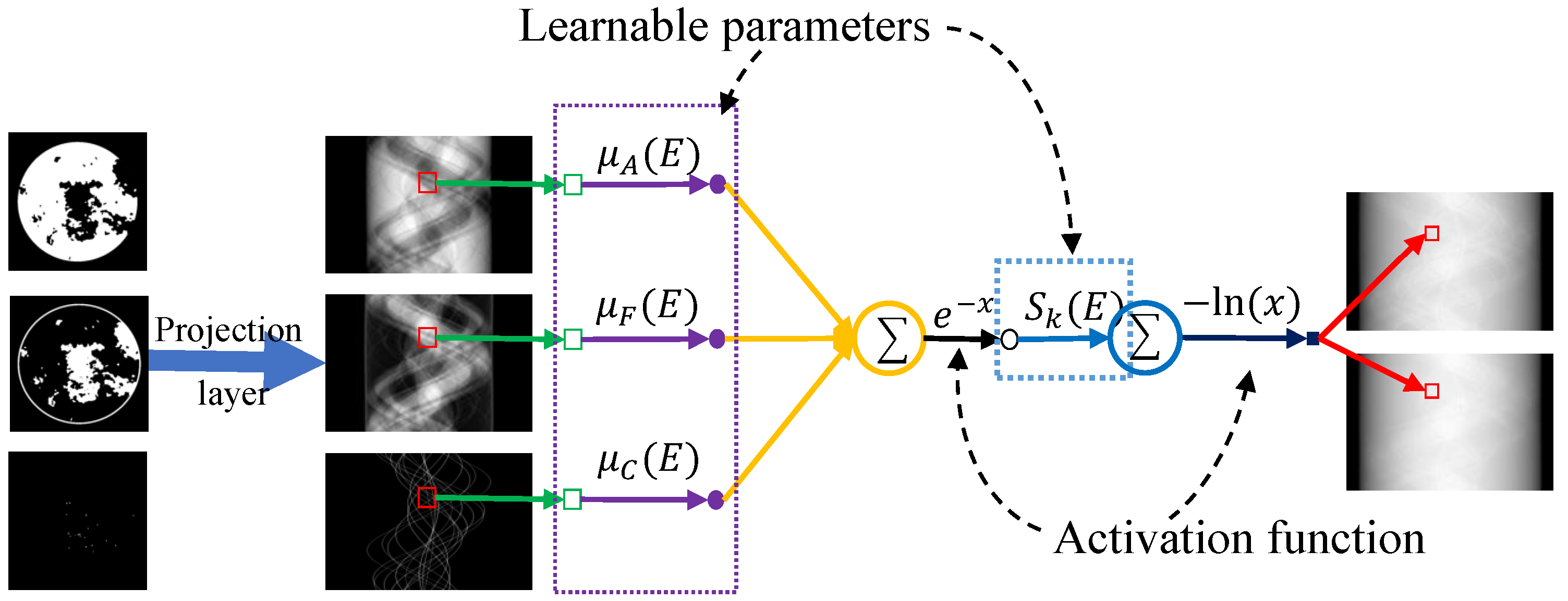
3.1.1. Physical Module for Nonlinear Physical Process
Only when the physical process can be accurately described by the model can the iterative reconstruction process continuously improve reconstruction accuracy. Here, to accurately describe the nonlinear physical process of SCT, its forward process is equivalently mapped into a network module. For noise-free cases, the discrete formulation of SCT can be expressed as Equation (4). As shown in Figure 3, we first perform a Radon transform for three basis materials. This can be achieved by a projection layer [52,53]. Here, we have overridden the interface where projection and back-projection operators are provided by the official framework. Next, the module is constructed according to the discrete polychromatic projection formula, where the spectral information and attenuation coefficients are defined as learnable parameters. Both sets of parameters are implemented through convolution operators. For the attenuation coefficients, this layer uses K convolution kernels with dimensions (). For spectral information, the K convolution kernels have dimensions . In noisy scenarios, a regularization network is added to the physical module to better model the physical process. It should be noted that because the competition provides the energy spectrum information, we do not update it after initialization during the network process.
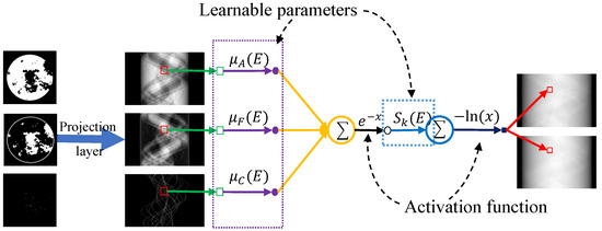
Figure 3.
Physical process equivalent mapping physical module.
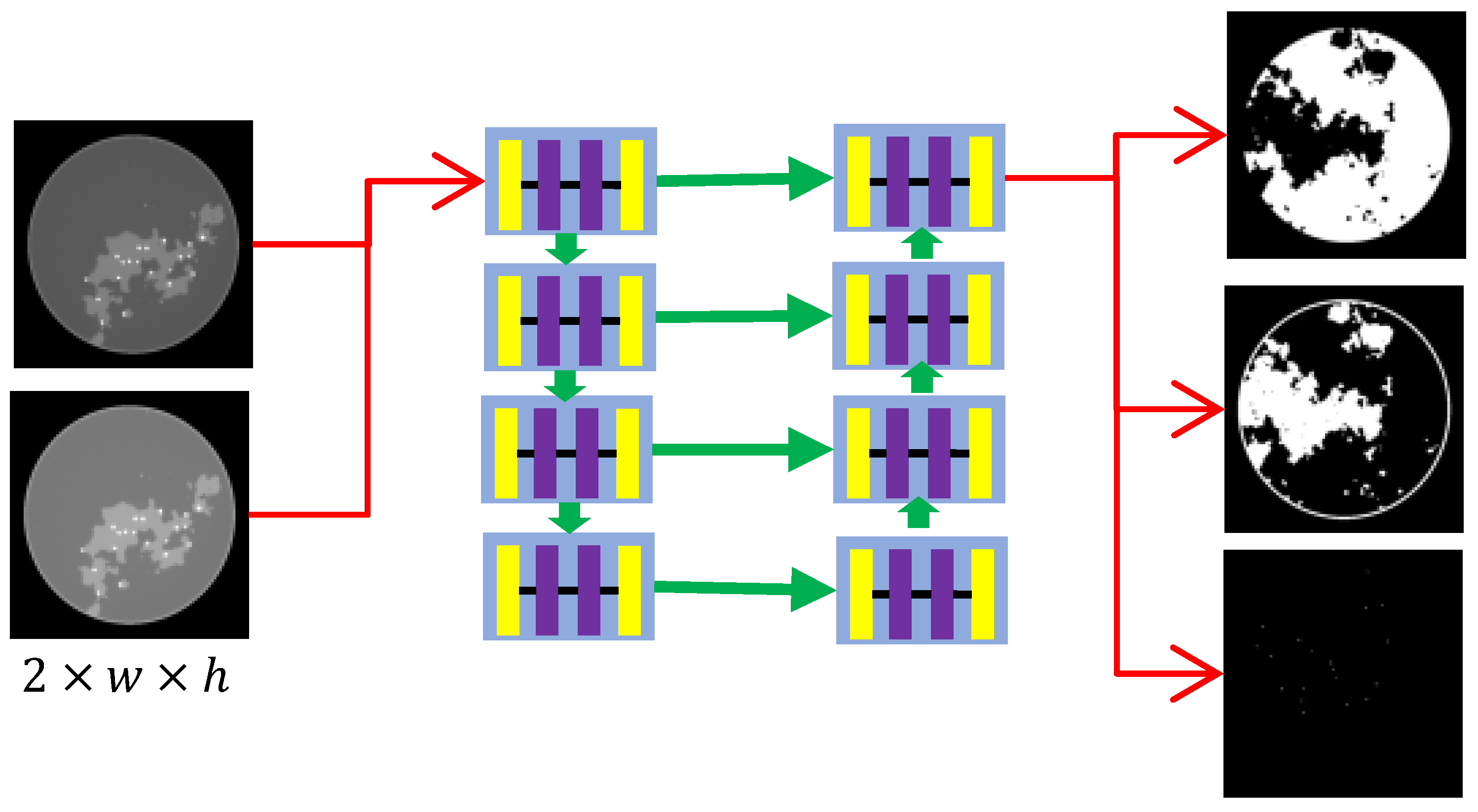
3.1.2. CNN Network Structure Design
The network structure is also critical to the reconstruction results, since our network is trained module-to-module. If overfitting occurs, the results of subsequent iterations are disastrous. The CNNs for the pre-decomposition and iterative processes are structurally similar, with architectures as displayed in Figure 4. The biggest difference between them lies in the input channel configuration: CNN1 uses two input channels, whereas CNN2 employs six channels. Specifically, the CNN can be regarded as two segments. The left branch of the CNN architecture includes four blocks forming a stacked encoder, which implements a sequence of convolution, group normalization (GN), and ReLU activation layers. Given the input x and output y of one block, this process can be expressed as
where are convolutional layers with kernel sizes of , and , respectively. The right branch of the CNN architecture includes four blocks as a stacked decoder. For each block, we first concatenate the feature map of the corresponding block on the left to achieve information fusion. Defining the last output as x, the output of the left branch as , and the output as y, then . A convolutional block identical to the stacked encoder is then applied.
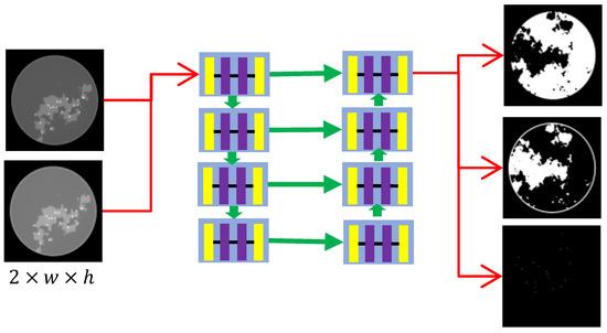
Figure 4.
CNN network structure with eight blocks, each with three convolution layers.
It is worth noting that network operations such as downsampling, upsampling, and transpose convolution—which enlarge the receptive field—cannot be used. Although the projections are inconsistent and the pixels of basis material images exhibit domain-specific correlations, the spatial coherence caused by projection inconsistency is inherently limited. Enlarging the receptive field would exacerbate overfitting, a critical flaw that severely undermines the ability of subsequent iterations to achieve accurate material decomposition.
3.1.3. Residual-to-Residual Strategy
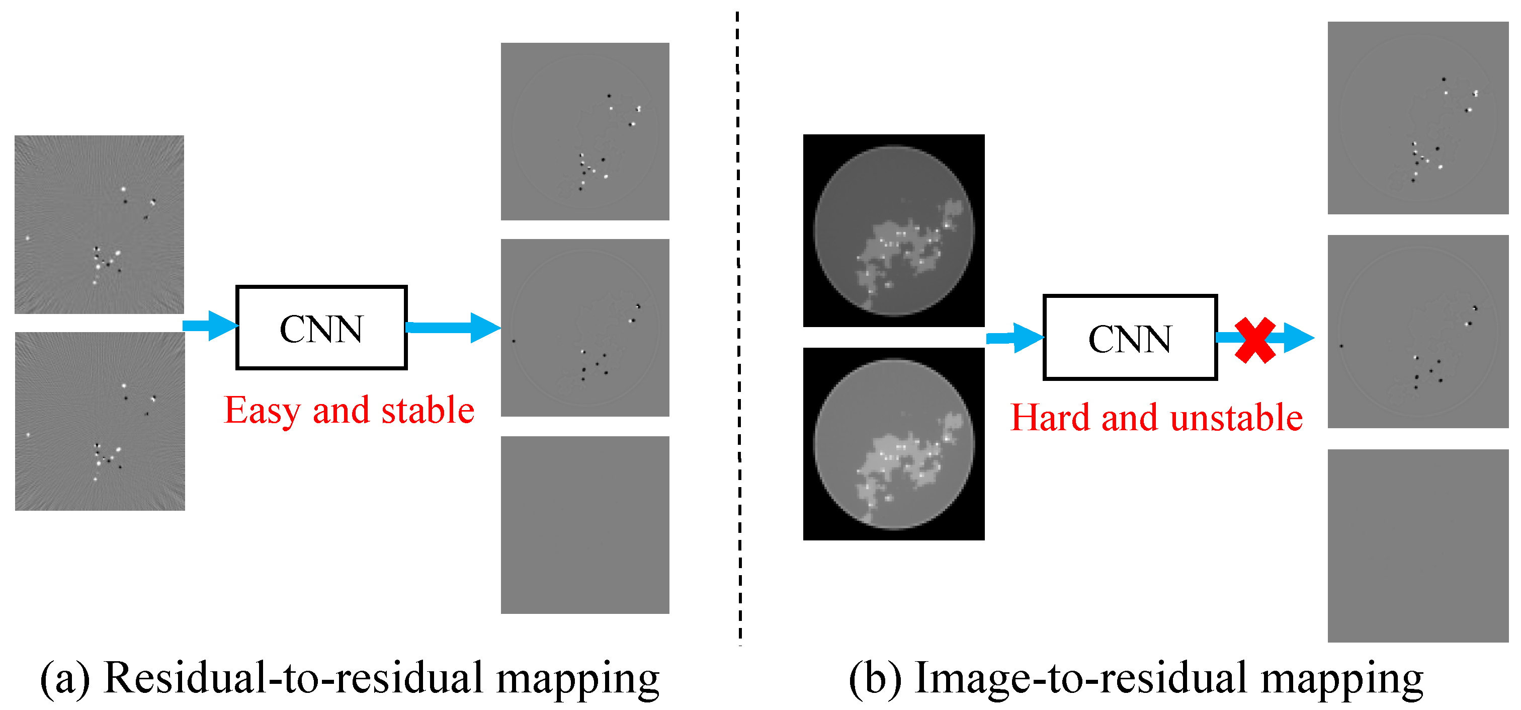
Based on the input and output images of our network, we can define training strategies such as residual-to-image, image-to-image, and others. For example, when the input is an image reconstructed from projection data and the output is the residual of basis material images, we define this as an image-to-image strategy; similarly, when the input is the residual of projection data reconstruction and the output is the residual of basis material images, we define this as a residual-to-residual training strategy.
The residual-to-residual strategy proposed based on experimental observations can effectively improve the accuracy of the reconstruction. As shown in Figure 5, regions with large errors which are difficult to identify in reconstructed images can be directly located in the residual image. Hence, the image-to-residual strategy may introduce new errors, introducing uncertainties that hinder quality improvement of reconstructed images; in other words, image-to-residual is less reliable for improving the image quality.
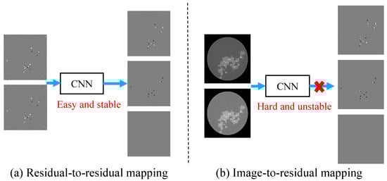
Figure 5.
Residual-to-residual vs. image-to-residual strategy. The residual-to-residual strategy makes it easier to locate large errors.
The commonly used ReLU activation function makes the images obtained by the network non-negative if the last layer of network uses the ReLU function. However, the residual image does not possess this property. In order to use the nonlinear ReLU activation function, we decompose the residual image into the following form:
where and are the positive and negative parts of the residual image, respectively. Thus, the network output becomes an image with two non-negative channels.
3.2. Network Training
The proposed method was implemented using Python (version 3.9) under the PyTorch (version 2.3) framework. Each module was trained module-by-module, and the network was optimized using the Adam optimization method with for each iteration. In order to make the network more generalizable, we used the method of rotation, translation, and mirroring to enhance the data. At the same time, we used a single learning rate (lr = 1 × 10⁻⁴) for learning. The objective function for each module used an MSE loss function:
where are the input/label data, denotes the network learnable parameters, and i is the traversal of the image. The complete training samples were randomly shuffled and the number of training epochs was set to 1000 as an empirical stopping criterion of each module. Comparative experiments were performed on a PC (AMD EPYC-Rome processor, Taichung, Taiwan/CN 128 GB RAM). Training was executed on a single-GPU Nvidia RTX A6000 (Santa Clara, CA, USA) with 48 GB of video memory.
We specifically emphasize the module-by-module training strategy, in which each component is independently parameterized. Below, we list the inputs and output of each module.
Pre-decomposition phase:
- Input: EART-decomposed basis material images
- Processing: Three dedicated networks individually process the inputs
- Output: Refined images of three basis materials
Physical Module:
- Condition: Activated when spectral information is unknown
- Input: Polychromatic projection data paired with reference labels
- Function: Updates the spectral information through physics-constrained learning
Residual-to-Residual Module:
- Input: Reconstructed images from projection residual and current basis material images
- Processing: Three separate networks generate material-specific residuals
- Output: Corrected residual images for each basis material
It is worth noting that all modules undergo isolated parameter updates without cross-module gradient interference.
4. Results
Experiments were carried out to demonstrate the behavior of the proposed method, including architecture validation, residual analysis, the performance of JLRM in noise suppression, the reconstruction method, the CNN network structure design, and the residual-to-residual strategy.
4.1. DL-Spectral CT Setup of AAPM Challenge
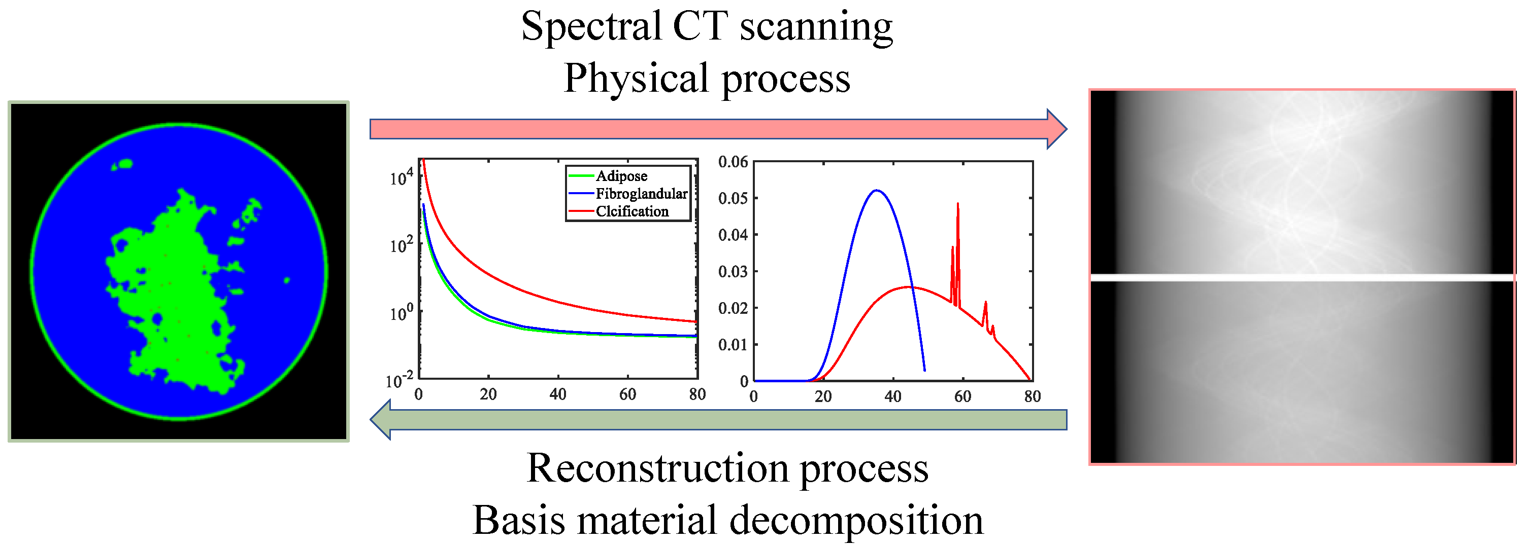
This challenge focuses on spectral CT, in which objects are scanned using X-rays with two spectra (i.e., ) under noise-free conditions. This challenge models an idealized form of fast kVp-switching, where the X-ray tube voltage alternates between two settings for consecutive projections. For each kVp setting, the beam spectrum is broad, and the polychromatic nature of the X-ray beam makes quantitative CT imaging particularly challenging when only one kVp setting is used. Scanned objects are simulated based on a breast model [54], which contains three tissue types (): adipose, fibroglandular, and calcification. Ground truth images and simulated data are provided for 1000 cases, enabling participants to choose between data-driven or optimization-based techniques. The SCT imaging process is illustrated in Figure 6, which shows the spectral information and material-specific linear attenuation coefficients. Notably, the linear attenuation coefficients of the two materials are very close, a key challenge discussed in the experimental results. To ensure fairness, the test dataset includes ten additional cases provided in a “starting kit” with ground-truth images. The fan-beam geometric parameters of the SCT system are listed in Table 1. The DL-Spectral-CT Challenge aims to identify the image reconstruction algorithm that achieves the most accurate spatial maps of adipose, fibroglandular, and calcification from SCT projection data. Further details about the challenge setup and results are available in the official report [46].
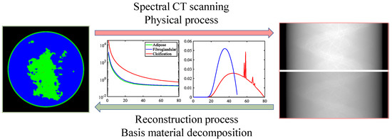
Figure 6.
SCT imaging. The forward process is data collection, which is also a physical process. The inverse process is reconstruction, i.e., basis material decomposition.

Table 1.
System and geometric scanning parameters of the AAPM DL-Spectral CT Challenge dataset.
4.2. Performance and Analysis of JLRM
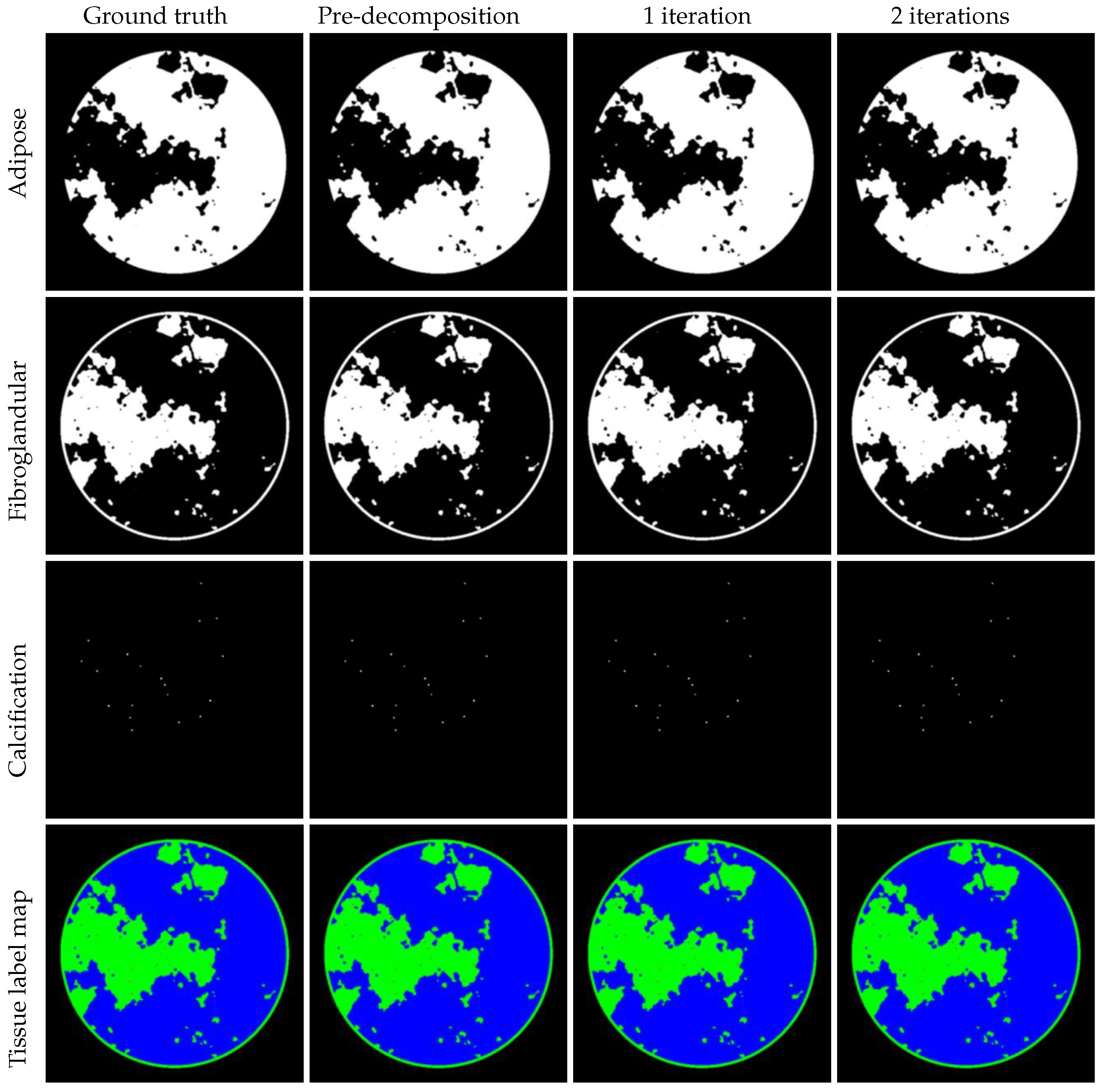
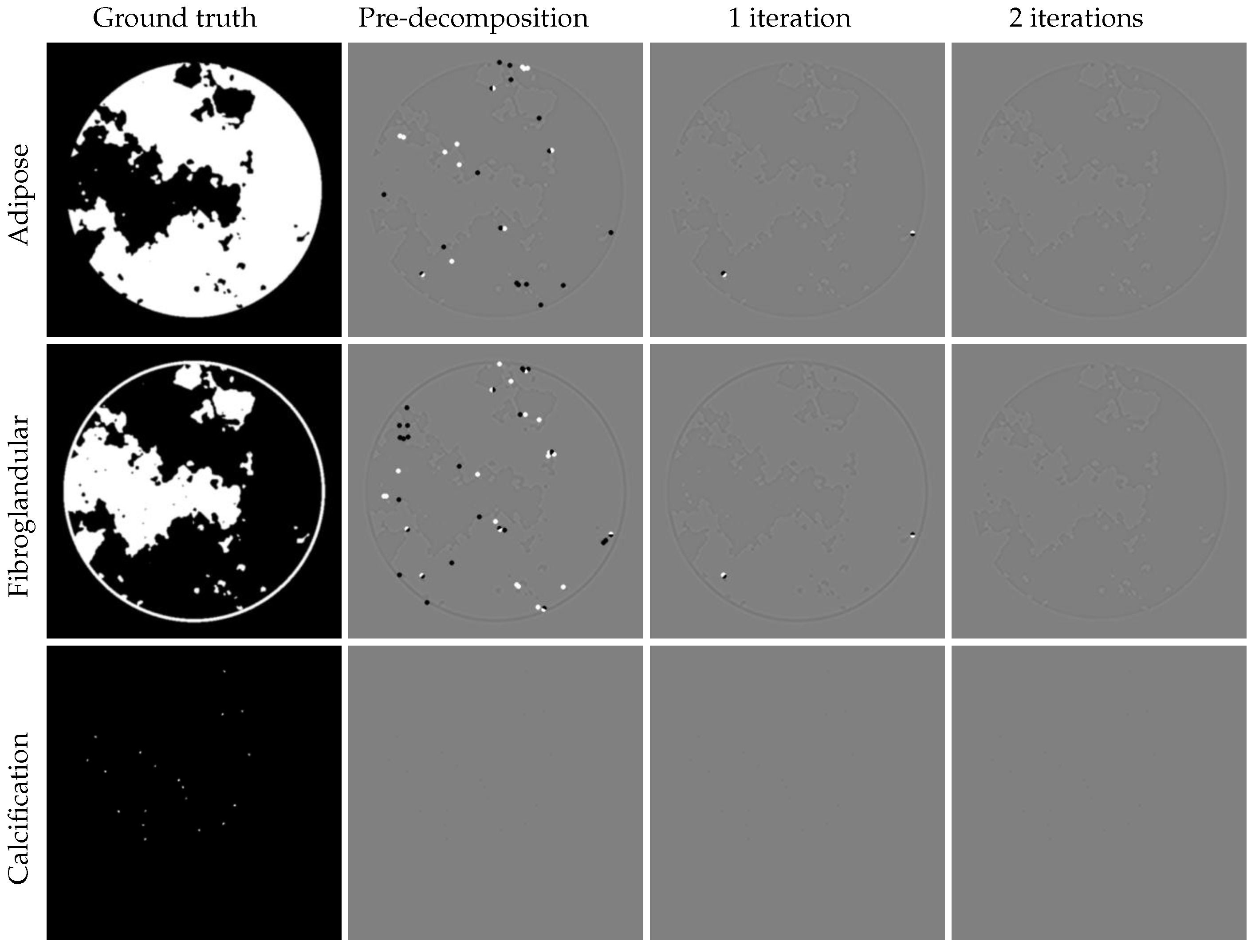
We demonstrate that JLRM can be trained to accurately reconstruct basis material images from collected projection data in the DL-Spectral CT Challenge dataset. As described in Section 3, the JLRM method includes a pre-decomposition module and two iterative refinement modules. Figure 7 shows the basis material images these three modules. It is difficult to visually distinguish the image quality produced by each module. The last row displays the tissue label map of the three materials, revealing the proportion of each material per pixel. Figure 8 shows the difference images. The accuracy of the proposed method can be further improved, as the iterative modules continuously enhance reconstruction quality through comparison with differential images. Even in a display window approaching machine precision, the difference images after two iterations show negligible errors, validating the near-exact reconstruction capability of our method. Table 2 provides the average RMSE for quantitative evaluation, confirming the accuracy of our reconstruction. The final submitted result in the AAPM challenge achieved an accuracy of —approaching the single-precision floating-point limit (∼). Compared to the second-place accuracy (), our method demonstrates an order-of-magnitude improvement.
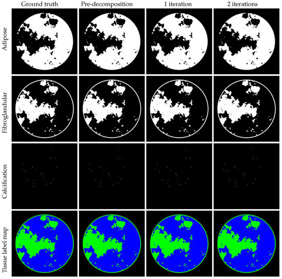
Figure 7.
Left to right: ground truth, results of pre-decomposition block, iteration process with one and two iterations. Display windows: for adipose material, for fibroglandular material, for calcification material. Last row: tissue label map with adipose (blue), fibroglandular (green), calcification (red).

Figure 8.
Left to right: ground truth, difference images of pre-decomposition block, iteration process with one and two iterations. Display windows of different images are [−0.00005, 0.00005]. Visually, the errors of the three base materials progressively decrease as the iterations proceed.
Table 2.
Average RMSE for quantitative evaluation.
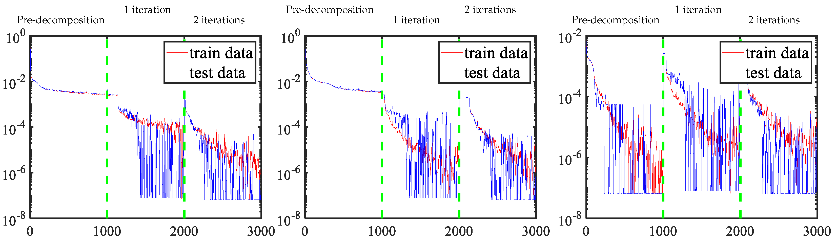
To better understand the behavior of each module in the proposed method, Figure 9 shows the loss function update curves for each material across modules. In the pre-decomposition module, the adipose and fibroglandular materials fail to achieve machine precision, but a higher proportion of calcification materials achieve machine precision. In the iterative refinement process, the accuracy is significantly improved using the residual-to-residual strategy. It is noteworthy that our framework employs a module-to-module training strategy; the initial 1000 iterations constitute the pretraining phase with exclusive loss updates, followed by two successive optimization windows (iterations 1000–2000 and 2000–3000) corresponding to first and second iterative refinement stages, respectively. Crucially, each training phase recommences with randomly initialized parameters, inherently inducing expected discontinuities in basis material decomposition across different iteration counts due to this deliberate parameter reinitialization protocol.
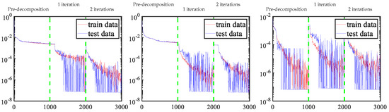
Figure 9.
Update curves of three material loss functions. Left to right: adipose, fibroglandular, and calcification material.
4.3. Residual Analysis
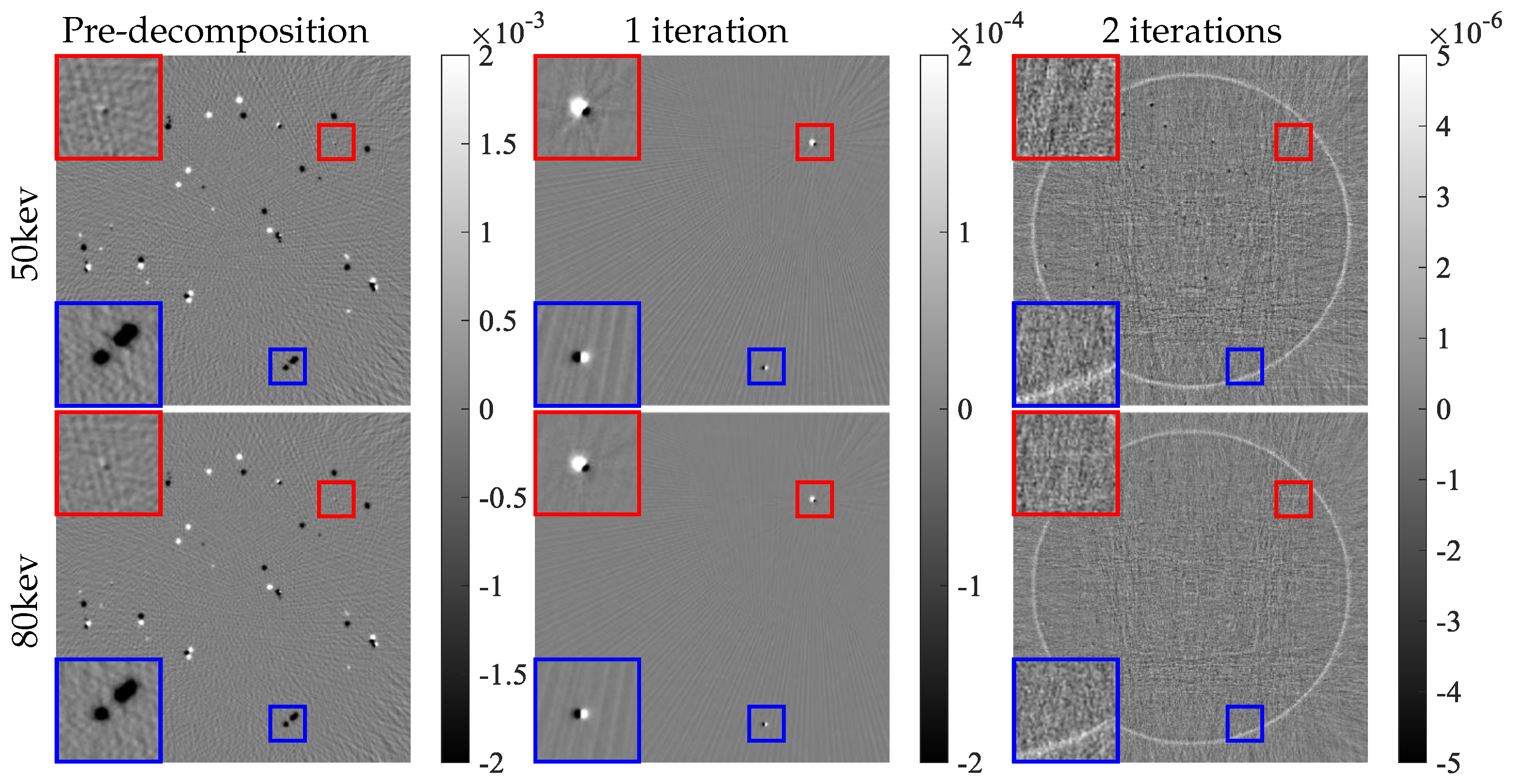
Because the projection data in the AAPM challenge are noise-free, a crucial criterion for evaluating a proper solver for this DL spectral-CT problem is minimizing the difference images , which should be as low as possible. We analyze this aspect in Figure 10. For enhanced analytical clarity, we reconstructed the residual images from the projection residuals. Figure 11 displays these reconstructed residual images. Notably, the residual images in the image domain exhibit a monotonically decreasing trend. The final iteration results demonstrate that all residual pixel values fall within machine precision.
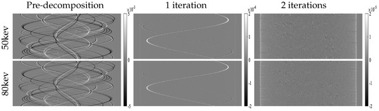
Figure 10.
Errors of projection domain for each module.
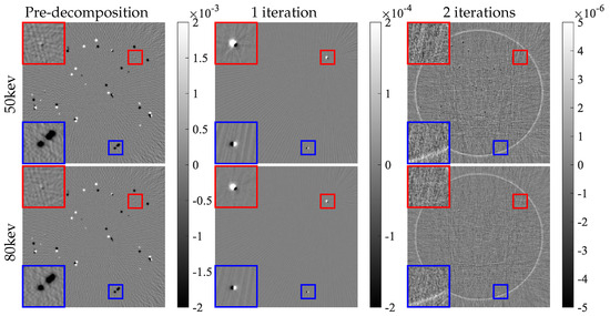
Figure 11.
Errors of image domain for each module. Colored boxes mark the trend of updates during the iterative process; corresponding zoomed-in views are displayed in the left corner.
Some pixels with small residuals (marked by red boxes in Figure 11) cannot be updated effectively in the first iteration, and are shown to be more obvious in the residual image after one iteration, which facilitates further performance improvement. Certain regions with large errors can continuously shrink during the iteration process, although the updates still have larger errors, as marked by the blue boxes.
4.4. Performance of JLRM in Noise Suppression
To ensure universality, we also studied the case of noisy data. The statistics of X-ray measurements are often described using a Poisson distribution to model the incident intensity:
where and denote the received intensity of detectors and noise-free projection data, respectively. The noisy projection data .
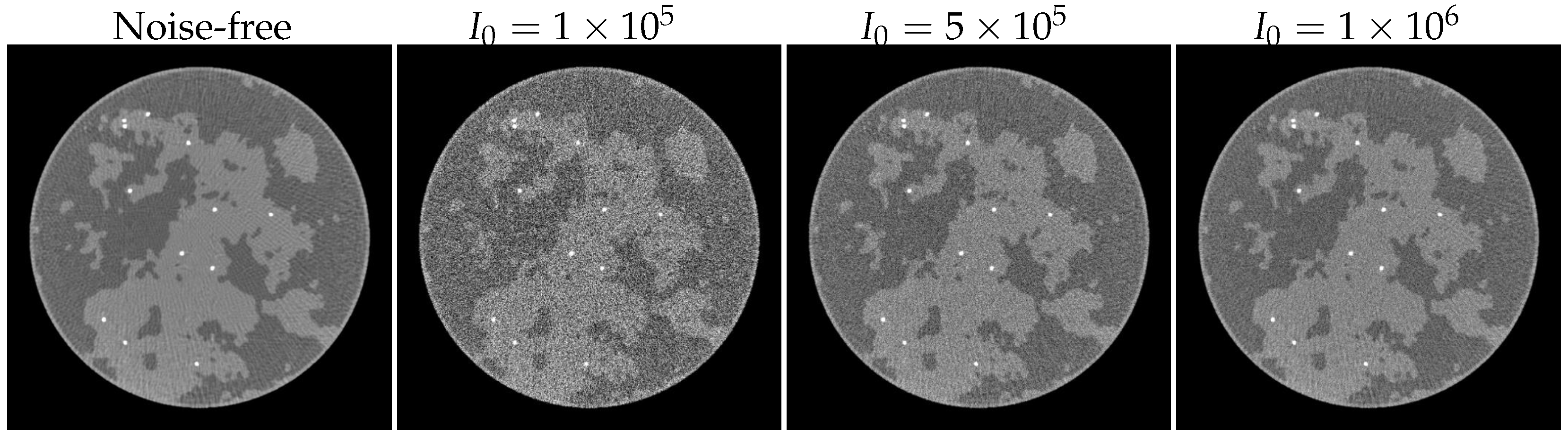
Table 3 lists the accuracy of the proposed method under different noise levels. As shown in previous experiments, the observations for adipose and fibroglandular materials are consistent, primarily because their attenuation coefficients are nearly identical. Hence, these two materials are prone to decomposition errors, and their performance metrics align closely. The calcification material, however, has a significantly higher attenuation coefficient and a much smaller spatial extent. Even under high noise levels (), calcification achieves machine precision, while under lower noise () it converges to this precision rapidly. To better demonstrate the noise characteristics, Figure 12 shows the results of FBP reconstruction applied directly to 80 kV projection data.
Table 3.
Average RMSE of dataset with different noise levels for quantitative evaluation.
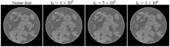
Figure 12.
FBP results with different noise levels. The display windows are .
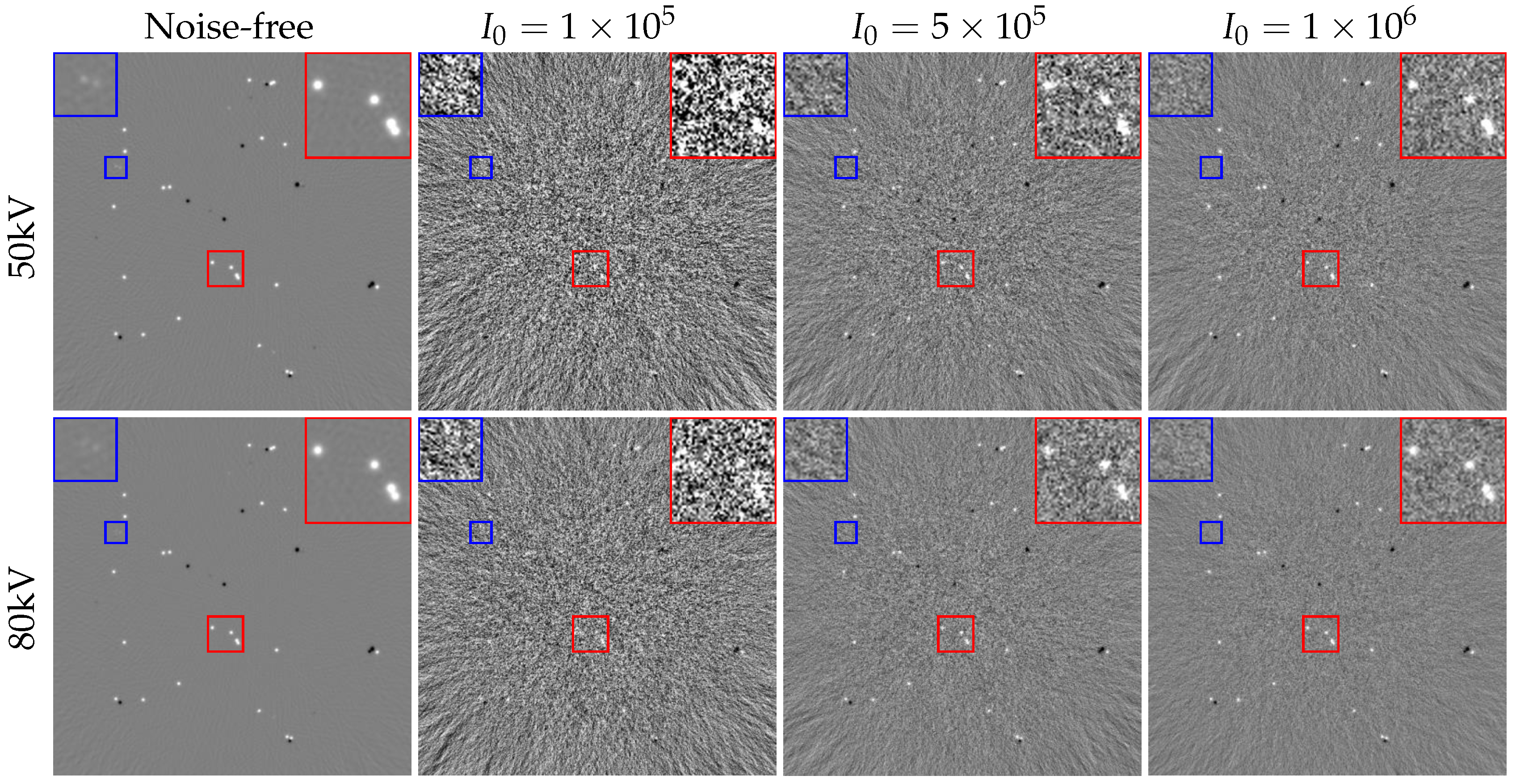
To further understand the effect of noise on the decomposition results of adipose and fibroglandular materials, we analyzed a set of results obtained from noise-free pre-decomposition. As in the residual analysis of Section 4.3, the obtained projection domain residuals are reconstructed to obtain the results shown in Figure 13, where the projection residuals are obtained by performing the physical process with the pre-decomposition results minus the noisy projections, i.e., . Figure 13 demonstrates that decomposition errors in high-noise regions (e.g., red box, zoomed view in the upper-right corner) are challenging to visualize, whereas in low-noise regions (blue box, zoomed view in the upper-left corner) errors become visually apparent only in noise-free cases. Additionally, the primary decomposition errors in noisy reconstructions are localized to edge regions.
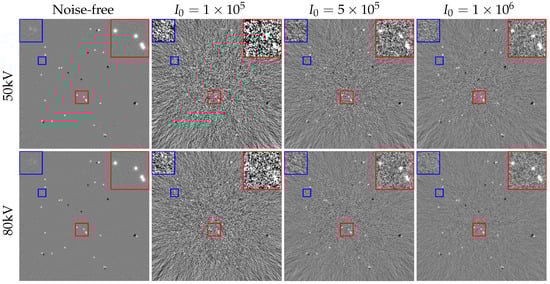
Figure 13.
Residual images with different noise levels. Colored boxes mark details of images under different noise levels, corresponding zoomed-in views are displayed in upper corners. The display windows are . Visually, with fewer photons, the amount of noise increases, leading to reduced precision in resolving fine structures during the iterative process.
4.5. Reconstruction Method: FBP vs. E-ART
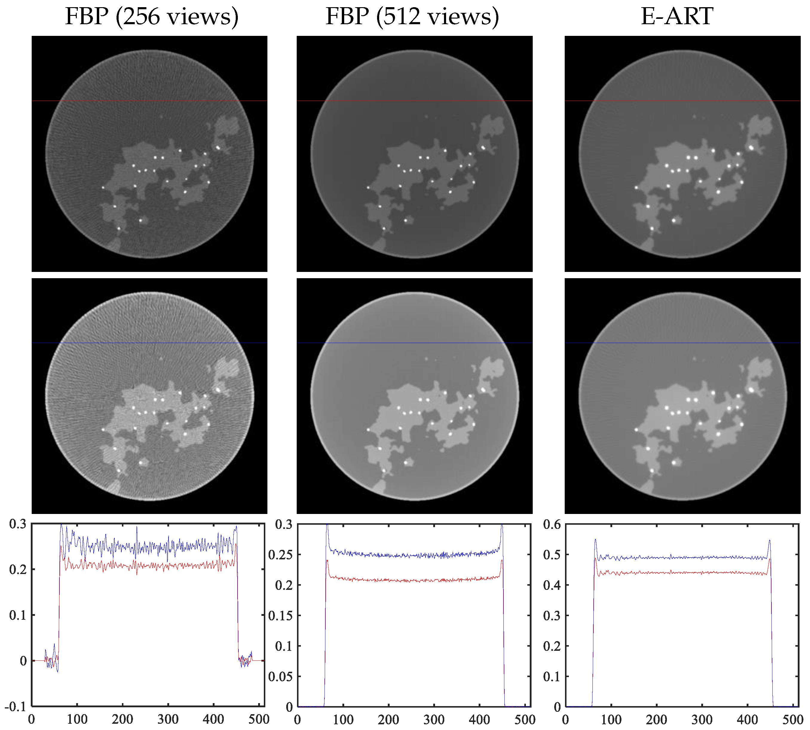
Next, we verify and analyze each part of the module mentioned in Section 3. We analyze reconstruction algorithms, including traditional analytical reconstruction (FBP) and iterative reconstruction algorithms (E-ART). For fairer comparison, we obtain higher-sampled projection data, i.e., 512 views of projection data (original 256 views), according to the projection operator provided by the official. The left two columns of Figure 14 display the reconstruction results of the FBP analytic algorithm. The right column shows the results of original projection data (256 views) using the E-ART iteration algorithm. The last row displays the profile of the mask in the first two rows.
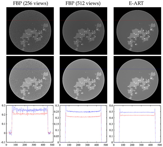
Figure 14.
Selection of reconstruction methods. First two columns: reconstruction results of FBP analytic algorithm with 256 views and 512 views. Last column: result of E-ART iteration algorithm. Last row: profile of mask in images.
There are linear artifacts caused by angle sparsity in the image reconstructed from the original data, and the reconstructed image quality is not high. Regarding the images in the middle column of the image and the cross-sectional view, it can be seem that the reconstructed image under the higher sampling projection data has a certain cup-shaped artifact. For the E-ART algorithm, although the base material images cannot be decomposed quickly in one iteration, the cup artifact is suppressed well and the linear artifact caused by sparse sampling can be effectively alleviated by setting the relaxation factor appropriately, which benefits subsequent network decomposition. It should be noted here that FBP ignores the energy spectrum and directly reconstructs the grayscale value. The grayscale value of the base material decomposition using E-ART is different, but can be used to analyze the advantages of E-ART over FBP and to facilitate subsequent decomposition.
4.6. Receptive Field: Small or Large
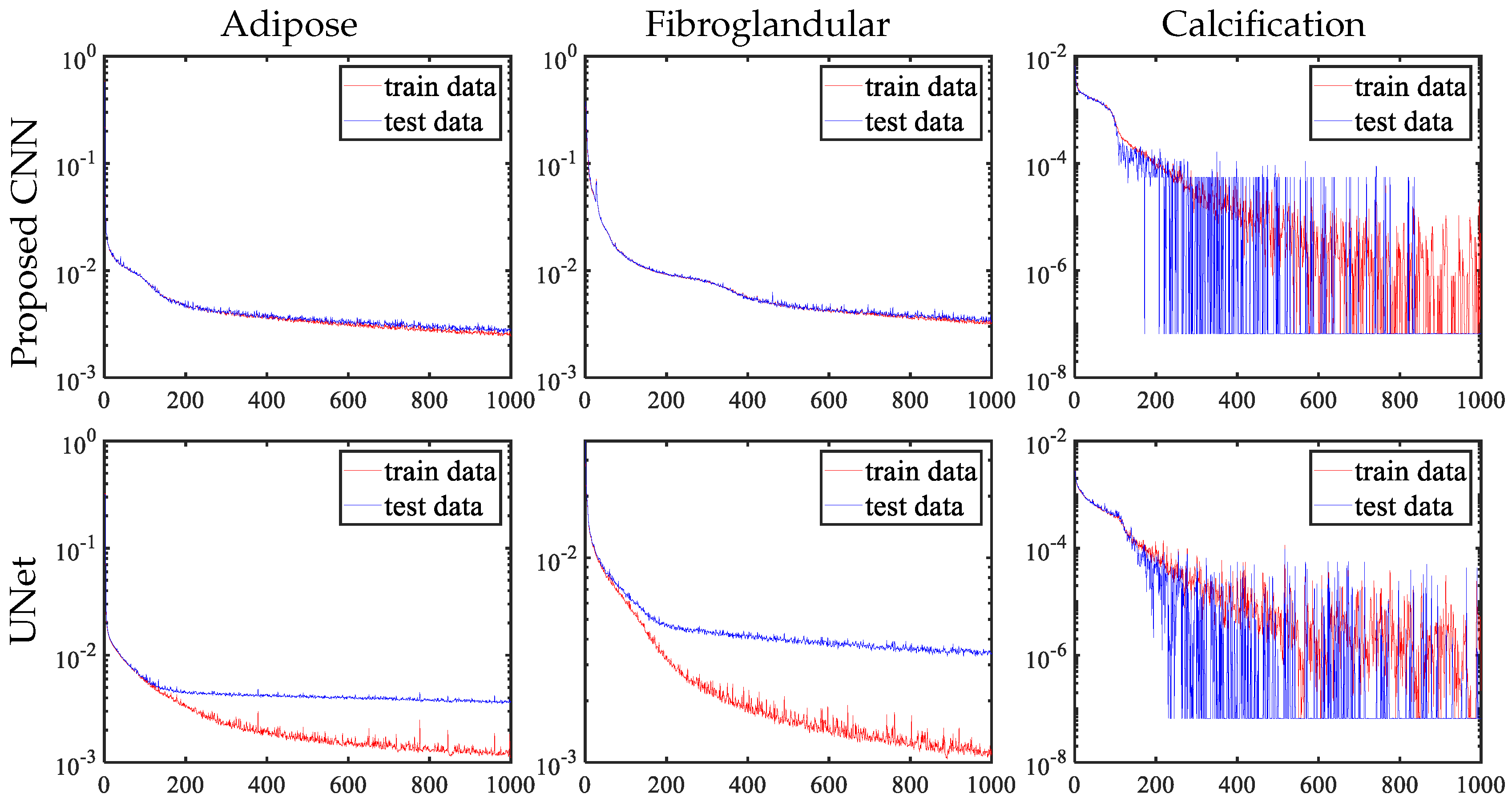
As argued in the CNN network structure design of Section 3, increasing the receptive field will aggravate the overfitting phenomenon, which is fatal to the goal of obtaining more accurate decomposition results in later iterations. Figure 15 shows the loss function curve update of the pre-decomposition module. During the training process of the proposed CNN, the changes of the training and test sets are essentially the same with the iterative update. For UNet, using pooling and upsampling layers causes the network to have a large receptive field, where other network parameters (such as the number of layers, channels and kernel size of convolution) are same as the proposed CNN. However, the experimental results show that adipose and fibroglandular materials display an obvious overfitting phenomenon after a period of training.

Figure 15.
Update curves of three material loss functions for pre-decomposition module with networks having different receptive fields.
Figure 16 shows the performance of overfitting in the reconstructed image of adipose material, where fibroglandular material has the same phenomenon. The training set has higher accuracy for UNet, and the error in the difference image is quite small, while the test set has a significantly larger error. Table 4 also displays the RMSE performance metrics of the two network designs. In comparing the training and test set results, severe overfitting can be observed with the UNet architecture, while the proposed CNN model effectively mitigates this issue. This contrast not only highlights the robustness of our CNN design but also validates the effectiveness of the iterative training strategy in maintaining generalization capability.
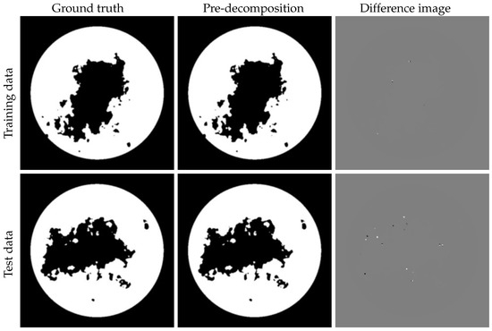
Figure 16.
Results of reconstruction of training and test data using a larger receptive field. Display windows: [0,1] for material images, and [−0.05,0.05] for difference images.
Table 4.
Average RMSE of dataset with different network structure for quantitative evaluation.
4.7. Residual-to-Residual vs. Image-to-Residual
Next, we investigate the mapping strategy. Figure 17 displays partial results of two iterations for adipose and fibroglandular materials using the image-to-residual and residual-to-residual mapping strategies. The image-to-residual strategy introduces new reconstruction errors, leading to limited accuracy improvement and potential instability, as regions with large errors are visually indistinguishable in reconstructed images. In contrast, the residual-to-residual strategy achieves significantly higher accuracy. This improvement stems from two factors: (1) integration with the physical module to calculate residuals, and (2) avoidance of floating-point precision loss thanks to the residual-to-residual training strategy.
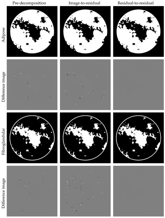
Figure 17.
Results for the residual-to-residual and image-to-residual mapping strategies. Display windows: [0,1] for material images and [−0.05,0.05] for different images. It can be clearly seen that the image-to-residual strategy iterations would be rendered meaningless by the introduction of new errors. On the other hand, the proposed residual-to-residual approach achieves a rational improvement.
5. Summary
To solve the problem of high-precision base material decomposition in spectral CT, this paper proposes an algorithm fusing a physical model, model-based iterative reconstruction, and deep learning. Each part has clear functions and is constructed based on given problems and actual situations. The physical module, which is embedded and expressed as a network structure, can accurately describe the physical process of SCT imaging, while the model-based iterative reconstruction algorithm realizes information transfer between domains. Together, the three modules complement each other. We introduce some network skills or strategies in the proposed modules, which are based on observations related to SCT problems and can improve the reconstruction results. The key methodological innovations include:
- Synergistic integration of complementary components: By integrating physical processing (for nonlinear SCT physics), MBIR (for stable domain transformations), and deep learning (for material decomposition), the proposed method combines the interpretability of physics-driven models with the adaptability of neural networks. The physical component ensures fidelity to fundamental X-ray interactions, MBIR provides robustness against noise and incomplete data, and the neural network resolves ambiguities in material-specific attenuation profiles.
- Network-embedded physical model: A network-integrated physical model governs SCT projection data generation, enabling more accurate representation of SCT physical processes. The iterative process progressively enhances reconstruction accuracy through comprehensive physical modeling, where the SCT physical framework is implemented as a network module with learnable parameters including X-ray spectra and attenuation coefficients .
- Residual-to-residual training: The training paradigm employs residual-to-residual mapping rather than conventional image-to-image or image-to-residual approaches. This strategy focuses on error-sensitive regions that are visually identifiable in residual images but indistinguishable in original reconstructions. This is a novel training paradigm that prioritizes error-sensitive regions by mapping residual projections to residual images.
- Network structure design: The network architecture addresses practical constraints through domain-specific design by (1) accounting for limited spatial correlations between SCT projection data and reconstructed images under inconsistent projections and (2) optimizing CNN receptive field size to balance feature extraction capability with prevention of overfitting and robustness degradation.
6. Limitations
While the proposed method demonstrates significant advancements in spectral CT (SCT) reconstruction, two critical limitations hinder its broader applicability and performance optimization:
- Modular disconnection in network training: The current framework adopts a modular reassembly strategy in which the physical model, MBIR, and deep learning components are trained in a distributed manner. Although this design simplifies implementation (e.g., pretraining the physics module independently), it restricts synergistic interactions between modules. For example, updates to the physical parameters (e.g., X-ray spectra ) are based on localized loss functions rather than global feedback from the downstream decomposition task. This fragmented optimization prevents end-to-end error propagation, potentially underutilizing the physical model’s capacity to guide holistic reconstruction. A fully-integrated organic training framework in which modules co-evolve through shared gradients could better harmonize physics constraints with data-driven priors, likely improving reconstruction accuracy.
- Narrow data scope and limited spectral diversity: Validation relied primarily on the AAPM Challenge dataset, which uses synthetic projections generated from a single known X-ray spectrum. While effective for proof-of-concept, this setup overlooks real-world complexities such as spectral drift, detector nonlinearity, and patient-specific anatomical variations. Material decomposition accuracy may degrade when applied to clinical data with unknown or mixed spectra (e.g., dual-energy CT with vendor-specific beam hardening corrections), highlighting the need for validation across diverse scanner configurations and patient populations.
To address these limitations, future work should prioritize two key directions while preserving the method’s core innovations, specifically, unified training paradigms and data-driven generalization. (1) End-to-End Physics–Network Co-Training: Replacing the current module-to-module training strategy with a unified framework where physical parameters () and network weights are jointly optimized through a shared loss function would enable the physical model to dynamically adapt to material decomposition feedback, closing the loop between projection generation and image reconstruction; for instance, spectral corrections could directly respond to errors, fostering tighter integration between physics and learning. (2) Multi-Source Data Augmentation and Spectral Transfer Learning: Training should be expanded to diverse clinical datasets with heterogeneous spectra (e.g., photon-counting CT, dual-source CT) and real-world artifacts (e.g., scatter, motion). A spectral domain adaptation module could be introduced to align simulated and clinical data distributions, while few-shot learning techniques might mitigate data scarcity for rare materials or pathologies.
Despite its limitations, the proposed method effectively bridges physics-based modeling and deep learning for spectral CT reconstruction, achieving state-of-the-art material decomposition accuracy on standardized benchmarks. While suboptimal in training cohesion, the modular design successfully demonstrates the value of embedding interpretable physical parameters () within a learning framework. However, the reliance on synthetic data and fragmented optimization underscores a gap between theoretical innovation and clinical readiness.
Future efforts to unify training workflows and expand data diversity will be pivotal in translating this method into a robust clinical tool. By addressing these challenges, the proposed approach holds promise for advancing spectral imaging toward personalized diagnostics in which physics-guided AI synergizes with real-world clinical complexity to deliver precise and actionable insights.
Author Contributions
Conceptualization, G.M.; methodology, G.M. and X.Z.; software, G.M.; validation, G.M.; formal analysis, G.M. and P.Y.; investigation, G.M.; resources, G.M.; data curation: G.M.; writing—original draft preparation, G.M. and P.Y.; writing—review and editing, G.M., P.Y. and X.Z.; visualization, G.M. and P.Y.; supervision, X.Z.; funding acquisition, G.M. and X.Z. All authors have read and agreed to the published version of the manuscript.
Funding
This research is supported by National Natural Science Foundation of China, Grant/Award Numbers (12426308) and the National Key Research and Development Program of China, Grant/Award Number (2023YFA1011402), Beijing Postdoctoral Research Foundation and the Key Research Project of the Academy for Multidisciplinary Studies, Capital Normal University. The authors are also grateful to National Center for Applied Mathematics Beijing for funding this research work.
Data Availability Statement
The datasets used in the paper have been sourced in the article. The author has no right to share the datasets. The corresponding official datasets for the experiments can be found according to the provided links.
Conflicts of Interest
Author Genwei Ma is an employee of National Center for Applied Mathematics Beijing, Capital Normal University. The remaining authors declare that the research was conducted in the absence of any commercial or financial relationships that could be construed as a potential conflict of interest.
References
- Xu, D.; Langan, D.A.; Wu, X.; Pack, J.D.; Benson, T.M.; Tkaczky, J.E.; Schmitz, A.M. Dual energy CT via fast kVp switching spectrum estimation. In Medical Imaging 2009: Physics of Medical Imaging; SPIE: Bellingham, WA, USA, 2009; Volume 7258, pp. 1198–1207. [Google Scholar]
- Petersilka, M.; Bruder, H.; Krauss, B.; Stierstorfer, K.; Flohr, T.G. Technical principles of dual source CT. Eur. J. Radiol. 2008, 68, 362–368. [Google Scholar] [CrossRef] [PubMed]
- Willemink, M.J.; Persson, M.; Pourmorteza, A.; Pelc, N.J.; Fleischmann, D. Photon-counting CT: Technical Principles and Clinical Prospects. Radiology 2018, 289, 293–312. [Google Scholar] [CrossRef]
- Leng, S.; Bruesewitz, M.; Tao, S.; Rajendran, K.; Halaweish, A.F.; Campeau, N.G.; Fletcher, J.G.; McCollough, C.H. Photon-counting Detector CT: System Design and Clinical Applications of an Emerging Technology. Radiographics 2019, 39, 729–743. [Google Scholar] [CrossRef] [PubMed]
- Alvarez, R.E.; Macovski, A. Energy-selective reconstructions in X-ray computerised tomography. Phys. Med. Biol. 1976, 21, 733. [Google Scholar] [CrossRef]
- Alvarez, R.; Seppi, E. A comparison of noise and dose in conventional and energy selective computed tomography. IEEE Trans. Nucl. Sci. 1979, 26, 2853–2856. [Google Scholar] [CrossRef]
- Alvarez, R.E.; Seibert, J.A.; Thompson, S.K. Comparison of dual energy detector system performance. Med. Phys. 2004, 31, 556–565. [Google Scholar] [CrossRef]
- Kalender, W.A.; Perman, W.; Vetter, J.; Klotz, E. Evaluation of a prototype dual-energy computed tomographic apparatus. I. Phantom studies. Med. Phys. 1986, 13, 334–339. [Google Scholar] [CrossRef]
- Yu, L.; Leng, S.; McCollough, C.H. Dual-energy CT–based monochromatic imaging. Am. J. Roentgenol. 2012, 199, S9–S15. [Google Scholar] [CrossRef]
- Brooks, R.A.; Di Chiro, G. Beam hardening in X-ray reconstructive tomography. Phys. Med. Biol. 1976, 21, 390. [Google Scholar] [CrossRef] [PubMed]
- Coleman, A.; Sinclair, M. A beam-hardening correction using dual-energy computed tomography. Phys. Med. Biol. 1985, 30, 1251. [Google Scholar] [CrossRef]
- Cardinal, H.N.; Fenster, A. An accurate method for direct dual-energy calibration and decomposition. Med. Phys. 1990, 17, 327–341. [Google Scholar] [CrossRef]
- Dong, X.; Niu, T.; Zhu, L. Combined iterative reconstruction and image-domain decomposition for dual energy CT using total-variation regularization. Med. Phys. 2014, 41, 051909. [Google Scholar] [CrossRef]
- Zeng, D.; Huang, J.; Zhang, H.; Bian, Z.; Niu, S.; Zhang, Z.; Feng, Q.; Chen, W.; Ma, J. Spectral CT image restoration via an average image-induced nonlocal means filter. IEEE Trans. Biomed. Eng. 2015, 63, 1044–1057. [Google Scholar] [CrossRef] [PubMed]
- Stenner, P.; Berkus, T.; Kachelriess, M. Empirical dual energy calibration (EDEC) for cone-beam computed tomography. Med. Phys. 2007, 34, 3630–3641. [Google Scholar] [CrossRef] [PubMed]
- Maaß, N.; Sawall, S.; Knaup, M.; Kachelrieß, M. Empirical multiple energy calibration (EMEC) for material-selective CT. In Proceedings of the 2011 IEEE Nuclear Science Symposium Conference Record, Valencia, Spain, 23–29 October 2011; pp. 4222–4229. [Google Scholar]
- Ying, Z.; Naidu, R.; Crawford, C.R. Dual energy computed tomography for explosive detection. J. X-ray Sci. Technol. 2006, 14, 235–256. [Google Scholar] [CrossRef]
- Maaß, C.; Meyer, E.; Kachelrieß, M. Exact dual energy material decomposition from inconsistent rays (MDIR). Med. Phys. 2011, 38, 691–700. [Google Scholar] [CrossRef]
- Feng, C.; Shen, Q.; Kang, K.; Xing, Y. An empirical material decomposition method (EMDM) for spectral CT. In Proceedings of the 2016 IEEE Nuclear Science Symposium, Medical Imaging Conference and Room-Temperature Semiconductor Detector Workshop (NSS/MIC/RTSD), Strasbourg, France, 29 October–6 November 2016; pp. 1–5. [Google Scholar]
- Sukovic, P.; Clinthorne, N.H. Penalized weighted least-squares image reconstruction for dual energy X-ray transmission tomography. IEEE Trans. Med. Imaging 2000, 19, 1075–1081. [Google Scholar] [CrossRef]
- Elbakri, I.A.; Fessler, J.A. Statistical image reconstruction for polyenergetic X-ray computed tomography. IEEE Trans. Med. Imaging 2002, 21, 89–99. [Google Scholar] [CrossRef]
- Xu, Q.; Mou, X.; Tang, S.; Hong, W.; Zhang, Y.; Luo, T. Implementation of penalized-likelihood statistical reconstruction for polychromatic dual-energy CT. In Medical Imaging 2009: Physics of Medical Imaging; SPIE: Bellingham, WA, USA, 2009; Volume 7258, pp. 1666–1674. [Google Scholar]
- Long, Y.; Fessler, J.A. Multi-material decomposition using statistical image reconstruction for spectral CT. IEEE Trans. Med. Imaging 2014, 33, 1614–1626. [Google Scholar] [CrossRef]
- Niu, T.; Dong, X.; Petrongolo, M.; Zhu, L. Iterative image-domain decomposition for dual-energy CT. Med. Phys. 2014, 41, 041901. [Google Scholar] [CrossRef]
- Zhang, R.; Thibault, J.B.; Bouman, C.A.; Sauer, K.D.; Hsieh, J. Model-based iterative reconstruction for dual-energy X-ray CT using a joint quadratic likelihood model. IEEE Trans. Med. Imaging 2013, 33, 117–134. [Google Scholar] [CrossRef] [PubMed]
- Zhao, Y.; Zhao, X.; Zhang, P. An extended algebraic reconstruction technique (E-ART) for dual spectral CT. IEEE Trans. Med. Imaging 2014, 34, 761–768. [Google Scholar] [CrossRef] [PubMed]
- Hu, J.; Zhao, X.; Wang, F. An extended simultaneous algebraic reconstruction technique (E-SART) for X-ray dual spectral computed tomography. Scanning 2016, 38, 599–611. [Google Scholar] [CrossRef] [PubMed]
- Chen, B.; Zhang, Z.; Sidky, E.Y.; Xia, D.; Pan, X. Image reconstruction and scan configurations enabled by optimization-based algorithms in multispectral CT. Phys. Med. Biol. 2017, 62, 8763. [Google Scholar] [CrossRef]
- Li, M.; Zhao, Y.; Zhang, P. Accurate iterative FBP reconstruction method for material decomposition of dual energy CT. IEEE Trans. Med. Imaging 2018, 38, 802–812. [Google Scholar] [CrossRef]
- Zhao, S.; Pan, H.; Zhang, W.; Xia, D.; Zhao, X. An oblique projection modification technique (OPMT) for fast multispectral CT reconstruction. Phys. Med. Biol. 2021, 66, 065003. [Google Scholar] [CrossRef]
- Zhang, W.; Zhao, S.; Pan, H.; Zhao, Y.; Zhao, X. An iterative reconstruction method based on monochromatic images for dual energy CT. Med. Phys. 2021, 48, 6437–6452. [Google Scholar] [CrossRef]
- Sawatzky, A.; Xu, Q.; Schirra, C.O.; Anastasio, M.A. Proximal ADMM for multi-channel image reconstruction in spectral X-ray CT. IEEE Trans. Med. Imaging 2014, 33, 1657–1668. [Google Scholar] [CrossRef]
- Barber, R.F.; Sidky, E.Y.; Schmidt, T.G.; Pan, X. An algorithm for constrained one-step inversion of spectral CT data. Phys. Med. Biol. 2016, 61, 3784. [Google Scholar] [CrossRef]
- Touch, M.; Clark, D.P.; Barber, W.; Badea, C.T. A neural network-based method for spectral distortion correction in photon counting X-ray CT. Phys. Med. Biol. 2016, 61, 6132. [Google Scholar] [CrossRef]
- Liao, Y.; Wang, Y.; Li, S.; He, J.; Zeng, D.; Bian, Z.; Ma, J. Pseudo dual energy CT imaging using deep learning-based framework: Basic material estimation. In Medical Imaging 2018: Physics of Medical Imaging; SPIE: Bellingham, WA, USA, 2018; Volume 10573, pp. 1190–1194. [Google Scholar]
- Zhao, W.; Vernekohl, D.; Han, F.; Han, B.; Peng, H.; Yang, Y.; Xing, L.; Min, J.K. A unified material decomposition framework for quantitative dual-and triple-energy CT imaging. Med. Phys. 2018, 45, 2964–2977. [Google Scholar] [CrossRef]
- Xu, Y.; Yan, B.; Chen, J.; Zeng, L.; Li, L. Projection decomposition algorithm for dual-energy computed tomography via deep neural network. J. X-ray Sci. Technol. 2018, 26, 361–377. [Google Scholar] [CrossRef]
- Xu, Y.; Yan, B.; Zhang, J.; Chen, J.; Zeng, L.; Wang, L. Image decomposition algorithm for dual-energy computed tomography via fully convolutional network. Comput. Math. Methods Med. 2018, 2018, 2527516. [Google Scholar] [CrossRef] [PubMed]
- Hu, D.; Wu, W.; Xu, M.; Zhang, Y.; Liu, J.; Ge, R.; Chen, Y.; Luo, L.; Coatrieux, G. SISTER: Spectral-image similarity-based tensor with enhanced-sparsity reconstruction for sparse-view multi-energy CT. IEEE Trans. Comput. Imaging 2019, 6, 477–490. [Google Scholar] [CrossRef]
- Wu, X.; He, P.; Long, Z.; Guo, X.; Chen, M.; Ren, X.; Chen, P.; Deng, L.; An, K.; Li, P.; et al. Multi-material decomposition of spectral CT images via Fully Convolutional DenseNets. J. X-ray Sci. Technol. 2019, 27, 461–471. [Google Scholar] [CrossRef] [PubMed]
- Li, D.; Li, S.; Zhu, M.; Gao, Q.; Bian, Z.; Huang, H.; Zhang, S.; Huang, J.; Zeng, D.; Ma, J. Unsupervised data fidelity enhancement network for spectral CT reconstruction. In Medical Imaging 2020: Physics of Medical Imaging; SPIE: Bellingham, WA, USA, 2020; Volume 11312, pp. 1081–1088. [Google Scholar]
- Yao, L.; Li, S.; Li, D.; Zhu, M.; Gao, Q.; Zhang, S.; Bian, Z.; Huang, J.; Zeng, D.; Ma, J. Leveraging deep generative model for direct energy-resolving CT imaging via existing energy-integrating CT images. In Medical Imaging 2020: Physics of Medical Imaging; SPIE: Bellingham, WA, USA, 2020; Volume 11312, pp. 1190–1195. [Google Scholar]
- Primak, A.; Ramirez Giraldo, J.; Liu, X.; Yu, L.; McCollough, C.H. Improved dual-energy material discrimination for dual-source CT by means of additional spectral filtration. Med. Phys. 2009, 36, 1359–1369. [Google Scholar] [CrossRef] [PubMed]
- Flohr, T.G.; McCollough, C.H.; Bruder, H.; Petersilka, M.; Gruber, K.; Süβ, C.; Grasruck, M.; Stierstorfer, K.; Krauss, B.; Raupach, R.; et al. First performance evaluation of a dual-source CT (DSCT) system. Eur. Radiol. 2006, 16, 256–268. [Google Scholar] [CrossRef]
- Shan, H.; Padole, A.; Homayounieh, F.; Kruger, U.; Khera, R.D.; Nitiwarangkul, C.; Kalra, M.K.; Wang, G. Competitive performance of a modularized deep neural network compared to commercial algorithms for low-dose CT image reconstruction. Nat. Mach. Intell. 2019, 1, 269–276. [Google Scholar] [CrossRef]
- Sidky, E.Y.; Pan, X. Report on the AAPM deep-learning spectral CT Grand Challenge. Med. Phys. 2024, 51, 772–785. [Google Scholar] [CrossRef]
- Genzel, M.; Gühring, I.; Macdonald, J.; März, M. Near-Exact Recovery for Tomographic Inverse Problems via Deep Learning. In Proceedings of the 39th International Conference on Machine Learning, PMLR, Baltimore, MD, USA, 17–23 July 2022; pp. 7368–7381. [Google Scholar]
- Wu, D.; Kim, K.; Li, Q. Computationally efficient deep neural network for computed tomography image reconstruction. Med. Phys. 2019, 46, 4763–4776. [Google Scholar] [CrossRef]
- Adler, J.; Öktem, O. Learned primal-dual reconstruction. IEEE Trans. Med. Imaging 2018, 37, 1322–1332. [Google Scholar] [CrossRef]
- Dhar, P.; Singh, R.V.; Peng, K.C.; Wu, Z.; Chellappa, R. Learning without memorizing. In Proceedings of the IEEE/CVF Conference on Computer Vision and Pattern Recognition, Long Beach, CA, USA, 15–20 June 2019; pp. 5138–5146. [Google Scholar]
- Li, Z.; Hoiem, D. Learning without forgetting. IEEE Trans. Pattern Anal. Mach. Intell. 2017, 40, 2935–2947. [Google Scholar] [CrossRef]
- Würfl, T.; Hoffmann, M.; Christlein, V.; Breininger, K.; Huang, Y.; Unberath, M.; Maier, A.K. Deep learning computed tomography: Learning projection-domain weights from image domain in limited angle problems. IEEE Trans. Med. Imaging 2018, 37, 1454–1463. [Google Scholar] [CrossRef]
- Syben, C.; Michen, M.; Stimpel, B.; Seitz, S.; Ploner, S.; Maier, A.K. PYRO-NN: Python reconstruction operators in neural networks. Med. Phys. 2019, 46, 5110–5115. [Google Scholar] [CrossRef]
- Reiser, I.; Nishikawa, R. Task-based assessment of breast tomosynthesis: Effect of acquisition parameters and quantum noise a. Med. Phys. 2010, 37, 1591–1600. [Google Scholar] [CrossRef]


Disclaimer/Publisher’s Note: The statements, opinions and data contained in all publications are solely those of the individual author(s) and contributor(s) and not of MDPI and/or the editor(s). MDPI and/or the editor(s) disclaim responsibility for any injury to people or property resulting from any ideas, methods, instructions or products referred to in the content. |
© 2025 by the authors. Licensee MDPI, Basel, Switzerland. This article is an open access article distributed under the terms and conditions of the Creative Commons Attribution (CC BY) license (https://creativecommons.org/licenses/by/4.0/).