Fluid and Dynamic Analysis of Space–Time Symmetry in the Galloping Phenomenon

Abstract

Energy generation from renewable sources has increased exponentially worldwide, particularly wind energy, which is converted into electricity through wind turbines. The growing demand for renewable energy has driven the development of horizontal-axis wind turbines with larger dimensions, as the energy captured is proportional to the area swept by the rotor blades. In this context, the dynamic loads typically observed in wind turbine towers include vibrations caused by rotating blades at the top of the tower, wind pressure, and earthquakes (less common). In offshore wind farms, wind turbine towers are also subjected to dynamic loads from waves and ocean currents. Vortex-induced vibration can be an undesirable phenomenon, as it may lead to significant adverse effects on wind turbine structures. This study presents a two-dimensional transient model for a rigid body anchored by a torsional spring subjected to a constant velocity flow. We applied a coupling of the Fourier pseudospectral method (FPM) and immersed boundary method (IBM), referred to in this study as IMERSPEC, for a two-dimensional, incompressible, and isothermal flow with constant properties—the FPM to solve the Navier–Stokes equations, and IBM to represent the geometries. Computational simulations, solved at an aspect ratio of $\varphi =4.0$, were analyzed, considering Reynolds numbers ranging from $Re=150$ to Re = 1000 when the cylinder is stationary, and $Re=250$ when the cylinder is in motion. In addition to evaluating vortex shedding and Strouhal number, the study focuses on the characterization of space–time symmetry during the galloping response. The results show a spatial symmetry breaking in the flow patterns, while the oscillatory motion of the rigid body preserves temporal symmetry. The numerical accuracy suggested that the IMERSPEC methodology can effectively solve complex problems. Moreover, the proposed IMERSPEC approach demonstrates notable advantages over conventional techniques, particularly in terms of spectral accuracy, low numerical diffusion, and ease of implementation for moving boundaries. These features make the model especially efficient and suitable for capturing intricate fluid–structure interactions, offering a promising tool for analyzing wind turbine dynamics and other similar systems.

1. Introduction

Computational fluid dynamics (CFD) has been widely used in several applications over the past decade, contributing significantly to the technological development in the aeronautics, oil, automotive, and energy sectors. Increasingly accurate models have been applied to identify hydrodynamic coefficients and understand the physical phenomenon by representing the turbulent structures of the flow over immersed bodies. In addition, immersed bodies may also move as a result of the flow, characterizing a fluid–structure interaction (FSI) problem. Thus, the motion of the fluid and the immersed body should be determined using transient models.

For these applications, we can use discretization methods, such as the finite volume method (FVM) or Fourier pseudospectral method (FPM), to simulate the fluid and other forms. Nascimento et al. [1] reported that FPM reduced computational cost compared to FVM since it did not require solving the linear system of the pressure–velocity coupling, maintaining the accuracy and convergence order of the solutions.

In computational implementation, accurately identifying structures of complex, movable, or deformable geometries over time inside the flow can be a challenge when simulating FSI problems. Two approaches are commonly used to simulate immersed bodies: body-fitted meshes and non-body-fitted meshes. The second one is used in the immersed boundary method (IBM). IBM has emerged as an efficient alternative to body-fitted meshes for handling FSI problems. In IBM, the immersed body is represented by a forcefield inserted into the fluid equations. This indirectly models the immersed body. Peskin [2] developed this method to simulate blood flow in heart valves.

For modeling the structure behavior in FSI problems, we can consider a rigid structure or a deformable solid. The first option is applicable when small deformations are anticipated, which do not significantly impact the overall behavior of the structure, allowing the floating body to be modeled as a rigid body. This assumption holds when the structural deformations are sufficiently small and do not noticeably affect the global response of the system. According to Newman [3], a floating body can be considered rigid when its internal deformation is negligible relative to the acting forces. This approach is particularly suitable for structures made of high-stiffness materials, such as steel and concrete, subjected to low-frequency excitations [4]. Additionally, Chakrabarti [5] observed that the assumption of structural rigidity remains valid when the ratio between the material stiffness and the hydrodynamic forces is high, as is often observed in metallic vessels and large-scale ocean structures. The structure behavior is modeled based on rigid body dynamics equations from the Newton–Euler equations, which allows us to determine a set of coordinates to characterize the center of mass motion and angular motion of the structure Meriam and Kraige [6]. In the second case, the structure behavior is modeled using principles from solid mechanics. In this approach, the structure is represented by a set of coordinates to identify the spatial position of each point of the structure. This approach also considers the specific mechanical properties of the material used in the structure.

Thus, the present study aimed to develop, implement, and validate a numerical methodology to represent the galloping phenomenon in fluid–structure interaction (FSI) problems. The main contributions of this work are: (1) the proposal of a novel numerical approach, IMERSPEC, based on the coupling of the Fourier pseudospectral method (FPM) and the immersed boundary method (IBM), suitable for problems with moving boundaries; (2) the implementation of an efficient strategy for data exchange between fluid and solid domains; and (3) the characterization of the galloping phenomenon response, including the identification of spatial symmetry breaking in the flow and preservation of temporal symmetry in the rigid body motion. The results obtained are validated against existing literature and demonstrate the accuracy and potential of the proposed approach for analyzing complex FSI phenomena, particularly relevant to wind turbine dynamics.

2. Relate Works

Recent studies, such as that of Zhang et al. [7], have contributed to the modeling of complex fluid behaviors, particularly the nonlinear hysteresis phenomenon in composite magnetorheological fluids. They proposed a parametric model to predict this phenomenon, providing insights into the nonlinear dynamics of these fluids, which are critical in fluid–structure interaction systems. This study is relevant for improving the design of systems that utilize magnetorheological materials, such as in vibration damping and actuation systems.

Building on foundational mathematical formulations for FSI problems, Li et al. [8] developed a high-order spectral method to model rigid body interactions with fluid flow. Their approach was validated through simulations of flow around circular cylinders at Reynolds numbers ranging from 100 to 400, capturing both free and forced motions. Further application of this method to a rectangular body at $Re=250$ revealed torsional galloping phenomena, which are a type of aeroelastic instability characterized by sustained oscillations due to fluid flow.

Expanding on this, Robertson et al. [9] investigated vibrations induced by rotational and translational galloping in rectangular cylinders with varying aspect ratios ($\varphi$ from 1 to 5) at $Re=250$. Their results qualitatively agreed with quasi-static theories and experimental data, advancing the understanding of how geometry influences FSI-induced instabilities in low-Reynolds-number flows.

The central finite difference method coupled with the direct-forcing immersed boundary methodology was applied by Yang and Stern [10] to study vortex-induced vibrations of circular cylinders, as well as transverse and rotational galloping of rectangular bodies and flutter phenomena in plates. This work demonstrated the capability of their numerical approach to accurately capture fluid-induced instabilities, corroborating previous numerical and experimental findings.

In the context of turbulence and wake dynamics, Yang and Stern [11] analyzed flow over single and arrays of aligned wind turbines using a second-order central finite difference method with unstructured meshes. They showed that turbulence generated in turbine wakes can persist over several rotor diameters downstream, an important consideration for wind farm design and optimization.

In the present study, the flow over a rectangular cylinder are investigated, a classical problem extensively examined by Li et al. [8], Robertson et al. [9], Yang and Stern [10], Nomura [12], Cui et al. [13], Siriyothai and Kittichaikarn [14], and Hémon et al. [15]. These works have characterized wake vortices and the galloping phenomenon—a self-sustained aeroelastic oscillation induced by fluid flow.

3. Materials and Methods

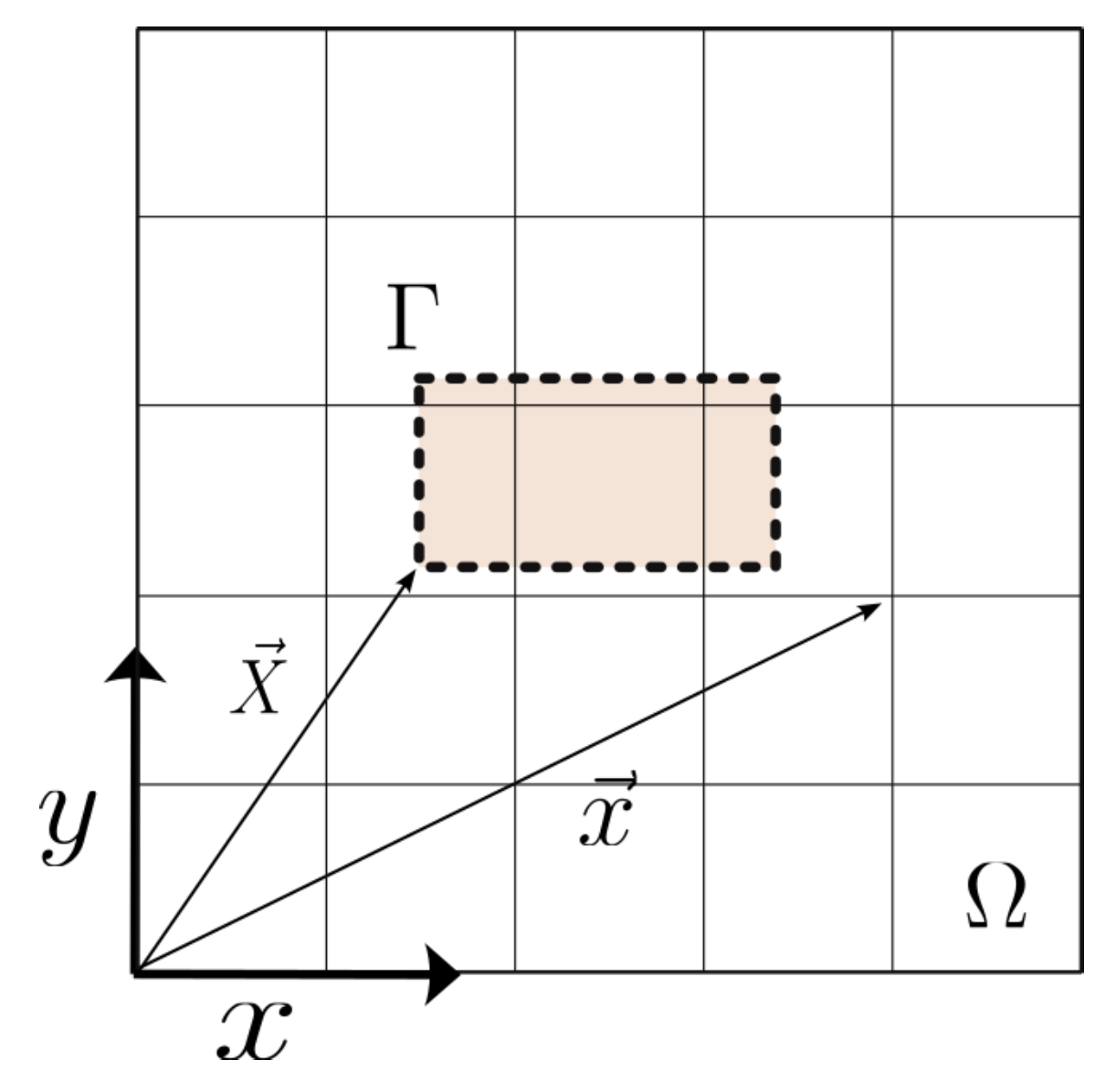
3.1. Mathematical Model

The coupling of flow and structural models was performed using IBM, which required the definition of the Eulerian ($\Omega$) and Lagrangian ($\Gamma$) domains. The Eulerian domain models the fluid as a continuous medium. The formulation consisted of continuity Equation (1) and Navier–Stokes Equation (2), both valid in the Eulerian domain, and considering a Newtonian fluid, incompressible flow, no heat transfer, and constant properties:

$${\displaystyle \frac{\partial u_j}{\partial x_j}}=0,$$

(1)

$${\displaystyle \frac{\partial u_i}{\partial t}}+{\displaystyle \frac{\partial u_i{u}_j}{\partial x_j}}=-{\displaystyle \frac{1\partial p}{\rho \partial x_i}}+\nu {\displaystyle \frac{{\partial }^2{u}_i}{\partial x_j\partial x_j}}+{\displaystyle \frac{f_i}{\rho }},$$

(2)

where $u_i$ is the velocity field in the direction $i(i=1,2,3)$ in [m/s], p is the pressure field, $f_i$ is the source term $\left({\mathrm{N}/\mathrm{m}}^3\right)$, $\rho$ is the fluid density in $\left({\mathrm{kg}/\mathrm{m}}^3\right)$, and $\nu$ is the kinematic viscosity in $({\mathrm{m}}^2/\mathrm{s})$.

In this study, the interaction between the fluid and the rigid body is handled using the immersed boundary method (IBM) with a direct forcing approach. One of the critical challenges in IBM is ensuring the accurate imposition of boundary conditions at the fluid–solid interface, especially in near-wall regions. To address this, a regularized delta function is employed to interpolate the velocity field between the Eulerian (fluid) and Lagrangian (solid boundary) meshes. The no-slip boundary condition is enforced by calculating the force required to match the interpolated velocity at the Lagrangian points to the desired boundary velocity of the rigid body, and this force is then spread back to the Eulerian grid. This coupling ensures a consistent and stable interaction between the fluid and the moving structure. Following the methodology proposed by Uhlmann [16] and refined in subsequent studies, this strategy allows for an accurate resolution of near-wall flows without the need for body-fitted meshes, reducing numerical dissipation and maintaining spectral accuracy in the flow field.

The Lagrangian domain models the structure through an immersed boundary, as shown in Figure 1. The Eulerian domain describes the fluid equations while the Lagrangian domain imposes the boundary condition that defines the immersed body. This allows us to represent moving complex geometries due to mesh independence. The Lagrangian points are defined on the rectangular cylinder surface (immersed body) (dashed lines).

In Equation (2), $f_i$ represents the interface between the Lagrangian and Eulerian domains, and Equation (3) connects these two domains.

$$f_i(\overrightarrow{x},t)=\left\{\begin{array}{cc}{F}_i(\overrightarrow{X},t),& se\overrightarrow{x}=\overrightarrow{X}\\ 0,& se\overrightarrow{x}\ne \overrightarrow{X}\end{array}\right.,$$

(3)

where $F_i(\overrightarrow{X},t)$ is the Lagrangian force defined in the Lagrangian domain, $\overrightarrow{x}$ is the position of a particle in the fluid, and $\overrightarrow{X}$ is the position of a point on the solid interface, as shown in Figure 1.

This results in a discontinued $f_i(\overrightarrow{x},t)$ field that can only be solved when the points defining the interface between the Lagrangian and Eulerian domains coincide. If the Eulerian and Lagrangian mesh do not coincide or if the Lagrangian mesh moves, $F_i(\overrightarrow{X},t)$ should be distributed over its surroundings through the force distribution function $D_h(\overrightarrow{x}-\overrightarrow{X})$, as given by Equations (4) and (5):

$$f_i\left(\overrightarrow{x}\right)=\sum _{\Gamma }{D}_h(\overrightarrow{x}-\overrightarrow{X})F_i\left(\overrightarrow{X}\right)\Delta s^2,$$

(4)

$$D_h(\overrightarrow{x}-\overrightarrow{X})={\displaystyle \frac{1}{h^2}}{W}_c\left(r_x\right)W_c\left(r_y\right),$$

(5)

where $r_x={\displaystyle \frac{x-X}{h}}$ and $r_y={\displaystyle \frac{y-Y}{h}}$, in which h is the discrete spacing between the points in the Eulerian domain, $\Delta s$ is the spacing between the discrete points in the Lagrangian domain, and $W_c$ is the weight function proposed by Tornberg and Engquist [17], stated in Equation (6):

$$W_c\left(r\right)=\left\{\begin{array}{ccc}1-{\displaystyle \frac{1}{2}}\left|r\right|-{\left|r\right|}^2+{\displaystyle \frac{1}{2}}{\left|r\right|}^3& se0\le \left|r\right|\le 1& \\ 1-{\displaystyle \frac{11}{6}}\left|r\right|+{\left|r\right|}^2-{\displaystyle \frac{1}{6}}{\left|r\right|}^3& se1\le \left|r\right|\le 2& \\ 0& se2\le \left|r\right|.\end{array}\right.$$

(6)

In this study, the structural model consists of a rectangular cylinder subjected to kinematic motion restricted to the plane, with its center of mass (G) constrained to move only along the x- and y-directions. As a result, the system has a single rotational degree of freedom, $\theta$, about the z-direction, as illustrated in Figure 2. The interaction forces $F_i(\overrightarrow{X},t)$ are determined using the direct forcing method. Although the detailed derivations are omitted here for brevity, comprehensive explanations can be found in [18,19,20].

Then, the structural motion equation can be defined according to Equation (7):

$$I_{\theta }{\displaystyle \frac{{\mathrm{d}}^2\theta }{\mathrm{d}{t}^2}}+c_{\theta }{\displaystyle \frac{\mathrm{d}\theta }{\mathrm{d}t}}+k_{\theta }\theta =M_{c_i},$$

(7)

where $I_{\theta }$ is the mass moment of inertia, $c_{\theta }$ is the torsional damping constant, $k_{\theta }$ is the torsional stiffness constant, and $M_{c_i}$ represents the external momentum.

It is important to highlight that Equation (7) is derived based on the assumptions of small rotational angle and linear elastic behavior. This equation models the rotational dynamics of the rigid body using a linear torsional spring, and therefore, it is applicable only to linear regimes. Specifically, it assumes that the restoring torque is proportional to the angular displacement and that the angular motion does not involve significant geometric nonlinearities. As a consequence, this formulation does not capture large-amplitude oscillations or nonlinear dynamic phenomena such as mode coupling or stiffness variations.

The authors believe that nonlinear models could be used to determine the rigid body rotation with greater accuracy. However, for methodology validation, (7) was chosen, as the references found in the literature adopt linear models, considering the error between sin($\theta$) and $\theta$ to be less than 1%. Additional information can be found in the works of Robertson et al. [9], Yang and Stern [10], Dettmer and Perić [21], Yang et al. [22], He et al. [23], and Kolahdouz et al. [24]. It is worth noting that the authors intend to implement more robust models in future studies.

The dimensionless variables are defined to improve and optimize the information exchange between fluid and structure domains, similar to the research of Robertson et al. [9], Dettmer and Perić [21], and Nascimento et al. [1]. Then, the set of constants are selected to describe the system behavior without depending on specific units. This selection enables us to standardize the mathematical models that describe the FSI problem.

Table 1. Dimensionless groups for the two-dimensional model.

Dimensionless Groups
Description	Parameter	Dimensionless
Time	$t^{*}$	${\displaystyle \frac{t{u}_{\infty }}{D}}$
Reduced velocity	$U_r$	${\displaystyle \frac{u_{\infty }}{D{f}_{\theta }}}$
Structural damping ratio	$\xi$	${\displaystyle \frac{c_{\theta }}{2\sqrt{I_{\theta }{k}_{\theta }}}}$
Reduced natural frequency	$f_{\theta }$	${\displaystyle \frac{1}{2\pi }}\sqrt{{\displaystyle \frac{k_{\theta }}{I_{\theta }}}}$
Moment of inertia ratio	$n_{\theta }$	${\displaystyle \frac{I_{\theta }}{\rho D^{4}L}}$
Mass ratio	$n_y$	${\displaystyle \frac{m}{\rho D^{2}L}}$
Moment coefficient	$C_m$	${\displaystyle \frac{2M_{c_i}}{\rho D^2{u}_{\infty }^2}}$

presents the dimensionless groups considered in this study.

In the above table, L is the unit length in the z-direction, D is the characteristic length of the cross-section, $u_{\infty }$ is the free flow velocity, and m is the mass of the rectangular cylinder. Replacing the variables from Table 1 in Equation (7), the dimensionless equation is obtained from the structural motion equation given by Equation (8). The fourth-order Runge–Kutta method is used to solve the numerical integration:

$${\left({\displaystyle \frac{{\mathrm{d}}^2\theta }{\mathrm{d}{t}^2}}\right)}^{*}+2\xi \left({\displaystyle \frac{2\pi }{U_r}}\right){\left({\displaystyle \frac{\mathrm{d}\theta }{\mathrm{d}t}}\right)}^{*}+{\left({\displaystyle \frac{2\pi }{U_r}}\right)}^2\theta ={\displaystyle \frac{C_m}{2n_{\theta }}}.$$

(8)

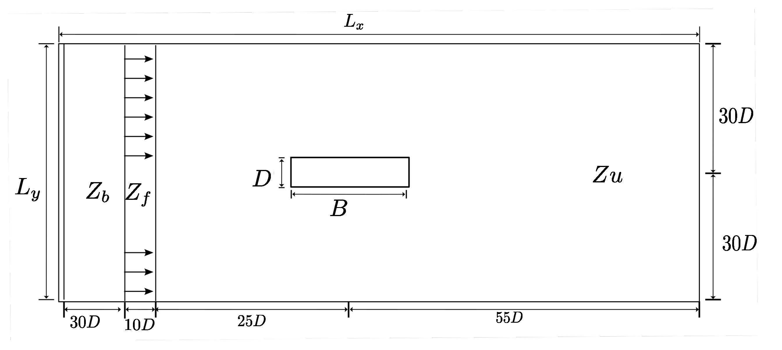
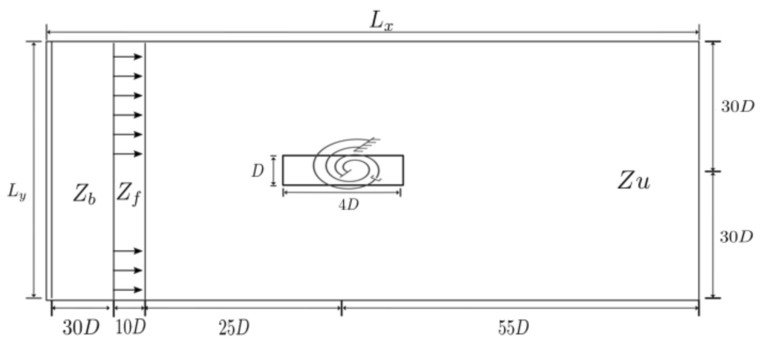
3.2. Numerical Modeling

3.2.1. Fourier Transform in Fluid Modeling

The numerical modeling is performed using FPM [25,26,27], transforming the velocity and pressure fields to a Fourier spectral space. The main advantage of this transformation is that it simplifies some mathematical operations in the spectral domain and, usually, converts a partial differential equation into an ordinary differential equation. In contrast, other operations become more complex, such as the product of two functions, as detailed in Briggs and Henson [28]. In this study, the Fourier transform algorithm, proposed by Takahashi [29], is applied to Equations (1) and (2).

Applying the Fourier transform to Equation (1), Equation (9) is obtained:

$$\iota k_j\widehat{u_j}=0,$$

(9)

where $\iota =\sqrt{-1}$ is the imaginary number and k is the wave number vector, which is orthogonal to the transformed velocity field $\widehat{u(\overrightarrow{k},t)}$. This procedure defines the divergence-free plane, denoted as plane $\pi$.

Applying the same procedure to Equation (2), Equation (10) is obtained:

$${\displaystyle \frac{\partial {\widehat{u}}_i}{\partial t}}+\iota k_j\widehat{u_i{u}_j}=-\iota k_i\widehat{p}-\nu k^2{\widehat{u}}_i+{\widehat{f}}_i,$$

(10)

where $\nu$ is the kinematic viscosity and $k^2$ is the squared norm of the wave number vector, i.e., $k^2=k_j{k}_j$.

All terms in Equation (10) must be projected in the plane $\pi$ to ensure mass balance. Thus, $-\iota k_i\widehat{p}$ is collinear to the vector $\left(\overrightarrow{k}\right)$, i.e., the pressure term can be separated from the velocity solution. Therefore, the FPM did not use the pressure–velocity coupling [19]. The time integration to solve Equations (10) and (8) is performed by the fourth-order Runge–Kutta method using six steps. Nascimento et al. [1,30,31], Mariano et al. [32,33], Kinoshita et al. [34,35], Albuquerque et al. [36], Villela et al. [37], and Monteiro and Mariano [38] detailed this methodology, validation, verification, and application.

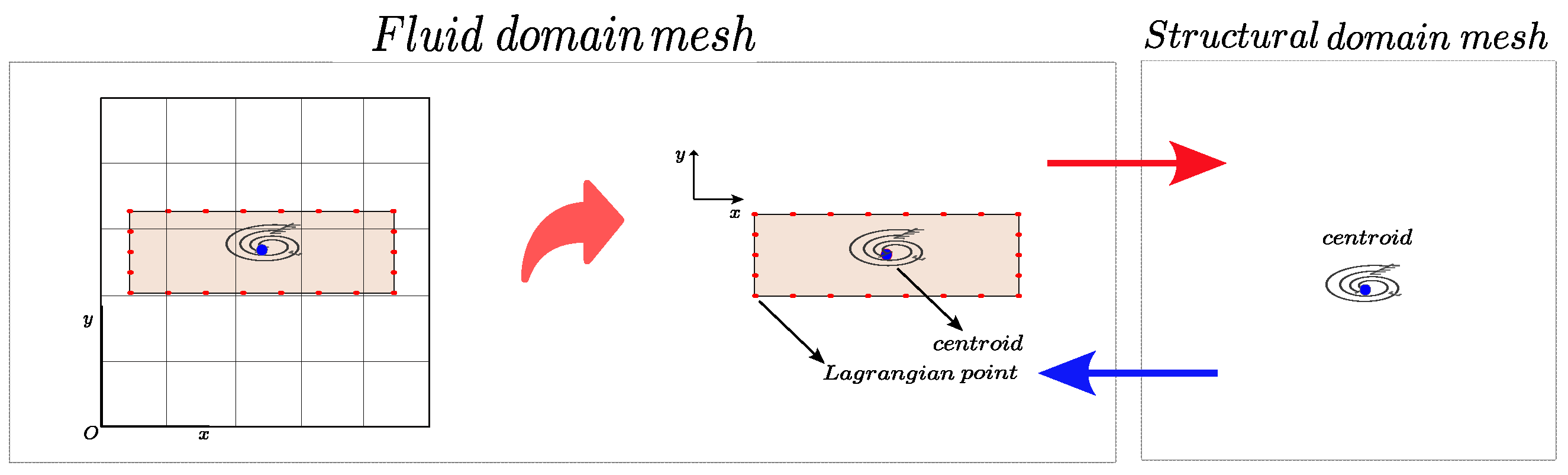
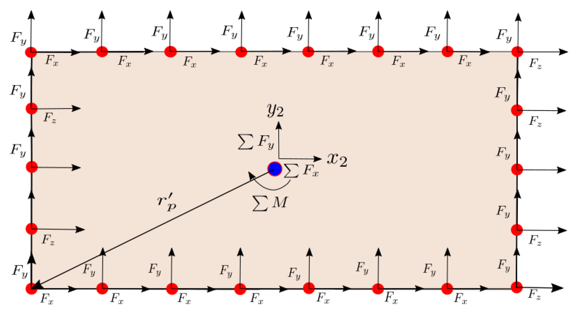
3.2.2. Fluid–Structure Coupling

The constitutive and equilibrium or motion equations, established by fundamental principles of dynamics, applying appropriate adjustments, are valid for fluids and structures. This is the basis for the approach used in Continuum Mechanics. However, the different characteristics between the discretized equations describing the flow and those describing the structure motion are a key challenge in solving FSI problems. The discretization of these two systems of equations results in linear systems with a large number of equations with high sparsity, making the solution difficult. This approach is known as Simultaneous or Monolithic, and its main characteristic is the simultaneous progression of all domains [39].

Another approach involves distinct and independent procedures for solving fluid dynamics and solid mechanics problems, with the coupling achieved through the bidirectional information exchange of kinematic and dynamic data. Figure 3 shows that the mesh in these two systems is different, the Lagrangian points define the immersed body (in red), and the centroid represents the structure domain.

Thus, the forces and momentum exerted by the fluid on the rectangular cylinder surface, calculated through IBM, must be transferred to the node of the structural mesh. In addition, displacements and velocities must be transferred to the rectangular cylinder surface in contact with the fluid.

In this study, the cross-section of the rectangular cylinder is associated with a node of the structural mesh in which the force and momentum applied to the node are the sum of the loads acting on all nodes of the Lagrangian mesh along the rectangular cylinder surface, as illustrated in Figure 4. The red points represent the Lagrangian points of the immersed body, and the blue points indicate the node of the structural mesh.

Auxiliary reference axes were used to ease the information exchange between these two domains. This mathematical modeling used three axes. The $O_{xy}$ and $A_{x_1{y}_1}$ axes were fixed and rigidly positioned at the initial of the domain and centroid, respectively, while the $A_{x_2{y}_2}$ axis moved together with the cross-section of the rectangular cylinder. Figure 5 shows this configuration.

The orthogonal system $A_{x_2{y}_2}$ has a single rotational degree of freedom about the z-axis defined from the structural motion equation (Equation (8)) for the position and angular velocity of the centroid, which can be represented by $\theta$ and $\omega ={\displaystyle \frac{\mathrm{d}\theta }{\mathrm{d}t}}$. This system behaves as a rigid body, which implies that the distance between two points within it remains unchanged during the motion. The position of the Lagrangian point on the moving axis $\left(A_{x_2{y}_2}\right)$ is defined as $r_p^{\prime }$ for p = 1 to p = Np, where Np represents the total number of Lagrangian points. Since the system is plane, the Lagrangian forces at each point are given by $F(X,t)=F_x\left(t\right)+F_y\left(t\right)$, as presented in Figure 4. Similarly, Lagrangian forces can be defined as

$${\left(F\right)}_{Oxy}=\sum _{p=1}^n{F}^p(\overrightarrow{X},t),$$

(11)

where ${\left(F\right)}_{Oxy}$ is the sum of Lagrangian forces in the inertial reference frame $O_{xy}$. The direction of the $A_{x_1{y}_1}$ axis system is observed to remain unchanged relative to the inertial reference frame $O_{xy}$. Thus, they can be applied directly to the node of the structural mesh without any transformation.

$$\left(F_{x_1{y}_1}\right)={\left(F\right)}_{Oxy}.$$

(12)

Figure 5 shows that the vector $\left(r_{B/A}^p\right)$ is the position at the p-th Lagrangian point in the $A_{x_1{y}_1}$ axis. However, the Lagrangian points are defined by $r_p^{\prime }$ in the reference system $A_{x_2{y}_2}$. Since the Lagrangian forces are represented in the $A_{x_1{y}_1}$ axis, The projection of the vector $r_p^{\prime }$ was carried out in this coordinate system due to its directions being constant and parallel to the inertial reference frame. This projection is performed using a rotation matrix defined based on Euler angles. In this case, it consists of a rotation by an angle $\theta$ about the z-axis, described by the following matrix form:

$$T=\left[\begin{array}{ccc}cos\left(\theta \right)& -sin\left(\theta \right)& 0\\ sin\left(\theta \right)& cos\left(\theta \right)& 0\\ 0& 0& 1\end{array}\right]$$

(13)

Thus, the following was obtained:

$${\left(M\right)}_{A_{x_1{y}_1}}=\sum _{p=1}^n[T{\left(r_p^{\prime }\right)}_{A_{x_2{y}_2}}\times F^p(\overrightarrow{X},t)].$$

(14)

Therefore, forces and momentum are applied to the node of the structural mesh and used as input data in this model. After completing the calculations in the structural model, the new position and velocity are transferred to the Eulerian mesh. Figure 5 shows that the new position of the Lagrangian points is given by

$$\left(r_B^p\right)=r_A+r_{B/A}^p$$

(15)

After defining the new coordinates of the Lagrangian points, the velocity of the Lagrangian points must be updated. This procedure is crucial since it directly influences the Lagrangian force calculation and the behavior of the flow over the immersed body. Thus, performing the time derivative of Equation (15) and considering ${\displaystyle \frac{\mathrm{d}\left(r_A\right)}{\mathrm{d}t}}=0$, the following was obtained:

$$U_p^{FI}={\left({\displaystyle \frac{\mathrm{d}\left(r_B^p\right)}{\mathrm{d}t}}\right)}_{O_{xy}}=\omega \times {\left(r_{B/A}^p\right)}_{A_{x_1{y}_1}},$$

(16)

where $U_p^{FI}$ is the velocity of the p-th Lagrangian point.

4. Simulation Results

All the results presented in this study refer to a laminar flow regime, considering a Newtonian and incompressible fluid. The assumptions of laminar behavior ensure that the flow remains orderly and predictable throughout the simulations, allowing for accurate identification of the dynamic responses of the immersed structure. Moreover, the Newtonian nature of the fluid implies a linear relationship between shear stress and strain rate, while the incompressibility assumption simplifies the governing equations by neglecting density variations.

The results are discussed in terms of the dimensionless coefficients of drag, lift, and moment, which are essential for characterizing the hydrodynamic behavior of the body under fluid flow. These coefficients are defined as follows:

$$C_D={\displaystyle \frac{F_D}{\frac{1}{2}\rho u_{\infty }^{2}D}},C_L={\displaystyle \frac{F_L}{\frac{1}{2}\rho u_{\infty }^{2}D}},C_M={\displaystyle \frac{M}{\frac{1}{2}\rho u_{\infty }^2{D}^2}}$$

(17)

where $C_D$ is the drag coefficient, $C_L$ is the lift coefficient, and $C_M$ is the moment coefficient. In these expressions, $F_D$ and $F_L$ represent the drag and lift forces acting on the body, respectively; and M is the moment around the center of mass, which in this case corresponds to the unit length of the cylinder. These non-dimensional parameters allow for a consistent comparison of results under different flow and geometric conditions, and provide insight into the flow-induced forces and dynamic behavior of the system.

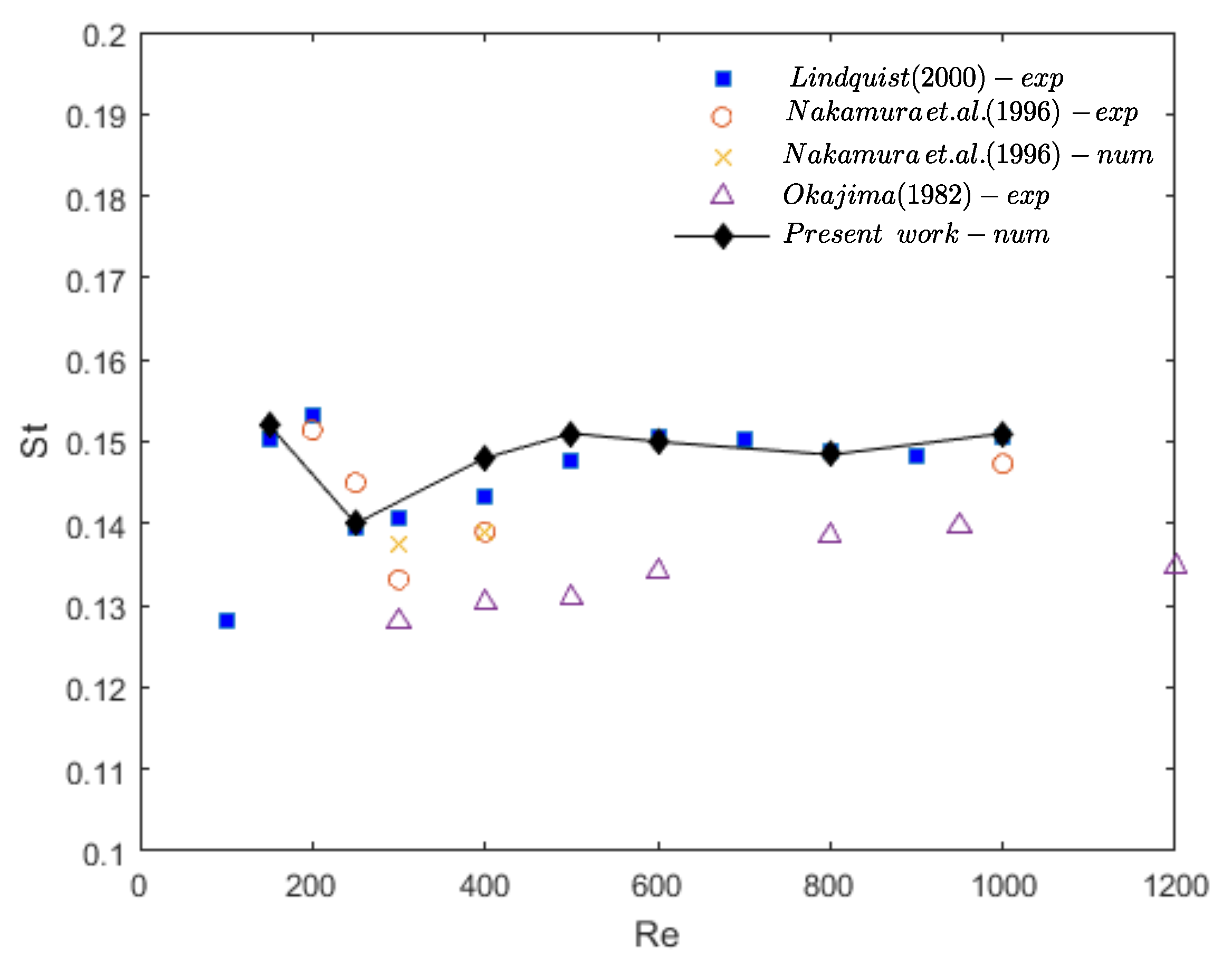
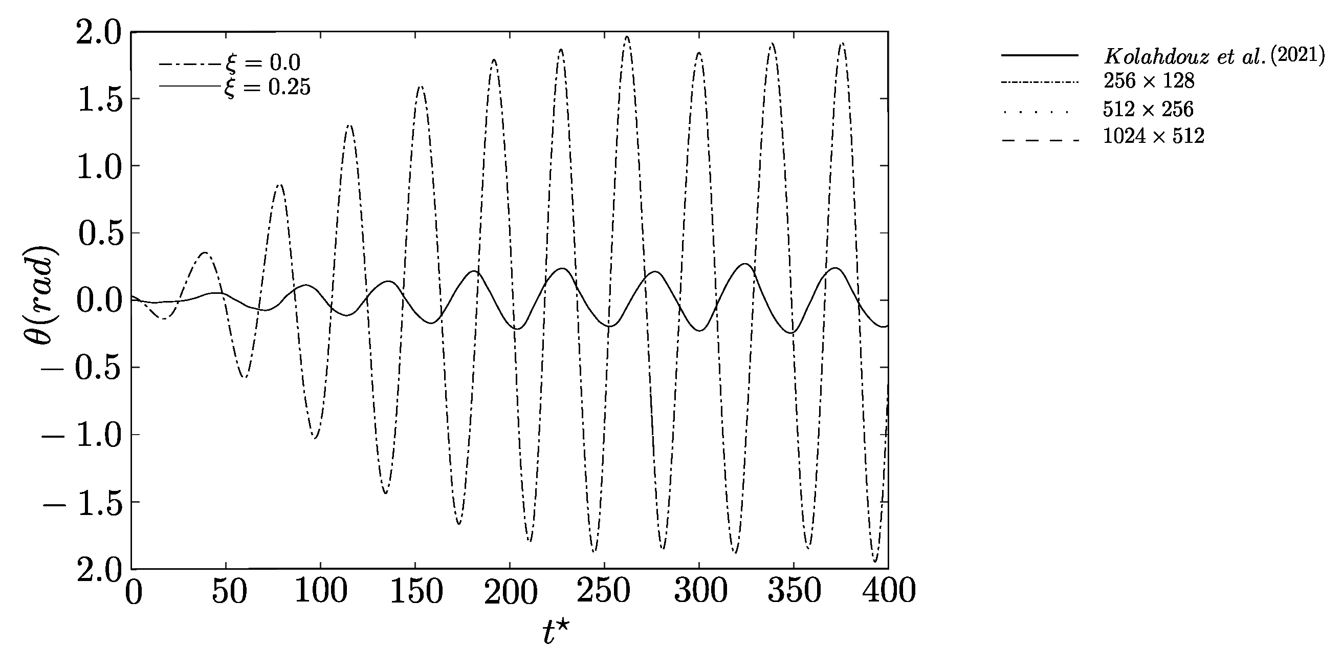
4.1. Numerical Validation

Figure 6 presents the flow over the rectangular cylinder, characterized by the aspect ratio $\varphi ={\displaystyle \frac{B}{D}}$, where D is the cylinder height and B is the cylinder length [40,41,42]. It also indicates that the total domain ($L_x\times L_y$) is divided into three zones, i.e., buffer zone ($Z_b$), forcing zone ($Z_f$), and physical zone ($Z_u$).

Table 2. Simulation parameters.

Description	Symbols	Values
Rectangle height (cm)	D	1
Rectangle base (cm)	B	4
Maximum velocity (cm/s)	$u_{\infty }$	1
Domain dimensions	$L_x\times L_y$	$120D\times 60D$
Density (${\mathrm{kg}/\mathrm{m}}^3$)	$\rho$	1000
Courant number	CFL	0.01
Dimensionless final time	${\displaystyle \frac{t{u}_{\infty }}{D}}$	400

details the parameters considered. The numerical validation considered $Re={\displaystyle \frac{u_{\infty }D}{\nu }}$= 150, 250, 400, 500, 600, 800, and 1000 using a mesh refinement in the Eulerian domain of 256 × 128, 512 × 256, and 1024 × 512, and the number of Lagrangian points of $N_l$ = 21, 44, and 85, respectively.

Figure 7a shows the drag and lift coefficients as a function of time for $D/B=4.0$. It can be observed that the flow was stabilized after 200, with average values of $C_d=1.11$ and $C_d=1.10$ for $512\times 256$ and $1024\times 512$ meshes, respectively. Upon analyzing these mesh refinements in Figure 7b, it can be observed that the signal exhibits a periodic behavior.

The refinement of the Eulerian domain has a direct impact on the behavior of the aerodynamic coefficients $C_l$ and $C_d$, resulting in increased accuracy in their estimation. It is evident that the 256 × 128 mesh lacks sufficient resolution to accurately capture the variations in these coefficients, especially when compared to finer mesh levels. This highlights the importance of mesh refinement in achieving numerically accurate results.

Table 3. Comparison of various approaches for the Strouhal number ($St$).

Reference	Approach	St
Nakamura et al. [41]	Experimental	0.145
Lindquist [40]	Experimental	0.139
Present study	Theoretical/256 × 128	0.010
Present study	Theoretical/512 × 256	0.140
Present study	Theoretical/1024 × 512	0.146

presents the Strouhal numbers ($St={\displaystyle \frac{f_{n}D}{U}}$); f is the vortex shedding frequency (Hz) for Re = 250. It can be observed that the 256 × 128 mesh cannot be used to represent the coefficients, whereas the 512 × 256 and 1024 × 512 meshes achieved values that are closer to those reported in the literature. The Strouhal number reported by Nakamura et al. [41] differed by 0.68%, i.e., lower than 1%, compared to this study for the 1024 × 512 mesh. Comparing the Strouhal number obtained by Lindquist [40], the difference was 5% and 0.7% for 1024 × 512 and 512 × 256 meshes, respectively.

Figure 8 shows that the mesh refinement, domain size, and other parameters were suitably selected to capture the complex wake dynamics, characterized by abrupt changes in the Strouhal number. As expected, the results for 512 × 256 mesh were close to the experimental results reported by Lindquist [40] for $Re=150,250,600,800,$ and 1000.

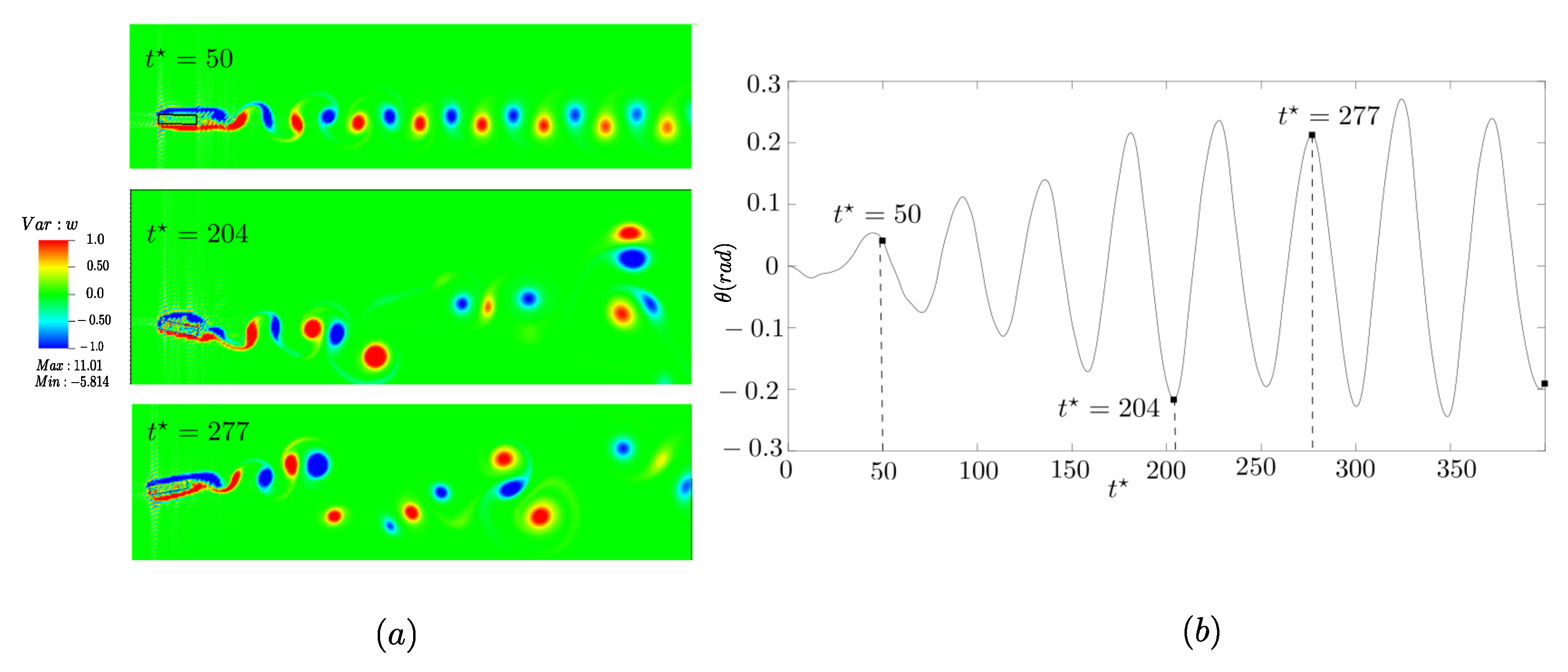
4.2. Galloping Phenomenon

According to Nakamura [43], galloping is a flutter phenomenon that occurs in a single degree of freedom of a bluff body in translational motion orthogonal to the flow direction. Figure 9 shows the physical domain simulated with Cartesian dimensions similar to Figure 6 and using the following parameters: reduced velocity ($U_r=40$); ratio of the moment of inertia ($n_{\theta }=400)$; structural damping ratio (${\zeta }_{\theta }=0$ and ${\zeta }_{\theta }=0.25$); $Re=250$; fluid density ($\rho =1000{\mathrm{kg}/\mathrm{m}}^3$); flow velocity ($u_{\infty }$ = 1.0 cm/s); $N_x$ × $N_y$ = 256 × 128, 512 × 256, and 1024 × 512; CFL = 0.01; and $t^{★}=400$.

Figure 10 presents the time evolution of the oscillation amplitude of the rectangular cylinder, defined by the rotation angles that the structure reaches relative to its equilibrium position as a function of time. The time evolution for the 256 × 128 mesh from $t^{★}=200$ did not oscillate, showing a smooth behavior. For the 512 × 256 mesh, the oscillation frequency and maximum amplitude were $f_o=0.018{\mathrm{s}}^{-1}$ and $\theta =0.24$ (rad), respectively. These values differ from Kolahdouz et al. [24] by 9.1% (oscillation frequency) and 8.3% (maximum amplitude). In the 1024 × 512 mesh, the oscillation frequency and maximum amplitude were $f_o=0.020s^{-1}$ and ${\theta }_{max}=0.27$ (rad), respectively. These values are close to those by Kolahdouz et al. [24].

Table 4. Maximum amplitude and frequency ratio.

Reference	$\mathit{\theta }$ (rad)	${\mathit{f}}_{\mathit{o}}/{\mathit{f}}_{\mathit{n}}$
Robertson et al. [9]	0.262	0.762
Dettmer and Perić [21]	0.267	0.800
Yang and Stern [10]	0.274	0.792
He et al. [23] Semi-implicit	0.310	0.805
Yang et al. [22]	0.281	0.788
Kolahdouz et al. [24]	0.262	0.792
Present work: 512 × 256	0.240	0.736
Present work: 1024 × 512	0.272	0.800

compares the properties related to the “galloping” phenomenon, i.e., $\theta$ and $f_o/f_n$ for $Re=250$, with those from references [9,10,21,22,23,24]. The authors agree that a more precise analysis could be conducted using nonlinear methods for the immersed structural rotation angle. However, it has been observed that considering sin($\theta$) equal to $\theta$ for 0.24 radians results in only a 0.96% error. Furthermore, it is noteworthy that the references found in the literature and used to validate the present methodology employed linear systems, including Robertson et al. [9], Yang and Stern [10], Dettmer and Perić [21], Yang et al. [22], He et al. [23], and Kolahdouz et al. [24].

Figure 11 shows that the lift coefficient ($C_l$) exhibits two dominant frequencies: one corresponding to the structural vibration frequency and the other close to the vortex shedding frequency of the fixed geometry under analysis. This indicates the occurrence of the galloping phenomenon at $Re=250$, for flow over a rectangular cylinder with $\varphi$ = 4, mounted on a torsional spring, where the response is associated with vortex shedding. This dynamic behavior, characterized by the coexistence of the structural vibration frequency and the vortex shedding frequency, suggests a coupling mechanism that may lead to dynamic instability such as galloping. The presence of significant oscillatory amplitudes in both the structural response and lift coefficient is an indicator of the proximity to a critical condition.

Figure 12 presents the wake dynamics for $\varphi =4$, $Re=250$, and $U_r=40$ with vorticity varying from −1.0 to 1.0. For $t^{★}=50$, the wake pattern is identified by 2S, i.e., the shedding of only one vortex on each side can be observed, along with a very low displacement amplitude. This wake pattern modifies when the structure moves. This is evident at $t^{*}=204$, when the geometry starts moving upwards, and $t^{*}=277$, when the geometry starts moving downwards, corresponding to $\theta =0.21$ radians, or ${12}^{\circ }$, near the rotational peak.

In Figure 13, the draft coefficient ($C_d$) at $t^{★}=50$ oscillated with low amplitude, around $C_d=1$. The amplitude of these oscillations gradually increased by increasing $t^{*}$. For $t^{*}>200$, it exhibits an unstable and irregular behavior over time, suggesting a nonlinear dynamic response to the flow, with instability releases. The momentum ($C_m$) and lift ($C_l$) coefficients for $t^{★}>150$ indicated that the lift force contributed to the rotational structure instability, highlighted by the sharp increase in $C_l$ and the sharp decrease in $C_d$. This suggests a dynamic interaction between the transverse and rotational oscillation modes of the structure, which is also observed by Robertson et al. [9]. Galloping frequency was $f_o=0.020{\mathrm{s}}^{-1}$ in agreement with Kolahdouz et al. [24].

Figure 14 shows the rotational structure motion throughout $t^{★}=400$. The system oscillations with slowly increasing amplitude stabilized at $t^{*}=200$. The system modeled with ${\zeta }_{\theta }=0$ had the highest oscillation amplitude, around eight times higher, than the system with ${\zeta }_{\theta }=0.25$, which oscillated with reduced frequency. Yang and Stern [10] reported a similar behavior.

5. Conclusions

Our previous studies verified and validated that the IMERSPEC2D numerical code was developed [1,30,31]. This study is an extension to investigate the behavior of a rectangular cylinder with an aspect ratio $\varphi$ of 4. A rigid body was modeled using the dimensionless technique applied to the structural model. The proposed formulation used time increments of ${10}^{-2}$ and ${10}^{-3}$.

The mesh refinement results demonstrated the potential of the IMERSPEC methodology since the 512 × 256 mesh, i.e., 131,072 collocation points, did not significantly change the Strouhal number St. This indicates that the method can avoid memory overhead with low computational cost.

In addition, investigating the flow over a rectangular cylinder enabled an in-depth understanding of the wake pattern of turbulent structures generated during FSI. The detailed analysis showed the complexity and dynamics of these phenomena, providing significant insight into vortex formation and the nature of the aerodynamic forces involved. Furthermore, the results show a spatial symmetry breaking in the flow patterns, while the oscillatory motion of the rigid body preserves temporal symmetry, reinforcing the robustness of the IMERSPEC methodology in capturing space–time symmetry behaviors. The 512 × 256 mesh allowed us to evaluate the torsional boundary condition using IBM, showing the efficiency and stability of the methodology.

Although a complete parametric stability analysis is beyond the scope of this study, the current result demonstrates a condition where instability mechanisms emerge, providing a reference for identifying unstable regimes in future work. The observed dynamic response highlights the sensitivity of the system to flow-induced excitations at this Reynolds number. The simultaneous presence of structural and vortex shedding frequencies in the lift coefficient response confirms the FSI. This behavior reinforces the importance of considering both structural and fluid dynamic interactions in the design and analysis of bluff body configurations. The indication of galloping, driven by this coupling, points to a critical operational regime that requires careful evaluation to prevent undesirable vibrations or potential structural failure.

References

1. Nascimento, A.; Mariano, F.; Padilla, E.; Silveira Neto, A. Comparison of the convergence rates between Fourier pseudo-spectral and finite volume method using Taylor-Green vortex problem. J. Braz. Soc. Mech. Sci. Eng. 2020, 42, 491. [Google Scholar] [CrossRef]
2. Peskin, C. Numerical analysis of blood flow in the heart. J. Comput. Phys. 1977, 25, 220–252. [Google Scholar] [CrossRef]
3. Newman, J.N. Marine Hydrodynamics; MIT Press: Cambridge, MA, USA, 1977. [Google Scholar]
4. Faltinsen, O.M. Sea Loads on Ships and Offshore Structures; Cambridge University Press: Cambridge, UK, 1990. [Google Scholar]
5. Chakrabarti, S.K. Handbook of Offshore Engineering; Elsevier: Oxford, UK, 2005. [Google Scholar]
6. Meriam, J.L.; Kraige, L.G. Engineering Mechanics: Dynamic; Wiley: New York, NY, USA, 1990. [Google Scholar]
7. Zhang, G.; Luo, J.; Sun, M.; Yu, Y.; Chen, J.; Wang, J.; Zhang, Z. A novel, reliable parametric model for predicting the nonlinear hysteresis phenomenon of composite magnetorheological fluid. Smart Mater. Struct. 2025, 34, 035060. [Google Scholar] [CrossRef]
8. Li, L.; Sherwin, S.; Bearman, P. A moving frame of reference algorithm for fluid/structure interaction of rotating and translating bodies. Int. J. Numer. Methods Fluids 2002, 38, 187–206. [Google Scholar] [CrossRef]
9. Robertson, I.; Li, L.; Sherwin, S.; Bearman, P. A numerical study of rotational and transverse galloping rectangular bodies. J. Fluids Struct. 2003, 17, 681–699. [Google Scholar] [CrossRef]
10. Yang, J.; Stern, F. A simple and efficient direct forcing immersed boundary framework for fluid–structure interactions. J. Comput. Phys. 2012, 231, 5029–5061. [Google Scholar] [CrossRef]
11. Yang, J.; Stern, F. A non-iterative direct forcing immersed boundary method for strongly-coupled fluid–solid interactions. J. Comput. Phys. 2015, 295, 779–804. [Google Scholar] [CrossRef]
12. Nomura, T. Finite element analysis of vortex-induced vibrations of bluff cylinders. In Computational Wind Engineering 1; Murakami, S., Ed.; Elsevier: Oxford, UK, 1993; pp. 587–594. [Google Scholar] [CrossRef]
13. Cui, Z.; Zhao, M.; Teng, B.; Cheng, L. Two-dimensional numerical study of vortex-induced vibration and galloping of square and rectangular cylinders in steady flow. Ocean Eng. 2015, 106, 189–206. [Google Scholar] [CrossRef]
14. Siriyothai, P.; Kittichaikarn, C. Performance enhancement of a galloping-based energy harvester with different groove depths on square bluff body. Renew. Energy 2023, 210, 148–158. [Google Scholar] [CrossRef]
15. Hémon, P.; Amandolese, X.; Andrianne, T. Energy harvesting from galloping of prisms: A wind tunnel experiment. J. Fluids Struct. 2017, 70, 390–402. [Google Scholar] [CrossRef]
16. Uhlmann, M. An immersed boundary method with direct forcing for the simulation of particulate flows. J. Comput. Phys. 2005, 209, 448–476. [Google Scholar] [CrossRef]
17. Tornberg, A.K.; Engquist, B. Numerical approximation of singular source in differential equations. J. Comput. Phys. 2004, 200, 462–488. [Google Scholar] [CrossRef]
18. Luo, H.; Dai, H.; Ferreira de Sousa, P.J.; Yin, B. On the numerical oscillation of the direct-forcing immersed-boundary method for moving boundaries. Comput. Fluids 2012, 56, 61–76. [Google Scholar] [CrossRef]
19. Kim, J.; Kim, D.; Choi, H. An Immersed-Boundary Finite-Volume Method for Simulations of Flow in Complex Geometries. J. Comput. Phys. 2001, 171, 132–150. [Google Scholar] [CrossRef]
20. Takizawa, K.; Tezduyar, T.E. Computational methods for fluid–structure interaction with the space–time formulations. J. Syst. Des. Dyn. 2003, 16, 571–572. [Google Scholar] [CrossRef]
21. Dettmer, W.; Perić, D. A computational framework for fluid–rigid body interaction: Finite element formulation and applications. Comput. Methods Appl. Mech. Eng. 2006, 195, 1633–1666. [Google Scholar] [CrossRef]
22. Yang, X.; Sotiropoulos, F.; Conzemius, R.J.; Wachtler, J.N.; Strong, M.B. Large-eddy simulation of turbulent flow past wind turbines/farms: The Virtual Wind Simulator (VWiS). Wind Energy 2015, 18, 2025–2045. [Google Scholar] [CrossRef]
23. He, T.; Zhou, D.; Han, Z.; Tu, J.; Ma, J. Partitioned subiterative coupling schemes for aeroelasticity using combined interface boundary condition method. Int. J. Comput. Fluid Dyn. 2014, 28, 272–300. [Google Scholar] [CrossRef]
24. Kolahdouz, E.M.; Bhalla, A.; Scotten, L.; Craven, B.; Griffith, B. A sharp interface Lagrangian-Eulerian method for rigid-body fluid-structure interaction. J. Comput. Phys. 2021, 443, 110–442. [Google Scholar] [CrossRef]
25. Canuto, C.; Hussaini, M.; Quarteroni, A.; Zang, T. Spectral Methods: Fundamentals in Single Domains; Scientific Computation; Springer: Berlin/Heidelberg, Germany, 2006. [Google Scholar]
26. Canuto, C.; Hussaini, M.; Quarteroni, A.; Thomas A., J. Spectral Methods in Fluid Dynamics; Scientific Computation; Springer: Berlin/Heidelberg, Germany, 1988. [Google Scholar]
27. Canuto, C.; Hussaini, M.; Quarteroni, A.; Zang, T. Spectral Methods: Evolution to Complex Geometries and Applications to Fluid Dynamics; Springer: Berlin/Heidelberg, Germany, 2007. [Google Scholar]
28. Briggs, W.; Henson, V. The DFT: An Owners’ Manual for the Discrete Fourier Transform; Other Titles in Applied Mathematics; Society for Industrial and Applied Mathematics: Philadelphia, PA, USA, 1995. [Google Scholar]
29. Takahashi, D. A Hybrid MPI/OpenMP Implementation of a Parallel 3-D FFT on SMP Clusters; Springer: Berlin/Heidelberg, Germany, 2006; pp. 970–977. [Google Scholar] [CrossRef]
30. Nascimento, A.A.; Mariano, F.P.; Silveria-Neto, A.; Padilla, E.L.M. A comparison of Fourier pseudospectral method and finite volume method used to solve the Burgers equation. J. Braz. Soc. Mech. Sci. Eng. 2014, 36, 737–742. [Google Scholar] [CrossRef]
31. Nascimento, A.; Mariano, F.; da Silveira Neto, A.; Padilla, E.L.M. Coupling of the immersed boundary and Fourier pseudo-spectral methods applied to solve fluid–structure interaction problems. J. Braz. Soc. Mech. Sci. Eng. 2024, 46, 213. [Google Scholar] [CrossRef]
32. Mariano, F.P.; Moreira, L.d.Q.; Nascimento, A.A.; Silveira-Neto, A. An improved immersed boundary method by coupling of the multi-direct forcing and Fourier pseudo-spectral methods. J. Braz. Soc. Mech. Sci. Eng. 2022, 44, 388. [Google Scholar] [CrossRef]
33. Mariano, F.P.; Moreira, L.d.Q.; Silveira-Neto, A.d.; da Silva, C.B.; Pereira, J.C. A new incompressible Navier-Stokes solver combining Fourier pseudo-spectral and immersed boundary methods. Comput. Model. Eng. Sci. 2010, 59, 181–216. [Google Scholar] [CrossRef]
34. Kinoshita, D.; Martínez Padilla, E.L.; da Silveira Neto, A.; Pamplona Mariano, F.; Serfaty, R. Fourier pseudospectral method for nonperiodical problems: A general immersed boundary method for three types of thermal boundary conditions. Numer. Heat Transf. Part B Fundam. 2016, 70, 537–558. [Google Scholar] [CrossRef]
35. Kinoshita, D.; da Silveira Neto, A.; Mariano, F.P.; da Silva, R.A.P.; Serfaty, R. A novel immersed boundary/Fourier pseudospectral method for flows with thermal effects. Numer. Heat Transf. Part B Fundam. 2016, 69, 312–333. [Google Scholar] [CrossRef]
36. Albuquerque, L.; Villela, M.; Mariano, F. Numerical Simulation of Flows Using the Fourier Pseudospectral Method and the Immersed Boundary Method. Axioms 2024, 13, 228. [Google Scholar] [CrossRef]
37. Villela, M.; Villar, M.; Serfaty, R.; Mariano, F.; Silveira-Neto, A. Mathematical modeling and numerical simulation of two-phase flows using Fourier pseudospectral and front-tracking methods: The proposition of a new method. Appl. Math. Model. 2017, 52, 241–254. [Google Scholar] [CrossRef]
38. Monteiro, L.; Mariano, F. Flow Modeling over Airfoils and Vertical Axis Wind Turbines Using Fourier Pseudo-Spectral Method and Coupled Immersed Boundary Method. Axioms 2023, 12, 212. [Google Scholar] [CrossRef]
39. Farhat, C.; Lessoinne, M.; Letallec, P. Load and motion transfer algorithms for fluid/structure interaction problems with non-matching discrete interfaces: Momentum and Energy conservation, optimal discretization and application to aeroeslaticity. Comput. Methods Appl. Mech. Eng. 1998, 157, 98–114. [Google Scholar] [CrossRef]
40. Lindquist, C. Estudo Numérico e Experimental do Escoamento ao Redor de Cilindros de Base Quadrada e Retangular. Master’s Thesis, Universidade Estadual Paulista, São Paulo, Brazil, 2000. [Google Scholar]
41. Nakamura, Y.; Ohya, Y.; Ozono, S.; Nakayama, R. Experimental and numerical analysis of vortex shedding from elongated rectangular cylinders at low Reynolds numbers 200-103. J. Wind Eng. Ind. Aerodyn. 1996, 65, 301–308. [Google Scholar] [CrossRef]
42. Okajima, A. Strouhal numbers of rectangular cylinders. J. Fluid Mech. 1982, 123, 379–398. [Google Scholar] [CrossRef]
43. Nakamura, Y. Recent research into bluff-body flutter. J. Wind Eng. Ind. Aerodyn. 1990, 33, 1–10. [Google Scholar] [CrossRef]
Figure 1. Schematic representation of the computational domains used in the immersed boundary method. The sketch illustrates the Eulerian grid (fluid domain) and the Lagrangian mesh (solid boundary), highlighting their interaction regions. This configuration allows the enforcement of boundary conditions on complex geometries immersed in the flow field.
Symmetry 17 01142 g001
Figure 2. Schematic of the two-dimensional rigid body immersed in a Cartesian computational grid. The body, represented as a rectangular structure, is anchored at point A and allowed to rotate about this point under the influence of fluid forces. Three auxiliary reference axes were defined: The global O x y and the local A x 1 y 1 axes were fixed at the domain origin and at the body’s centroid, respectively, while the A x 2 y 2 axis translated with the rectangular cylinder’s cross section. Point B denotes the Lagrangian point.
Symmetry 17 01142 g002
Figure 3. Scheme of fluid–structure coupling via Lagrangian points. The structure immersed in the fluid domain is represented by Lagrangian points (in red), which facilitate the exchange of information between the domains. On the right is the structural reference point, where the rigid body forces and moments are concentrated at structural centroid (blue point). The red arrow indicates the transfer of loads from the fluid to the structure, while the blue arrow represents the feedback of structural displacements and angular velocity to the fluid, characterizing the bidirectional coupling.
Symmetry 17 01142 g003
Figure 4. Transfer of Lagrangian forces to the structural reference point of the immersed rigid body, where the distribution of Lagrangian forces ( F x , F y ) is applied at discrete interface points (red dots) on the surface of the immersed body. These forces are summed and transferred to the structural reference point (blue dot), where the total resultant forces ( F x , F y ) and the resultant moment ( M ) are computed. The vector r p represents the position vector from the reference point to a generic Lagrangian force application point. This process ensures the consistent and accurate coupling of fluid-induced loads to the dynamics of the rigid body structure.
Symmetry 17 01142 g004
Figure 5. Schematic of the two-dimensional rigid body immersed in a Cartesian computational grid. The body, represented as a rectangular structure, is anchored at point G, the center of mass, and allowed to rotate (angle θ ) about this point under the influence of fluid forces. This configuration is used to study fluid–structure interaction using the immersed boundary method.
Symmetry 17 01142 g005
Figure 6. Domain configuration used for validating the flow around a fixed rectangular body. This setup serves as a reference for comparison with cases involving fluid–structure interaction, ensuring consistency and accuracy in the numerical implementation before introducing body motion.
Symmetry 17 01142 g006
Figure 7. Time evolution of the coefficients as a function of dimensionless time for R e = 250 : the solid blue line represents the results obtained using the 256 × 128 mesh, the solid red line corresponds to the 512 × 256 mesh, and the solid black line denotes the results from the 1024 × 512 mesh. (a) C d and (b) C l .
Symmetry 17 01142 g007
Figure 8. Strouhal number as a function of Reynolds number for a rectangular cylinder with aspect ratio ϕ = 4 , computed using the 512 × 256 mesh. Numerical results from the present study (solid black line with diamonds) are compared with experimental data from Lindquist [40], Nakamura et al. [41] and Okajima [42].
Symmetry 17 01142 g008
Figure 9. Illustration of the computational setup for the fluid–structure interaction problem. The figure highlights the placement of the oscillating rectangular body within the flow domain and the division into subregions used for boundary condition definition and flow analysis.
Symmetry 17 01142 g009
Figure 10. Temporal evolution of the angular displacement θ for a freely rotating rectangular body at R e = 250 , expressed in nondimensional time. reduced velocity U r = 40 , and angular discretization n θ = 400 (Kolahdouz et al. [24]).
Symmetry 17 01142 g010
Figure 11. Analysis of C L and θ for U r = 40 , using a 1024 × 512 mesh: (a) time history expressed in nondimensional time; (b) frequency spectrum obtained from the time signal using Fast Fourier Transform (FFT).
Symmetry 17 01142 g011
Figure 12. The coupling between the wake dynamics and the rotational response of the body. (a) Vorticity 1 w 1 at three selected nondimensional time instants ( t = 50 , 204, and 277) during the flow around a rectangular cylinder with aspect ratio ϕ = 4 . (b) The temporal evolution of the angular displacement θ , with markers indicating the corresponding instants.
Symmetry 17 01142 g012
Figure 13. Temporal evolution of the aerodynamic force and moment coefficients for a freely rotating rectangular cylinder with aspect ratio ϕ = 4 , using nondimensional time. The plots show the time histories of the drag coefficient ( C d ), lift coefficient ( C l ), and moment coefficient ( C m ).
Symmetry 17 01142 g013
Figure 14. Temporal evolution of the rotational angle θ in nondimensional time for two damping ratios, ζ = 0 and ζ = 0.25 , at Reynolds number R e = 250 , reduced velocity U r = 40 , and n θ = 400 . The results illustrate the effect of structural damping on the free rotational motion of the body.
Symmetry 17 01142 g014