Quasi-Periodic Dynamics and Wave Solutions of the Ivancevic Option Pricing Model Using Multi-Solution Techniques

Abstract

In this research paper, we study symmetry groups, soliton solutions, and the dynamical behavior of the Ivancevic Option Pricing Model (IOPM). First, we find the Lie symmetries of the considered model; next, we use them to determine the corresponding symmetry groups. Then, we attempt to solve IOPM by means of two methods. We provide some wave solutions and give further details of the solution using 2D and 3D graphs. These results are interpreted as important clarifications in financial mathematics and deepen our understanding of the dynamics involved during the pricing of options. Secondly, the quasi-periodic behavior of the two-dimensional dynamical system and its perturbed system are plotted using Python software (Python 3.13.5 version). Various frequencies and amplitudes are considered to confirm the quasi-periodic behavior via the Lyapunov exponent, bifurcation diagram, and multistability analysis. These findings are particularly in consonance with current research that investigates IOPM as a nonlinear wave alternate for normal models and the importance of graphical representations in the understanding of financial derivative dynamics. We, therefore, hope to fill in the gaps in the literature that currently exist about the use of multi-solution methods and their effects on financial modeling through the employment of sophisticated graphical techniques. This will be helpful in discussing matters in the field of financial mathematics and open up new directions of investigation.

1. Introduction

In recent years, nonlinear partial differential equations (NLPDEs) [1,2] have been increasingly used to model a wide range of phenomena across physics, chemistry, biology, engineering, and finance [3,4]. For example, in biology, NLPDEs have been applied to describe tumor growth dynamics, while in finance, they have proved valuable for modeling pricing dynamics of financial derivatives such as options and warrants. In physics, the application of NLPDEs is even more extensive, spanning fields like fluid mechanics, quantum mechanics, and plasma physics [5]. Notable examples include the Kaup–Newell Model [6], the fractional stochastic Fokas–Lenells equation [7], the Fractional Magneto-Electro-Elastic System [8], etc. Due to the intricate and highly nonlinear nature of these problems, the study of NLPDEs has become increasingly challenging. In recent years, considerable attention has been devoted to exploring traveling wave solutions and qualitative analyses of NLPDEs, making this area a central focus of research. In this context, the IOPM has emerged as a particularly significant model.

The IOPM was introduced by Dr. Igor Ivancevic. This model presents a novel approach to option pricing that is fundamentally different from the traditional Black–Scholes framework, utilizing concepts from nonlinear dynamics and wave theory. The IOPM [9] is

$$\begin{array}{c}\hfill i{U}_t+{\displaystyle \frac{\mu }{2}}{U}_{ss}+\delta U{\left|U\right|}^2=0·\end{array}$$

(1)

In this context, $U(s,t)$ is a real-valued function that describes the wave dynamics of option prices, where t denotes time and s represents the underlying asset price. The parameter $\mu$ denotes the volatility, while $\delta$ shows the Landau coefficient characterizes the adaptive market potential. As a result, the option price is represented by the associated probability density function $\left(\right|U\left|\right)$. The strength of the IOPM lies in its ability to generate a variety of analytical solutions, making it a highly versatile modeling approach. The IOPM is especially significant because it captures the complexity of financial markets, which often cannot be adequately described using linear models [9]. In the literature, approaches such as the unified auxiliary equation method [10] and the rational sine-Gordon expansion method [11] have been successfully applied to the IOPM, yielding significant insights. This work introduces the following novel aspects: First, we carry out a Lie symmetry analysis of the IOPM and construct its associated symmetry group. Second, we obtain soliton solutions of the model using two distinct methods and graphically depict the results. We then transform the resulting ordinary differential equation (ODE) into a dynamical system and study its behavior, focusing on its chaotic dynamics. The chaos analysis is performed through 2D phase portraits, time–series simulations, and Lyapunov exponents. Notably, this work goes beyond prior studies that have been limited to obtaining solutions and, for the first time explores, the model’s dynamical behavior and its underlying chaos. To further increase their theoretical and practical significance, future studies will focus on extending the scope of these methods, conducting empirical validations, and developing computational algorithms to enable their efficient implementation in financial applications.

A comparison with prior studies in Table 1 highlights the distinct contributions of this work.

Table 1. Comparative analyses.

Current Research	Chen et al. [9] Work
Unified solver method and the $({\displaystyle \frac{1}{\varphi \left(\zeta \right)}},{\displaystyle \frac{{\varphi }^{\prime }\left(\zeta \right)}{\varphi \left(\zeta \right)}})$ method.	Sine-Gordon expansion method.
Investigates chaos analysis using 2D phase portraits, time-series analysis, and Lyapunov exponents.	No chaos analysis performed.
Addresses soliton dynamics and chaos theory.	Focuses mainly on soliton solutions without examining dynamical behavior.

Researchers have developed various methods for obtaining exact solutions to differential equations, among which, Lie group analysis, introduced by Sophus Lie [12], is particularly well known. Inspired by galois theory, Lie formulated a framework that identifies group properties inherent in differential equations, enabling the derivation of analytical solutions. This approach applies to both ordinary and partial differential equations, facilitating the discovery of symmetries. These symmetries are instrumental in finding similarity solutions, conservation laws, and simplifying nonlinear PDEs through linearization, reducing equation order, and minimizing the number of independent variables. The literature explores several types of symmetries, including Lie point symmetries, Noether symmetries, non-classical symmetries, conditional symmetries, approximate and generalized conditional symmetries, and q-conditional symmetries [13].

Solitary wave solutions play a pivotal role in understanding complex nonlinear phenomena across various scientific disciplines. These localized wave structures arise in contexts such as fluid dynamics [14], optical communications [15], plasma physics [16], and biology [17], providing valuable insight into the dynamics, stability, and interactions of nonlinear wave patterns [18]. Due to their ability to retain shape and energy over long distances, solitary wave solutions have become a central focus in nonlinear research. Accordingly, the extraction of solitary wave solutions has become an increasingly captivating subject in the study of NLPDEs. A variety of mathematical methods have been developed to solve NLPDEs, including the Kumar Malik approach [19], the tanh approach [20], the extended hyperbolic function technique [21], etc.

Section 2 discusses the Lie symmetry group of the proposed model. Section 3 presents the methodology employed to derive exact solutions. Section 4 is devoted to the construction of soliton solutions. Section 5 illustrates the graphical representation of the obtained solutions. Section 6 focuses on the chaos analysis of the system. Section 7 concludes the study by summarizing the key findings and outcomes.

2. Lie Analysis

To distinguish between the imaginary and real components of Equation (1), the following assumption is introduced:

$$U(s,t)=\mathcal{R}(s,t)+\iota \mathcal{P}(s,t),$$

(2)

$\mathcal{R}(s,t)$ shows the real parts of the equation, and $\mathcal{P}(s,t)$ represents the imaginary parts of the equation. by substituting Equation (2) into Equation (1), the resulting imaginary and real parts are given by

$$\begin{array}{ccc}\hfill -{\mathcal{P}}_t+\delta \mathcal{R}{\mathcal{P}}^2+\delta {\mathcal{R}}^3+{\displaystyle \frac{\mu }{2}}{\mathcal{R}}_{ss}& =& 0,\hfill \end{array}$$

(3)

$$\begin{array}{ccc}\hfill {\mathcal{R}}_t+\delta \mathcal{P}{\mathcal{R}}^2+\delta {\mathcal{P}}^3+{\displaystyle \frac{\mu }{2}}{\mathcal{P}}_{ss}& =& 0.\hfill \end{array}$$

(4)

Consider the following Lie group of point transformations to obtain the symmetries of system (4):

$$\begin{array}{cc}\hfill & \overline{t}=t+\mathcal{G}\alpha (s,t,\mathcal{R},\mathcal{P})+O\left({\mathcal{G}}^2\right),\hfill \\ \hfill & \overline{s}=s+\mathcal{G}\beta (s,t,\mathcal{R},\mathcal{P})+O\left({\mathcal{G}}^2\right),\hfill \\ \hfill & \overline{\mathcal{R}}=\mathcal{R}+\mathcal{G}\gamma (s,t,\mathcal{R},\mathcal{P})+O\left({\mathcal{G}}^2\right),\hfill \\ \hfill & \overline{\mathcal{P}}=\mathcal{P}+\mathcal{G}\delta (s,t,\mathcal{R},\mathcal{P})+O\left({\mathcal{G}}^2\right).\hfill \end{array}$$

(5)

Here, $\mathcal{G}\ll 1$ with $\alpha ,\beta ,\gamma ,\delta$ as infinitesimals; their extensions follow from the prolongation formulas:

$$\mathcal{F}=\alpha (s,t,\mathcal{R},\mathcal{P}){\displaystyle \frac{\partial }{\partial t}}+\beta (s,t,\mathcal{R},\mathcal{P}){\displaystyle \frac{\partial }{\partial s}}+\gamma (s,t,\mathcal{R},\mathcal{P}){\displaystyle \frac{\partial }{\partial \mathcal{R}}}+\delta (s,t,\mathcal{R},\mathcal{P}){\displaystyle \frac{\partial }{\partial \mathcal{P}}}.$$

(6)

The functions $\alpha ,\beta ,\gamma ,$ and $\delta$ are to be found, and $\mathcal{F}$ satisfies the Lie symmetry condition if and only if this holds:

$${\mathcal{F}}^{\left[2\right]}\left({\mathcal{W}}_e\right){|}_{{\mathcal{W}}_e=0}=0,e=1,2·$$

(7)

where ${\mathcal{W}}_1=-{\mathcal{P}}_t+\delta \mathcal{R}{\mathcal{P}}^2+\delta {\mathcal{R}}^3+{\displaystyle \frac{\mu }{2}}{\mathcal{R}}_{ss},$ and ${\mathcal{W}}_2={\mathcal{R}}_t+\delta \mathcal{P}{\mathcal{R}}^2+\delta {\mathcal{P}}^3+{\displaystyle \frac{\mu }{2}}{\mathcal{P}}_{ss}$. ${\mathcal{F}}^{\left[2\right]}$ represents the second prolongation, and the corresponding formula is

$${\mathcal{F}}^{\left[2\right]}=\mathcal{F}+{\gamma }^s{\displaystyle \frac{\partial }{\partial {\mathcal{R}}_s}}+{\gamma }^{ss}{\displaystyle \frac{\partial }{\partial {\mathcal{R}}_{ss}}}+{\delta }^s{\displaystyle \frac{\partial }{\partial {\mathcal{P}}_s}}+{\delta }^{ss}{\displaystyle \frac{\partial }{\partial {\mathcal{P}}_{ss}}}.$$

(8)

From the prolongations in Equation (7), we derive the Lie symmetry algebra by computing derivatives of the dependent variable. The resulting generators are

$$\begin{array}{cc}\hfill & \alpha =s{\mathcal{C}}_1+t{\mathcal{C}}_2+{\mathcal{C}}_3,\beta =2{\mathcal{C}}_{1}t+{\mathcal{C}}_4,\hfill \\ \hfill & \gamma ={\displaystyle \frac{-\mathcal{P}{C}_{2}s-\mathcal{P}{\mathcal{C}}_5\mu -\mathcal{R}{\mathcal{C}}_1\mu }{\mu }},\delta =-\mathcal{P}{\mathcal{C}}_1+{\displaystyle \frac{{\mathcal{C}}_2\mathcal{R}s}{\mu }}+{\mathcal{C}}_5\mathcal{R}\hfill \end{array}$$

(9)

Since ${\mathcal{C}}_1,{\mathcal{C}}_2,{\mathcal{C}}_3,{\mathcal{C}}_4$, and ${\mathcal{C}}_5$ are arbitrary constants.

Theorem 1.

The five-dimensional Lie algebra of Equation (3) and Equation (4) is generated by five elements,

$$\begin{array}{cc}& {\mathcal{F}}_1={\displaystyle \frac{\partial }{\partial s}},{\mathcal{F}}_2={\displaystyle \frac{\partial }{\partial t}},{\mathcal{F}}_3=-\mathcal{P}{\displaystyle \frac{\partial }{\partial \mathcal{R}}}+\mathcal{R}{\displaystyle \frac{\partial }{\partial \mathcal{P}}},\end{array}$$

(10)

$$\begin{array}{cc}& {\mathcal{F}}_4=-\mathcal{P}{\displaystyle \frac{\partial }{\partial \mathcal{P}}}-\mathcal{R}{\displaystyle \frac{\partial }{\partial \mathcal{R}}}+2t{\displaystyle \frac{\partial }{\partial t}}+s{\displaystyle \frac{\partial }{\partial s}},{\mathcal{F}}_5={\displaystyle \frac{\mathcal{R}s}{\mu }}{\displaystyle \frac{\partial }{\partial \mathcal{P}}}-{\displaystyle \frac{\mathcal{P}s}{\mu }}{\displaystyle \frac{\partial }{\partial \mathcal{R}}}+t{\displaystyle \frac{\partial }{\partial s}},\end{array}$$

(11)

along with the related ODEs and initial conditions,

$$\begin{array}{cc}\hfill {\displaystyle \frac{d\overline{s}}{d\mathcal{G}}}& =\alpha (\overline{s},\overline{t},\overline{\mathcal{R}},\overline{\mathcal{P}}),\mathit{with}\overline{s}{|}_{\mathcal{G}=0}=s·\hfill \end{array}$$

(12)

$$\begin{array}{cc}\hfill {\displaystyle \frac{d\overline{t}}{d\mathcal{G}}}& =\beta (\overline{s},\overline{t},\overline{\mathcal{R}},\overline{\mathcal{P}}),\mathit{with}\overline{t}{|}_{\mathcal{G}=0}=t·\hfill \end{array}$$

(13)

$$\begin{array}{cc}\hfill {\displaystyle \frac{d\overline{\mathcal{R}}}{d\mathcal{G}}}& =\gamma (\overline{s},\overline{t},\overline{\mathcal{R}},\overline{\mathcal{P}}),\mathit{with}\overline{\mathcal{R}}{|}_{\mathcal{G}=0}=\mathcal{R}·\hfill \end{array}$$

(14)

$$\begin{array}{cc}\hfill {\displaystyle \frac{d\overline{\mathcal{P}}}{d\mathcal{G}}}& =\delta (\overline{s},\overline{t},\overline{\mathcal{R}},\overline{\mathcal{P}}),\mathit{with}\overline{\mathcal{P}}{|}_{\mathcal{G}=0}=\mathcal{P}.\hfill \end{array}$$

(15)

Using ${\mathcal{F}}_a(a=1,2,3,4,5)$, we define one-parameter symmetry groups ${\mathcal{Q}}_a$ [22]:

$$\begin{array}{cc}\hfill {\mathcal{Q}}_1:(s,t,\mathcal{R},\mathcal{P})& \to (s+\mathcal{G},t,\mathcal{R},\mathcal{P})·\hfill \end{array}$$

(16)

$$\begin{array}{cc}\hfill {\mathcal{Q}}_2:(s,t,\mathcal{R},\mathcal{P})& \to (s,t+\mathcal{G},\mathcal{R},\mathcal{P})·\hfill \end{array}$$

(17)

$$\begin{array}{cc}\hfill {\mathcal{Q}}_3:(s,t,\mathcal{R},\mathcal{P})& \to (s,t,\mathcal{R}cos(\mathcal{G})-\mathcal{P}sin(\mathcal{G}),\mathcal{R}sin(\mathcal{G})+\mathcal{P}cos(\mathcal{G}\left)\right)·\hfill \end{array}$$

(18)

$$\begin{array}{cc}\hfill {\mathcal{Q}}_4:(s,t,\mathcal{R},\mathcal{P})& \to (s{e}^{\mathcal{G}},t{e}^{2\mathcal{G}},\mathcal{R}{e}^{-\mathcal{G}},\mathcal{P}{e}^{-\mathcal{G}})·\hfill \end{array}$$

(19)

$$\begin{array}{cc}\hfill {\mathcal{Q}}_5:(s,t,\mathcal{R},\mathcal{P})& \to (s,\mathcal{G}t+x,i·{\displaystyle \frac{\left(\frac{\mathcal{P}}{2}-\frac{i\mathcal{R}}{2}\right)e^{\frac{i{ϵ}^{2}t}{2\mu }}{\left(e^{\frac{isϵ}{\mu }}\right)}^2+\frac{i}{2}\left(i\mathcal{P}-\mathcal{R}\right)e^{-\frac{i{ϵ}^{2}t}{2\mu }}}{e^{\frac{isϵ}{\mu }}}},\hfill \\ \hfill & {\displaystyle \frac{\left(\frac{\mathcal{P}}{2}-\frac{i\mathcal{R}}{2}\right)e^{\frac{i{ϵ}^{2}t}{2\mu }}{\left(e^{\frac{isϵ}{\mu }}\right)}^2-\frac{i}{2}\left(i\mathcal{P}-\mathcal{R}\right)e^{-\frac{i{ϵ}^{2}t}{2\mu }}}{e^{\frac{isϵ}{\mu }}}}).\hfill \end{array}$$

(20)

3. Methodology

Step 1: Consider NLPDE is

$$\begin{array}{c}\hfill B(U,U_s,U_t,U_{ss},U_{tt},U_{st},U_{ttt},U_{sss},U_{sst},U_{stt},\dots \dots )=0.\end{array}$$

(21)

Step 2: Take the transformation

$$\begin{array}{c}\hfill U(s,t)=S\left(\zeta \right)e^{i(jt+\rho +rs)},\zeta =ps+kt.\end{array}$$

(22)

Here,

• j: Temporal frequency;
• $\rho$: Phase shift;
• r: Spatial wave number;
• p: Spatial wave number in $\zeta$;
• k: Temporal wave number in $\zeta$.

Step 3: The use of transformation (22) will convert into following the ODE:

$$\begin{array}{c}\hfill G(S,S^{\prime },S^{\prime \prime },\dots )=0.\end{array}$$

(23)

3.1. The $\left({\displaystyle \frac{1}{\varphi \left(\zeta \right)}},{\displaystyle \frac{{\varphi }^{\prime }\left(\zeta \right)}{\varphi \left(\zeta \right)}}\right)$ Method

Step 4: This part gives brief information about the $\left({\displaystyle \frac{1}{\varphi \left(\zeta \right)}},{\displaystyle \frac{{\varphi }^{\prime }\left(\zeta \right)}{\varphi \left(\zeta \right)}}\right)$. Assume the solution of (23):

$$\begin{array}{c}\hfill S\left(\zeta \right)=d_0+\sum _{i=1}^Y{\displaystyle \frac{d_i+h_i{\varphi }^{\prime }{\left(\zeta \right)}^i}{\varphi {\left(\zeta \right)}^i}},\end{array}$$

(24)

where $d_0,d_i$ and $h_i(i=0,1,2,\dots ,Y)$ are constants and Y is balancing number of given ODE. The ${\varphi }^{\prime }{\left(\zeta \right)}^2$ is defined as [23]

$$\begin{array}{c}\hfill \begin{array}{cc}& {\varphi }^{\prime }{\left(\zeta \right)}^2=\varphi {\left(\zeta \right)}^2-\beta .\hfill \\ & \varphi \left(\zeta \right)=b{e}^{\sigma }+{\displaystyle \frac{\beta }{4b{e}^{\sigma }}}.\hfill \end{array}\end{array}$$

(25)

Step 5: The solution of Equation (21) can be obtained by inserting Equation (24) with Equation (25) into Equation (22).

3.2. Unified Method

Step 6: This part gives brief information about the unified solver method. The closed-form results can be obtained by following the equation [23]:

$$M{S}^{\prime \prime }+N{S}^3+WS=0.$$

(26)

The solution of (26) is as follows:

Case 1: At $W=0$, then,

$$\begin{array}{c}\hfill U_1(s,t)={\left(\pm \sqrt{{\displaystyle \frac{-N}{2M}}}\left(\zeta \right)\right)}^{-1}.\end{array}$$

Case 2: At ${\displaystyle \frac{W}{M}}<0$, then,

$$\begin{array}{c}\hfill \begin{array}{cc}& U_2(s,t)=\pm \sqrt{{\displaystyle \frac{W}{N}}}tan\left(\sqrt{{\displaystyle \frac{-W}{2M}}}\left(\zeta \right)\right).\hfill \\ & U_3(s,t)=\pm \sqrt{{\displaystyle \frac{W}{N}}}cot\left(\sqrt{{\displaystyle \frac{-W}{2M}}}\left(\zeta \right)\right).\hfill \end{array}\end{array}$$

Case 3: At ${\displaystyle \frac{W}{M}}>0$, then,

$$\begin{array}{c}\hfill \begin{array}{cc}& U_4(s,t)=\pm \sqrt{{\displaystyle \frac{-W}{N}}}tanh\left(\sqrt{{\displaystyle \frac{W}{2M}}}\left(\zeta \right)\right).\hfill \\ & U_5(s,t)=\pm \sqrt{{\displaystyle \frac{-W}{N}}}coth\left(\sqrt{{\displaystyle \frac{W}{2M}}}\left(\zeta \right)\right).\hfill \end{array}\end{array}$$

Step 7: The solution of Equation (21) can be obtained by inserting Equation (26) with into Equation (22).

4. Soliton Solutions

This section illustrate the transformation of NPDEs into ODE and solutions obtained by the given methodology. Applying the transformation (22) to Equation (1), we obtain the following equation:

• Real part: $\mu p^2{S}^{\prime \prime }+2\delta S^3+(2j-\mu r^2)S=0.$
• Imaginary part: ${\lambda }^{2}S+2(\mu rp+k)S^{\prime }=0.$
• Consider the real part of ODE is

  $$\begin{array}{c}\hfill \mu p^2{S}^{\prime \prime }+2\delta S^3+(2j-\mu r^2)S=0.\end{array}$$

  (27)

  Equation (27) can be written as

  $$\begin{array}{c}\hfill M{S}^{\prime \prime }\left(\zeta \right)+N{S}^3\left(\zeta \right)+WS\left(\zeta \right)=0,\end{array}$$

  (28)

  where

  $$\begin{array}{c}\hfill M=\mu p^2,N=2\delta ,W=(2j-\mu r^2).\end{array}$$

  (29)

4.1. Solution Using $\left({\displaystyle \frac{1}{\varphi \left(\zeta \right)}},{\displaystyle \frac{{\varphi }^{\prime }\left(\zeta \right)}{\varphi \left(\zeta \right)}}\right)$ Method

Balancing the number using Equation (28) to get $Y=1$ gives the reduced form of Equation (24) in the following way [23]:

$$\begin{array}{c}\hfill S\left(\zeta \right)=d_0+{\displaystyle \frac{d_1+h_1{\varphi }^{\prime }\left(\zeta \right)}{\varphi \left(\zeta \right)}}.\end{array}$$

(30)

To get the exact solutions of given analytical method, substitute Equation (30) with Equation (25) into Equation (22). The obtained solutions are

Set 1

$$\begin{array}{c}\hfill d_0=0,j={\displaystyle \frac{1}{4}}\left(-\mu p^2-2\mu r^2\right),d_1={\displaystyle \frac{\sqrt{\beta }\sqrt{\mu }p}{2\sqrt{\delta }}},h_1=-{\displaystyle \frac{i\sqrt{\mu }p}{2\sqrt{\delta }}}·\end{array}$$

The final result can be obtained by putting these values into Equations (22) and (30).

$$\begin{array}{ccc}\hfill U_{1,1}& =& ({\displaystyle \frac{b\sqrt{\mu }p{e}^{\sigma }\left(4\sqrt{\beta }-i\sqrt{\frac{e^{-2\sigma }{\left(\beta -4b^2{e}^{2\sigma }\right)}^2}{b^2}}\right)}{2\sqrt{\delta }\left(4b^2{e}^{2\sigma }+\beta \right)}})e^{i\left({\displaystyle \frac{1}{4}}t\left(-\mu p^2-2\mu r^2\right)+\rho +rs\right)}·\hfill \end{array}$$

(31)

For $\beta =\pm 4b^2$, we have

$$\begin{array}{ccc}& & U_{1,2}=\left({\displaystyle \frac{\sqrt{\mu }p(\sec \mathrm{h}\left(\sigma \right)-itanh\left(\sigma \right))}{2\sqrt{\delta }}}\right)e^{i\left({\displaystyle \frac{1}{4}}t\left(-\mu p^2-2\mu r^2\right)+\rho +rs\right)}.\hfill \end{array}$$

(32)

$$\begin{array}{ccc}& & U_{1,3}=\left(-{\displaystyle \frac{i\sqrt{\mu }p(cosh\left(\sigma \right)-2)\csc \mathrm{h}\left(\sigma \right)}{2\sqrt{\delta }}}\right)e^{i\left({\displaystyle \frac{1}{4}}t\left(-\mu p^2-2\mu r^2\right)+\rho +rs\right)}·\hfill \end{array}$$

(33)

Set 2

$$\begin{array}{c}\hfill d_0=0,j={\displaystyle \frac{1}{2}}\left(-2\mu p^2-\mu r^2\right),d_1=0,h_1=-{\displaystyle \frac{i\sqrt{\mu }p}{\sqrt{\delta }}}·\end{array}$$

The final result can be obtained by putting these values into Equation (30) and Equation (22) [24,25,26,27,28]:

$$\begin{array}{cc}\hfill U_{1,4}& =({\displaystyle \frac{b\sqrt{\mu }p{e}^{\sigma }\left(4\sqrt{\beta }-i\sqrt{\frac{e^{-2\sigma }{\left(\beta -4b^2{e}^{2\sigma }\right)}^2}{b^2}}\right)}{2\sqrt{\delta }\left(4b^2{e}^{2\sigma }+\beta \right)}})e^{i\left({\displaystyle \frac{1}{4}}t\left(-\mu p^2-2\mu r^2\right)+\rho +rs\right)}·\end{array}$$

(34)

For $\beta =\pm 4b^2$, we have

$$\begin{array}{ccc}& & U_{1,5}=\left(h_{1}tanh\left(\sigma \right)\right)e^{i\left({\displaystyle \frac{1}{2}}t\left(-2\mu p^2-\mu r^2\right)+\rho +rs\right)}.\hfill \end{array}$$

(35)

$$\begin{array}{ccc}& & U_{1,6}=\left(h_{1}coth\left(\sigma \right)\right)e^{i\left({\displaystyle \frac{1}{2}}t\left(-2\mu p^2-\mu r^2\right)+\rho +rs\right)}·\hfill \end{array}$$

(36)

Set 3

$$\begin{array}{c}\hfill d_0=0,j={\displaystyle \frac{1}{2}}\mu \left(p^2-r^2\right),d_1=-{\displaystyle \frac{\sqrt{\beta }\sqrt{\mu }p}{\sqrt{\delta }}},h_1=0·\end{array}$$

The final result can be obtained by putting these values into Equation (30):

$$\begin{array}{cc}\hfill U_{1,7}& =\left(-{\displaystyle \frac{4b\sqrt{\beta }\sqrt{\mu }p{e}^{\sigma }}{\sqrt{\delta }\left(4b^2{e}^{2\sigma }+\beta \right)}}\right)e^{i\left({\displaystyle \frac{1}{2}}\mu t\left(p^2-r^2\right)+\rho +rs\right)}·\end{array}$$

(37)

For $\beta =\pm 4b^2$, we have

$$\begin{array}{ccc}& & U_{1,8}=\left(-{\displaystyle \frac{\sqrt{\mu }p\sec \mathrm{h}\left(\sigma \right)}{\sqrt{\delta }}}\right)e^{i\left({\displaystyle \frac{1}{2}}\mu t\left(p^2-r^2\right)+\rho +rs\right)}.\hfill \end{array}$$

(38)

$$\begin{array}{ccc}& & U_{1,9}=\left(-{\displaystyle \frac{i\sqrt{\mu }p\csc \mathrm{h}\left(\sigma \right)}{\sqrt{\delta }}}\right)e^{i\left({\displaystyle \frac{1}{2}}\mu t\left(p^2-r^2\right)+\rho +rs\right)}·\hfill \end{array}$$

(39)

4.2. Solution Using Unified Method

The solutions of Equation (28) are as follows:

Case 1: At $W=0$, the rational function solution is

$$\begin{array}{c}\hfill U_1(s,t)={\left(\pm \sqrt{{\displaystyle \frac{-2\delta }{2\mu p^2}}}\left(\zeta \right)\right)}^{-1}{e}^{i(rs+jt+\rho )}·\end{array}$$

(40)

Case 2: At ${\displaystyle \frac{W}{M}}<0$, the trigonometric function solutions are

$$\begin{array}{c}\hfill U_2(s,t)=\pm \sqrt{{\displaystyle \frac{2j-\mu r^2}{2\delta }}}tan\left(\sqrt{{\displaystyle \frac{\mu r^2-2j}{2\mu p^2}}}\left(\zeta \right)\right)e^{i(rs+jt+\rho )}·\end{array}$$

(41)

$$\begin{array}{c}\hfill U_3(s,t)=\pm \sqrt{{\displaystyle \frac{2j-\mu r^2}{2\delta }}}cot\left(\sqrt{{\displaystyle \frac{\mu r^2-2j}{2\mu p^2}}}\left(\zeta \right)\right)e^{i(rs+jt+\rho )}·\end{array}$$

(42)

Case 3: At ${\displaystyle \frac{W}{M}}>0$, the hyperbolic function solutions are

$$\begin{array}{c}\hfill U_4(s,t)=\pm \sqrt{{\displaystyle \frac{\mu r^2-2j}{2\delta }}}tanh\left(\sqrt{{\displaystyle \frac{2j-\mu r^2}{2\mu p^2}}}\left(\zeta \right)\right)e^{i(rs+jt+\rho )}·\end{array}$$

(43)

$$\begin{array}{c}\hfill U_5(s,t)=\pm \sqrt{{\displaystyle \frac{\mu r^2-2j}{2\delta }}}coth\left(\sqrt{{\displaystyle \frac{2j-\mu r^2}{2\mu p^2}}}\left(\zeta \right)\right)e^{i(rs+jt+\rho )}·\end{array}$$

(44)

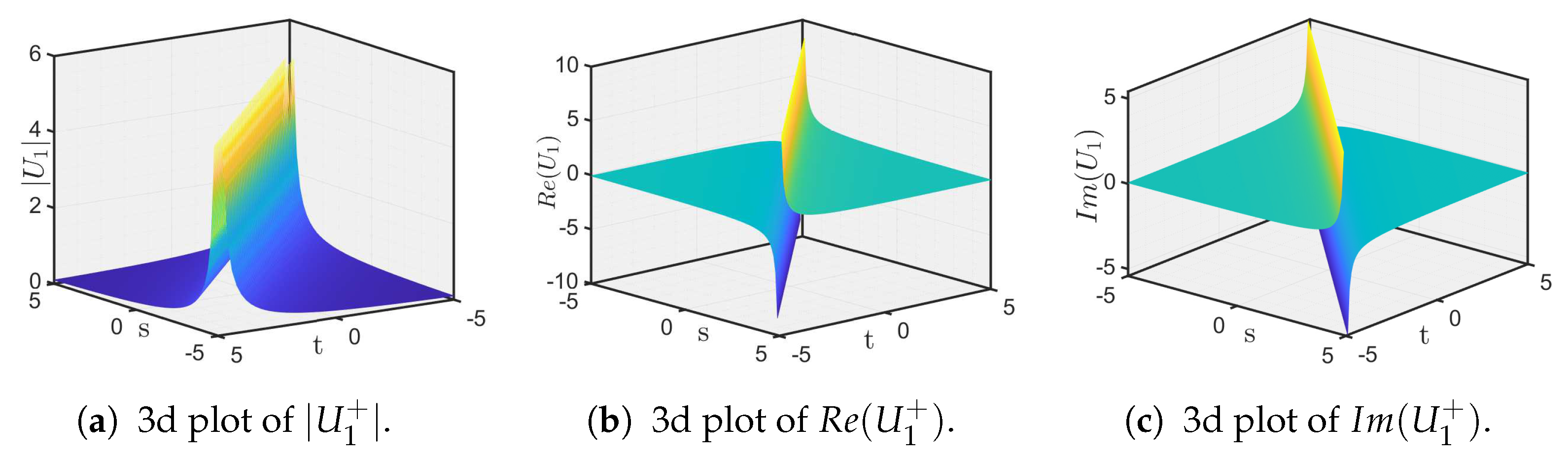
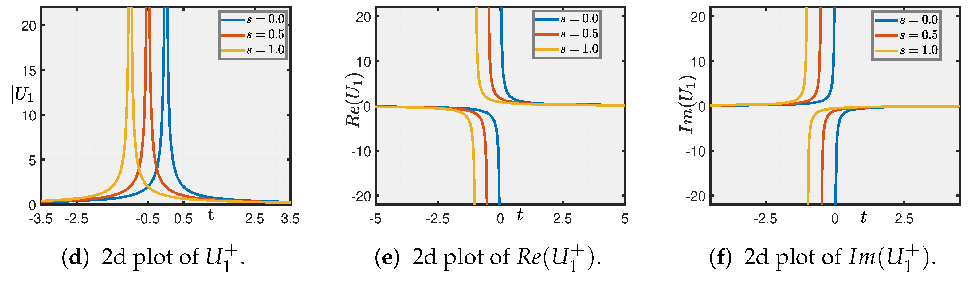
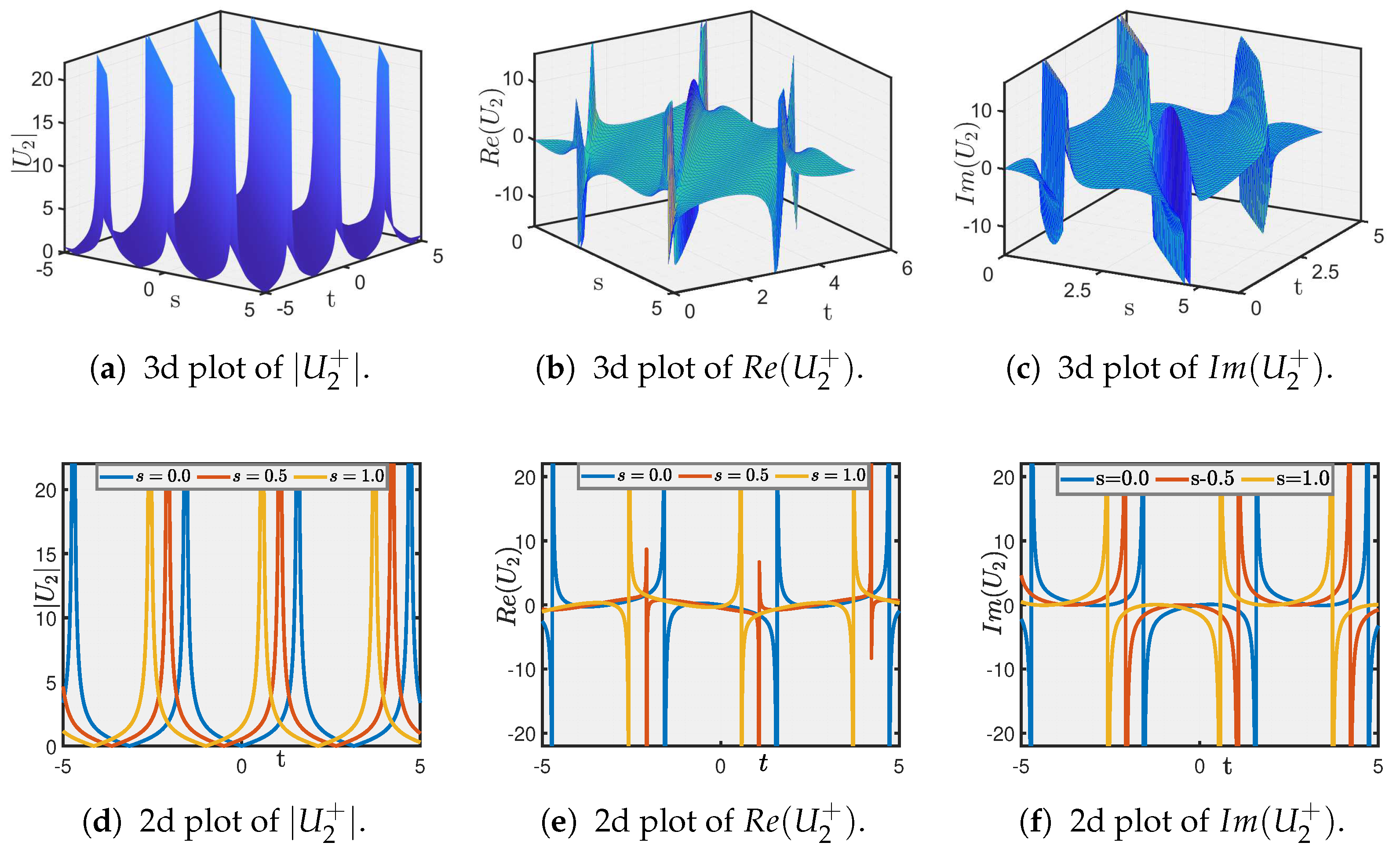
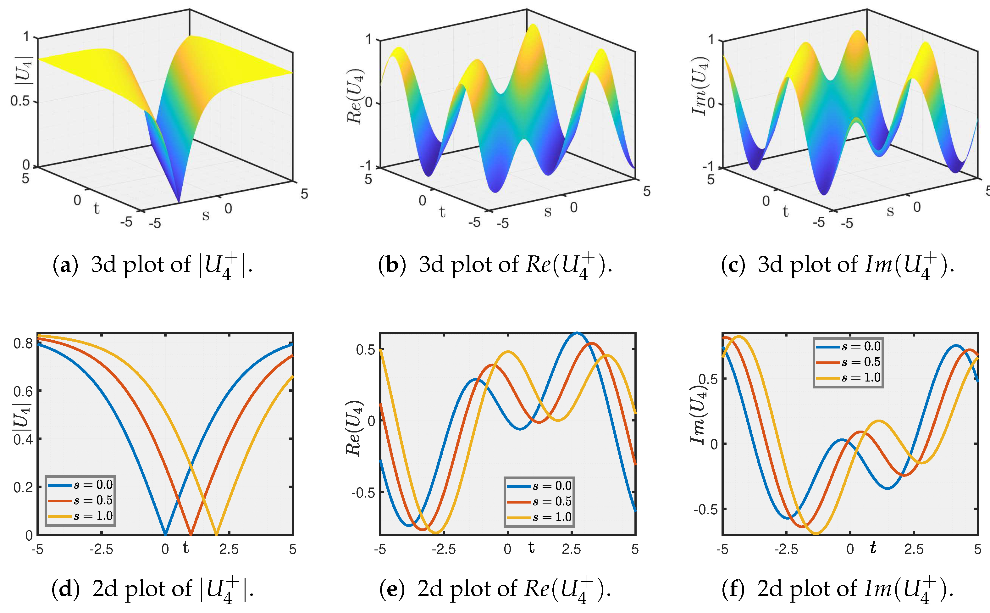
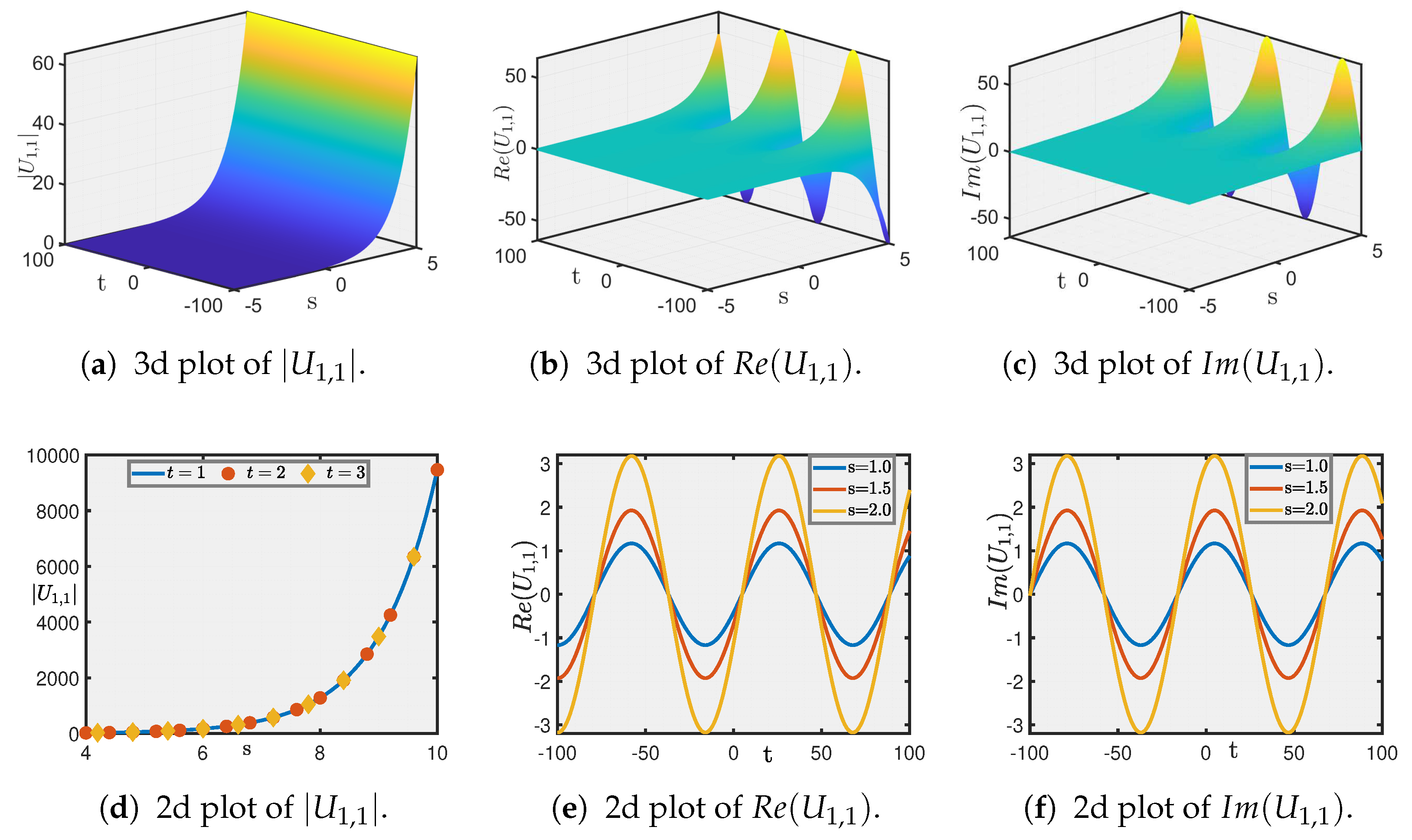
5. Graphical Illustration and Discussion

In this section, we discuss the graphical illustrations and their significance for option pricing.

• In Figure 1, we present the solution $U_1^{+}$ from Equation (40) using the parameter set $p=1,k=1.5,r=0,j=0,\rho =1,\mu =-0.5,\delta =-1$. This solution describes a bright soliton, with its absolute value shown in Figure 1a and its real and imaginary components depicted in Figure 1b,c.
  

  Figure 1. Traveling wave solution $U_1^{+}$ of Equation (40) for $p=1,k=1.5,r=0,j=0,\rho =1,\mu =-0.5$, and $\delta =-1$.
• Figure 2 illustrates the solution $U_2^{+}$ from Equation (41) for the parameter set $p=0.34$, $k=0.67,r=0,j=0,\rho =1,\mu =-1,\delta =-1$. This solution captures the family of singular solitons, with its absolute value presented in Figure 2a and its real and imaginary components in Figure 2b,c.
  

  Figure 2. Traveling wave solution $U_2^{+}$ of Equation (41) for $p=0.34,k=0.67,r=0,j=0,\rho =1$, $\mu =-1$, and $\delta =-1$.
• Figure 3 displays the solution $U_4^{+}$ from Equation (43) using $p=0.98,k=1.35,r=0,$$j=0,\rho =1,\mu =-1,\delta =-1$, yielding a dark soliton. Its absolute value is illustrated in Figure 3a, while its real and imaginary components are shown in Figure 3b,c.
  

  Figure 3. Traveling wave solution $U_4^{+}$ of Equation (43) for $p=0.98,k=1.35,r=0,j=0,\rho =1$, $\mu =-1$, and $\delta =-1$.
• Finally, Figure 4 presents the solution $U_{1,1}$ of Equation (31) using $p=0.97,k=0.23$, $r=0,j=0,\rho =1,\mu =-1,\delta =-1$, yielding a multi-lump soliton, with its absolute value in Figure 4a and its real and imaginary profiles in Figure 4b,c.
  

  Figure 4. Traveling wave solution $U_{1,1}$ of Equation (31) for $p=0.97,k=0.23,r=0,j=0,\rho =1$, $\mu =-1$, and $\delta =-1$.

These soliton structures have direct implications in option pricing, as they reveal the dynamics of option price movements [29,30] and help in understanding phenomena such as sharp price jumps, critical points, and multi-modal fluctuations [31]. Such illustrations and their characteristics can aid in the design of robust pricing and risk management strategies [32,33,34,35].

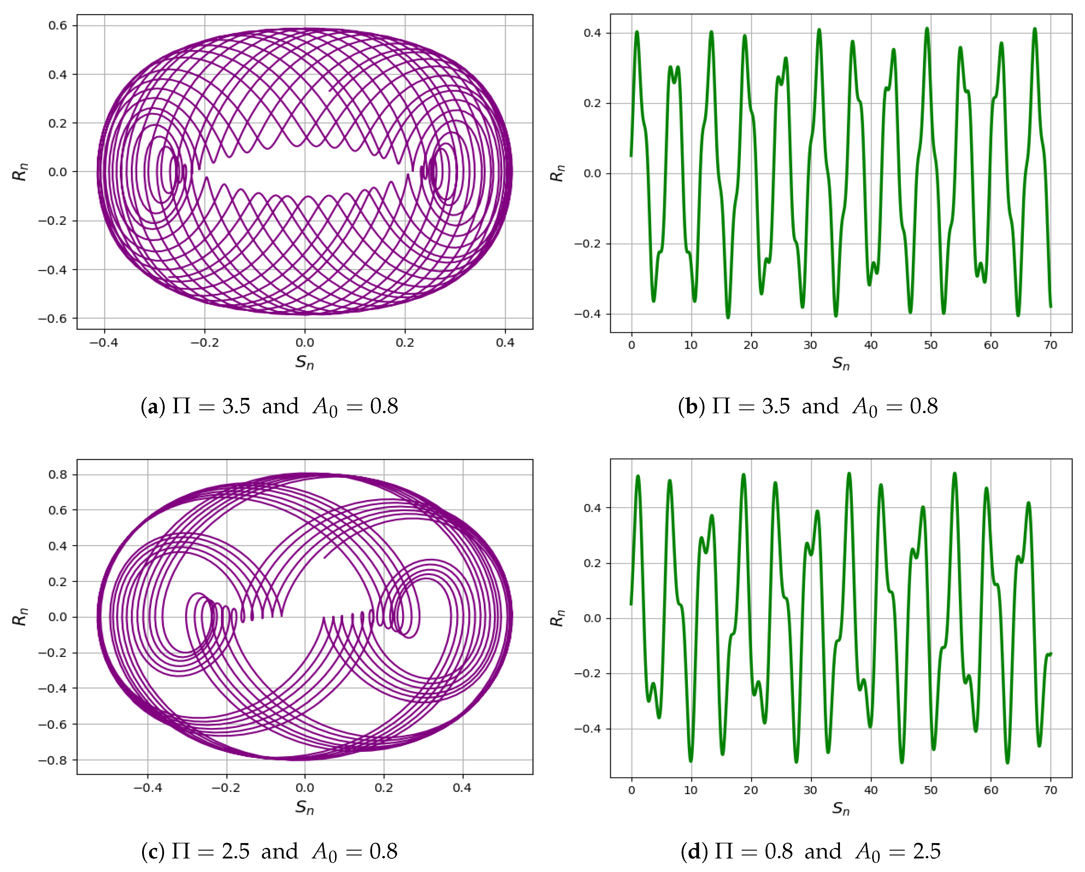
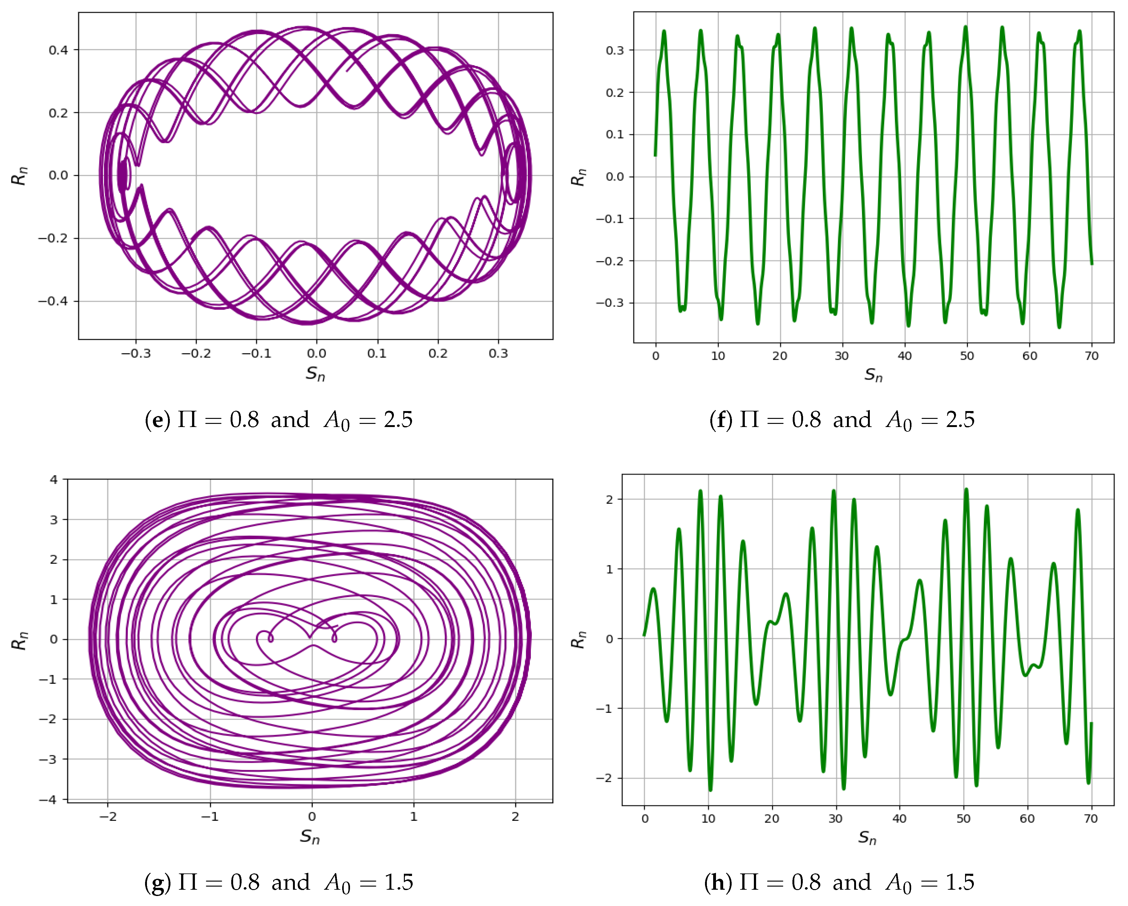
6. Quasi-Periodic Phenomena

The two-dimensional dynamical system represented by Equation (28) can be reformulated as follows [36]:

$$\left\{\begin{array}{c}\begin{array}{cc}\hfill S^{\prime }& =R,\hfill \\ \hfill R^{\prime }& =-{\displaystyle \frac{N{S}^3}{M}}-{\displaystyle \frac{WS}{M}},M\ne 0,\hfill \\ \hfill M& =\mu p^2,N=2\delta ,W=(2j-\mu r^2).\hfill \end{array}\hfill \end{array}\right.$$

(45)

In this step, a small perturbation term is introduced to system (45) as follows:

$$\left\{\begin{array}{c}\begin{array}{cc}\hfill S^{\prime }& =R,\hfill \\ \hfill R^{\prime }& =-{\displaystyle \frac{N{S}^3}{M}}-{\displaystyle \frac{WS}{M}}+A_{0}Cos(\Pi \zeta ),M\ne 0.\hfill \end{array}\hfill \end{array}\right.$$

(46)

$A_0$ and $\Pi$ denote the amplitude and frequency of system (46), respectively. By assigning the parameters $A_0$ and $\omega$, the two-dimensional and time analysis phase portraits of the system (46) are illustrated in Figure 5a–h.

Figure 5. The quasi-periodic behavior of the system (46) under the conditions $S=0.98$, $M=1.34$, and $W-2.34$ is illustrated through two-dimensional phase portraits and time analysis.

6.1. 2D Phase Portrait and Time Analysis

We consider the conditions $N=0.98$, $M=1.34$, and $W-2.34$. The linear combination $A_0^2+\Pi >0$ demonstrates the quasi-periodic behavior of the system, as observed with varying values of $A_0$ and $\Pi$. A comprehensive understanding of intricate behaviors that connect chaotic and periodic dynamics necessitates an in-depth investigation of quasi-periodic patterns present within dynamical systems [34]. Phase portraits shown in Figure 5a–h.These patterns hold significant utility for forecasting and management across a diverse array of fields, as they frequently manifest in real-world phenomena [35,37], including biological rhythms and climate cycles [38,39]. Furthermore, they provide insights into stability analysis and can serve as benchmarks for numerical simulations, thereby fostering interdisciplinary collaboration and innovation [40,41,42].

6.2. Lyapunov Exponent

The Lyapunov exponent constitutes a pivotal metric for assessing system dynamics, particularly within the realms of chaotic and dynamic systems [43,44]. It quantifies the rate at which adjacent trajectories diverge from each other; a positive Lyapunov exponent signifies chaotic behavior, whereas a negative exponent reflects stability [45,46]. This property is vital for the identification of chaotic phenomena and the investigation of the stability associated with equilibrium points or periodic orbits [47,48]. Moreover, the Lyapunov exponent serves as a determinant of a system’s predictability; positive values indicate a sensitive dependence on initial conditions, culminating in unpredictable long-term behavior [49,50]. Its relevance across diverse fields, including engineering, economics [50,51], and meteorology [52,53], underscores the significance of understanding complex systems [54,55]. We calculate the Lyapunov exponent using $S=0.05$, $M=0.5$, $W=0.2$, $A_0=0.8$, and $W=3.5$ with the initial condition $(0.03,0.04)$. The maximal Lyapunov exponent has been determined to be 0.00110, signifying that one of the Lyapunov exponent values is indeed positive [56], thereby corroborating the quasi-periodic dynamics, as illustrated in Figure 6.

Figure 6. Confirm the quasi-periodic behavior of system (46) under the conditions $S>0$, $M>0$, and $W>0$ using the Lyapunov exponent.

6.3. Bifurcation Diagram

A bifurcation diagram visually represents how the qualitative behavior of a system changes as a parameter varies. It is widely applied in nonlinear dynamics to detect transitions between steady states, periodic orbits, and chaos. This tool helps identify critical thresholds and understand system sensitivity with respect to parameter changes. We consider the conditions $N=0.98$, $M=1.34$, and $W=2.34$. The linear combination $A_0^2+\Pi >0$ demonstrates quasi-periodic behavior, as observed in the bifurcation diagram of the system with varying values of $A_0$ and $\Pi$ under two initial conditions, as shown in Figure 7. In the domain $p\in [0,0.3]$, chaotic behavior is observed, while in $p\in [0.31,3]$, the system exhibits quasi-periodic behavior, as shown in Figure 7.

Figure 7. Confirm of the quasi-periodic behavior of system (46) under the conditions $N=0.98$, $M=1.34$, and $W=2.34$, illustrated using the bifurcation diagram. The trajectories starting from initial conditions (0.45, 0.01, 0.05) are shown in red dots, and (0.75, 0.01, 0.05) in cyan dots.

6.4. Multistability

Multistability refers to the coexistence of multiple stable states under the same set of parameters. It appears in various fields such as neuroscience, optics, and ecology, where systems can settle into different behaviors. The advantage lies in offering flexibility and robustness, allowing systems to switch between modes under perturbations. The linear combination $A_0^2+\Pi >0$ demonstrates quasi-periodic behavior, as observed in the bifurcation diagram of the system with varying values of $A_0$ and $\Pi$ under two initial conditions, as shown in Figure 8.

Figure 8. Confirmation of the quasi-periodic behavior of system (46) under the conditions $N=0.98$, $M=1.34$, and $W=2.34$, using multistability analysis.

7. Conclusions

In this paper, we investigate the IOPM, a nonlinear, adaptive-wave approach that serves as an alternative to the classical Black–Scholes option pricing model. By embedding a controlled Brownian motion within a nonlinear Schrödinger framework, the IOPM treats option pricing as a wave function. This approach aims to more accurately reflect real market dynamics by leveraging concepts from mathematics and topology, with the potential to enhance risk management and optimize portfolio strategies. We work on IOPM using following aspects:

• Firstly, we focus on the complex IOPM by applying Lie symmetry analysis. We identify the Lie symmetries of the model and derive the associated symmetry groups, which is pivotal for obtaining exact solutions. This approach provides a structured framework for simplifying the governing equations, making it feasible to gain deeper insights into the dynamics and solution behavior of the model.
• Secondly, we investigate soliton solutions of the IOPM using the unified solver method (USM) and the $({\displaystyle \frac{1}{\varphi \left(\zeta \right)}},{\displaystyle \frac{{\varphi }^{\prime }\left(\zeta \right)}{\varphi \left(\zeta \right)}})$ method. Through these approaches, we obtain a range of wave solutions and present an in-depth qualitative and quantitative investigation of the results. The accompanying 3D and 2D graphical illustrations significantly advance the understanding of the option pricing dynamics, providing a more comprehensive view of the solution landscape.
• These combined analytical and computational techniques offer a significant improvement in both the precision and efficiency of option pricing, making it possible to capture complex market dynamics with higher reliability. The visualizations further deepen our understanding by clearly depicting the interactions and behavior of the solution profiles, facilitating better risk assessment and more robust portfolio optimization.
• Finally, we investigate the quasi-periodic behavior of the two-dimensional dynamical system and its perturbed form using Python-based simulations. By analyzing a range of frequencies and amplitudes, We confirm the presence of quasi-periodic dynamics through the computation of the Lyapunov exponent, bifurcation diagram, and multistability analysis. This approach not only deepens the understanding of the complex dynamics within the IOPM but also contributes to the advancement of financial mathematics by introducing new insights into solution behavior and presenting a robust, comprehensive framework for tackling intricate option pricing problems.

Future Scope: In future studies, we intend to explore conservation laws, develop and implement advanced numerical schemes, investigate lump and multi-soliton solutions, and apply neural network techniques to further deepen the analytical and computational understanding of the IOPM. These extensions will not only enrich the theoretical framework but also broaden its practical applications in financial modeling.

References

1. Han, T.; Rezazadeh, H.; Rahman, M.U. High-order solitary waves, fission, hybrid waves and interaction solutions in the nonlinear dissipative (2 + 1)-dimensional Zabolotskaya-Khokhlov model. Phys. Scr. 2024, 99, 115212. [Google Scholar] [CrossRef]
2. Qin, X.; Yang, W.; Zhang, Z.; Wangari, V.W. Simulation and design of T-shaped barrier tops including periodic split ring resonator arrays for increased noise reduction. Appl. Acoust. 2025, 236, 110751. [Google Scholar] [CrossRef]
3. AL-Essa, L.A.; Rahman, M. Analysis of Lie symmetry, bifurcations with phase portraits, sensitivity and diverse W—M-shape soliton solutions for the (2 + 1)-dimensional evolution equation. Phys. Lett. A 2024, 525, 129928. [Google Scholar] [CrossRef]
4. Yang, H.; Zhang, X.; Hong, Y. Classification, production, and carbon stock of harvested wood products in China from 1961 to 2012. BioResources 2014, 9, 4311–4322. [Google Scholar] [CrossRef]
5. Leung, A.W. Systems of Nonlinear Partial Differential Equations: Applications to Biology and Engineering; Springer Science & Business Media: Berlin/Heidelberg, Germany, 2013; Volume 49. [Google Scholar]
6. Kopçasız, B.; Nur Kaya Sağlam, F. Exploration of Soliton Solutions for the Kaup–Newell Model Using Two Integration Schemes in Mathematical Physics. Math. Methods Appl. Sci. 2025, 48, 6477–6487. [Google Scholar] [CrossRef]
7. Ansari, A.R.; Jhangeer, A.; Imran, M.; Talafha, A.M. Exploring the dynamics of multiplicative noise on the fractional stochastic Fokas-Lenells equation. Partial. Differ. Equ. Appl. Math. 2025, 14, 101232. [Google Scholar] [CrossRef]
8. San, S.; Beenish; Alshammari, F.S. Analytical and Dynamical Study of Solitary Waves in a Fractional Magneto-Electro-Elastic System. Fractal Fract. 2025, 9, 309. [Google Scholar] [CrossRef]
9. Chen, Q.; Baskonus, H.M.; Gao, W.; Ilhan, E. Soliton theory and modulation instability analysis: The Ivancevic option pricing model in economy. Alex. Eng. J. 2022, 61, 7843–7851. [Google Scholar] [CrossRef]
10. Ali, K.K.; Tarla, S.; Ali, M.R.; Yusuf, A.; Yilmazer, R. Physical wave propagation and dynamics of the Ivancevic option pricing model. Results Phys. 2023, 52, 106751. [Google Scholar] [CrossRef]
11. Saglam Ozkan, Y.; Yasar, E. Prolific new M-fractional soliton behaviors to the Schrödinger type Ivancevic option pricing model by two efficient techniques. Comput. Methods Differ. Equ. 2024, 12, 207–225. [Google Scholar]
12. Olver, P.J. Applications of Lie Groups to Differential Equations; Springer Science & Business Media: Berlin/Heidelberg, Germany, 1993; Volume 107. [Google Scholar]
13. Bluman, G.W. Applications of Symmetry Methods to Partial Differential Equations; Springer: Berlin/Heidelberg, Germany, 2010. [Google Scholar]
14. Li, J.; Zhu, X.; Feng, C.; Wen, M.; Zhang, Y. A simple and efficient three-dimensional spring element model for pore seepage problems. Eng. Anal. Bound. Elem. 2025, 176, 106225. [Google Scholar] [CrossRef]
15. Liu, K.; Feng, M.; Zhao, W.; Sun, J.; Dong, W.; Wang, Y.; Mian, A. Pixel-Level Noise Mining for Weakly Supervised Salient Object Detection. IEEE Trans. Neural Netw. Learn. Syst. 2025. [Google Scholar] [CrossRef]
16. Wu, Y.; Guo, Y.; Toyoda, M. Policy iteration approach to the infinite horizon average optimal control of probabilistic Boolean networks. IEEE Trans. Neural Netw. Learn. Syst. 2020, 32, 2910–2924. [Google Scholar] [CrossRef]
17. Guo, Y.; Zhou, R.; Wu, Y.; Gui, W.; Yang, C. Stability and set stability in distribution of probabilistic Boolean networks. IEEE Trans. Autom. Control 2018, 64, 736–742. [Google Scholar] [CrossRef]
18. Wu, Y.; Sun, X.M.; Zhao, X.; Shen, T. Optimal control of Boolean control networks with average cost: A policy iteration approach. Automatica 2019, 100, 378–387. [Google Scholar] [CrossRef]
19. Sağlam, F.N.K.; Kopçasız, B.; Tariq, K.U. Optical Solitons and Dynamical Structures for the Zig-zag Optical Lattices in Quantum Physics. Int. J. Theor. Phys. 2025, 64, 40. [Google Scholar] [CrossRef]
20. Jhangeer, A.; Ansari, A.R.; Imran, M.; Riaz, M.B. Lie symmetry analysis, and traveling wave patterns arising the model of transmission lines. AIMS Math. 2024, 9, 18013–18033. [Google Scholar] [CrossRef]
21. Samreen, M. Exploring quasi-periodic behavior, bifurcation, and traveling wave solutions in the double-chain DNA model. Chaos Solitons Fractals 2025, 192, 116052. [Google Scholar]
22. Beenish; Samreen, M.; Alshammari, F.S. Exploring Solitary Wave Solutions of the Generalized Integrable Kadomtsev–Petviashvili Equation via Lie Symmetry and Hirota’s Bilinear Method. Symmetry 2025, 17, 710. [Google Scholar] [CrossRef]
23. Chou, D.; Boulaaras, S.M.; Rehman, H.U.; Iqbal, I.; Akram, A.; Ullah, N. Additional investigation of the Biswas–Arshed equation to reveal optical soliton dynamics in birefringent fiber. Opt. Quantum Electron. 2024, 56, 705. [Google Scholar] [CrossRef]
24. Feng, G.; Jiang, W.; Liu, J.; Zhang, Q.; Wu, Q.; Miao, L. A novel green nonaqueous sol-gel process for preparation of partially stabilized zirconia nanopowder. Process. Appl. Ceram. 2017, 11, 220–224. [Google Scholar] [CrossRef]
25. Lin, Y.; Li, X.; Huang, L.; Xie, X.; Luo, T.; Tian, G. Acupuncture combined with Chinese herbal medicine for discogenic low back pain: Protocol for a multicentre, randomised controlled trial. BMJ Open 2024, 14, e088898. [Google Scholar] [CrossRef] [PubMed]
26. Nie, Y.; Ji, C.; Yang, H. The forest ecological footprint distribution of Chinese log imports. For. Policy Econ. 2010, 12, 231–235. [Google Scholar] [CrossRef]
27. Feng, G.; Jiang, F.; Jiang, W.; Liu, J.; Zhang, Q.; Wu, Q.; Miao, L. Novel facile nonaqueous precipitation in-situ synthesis of mullite whisker skeleton porous materials. Ceram. Int. 2018, 44, 22904–22910. [Google Scholar] [CrossRef]
28. Jiang, W.H.; Hu, Z.; Liu, J.M. Study on low-tanperature synthesis of iron-stabilized aluminium titanate via non-hydrolytic sol-gel method. J. Syn. Cryst. 2011, 40, 465–469. [Google Scholar]
29. Fang, Q.; Sun, Q.; Ge, J.; Wang, H.; Qi, J. Multidimensional Engineering of Nanoconfined Catalysis: Frontiers in Carbon-Based Energy Conversion and Utilization. Catalysts 2025, 15, 477. [Google Scholar] [CrossRef]
30. Zhou, Y.; Zeng, J.; Yang, Q.; Zhou, L. Rational construction of a fluorescent sensor for simultaneous detection and imaging of hypochlorous acid and peroxynitrite in living cells, tissues and inflammatory rat models. Spectrochim. Acta Part A Mol. Biomol. Spectrosc. 2022, 282, 121691. [Google Scholar] [CrossRef]
31. Liu, W.; Gao, Z.; Wei, Z.; Zhang, L.; Guo, G.; Mumtaz, S. Compensator-Based Fixed-Time Prescribed Performance Control of Vehicular Platoon With Input Nonlinearities: A Performance Boundary Self-Adjusting Approach. IEEE Trans. Intell. Transp. Syst. 2025. [Google Scholar] [CrossRef]
32. Ni, Z.; Ma, J.; Nazarov, A.A.; Yuan, Z.; Wang, X.; Ao, S.; Qin, J. Improving the weldability and mechanical property of ultrasonic spot welding of Cu sheets through a surface gradient structure. J. Mater. Res. Technol. 2025, 36, 2652–2668. [Google Scholar] [CrossRef]
33. Sha, X.; Si, X.; Zhu, Y.; Wang, S.; Zhao, Y. Automatic three-dimensional reconstruction of transparent objects with multiple optimization strategies under limited constraints. Image Vis. Comput. 2025, 160, 105580. [Google Scholar] [CrossRef]
34. Yu, Z.; Ning, Z.; Chang, W.Y.; Chang, S.J.; Yang, H. Optimal harvest decisions for the management of carbon sequestration forests under price uncertainty and risk preferences. For. Policy Econ. 2023, 151, 102957. [Google Scholar] [CrossRef]
35. Feng, M.; Yan, C.; Wu, Z.; Dong, W.; Wang, Y.; Mian, A. Hyperrectangle embedding for debiased 3D scene graph prediction from RGB sequences. IEEE Trans. Pattern Anal. Mach. Intell. 2025, 47, 6410–6426. [Google Scholar] [CrossRef]
36. He, C.H.; Liu, C. A modified frequency–amplitude formulation for fractal vibration systems. Fractals 2022, 30, 2250046. [Google Scholar] [CrossRef]
37. Wu, Y.Z.; Wang, J.; Hu, Y.H.; Sun, Q.S.; Geng, R.; Ding, L.N. Antimicrobial peptides: Classification, mechanism, and application in plant disease resistance. Probiotics Antimicrob. Proteins 2025, 17, 1432–1446. [Google Scholar] [CrossRef]
38. Zeng, M.; Yang, S.; Meng, L.; Jia, S.; Zhou, L.; Lao, X.; Zhou, Y. Developing a de novo designed broth to rapidly recover lactic acid-injured Escherichia coli to ensure almost no multiplication during repair for precise enumeration. Food Control 2023, 153, 109937. [Google Scholar] [CrossRef]
39. Yang, Q.; Zhou, Y.; Tan, L.; Xie, C.; Luo, K.; Li, X.; Zhou, L. Rationally constructed de novo fluorescent nanosensor for nitric oxide detection and imaging in living cells and inflammatory mice models. Anal. Chem. 2023, 95, 2452–2459. [Google Scholar] [CrossRef] [PubMed]
40. Li, Y.Y.; Zhao, X.W.; Zhang, H.H. Out-of-core solver based DDM for solving large airborne array. Appl. Comput. Electromagn. Soc. J. (ACES) 2016, 31, 509–515. [Google Scholar]
41. Zhang, D.; Li, B.; Wei, Y.; Zhang, H.; Lu, G.; Fan, L.; Xu, J. Investigation of injection and flow characteristics in an electronic injector featuring a novel control valve. Energy Convers. Manag. 2025, 327, 119609. [Google Scholar] [CrossRef]
42. Zhang, H.H.; Fan, Z.H.; Chen, R.S. Marching-on-in-degree solver of time-domain finite element-boundary integral method for transient electromagnetic analysis. IEEE Trans. Antennas Propag. 2013, 62, 319–326. [Google Scholar] [CrossRef]
43. Qiu, S.; Qiu, T.; Yan, H.; Long, Q.; Wu, H.; Li, X.; Zhu, D. Investigation of protonation and deprotonation processes of kaolinite and its effect on the adsorption stability of rare earth elements. Colloids Surf. A Physicochem. Eng. Asp. 2022, 642, 128596. [Google Scholar] [CrossRef]
44. Yan, H.; Liang, T.; Liu, Q.; Qiu, T.; Ai, G. Compound leaching behavior and regularity of ionic rare earth ore. Powder Technol. 2018, 333, 106–114. [Google Scholar] [CrossRef]
45. Yin, X.; Lai, Y.; Zhang, X.; Zhang, T.; Tian, J.; Du, Y.; Gao, J. Targeted sonodynamic therapy platform for holistic integrative Helicobacter pylori therapy. Adv. Sci. 2025, 12, 2408583. [Google Scholar] [CrossRef] [PubMed]
46. Yali, D.O.N.G. High-temperature deformatiason measurement using optical imaging digital image correlation: Status, challenge and future. Chin. J. Aeronaut. 2025, 38, 103472. [Google Scholar]
47. Guan, Y.; Cui, Z.; Zhou, W. Reconstruction in off-axis digital holography based on hybrid clustering and the fractional Fourier transform. Opt. Laser Technol. 2025, 186, 112622. [Google Scholar] [CrossRef]
48. Zhang, H.H.; Chao, J.B.; Wang, Y.W.; Liu, Y.; Xu, Y.X.; Yao, H.; Li, X.H. Electromagnetic–thermal co-design of base station antennas with all-metal EBG structures. IEEE Antennas Wirel. Propag. Lett. 2023, 22, 3008–3012. [Google Scholar] [CrossRef]
49. Zhou, Y.; Bu, L.; Guo, M.; Zhou, C.; Wang, Y.; Chen, L.; Liu, J. Comprehensive genomic characterization of Campylobacter genus reveals some underlying mechanisms for its genomic diversification. PLoS ONE 2013, 8, e70241. [Google Scholar] [CrossRef]
50. Zhang, H.; Fan, Z.; Chen, R. Fast wideband scattering analysis based on Taylor expansion and higher-order hierarchical vector basis functions. IEEE Antennas Wirel. Propag. Lett. 2014, 14, 579–582. [Google Scholar] [CrossRef]
51. Yang, Q.; Zhou, L.; Peng, L.; Yuan, G.; Ding, H.; Tan, L.; Zhou, Y. A smart mitochondria-targeting TP-NIR fluorescent probe for the selective and sensitive sensing of H 2 S in living cells and mice. New J. Chem. 2021, 45, 7315–7320. [Google Scholar] [CrossRef]
52. Li, B.; Zhang, Y.; Li, X.; Eskandari, Z.; He, Q. Bifurcation analysis and complex dynamics of a Kopel triopoly model. J. Comput. Appl. Math. 2023, 426, 115089. [Google Scholar] [CrossRef]
53. Zhu, X.; Xia, P.; He, Q.; Ni, Z.; Ni, L. Ensemble Classifier Design Based on Perturbation Binary Salp Swarm Algorithm for Classification. CMES-Comput. Model. Eng. Sci. 2023, 135, 653. [Google Scholar] [CrossRef]
54. Li, B.; Liang, H.; He, Q. Multiple and generic bifurcation analysis of a discrete Hindmarsh-Rose model. Chaos Solitons Fractals 2021, 146, 110856. [Google Scholar] [CrossRef]
55. Zhang, X.; Yang, X.; He, Q. Multi-scale systemic risk and spillover networks of commodity markets in the bullish and bearish regimes. N. Am. J. Econ. Financ. 2022, 62, 101766. [Google Scholar] [CrossRef]
56. Feng, G.; Xie, W.; Zheng, E.; Jiang, F.; Yang, Q.; Jin, W.; Huang, Y. Nonaqueous precipitation combined with intermolecular polycondensation synthesis of novel HAp porous skeleton material and its Pb2+ ions removal performance. Ceram. Int. 2024, 50, 19757–19768. [Google Scholar] [CrossRef]