FIGD-Net: A Symmetric Dual-Branch Dehazing Network Guided by Frequency Domain Information

Abstract

Image dehazing technology is a crucial component in the fields of intelligent transportation and autonomous driving. However, most existing dehazing algorithms only process images in the spatial domain, failing to fully exploit the rich information in the frequency domain, which leads to residual haze in the images. To address this issue, we propose a novel Frequency-domain Information Guided Symmetric Dual-branch Dehazing Network (FIGD-Net), which utilizes the spatial branch to extract local haze features and the frequency branch to capture the global haze distribution, thereby guiding the feature learning process in the spatial branch. The FIGD-Net mainly consists of three key modules: the Frequency Detail Extraction Module (FDEM), the Dual-Domain Multi-scale Feature Extraction Module (DMFEM), and the Dual-Domain Guidance Module (DGM). First, the FDEM employs the Discrete Cosine Transform (DCT) to convert the spatial domain into the frequency domain. It then selectively extracts high-frequency and low-frequency features based on predefined proportions. The high-frequency features, which contain haze-related information, are correlated with the overall characteristics of the low-frequency features to enhance the representation of haze attributes. Next, the DMFEM utilizes stacked residual blocks and gradient feature flows to capture local detail features. Specifically, frequency-guided weights are applied to adjust the focus of feature channels, thereby improving the module’s ability to capture multi-scale features and distinguish haze features. Finally, the DGM adjusts channel weights guided by frequency information. This smooths out redundant signals and enables cross-branch information exchange, which helps to restore the original image colors. Extensive experiments demonstrate that the proposed FIGD-Net achieves superior dehazing performance on multiple synthetic and real-world datasets.

1. Introduction

Haze is an atmospheric phenomenon that degrades the quality of captured images [1]. Image dehazing aims to remove haze from hazy images to enhance image quality, which is of significant importance in applications such as object detection [2]. For instance, vision-based intelligent driving systems are severely affected under foggy conditions and must effectively remove haze to reconstruct high-quality, haze-free images. The formation of haze in images is typically modeled using the atmospheric scattering model, which can be expressed as follows.

$$I(x,y)=J(x,y)t(x,y)+A(x,y)(1-t(x,y))$$

(1)

where $I(x,y)$ represents the hazy image captured by the camera, $J(x,y)$ denotes the clean image to be restored, $A(x,y)$ is the atmospheric light value, $t(x,y)$ is the transmission map, and $t(x,y)$ is determined by the atmospheric scattering coefficient and the scene depth. In the early stages, dehazing algorithms primarily employed hand-crafted prior-based methods [3,4,5]. These methods leveraged the statistical properties or physical models of images to guide the dehazing process. However, hand-crafted prior-based algorithms rely heavily on prior knowledge, and variations in scenes significantly impacted the dehazing performance of these methods. With the rapid development of deep learning, numerous scholars have utilized Convolutional Neural Networks (CNNs) for image dehazing [6,7,8,9,10,11,12], achieving satisfactory experimental results. Nevertheless, these methods faced challenges such as limited receptive fields and suboptimal overall image restoration quality.

As Transformer models have gained widespread application in the field of computer vision, some scholars have proposed dehazing algorithms based on Transformer models [5,13]. However, while Transformers focus on long-range dependencies, they often introduce unnecessary blurring and retain coarse details during the image reconstruction process [13].

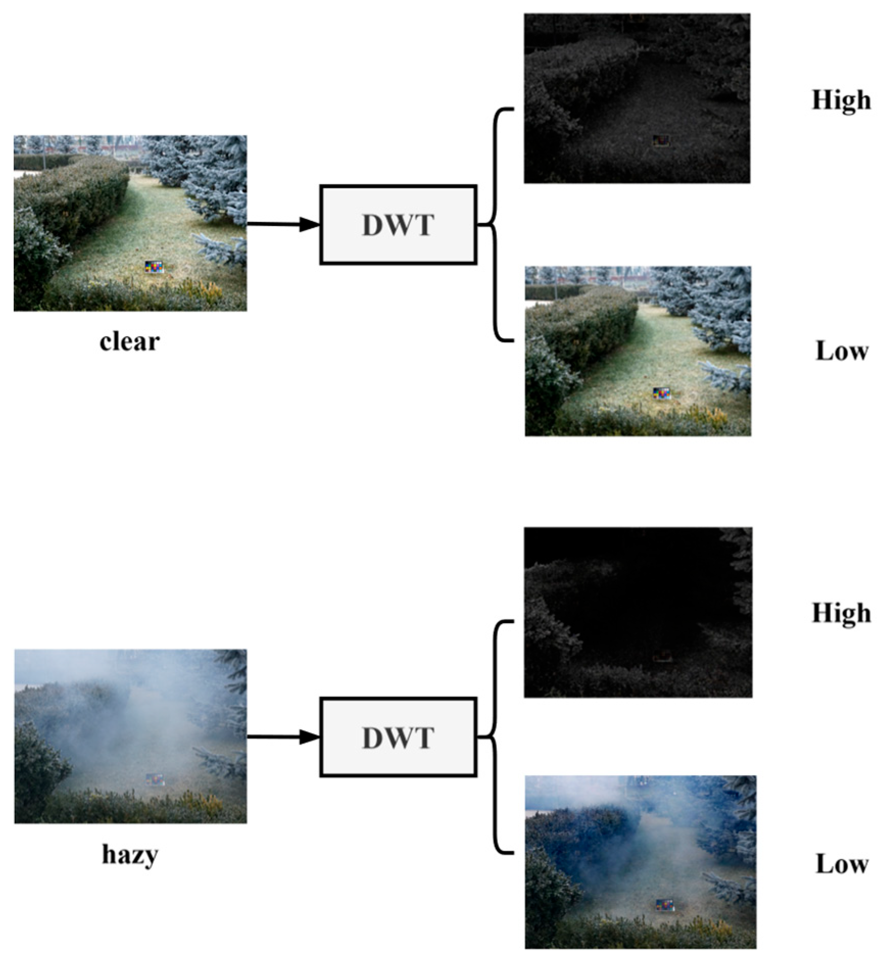
Although the aforementioned image dehazing algorithms have improved dehazing performance, these methods focus on feature recovery in the spatial domain and neglect the impact of haze features in the frequency domain on image restoration. First, haze degradation is a complex nonlinear process, and these nonlinear coupled degradations lead to significant asymmetries in the frequency domain of the image. However, most existing network architectures primarily concentrate on feature learning in the spatial domain [14,15,16], which is insufficient to fully express this nonlinear degradation. To illustrate this more clearly, we used the Discrete Wavelet Transform to separate the high- and low-frequency information in hazy and clear images, as shown in Figure 1. The haze features in hazy images are predominantly present in the high-frequency features and severely interfere with the edge details of the image. Relying solely on spatial domain learning results in mediocre restoration outcomes. Subsequently, traditional CNN operations, limited by their receptive fields, struggle to capture long-range dependencies and non-local texture details. Even when Transformer structures are introduced on top of CNN operations to capture long-range dependencies, this approach still fails to eliminate the impact of haze on the frequency domain.

To address these challenges, we designed a Frequency-Guided Symmetric Dual-Branch Dehazing Network, which includes the Frequency Detail Extraction Module (FDEM), the Multi-scale Frequency-Guided Feature Extraction Module (DMFEM), and the Dual-Domain Guidance Module (DGM). Specifically, first, the FDEM focuses on frequency-domain feature learning. It transforms spatial-domain features into frequency-domain features, extracts both high-frequency and low-frequency features, and uses the global frequency features to guide the feature learning of the CNN module. Second, the DMFEM leverages gradient feature flows to extract local detail features from the image. Finally, the DGM aggregates features from the FDEM and DMFEM to enhance the perception of channel features and frequency-domain features.

Overall, our contributions are as follows.

• We propose a novel dehazing network that utilizes frequency-domain information from the image to guide the spatial-domain feature learning for real-world image dehazing.
• We propose the DMFEM, which enhances the extraction of spatial-domain features by utilizing convolutions with different kernel sizes and gradient feature information, thereby preserving the detail features of the image.
• We introduce the FDEM to fully extract information across different frequencies, focusing particularly on high-frequency features and establishing long-range dependencies in the frequency domain. Additionally, we design the DGM to effectively integrate the frequency information generated by the FDEM with the spatial-domain information from the DMFEM, reducing redundant features and generating guiding weights.
• We conduct experiments on multiple synthetic datasets and real-world scenes, and the results demonstrate the superiority of our model.

2. Related Works

2.1. Image Dehazing

For image dehazing, there are currently two popular approaches. One is to manually analyze the differences between hazy and haze-free images and summarize them as prior knowledge, known as prior-based methods. The other is to directly learn a mapping function based on a dataset, known as data-driven methods.

In the early stages, prior-based methods were the primary approach for image dehazing. For example, the Dark Channel Prior (DCP) algorithm [5] used the dark channel as a tool to estimate the transmission map and reconstructed haze-free images based on the atmospheric scattering model to achieve dehazing. Zhu et al. [6] proposed a method based on color attenuation prior, applying the difference between brightness and saturation to estimate haze concentration. They created a linear regression model related to the scene depth of the hazy image and used supervised learning to train the model parameters, recovering the depth information of the image and then using this depth information to complete the dehazing process. These prior-based methods achieved good dehazing results but only performed well in specific scenarios that met the assumptions.

With the rapid development of deep learning in the field of computer vision, researchers began to focus on data-driven dehazing methods. Early data-driven methods relied on the atmospheric scattering model (ASM). Cai et al. [17] proposed DehazeNet, a trainable end-to-end dehazing model for transmission estimation. However, due to the limitations of the shallow network, the transmission map estimation was inaccurate for scenes with large depth variations. Ren et al. [18] learned the mapping between hazy images and their corresponding transmission maps to remove haze from a single image. Li et al. [19] proposed AOD-Net, which simultaneously estimated the transmission map and the atmospheric light, and then obtained the restored haze-free image using the ASM. However, these ASM-based dehazing models are relatively slow in processing speed [20], and inaccurate estimation of the transmission map and atmospheric light can lead to a decrease in the performance of the restored images.

To avoid the drawbacks of traditional parameter estimation methods, recent research has focused on directly recovering haze-free images from hazy images. Chen et al. [21] integrated smooth expansion techniques into the Gated Context Aggregation Network (GCANet). This method significantly reduced the grid artifacts commonly seen in image processing and designed a gated sub-network that could intelligently fuse features from multiple levels, thereby significantly enhancing the dehazing effect. FFA-Net [22] introduced pixel attention and Channel Attention into the dehazing network to handle different types of information, achieving excellent results on synthetic datasets. SG-Net [23] introduced a semantic guidance (SG) mechanism. By embedding these SG mechanisms into existing dehazing networks, it enhances accuracy with minimal additional time cost. DEA-Net [12] introduced differential convolution into the dehazing network and designed a new convolution operator, significantly enhancing the dehazing effect. A lightweight gated structure was designed by gUNet [24], significantly reducing the network complexity of dehazing algorithms. DehazeFormer [25], based on the Swin Transformer, modified the normalization layer, activation function, and spatial information aggregation scheme, demonstrating superior performance on large-scale remote sensing image dehazing datasets. DADENet [26] enhanced sensitivity to feature information and improved single-image dehazing performance by incorporating Sobel operators and Gaussian blurring into the basic Transformer unit structure.

However, these methods focus on feature learning in the spatial domain and neglect the critical role of the frequency domain in image recovery. Therefore, we utilize the frequency information of images to help achieve end-to-end recovery of hazy images.

2.2. Frequency Information in Image Restoration

Frequency-domain information, as an important feature of images, has been widely used in the field of image restoration. AFENet [27] extracted various frequency band information through convolutions with different kernel sizes and utilizes this information to reconstruct image details, effectively completing the task of image deraining. WF-Diff [28] employed the Discrete Wavelet Transform to separate images into high- and low-frequency features and further uses a diffusion model to reconstruct these frequency features, achieving underwater image restoration. Fourmer [29] leveraged the Fast Fourier Transform to convert spatial information into frequency information and designs a lightweight structure to facilitate frequency-domain feature interaction, demonstrating excellent performance in various image restoration tasks. Wang et al. [30] utilized the Fourier Transform to swap amplitude and phase for image restoration, achieving good results on multiple datasets. FDDN [31] used high-pass filters to divide features into three different frequency bands and processes each band separately, enhancing the ability to extract haze features.

Inspired by these methods, we consider further processing images in the frequency domain to achieve better dehazing effects. As shown in

Table 1. Comparison of frequency extraction methods on the NH-HAZE dataset.

Methods	NH-HAZE		Param (M)	MACs (G)
	PSNR	SSIM
DWT	16.62	0.6107	2.77	10.65
FFT	17.51	0.6042	1.94	5.64
DCT	18.81	0.6611	1.78	4.22

, on the NH-HAZE dataset, we conducted experiments on the frequency extraction methods in the frequency domain branch using common frequency-domain processing methods in the image domain, with experimental settings consistent with Section 4.2, and the results are shown in the table. It can be seen that the Discrete Cosine Transform (DCT) has lower computational complexity compared to the Fast Fourier Transform (FFT) and Discrete Wavelet Transform methods, while maintaining good dehazing performance. This is due to the DCT being a Transform based on cosine functions, whereas the FFT method, since its results are in the form of complex numbers, involves calculations of both the real and imaginary parts, which can make the actual computation slightly more complex than DCT in some cases. The DWT method requires multi-level decomposition of the image, and each level of decomposition involves complex filtering and downsampling operations, greatly increasing the computational cost. Therefore, considering computational overhead and dehazing effect, we choose the DCT method as the frequency extraction method.

3. Methodology

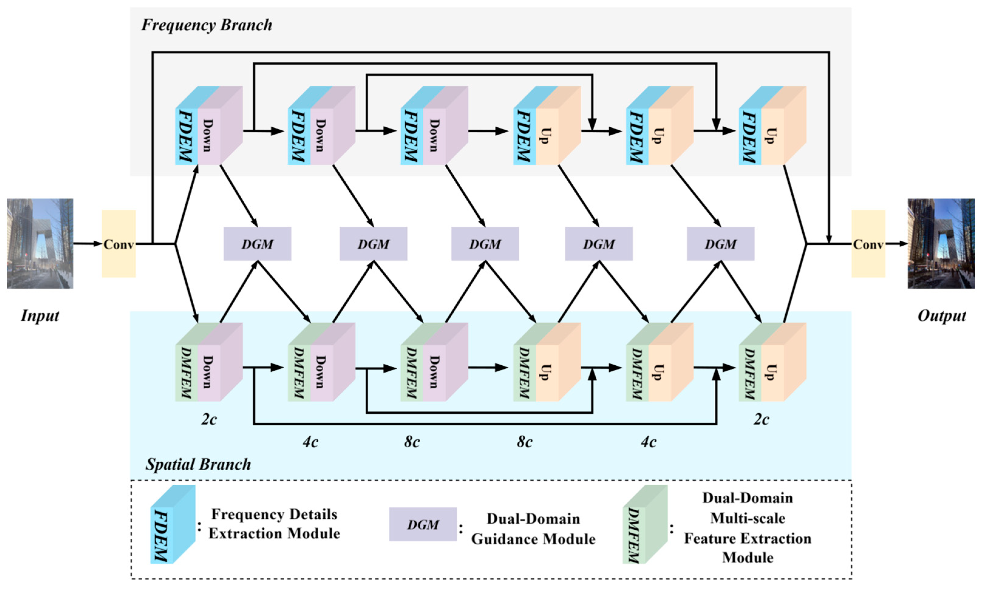
The overall architecture of the FIGD-Net is shown in Figure 2, which mainly consists of three parts: the frequency branch, the spatial branch, and the Dual-Domain Guidance Module (DGM). The overall structure of the FIGD-Net is a dual-branch U-shaped architecture, with three downsampling operations for the encoding process and three upsampling operations for the decoding process in each branch. Both the downsampling and upsampling processes are implemented using strided convolutions.

Given a hazy image, the process begins with adjusting the number of channels using a 3 × 3 convolution. Subsequently, the feature map is fed into the two branches to extract spatial-domain features and frequency-domain features, respectively. During this process, the spatial-domain features and frequency-domain features are sent to the DGM to generate guiding weights, which are then fed back into the spatial branch to guide the learning process. Finally, multiple skip connections are used to preserve detail features and restore the clear image.

3.1. Dual-Domain Multi-Scale Feature Extraction Module

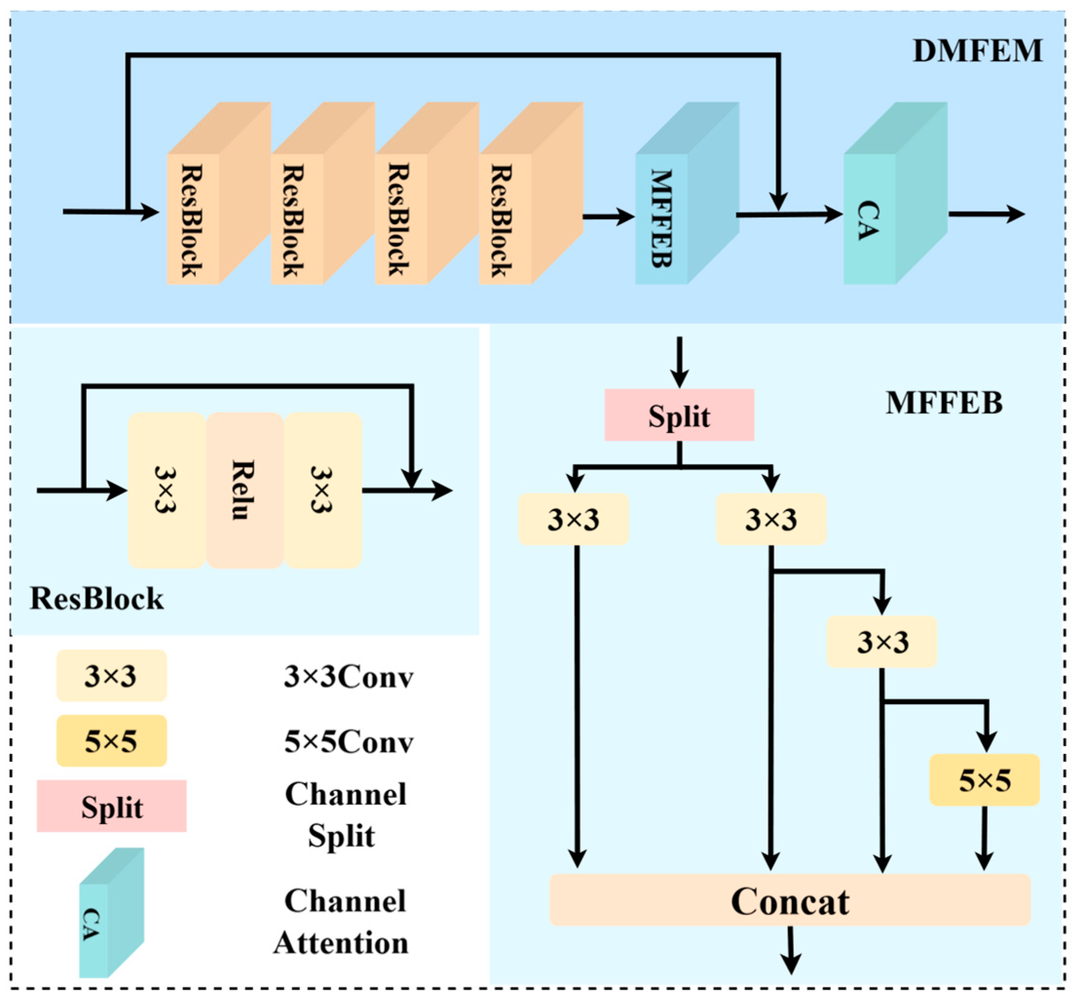
In the task of image dehazing, learning multi-scale features is of great importance [32]. Stacking convolutions with different kernel sizes is a simple way to obtain multi-scale features. However, the introduction of large convolution kernels also brings a significant computational burden. Moreover, since convolution is based on local perception, features extracted solely by convolution can lead to over-extraction of image edges and texture details, resulting in the retention of haze features. Therefore, we designed the Dual-Domain Multi-scale Feature Extraction Module (DMFEM), which consists of Residual Blocks (ResBlocks), Multi-scale Feature Flow Extraction Blocks (MFFEBs), and Channel Attention (CA). The overall structure is shown in Figure 3.

First, by stacking multiple ResBlocks, we obtain the local detail features of the image and gradually integrate these local features. We then multiply the features generated by the ResBlocks with the frequency-guided weights generated by the DGM to adjust the feature information that each feature channel focuses on. This ensures that the subsequent processing pays more attention to haze features. The operation process is as follows:

$$X=f_{res}(f_{res}(f_{res}(f_{res}(F_s))))$$

(2)

$$X_r=X\times F_f$$

(3)

where $F_s$ denotes the feature input from the spatial branch, $f_{res}$ represent the operation of the ResBlock, and $F_f$ indicates the guiding weights generated by the DGM.

Subsequently, the frequency-guided weights are fed into the MFFEB (Multiscale Feature Flow Extraction Block). The MFFEB draws inspiration from the ELAN (Efficient Layer Aggregation Network) architecture in YOLOv7 [33] and improves upon it. Specifically, the input features are split into two main branches, each receiving half of the channels. One of these branches is further divided into two sub-branches, with the channels being split equally again. The last branch uses a 5 × 5 convolution to further obtain multi-scale features, enhance feature representation, and prevent the vanishing gradient phenomenon that occurs with the continuous use of convolution kernels of the same size. This design effectively reduces computational complexity while leveraging both shallow detail information and deep semantic information, establishing long-range dependencies and enhancing the ability to capture multi-scale features and distinguish haze features. The operation process is as follows:

$$X_{m1}^{c/2}=f_{3\times 3}(Split(X_r))$$

(4)

$$X_{m2}^{c/2}=f_{3\times 3}(Split(X_r))$$

(5)

$$X_{m3}^{c/4}=f_{3\times 3}(X_{m2}^{c/2})$$

(6)

$$X_{m4}^{c/4}=f_{5\times 5}(X_{m3}^{c/4})$$

(7)

where $f_{3\times 3}$ and $f_{5\times 5}$ represent 3 × 3 convolution and 5 × 5 convolution. The padding and stride for the 3 × 3 convolution are both 1, and for the 5 × 5 convolution are 2 and 1, respectively. $X_{m1}^{c/2}$, $X_{m2}^{c/2}$, $X_{m3}^{c/4}$, and $X_{m4}^{c/4}$ represent the first, second, third, and fourth branches, respectively.

Finally, the features are integrated through residual connections, and Channel Attention (CA) is applied to focus on the channel features, reducing the redundancy caused by the stacking of convolutions.

3.2. Frequency Details Extraction Module

Current dehazing algorithms perform well on artificially synthesized hazy datasets, as the haze distribution in these datasets is relatively uniform. Each clear image generates multiple hazy images that are perfectly aligned in both time and space. Therefore, even relying solely on CNNs or Transformer networks can achieve satisfactory dehazing results. However, when facing real-world datasets, existing algorithms often fall short due to issues such as misalignment and uneven haze distribution in the data. To address this issue, we design the Frequency Details Extraction Module, which aims to learn haze features in the frequency domain to enhance dehazing performance in real-world scenarios. The structure of this module is shown in Figure 4.

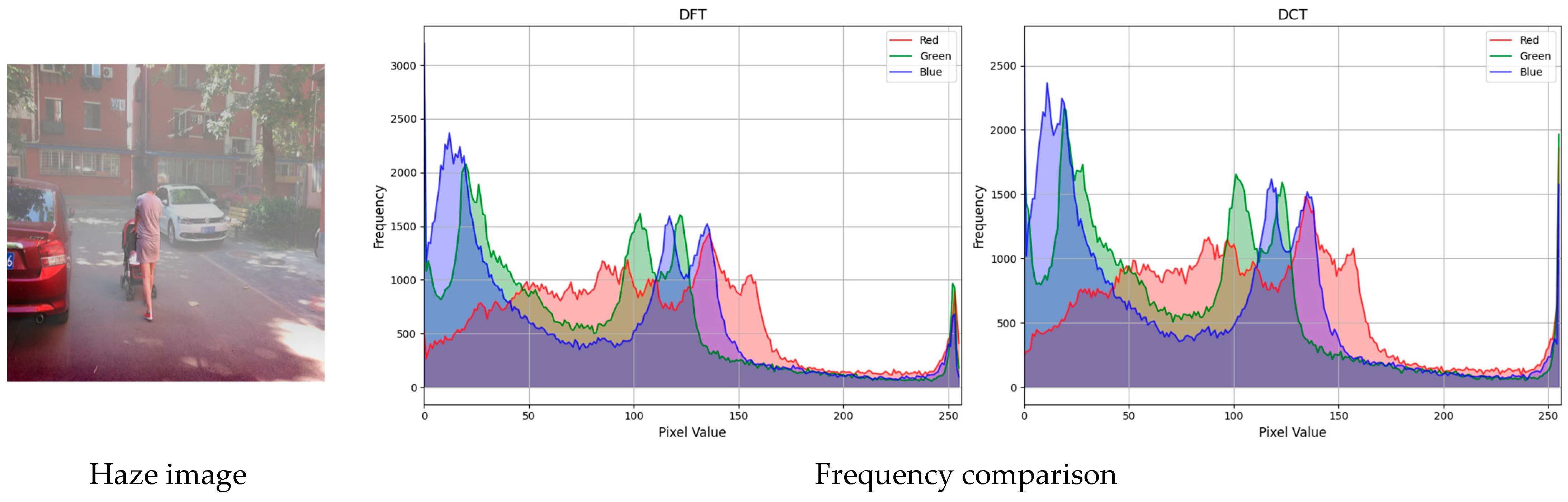
To effectively extract frequency information, ref. [27] employed convolutions with different kernel sizes to capture frequency information, while [34] used a loss function to constrain the frequency information. However, these methods do not guarantee a fully controllable frequency separation. On the other hand, constraining frequency information using a loss function does not explicitly separate frequency components, leading to redundant feature information. Considering these limitations, we adopt the Discrete Cosine Transform (DCT), commonly used in image signal processing, to truly separate frequency components.

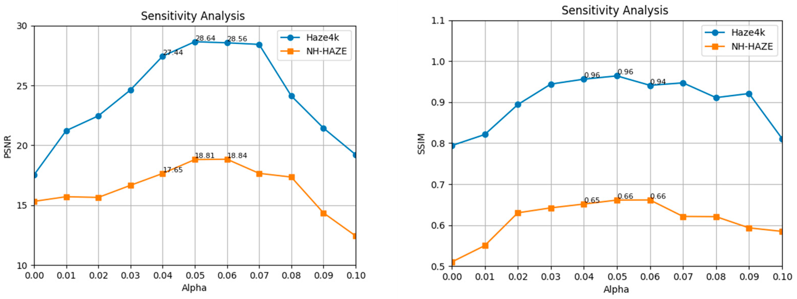
First, we perform the Discrete Cosine Transform on the input features. Leveraging the property that the high-frequency information of the image’s DCT is concentrated in the top-left corner of the feature map, we multiply the generated DCT matrix with a mask matrix to retain both high-frequency and low-frequency information. The high-frequency extraction operation is expressed as follows, and the low-frequency extraction is similar and will not be reiterated here:

$$X_{DCT}=f_{DCT}(X)$$

(8)

$$M_{i,j}=\left\{\begin{array}{l}1, if i<\alpha H and j<\alpha W\\ 0, ortherwise\end{array}\right.$$

(9)

$$X_{high}=X\odot M$$

(10)

where $f_{DCT}$ represent the operations of Discrete Cosine Transform, $M_{i,j}$ denote the generated mask matrix, $H$ and $W$ represent the height and width of the feature map, respectively. $\odot$ represent the element-wise multiplication operation, and $\alpha$ represent the high-frequency information ratio, which is set to 0.05 in this paper.

Next, the Inverse Discrete Cosine Transform (IDCT) is employed to achieve lossless recovery of the original data. The extracted high-frequency and low-frequency information is then fed into a multi-head attention mechanism. By calculating the attention weights between the high-frequency and low-frequency information, the mechanism aggregates the haze-related features from both the low-frequency and high-frequency components. Leveraging the subspace properties of the multi-head attention mechanism, this process captures a more comprehensive set of haze features. The operation can be expressed as follows:

$$Q=DWConv(Conv(X_{high}))$$

(11)

$$\begin{array}{l}KV=DWConv(Conv(X_{low}))\\ K,V=chunk(KV,2)\end{array}$$

(12)

$$\begin{array}{l}scores={\displaystyle \frac{Q{K}^T}{\sqrt{d_k}}}\times temp\\ attn=softmax(scores)\\ out=attn\times V\end{array}$$

(13)

where $Conv$ denotes the 1 × 1 convolution, which is used to map the high-frequency and low-frequency information into the query space; $DWConv$ represents the depthwise separable convolution; $chunk$ splits $KV$ into Key and Value; $temp$ is a learnable parameter used to adjust the degree of attention focus; and soft is used to obtain the final weights.

Finally, the high-frequency feature information is integrated, and a 1 × 1 convolution is used to map the integrated features back to the original number of channels. The operation process can be expressed as follows:

$$out=Conv(out)+X_{high}$$

(14)

3.3. Dual-Domain Guidance Module

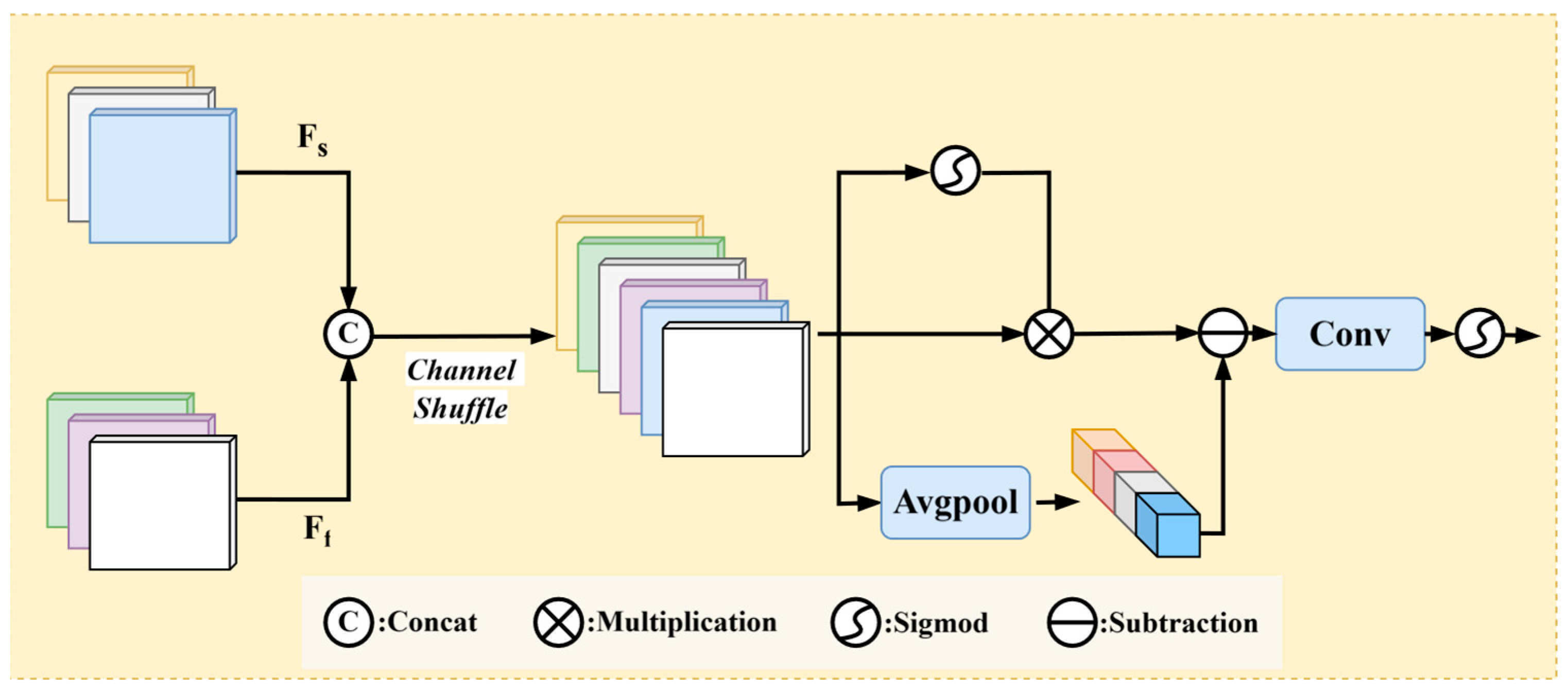
The frequency branch focuses on feature learning in the frequency domain and captures global signal features, while the spatial branch focuses on multi-scale local feature learning. To efficiently transmit the guiding information from the frequency domain to the spatial branch, we designed the Dual-Domain Guidance Module (DGM), the structure of which is shown in Figure 5.

First, the feature maps from the two branches are concatenated and shuffled across channels, allowing for more thorough interaction and fusion of information between different channels. This mechanism helps to break down the isolation of information between channels, enabling the network to more effectively utilize multi-channel features.

Second, the shuffled feature map is passed through an average pooling operation to smooth the features and then subtracted to reduce overall haze interference, preserving the global structure in a balanced manner.

Next, a self-gating mechanism allows the model to dynamically select features that are more helpful for the dehazing task and more important frequency information, thereby enhancing the weights of key features.

Finally, a pointwise convolution adjusts the number of channels, and a sigmoid function generates the guiding weights, which are then fed into the spatial branch to guide its learning process.

The Dual-Domain Guidance Module breaks down the isolation of information between channels, fully interacts different domain features, smooths features through average pooling, reduces overall haze interference, and generates weight information to guide the feature learning in the spatial domain.

3.4. Loss Function

To enhance the feature learning capability in both domains, we propose a dual-domain combined $L_1$ loss function to train the FIGD-Net. However, since PyTorch does not have a direct Discrete Cosine Transform (DCT) function, we implemented it manually. We conducted inference experiments with the Discrete Fourier Transform (DFT) loss function [35] on the Haze4k dataset and analyzed the frequency bias between the inference results of the two to select the most suitable loss function. The results are shown in Figure 6 and

Table 2. Loss Function Comparison Experiment on the NH-HAZE dataset.

Methods	PSNR	Param (M)	MACs (G)
$L_{DCT}$	18.25	1.78	24.44
$L_{DFT}$	18.36	1.78	3.75

.

From Figure 6 and Table 2, it can be seen that there is a certain frequency difference between the inference results of the DCT loss function and the DFT loss function, but it does not affect the image quality. This is due to the fact that DCT is a special case of DFT, and in terms of computational load, the DFT loss function requires much less computation than the manually implemented DFT loss function. Considering the model’s image dehazing capability and model size, we use the DFT as an alternative to the DCT. The definition is as follows:

$$L_1={\displaystyle \frac{1}{e}}\parallel I-Y\parallel ,L_{DCT}={\displaystyle \frac{1}{e}}\parallel F(I)-F(Y)\parallel$$

(15)

where $I$ represents the clear image, $Y$ represents the network-predicted image, $e$ is the total number of elements used for normalization, and $F$ is the Discrete Fourier Transform.

The final loss function is denoted as $L_{loss}=L_1+\lambda L_{DCT}$, with $\lambda$ taking a value of 0.1.

4. Experiments

4.1. Datasets

We conducted experiments on the RESIDE-IN [36], Haze4K [37], and NH-HAZE [38] datasets. For the RESIDE-IN dataset, the ITS (13,990 images) of SOTS was used to train the models, and they were tested on the indoor set (500 images) of SOTS. For the Haze4K dataset, 3000 images from the training set were used for training, and the remaining 1000 images were used for testing. The NH-HAZE dataset is a real-scene dataset with dense and non-uniform haze. The NH-HAZE dataset consists of 55 images in total, including 45 training images, 5 validation images, and 5 test images.

4.2. Training Detail

The experimental hardware platform is a Nvidia GeForce RTX 4090 GPU with 24 GB of video memory, and the software environment includes Windows 11, CUDA 12.4, Python 3.9.19, and PyTorch 2.3.1. The default Adam optimizer is used, with the initial learning rate set to 0.0001. The training is carried out using randomly cropped image patches, and the size of the image patches is gradually scaled from 128 × 128 to the full size during the training process. Meanwhile, the batch size is set to 2.

4.3. Experiments Result

4.3.1. Ablation Experiment

To verify the impact of each module on the overall dehazing performance of the network, we conducted an ablation experiment on the NH-HAZE dataset. We used a single-branch network that only contains the spatial branch and skip connections, with the DMFEM in the spatial branch replaced by ordinary convolution, as the baseline. Then, we added the DMFEM, frequency branch, and DGM sequentially. The experimental configuration has been described in Section 4.2, and the experimental results are shown in

Table 3. Ablation study on the NH-HAZE dataset.

Methods	PSNR	SSIM	Param (M)	MACs (G)
Baseline	12.17	0.4805	0.52	1.66
Baseline + DMFEM (B + D)	14.18	0.5478	1.02	2.54
Baseline + DMFEM + FrequencyBranch (B + D + F)	17.91	0.6415	1.65	3.96
Baseline + DMFEM + FrequencyBranch + DGM (B + D + F + D)	18.81	0.6611	1.78	4.22

,

Table 4. Ablation study on the RESIDE-IN dataset.

Methods	PSNR	SSIM	Param (M)	MACs (G)
Baseline	18.331	0.793	0.52	1.66
Baseline + DMFEM (B + D)	23.655	0.845	1.02	2.54
Baseline + DMFEM + FrequencyBranch (B + D + F)	31.451	0.942	1.65	3.96
Baseline + DMFEM + FrequencyBranch + DGM (B + D + F + D)	33.424	0.964	1.78	4.22

and

Table 5. Ablation study on the Haze4K dataset.

Methods	PSNR	SSIM	Param (M)	MACs (G)
Baseline	16.174	0.821	0.52	1.66
Baseline + DMFEM (B + D)	19.181	0.884	1.02	2.54
Baseline + DMFEM + FrequencyBranch (B + D + F)	26.333	0.945	1.65	3.96
Baseline + DMFEM + FrequencyBranch + DGM (B + D + F + D)	28.645	0.953	1.78	4.22

.

As can be seen from the three tables, each module proposed by us is helpful for the dehazing performance, and the impact of each module on the dehazing performance of the model can be intuitively observed from Figure 7. It can be seen from Figure 7b that after the hazy image is processed by the dehazing model containing only the CNN branch, some light haze is effectively removed. However, when facing thick haze, it is impossible to effectively remove the haze only through the feature analysis in the spatial domain. When the frequency branch is added, as shown in Figure 7c, the thick haze is effectively removed. However, due to the lack of interaction between the spatial and frequency domains, overexposure occurs when restoring the image, resulting in color differences. Finally, the introduction of DGM efficiently combines the two types of features and uses the frequency information to guide the feature learning in the spatial domain, effectively alleviating the overexposure problem, improving the image quality, and achieving the best dehazing performance. In Figure 7, we also provide heatmaps for each module during the dehazing process, allowing for a more intuitive understanding of the focus areas of each module. The heatmaps are implemented using Grad-CAM [39], where the red areas represent high-attention regions, and the yellow areas represent secondary-attention regions.

4.3.2. Sensitivity Analysis

To verify the impact of the value of α in FDEM on the model’s multi-scene dehazing performance, we conducted a sensitivity analysis of the value of α on both synthetic dataset Haze4k and real-world dataset NH-HAZE. The value of α was increased from 0 to 0.1 with an interval of 0.01. Figure 8 shows the effect of different values of α on the experimental results, with the experimental setup consistent with the ablation study.

As can be seen from Figure 8, on both datasets, as the value of α increases, PSNR and SSIM reach their maximum values when α is set to 0.05 and 0.06. This intuitively reflects the importance of high-frequency information for dense fog scenarios. The average maximum values of PSNR and SSIM across both datasets demonstrate that the dehazing effect is optimal when the high-frequency information ratio is set to 0.05.

4.3.3. Results on Synthetic Hazy Images

To illustrate the performance of FIGD-Net on synthetic haze datasets, we compared it with the work of scholars in recent years on two large synthetic haze datasets, RESIDE-IN and Haze4K. The Peak Signal-to-Noise Ratio (PSNR) and Structural Similarity Index Measure (SSIM) were used as evaluation metrics. The higher the PSNR value, the better the image quality, the less distortion, and the smaller the error between the processed image and the clear image. SSIM is used to measure the similarity between two images. The closer the SSIM value is to 1, the more similar the structures of the two images are. Param represents the number of parameters of the model, and MACs represents the computational amount of the model. When calculating the number of parameters and the computational amount, the size of the input tensor is 128 × 128. The experimental results are shown in

Table 6. Quantitative comparison of different methods on the RESIDE-IN dataset.

Methods	Publication	RESIDE-IN		Param (M)	MACs (G)
		PSNR	SSIM
DCP [5]	TPAMI’ 10	16.621	0.818	-	-
AOD-Net [19]	ICCV’ 17	20.513	0.816	0.002	0.115
FFA-Net [22]	AAAI’ 20	29.312	0.914	4.456	287.80
AECR-Net [40]	CVPR’ 21	32.412	0.956	2.611	52.40
OneRestore [41]	ECCV’ 24	32.614	0.951	5.98	-
UCL [42]	TIP’ 24	28.471	0.912	-	-
ICAFormer [43]	2025	30.26	0.96	-	-
Ours	-	33.424	0.964	1.78	4.22

and

Table 7. Quantitative comparison of different methods on the Haze4k dataset.

Methods	Publication	Haze4k		Param (M)	MACs (G)
		PSNR	SSIM
DCP [5]	TPAMI’ 10	14.012	0.760	-	-
AOD-Net [19]	ICCV’ 17	17.152	0.805	0.002	0.115
FFA-Net [22]	AAAI’ 20	25.294	0.896	4.456	287.80
GridDehazeNet [44]	ICCV’ 19	27.566	0.923	0.956	21.49
MSBDN [45]	CVPR’ 20	22.994	0.850	31.35	41.54
Fourmer [29]	ICML’ 23	27.887	0.948	1.29	20.60
DEA-Net [12]	TIP’ 24	28.311	0.952	3.653
Ours	-	28.645	0.953	1.78	4.22

.

From the objective data in Table 6 and Table 7, compared with traditional methods [5,19], end-to-end deep learning methods in recent years have made significant progress. However, the FIGD-Net proposed in this paper achieves better results. On the RESIDE-IN dataset, the PSNR and SSIM of FIGD-Net are 0.81 dB and 0.013 higher than those of the latest method OneRestore [41], which highlights the excellent performance of FIGD-Net on the indoor scene dataset.

In addition, FIGD-Net also performs outstandingly on outdoor synthetic datasets. On the Haze4k dataset, compared with DEA-Net [12], the PSNR and SSIM of FIGD-Net are 0.334 dB and 0.001 higher, respectively, and it also has certain advantages over other methods, reflecting its excellent performance in outdoor scenes. In terms of the number of parameters and computational amount, the method in this paper uses computationally expensive methods such as the attention mechanism in a restrained way. While achieving good dehazing effects, it also maintains a relatively low level of computational amount and the number of parameters.

Figure 9 and Figure 10 analyze the dehazing effect from a subjective perspective. It can be seen from Figure 9 and 10 that FIGD-Net performs well both indoors and outdoors. It leads other methods in the restoration of local textures, which benefits from the full extraction of image details by the spatial branch. Moreover, the color restoration of the image is relatively realistic, while some other methods suffer from the loss of partial detailed textures.

4.3.4. Results on Real-World Images

Synthetic haze datasets typically feature a uniform distribution of haze and a relatively low haze concentration. Under such conditions, most dehazing algorithms are capable of yielding satisfactory dehazing outcomes. In order to provide more robust evidence of the dehazing performance of the algorithm presented in this paper, a comparative experiment was carried out on the real-world haze dataset NH-HAZE. The experimental results are presented in

Table 8. Quantitative comparison of different methods on the NH-HAZE dataset.

Methods	Publication	NH-HAZE		Param (M)	MACs (G)
		PSNR	SSIM
GridDehazeNet [44]	ICCV’ 19	17.23	0.5042	0.956	21.45
SG-Net [23]	ACCV’ 22	18.68	0.6609	3.33	3.34
FFA-Net [22]	AAAI’ 20	18.09	0.5173	4.456	287.8
PSD [46]	CVPR’ 21	10.32	0.5274	6.21	143.91
MSBDN [45]	CVPR’ 20	17.12	0.4539	31.35	41.54
D4 [47]	CVPR’ 22	12.66	0.5072	10.70	2.25
Dehazeformer-T [25]	TIP’ 23	18.73	0.5326	0.68	6.65
SLP [48]	TIP’ 23	15.84	0.5956	-	-
FCTFANet [49]	CVPR’ 25	17.65	0.6514	1.46	37.06
Ours	-	18.81	0.6611	1.78	4.22

.

As can be seen from the data in Table 8, our method achieved the best results in PSNR and SSIM on the NH-HAZE dataset, showing significant advantages over the work of other scholars. This demonstrates that FIGD-Net has the ability to remove more complex hazy images. To make a more intuitive comparison of the dehazing effects, three images were selected for visual comparison, as shown in Figure 11. In the result of D4, there was severe haze residue, and some detailed textures in SLP were not perfectly restored. Moreover, other methods also exhibited some obvious color errors. Our method can remove the patchy fog in real scenes more thoroughly, which benefits from the guidance of frequency-domain information, enabling the model to pay more attention to areas with thick haze. Overall, in terms of subjective evaluation, the methods of other scholars led to color differences and blurring in the NH-HAZE scenes.

In contrast, the images restored by FIGD-Net are closest to the real haze-free images in terms of dehazing and color restoration. Therefore, our method has the best dehazing performance in subjective evaluation.

4.3.5. Histogram Comparison

In order to provide a more intuitive verification of the superiority of the method presented in this paper over the work of other scholars, we incorporated comparison plots of RGB three-channel histograms on both synthetic dataset RESIDE-IN and real-world dataset NH-HAZE. In these plots, the degree to which the trends of the three RGB curves align with that of the clear-image curve serves as an indicator. A closer alignment implies that the image processed by the proposed method bears a greater resemblance to the clear image.

As can be seen from Figure 12 and Figure 13, it becomes evident that the curve distribution of the method presented in this study exhibits a closer resemblance to that of the original image in comparison to other methods. Specifically, other approaches demonstrate substantial deviations in the color distribution of the processed images relative to the original. This finding provides compelling evidence that the method proposed herein is superior to others in terms of the overall restoration of image color, thereby validating its effectiveness and superiority in maintaining the color integrity of the original image during the processing procedure.

4.3.6. Generalization Experiment

To evaluate the robustness of the proposed method beyond the field of dehazing, we expanded our testing scope. We used the low-light dataset LOL [50] as the experimental object, with 485 images for training and 15 images for validation. The objective results are shown in

Table 9. Quantitative comparison of different methods on the LOL dataset.

Methods	Publication	LOL
		PSNR	SSIM
ZeroDCE [51]	CVPR’ 20	15.53	0.67
RetinexNet [50]	BMVC’ 18	12.51	0.65
EnlightenGAN [52]	CVPR’ 20	17.91	0.84
Uformer [53]	CVPR’ 22	20.65	0.87
LLFormer [54]	AAAI’ 23	21.31	0.90
Liu et al. [13]	ACCV’ 24	18.84	0.78
Ours	-	21.52	0.91

, and the subjective experimental results are presented in Figure 14.

The experimental results demonstrate that the method proposed in this paper exhibits excellent performance in low-light images. It has significant advantages over other methods in terms of image color restoration and can more fully restore some detailed textures. Our model has achieved remarkable results in multiple tasks, indicating that this network is suitable for various low-level visual processing tasks.

4.3.7. Real-World Applications

To study the application of the algorithm in real-world scenarios, we introduced the object detection algorithm YOLOv8 [55] to explore the impact of our algorithm on the autonomous driving scenario. First, we trained the YOLOv8n model using the UA-DETRAC [56] dataset and the ExDark [57] dataset, obtaining two sets of optimal training weights. Second, we added haze to the test images of the UA-DETRAC dataset using the atmospheric scattering model and performed low-light enhancement on the test images of the ExDark dataset using the FIGD-Net model trained with the LOL dataset. Then, we used the YOLOv8n model to detect vehicle types in the hazy images, dehazed images, low-light images, and enhanced images. The results are shown in Figure 15 and Figure 16.

As can be discerned from Figure 15 and Figure 16, the FIGD-Net exhibits remarkable performance in haze processing and low-light enhancement. Compared with the original images, it retains details intact, with only minor color deviations. After applying the detection algorithm, the algorithm shows a higher confidence level in detecting nearby vehicle targets in the dehazed and enhanced images. Additionally, it also demonstrates better detection results for distant vehicle targets. This experiment verifies that the FIGD-Net holds great potential in practical applications such as autonomous driving and intelligent transportation.

5. Conclusions

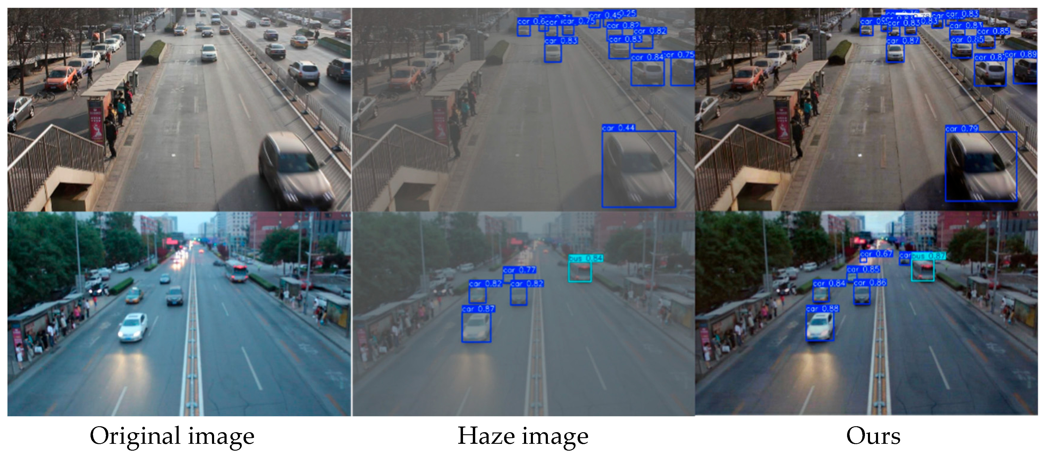
In this paper, we propose a symmetric dual-branch dehazing network guided by frequency-domain information. The proposed model mainly consists of three key modules: the Frequency Detail Extraction Module (FDEM), the Dual-Domain Multi-Scale Feature Extraction Module (DMFEM), and the Dual-Domain Guidance Module (DGM). The FDEM captures global haze features by learning frequency-domain features independently. The DMFEM extracts detailed image features through compact residual blocks and gradient feature information, and utilizes frequency-guided weights to more efficiently complete image restoration. The DGM acquires information from different feature domains, effectively fuses the information, and generates guidance weights for the spatial branch. Extensive experiments demonstrate that the network achieves optimal dehazing performance on multiple datasets. In addition, we applied the network to downstream tasks, which effectively improves the performance of object detection and provides assistance for the fields of intelligent transportation and autonomous driving. However, under extreme conditions, the use of frequency information may cause color differences in the dehazed images. In the future work, we will further optimize the FIGD-Net to enhance the image color restoration ability and explore the applications of FIGD-Net in other fields.

References

1. Sun, H.; Luo, Z.; Ren, D.; Du, B.; Chang, L.; Wan, J. Unsupervised multi-branch network with high-frequency enhancement for image dehazing. Pattern Recognit. 2024, 156, 110763. [Google Scholar] [CrossRef]
2. Zhao, Y.; Lv, W.; Xu, S.; Wei, J.; Wang, G.; Dang, Q.; Liu, Y.; Chen, J. Detrs beat yolos on real-time object detection. In Proceedings of the IEEE/CVF Conference on Computer Vision and Pattern Recognition, Seattle, WA, USA, 16–22 June 2024; pp. 16965–16974. [Google Scholar]
3. Berman, D.; Avidan, S. Non-local image dehazing. In Proceedings of the IEEE Conference on Computer Vision and Pattern Recognition, Las Vegas, NV, USA, 27–30 June 2016; pp. 1674–1682. [Google Scholar]
4. Fattal, R. Dehazing using color-lines. ACM Trans. Graph. 2014, 34, 13. [Google Scholar] [CrossRef]
5. He, K.; Sun, J.; Tang, X. Single image haze removal using dark channel prior. IEEE Trans. Pattern Anal. Mach. Intell. 2010, 33, 2341–2353. [Google Scholar] [PubMed]
6. Zhu, Q.; Mai, J.; Shao, L. A fast single image haze removal algorithm using color attenuation prior. IEEE Trans. Image Process. 2015, 24, 3522–3533. [Google Scholar]
7. Jia, T.; Li, J.; Zhuo, L.; Zhang, J. Self-guided disentangled representation learning for single image dehazing. Neural Networks 2024, 172, 106107. [Google Scholar] [CrossRef]
8. Tong, L.; Liu, Y.; Li, W.; Chen, L.; Chen, E. Haze-aware attention network for single-image dehazing. Appl. Sci. 2024, 14, 5391. [Google Scholar] [CrossRef]
9. Liu, J.; Wang, S.; Chen, C.; Hou, Q. DFP-Net: An unsupervised dual-branch frequency-domain processing framework for single image dehazing. Eng. Appl. Artif. Intell. 2024, 136, 109012. [Google Scholar] [CrossRef]
10. Wang, S.; Hou, Q.; Li, J.; Liu, J. TSID-Net: A two-stage single image dehazing framework with style transfer and contrastive knowledge transfer. Vis. Comput. 2025, 41, 1921–1938. [Google Scholar] [CrossRef]
11. Zhang, X.; Yang, S.; Zhang, Q.; Yuan, F. Multi-scale recurrent attention gated fusion network for single image dehazing. J. Vis. Commun. Image Represent. 2024, 101, 104171. [Google Scholar] [CrossRef]
12. Chen, Z.; He, Z.; Lu, Z.-M. DEA-Net: Single image dehazing based on detail-enhanced convolution and content-guided attention. IEEE Trans. Image Process. 2024, 33, 1002–1015. [Google Scholar] [CrossRef]
13. Liu, H.; Li, X.; Tan, T. Interaction-Guided Two-Branch Image Dehazing Network. In Proceedings of the Asian Conference on Computer Vision, Hanoi, Vietnam, 8–12 December 2024; pp. 4069–4084. [Google Scholar]
14. Ren, W.; Ma, L.; Zhang, J.; Pan, J.; Cao, X.; Liu, W.; Yang, M.-H. Gated fusion network for single image dehazing. In Proceedings of the IEEE Conference on Computer Vision and Pattern Recognition, Salt Lake City, UT, USA, 18–23 June 2018; pp. 3253–3261. [Google Scholar]
15. Song, Y.; Li, J.; Wang, X.; Chen, X. Single image dehazing using ranking convolutional neural network. IEEE Trans. Multimedia 2017, 20, 1548–1560. [Google Scholar] [CrossRef]
16. Huo, Z.; Zhan, X.; Qiao, Y.; Zhao, S. D3-Dehaze: A divide-and-conquer framework for enhanced single image dehazing. Vis. Comput. 2025, 41, 6133–6148. [Google Scholar] [CrossRef]
17. Cai, B.; Xu, X.; Jia, K.; Qing, C.; Tao, D. Dehazenet: An end-to-end system for single image haze removal. IEEE Trans. Image Process. 2016, 25, 5187–5198. [Google Scholar] [CrossRef]
18. Ren, W.; Liu, S.; Zhang, H.; Pan, J.; Cao, X.; Yang, M.-H. Single image dehazing via multi-scale convolutional neural networks. In Proceedings of the Computer Vision–ECCV 2016: 14th European Conference, Amsterdam, The Netherlands, 11–14 October 2016; pp. 154–169. [Google Scholar]
19. Li, B.; Peng, X.; Wang, Z.; Xu, J.; Feng, D. Aod-net: All-in-one dehazing network. In Proceedings of the IEEE International Conference on Computer Vision, Venice, Italy, 22–29 October 2017; pp. 4770–4778. [Google Scholar]
20. Chen, S.; Liu, S.; Chen, X.; Dan, J.; Wu, B. Improved AODNet for Fast Image Dehazing. In Proceedings of the International Conference on Mobile Networks and Management, Yingtan, China, 27–29 October 2023; pp. 154–165. [Google Scholar]
21. Chen, D.; He, M.; Fan, Q.; Liao, J.; Zhang, L.; Hou, D.; Yuan, L.; Hua, G. Gated context aggregation network for image dehazing and deraining. In Proceedings of the 2019 IEEE Winter Conference on Applications of Computer Vision (WACV), Waikoloa, HI, USA, 7–11 January 2019; pp. 1375–1383. [Google Scholar]
22. Qin, X.; Wang, Z.; Bai, Y.; Xie, X.; Jia, H. FFA-Net: Feature fusion attention network for single image dehazing. In Proceedings of the AAAI Conference on Artificial Intelligence, New York, NY, USA, 7–12 February 2020; pp. 11908–11915. [Google Scholar]
23. Hong, T.; Guo, X.; Zhang, Z.; Ma, J. Sg-net: Semantic guided network for image dehazing. In Proceedings of the Asian Conference on Computer Vision, Macao, China, 4–8 December 2022; pp. 274–289. [Google Scholar]
24. Song, Y.; Zhou, Y.; Qian, H.; Du, X. Rethinking performance gains in image dehazing networks. arXiv 2022, arXiv:2209.11448. [Google Scholar]
25. Song, Y.; He, Z.; Qian, H.; Du, X. Vision transformers for single image dehazing. IEEE Trans. Image Process. 2023, 32, 1927–1941. [Google Scholar] [CrossRef]
26. Wei, X.; Ye, X.; Mei, X.; Wang, J.; Ma, H. Enforcing high frequency enhancement in deep networks for simultaneous depth estimation and dehazing. Appl. Soft Comput. 2024, 163, 111873. [Google Scholar] [CrossRef]
27. Yan, F.; He, Y.; Chen, K.; Cheng, E.; Ma, J. Adaptive Frequency Enhancement Network for Single Image Deraining. In Proceedings of the 2024 IEEE International Conference on Systems, Man, and Cybernetics (SMC), Kuching, Malaysia, 6–10 October 2024; pp. 4534–4541. [Google Scholar]
28. Zhao, C.; Cai, W.; Dong, C.; Hu, C. Wavelet-based fourier information interaction with frequency diffusion adjustment for underwater image restoration. In Proceedings of the IEEE/CVF Conference on Computer Vision and Pattern Recognition, Seattle, WA, USA, 16–22 June 2024; pp. 8281–8291. [Google Scholar]
29. Zhou, M.; Huang, J.; Guo, C.-L.; Li, C. Fourmer: An efficient global modeling paradigm for image restoration. In Proceedings of the International Conference on Machine Learning, Honolulu, HI, USA, 23–29 July 2023; pp. 42589–42601. [Google Scholar]
30. Wang, M.; Liao, L.; Huang, D.; Fan, Z.; Zhuang, J.; Zhang, W. Frequency and content dual stream network for image dehazing. Image Vis. Comput. 2023, 139, 104820. [Google Scholar] [CrossRef]
31. Shen, H.; Wang, C.; Deng, L.; He, L.; Lu, X.; Shao, M.; Meng, D. FDDN: Frequency-guided network for single image dehazing. Neural Comput. Appl. 2023, 35, 18309–18324. [Google Scholar] [CrossRef]
32. Cui, Y.; Knoll, A. Psnet: Towards efficient image restoration with self-attention. IEEE Robot. Autom. Lett. 2023, 8, 5735–5742. [Google Scholar] [CrossRef]
33. Wang, C.-Y.; Bochkovskiy, A.; Liao, H.-Y.M. YOLOv7: Trainable bag-of-freebies sets new state-of-the-art for real-time object detectors. In Proceedings of the IEEE/CVF Conference on Computer Vision and Pattern Recognition, Vancouver, BC, Canada, 17–24 June 2023; pp. 7464–7475. [Google Scholar]
34. Pang, Y.; Li, X.; Jin, X.; Wu, Y.; Liu, J.; Liu, S.; Chen, Z. Fan: Frequency aggregation network for real image super-resolution. In Proceedings of the Computer Vision–ECCV 2020 Workshops, Glasgow, UK, 23–28 August 2020; pp. 468–483. [Google Scholar]
35. Liu, J.; Wu, H.; Xie, Y.; Qu, Y.; Ma, L. Trident dehazing network. In Proceedings of the IEEE/CVF Conference on Computer Vision and Pattern Recognition Workshops, Seattle, WA, USA, 14–19 June 2020; pp. 430–431. [Google Scholar]
36. Li, B.; Ren, W.; Fu, D.; Tao, D.; Feng, D.; Zeng, W.; Wang, Z. Benchmarking single-image dehazing and beyond. IEEE Trans. Image Process. 2018, 28, 492–505. [Google Scholar] [CrossRef]
37. Liu, Y.; Zhu, L.; Pei, S.; Fu, H.; Qin, J.; Zhang, Q.; Wan, L.; Feng, W. From synthetic to real: Image dehazing collaborating with unlabeled real data. In Proceedings of the 29th ACM International Conference on Multimedia, Chengdu, China, 20–24 October 2021; pp. 50–58. [Google Scholar]
38. Ancuti, C.O.; Ancuti, C.; Timofte, R. NH-HAZE: An image dehazing benchmark with non-homogeneous hazy and haze-free images. In Proceedings of the IEEE/CVF Conference on Computer Vision and Pattern Recognition Workshops, Seattle, WA, USA, 14–19 June 2020; pp. 444–445. [Google Scholar]
39. Selvaraju, R.R.; Cogswell, M.; Das, A.; Vedantam, R.; Parikh, D.; Batra, D. Grad-cam: Visual explanations from deep networks via gradient-based localization. In Proceedings of the IEEE International Conference on Computer Vision, Venice, Italy, 22–29 October 2017; pp. 618–626. [Google Scholar]
40. Wu, H.; Qu, Y.; Lin, S.; Zhou, J.; Qiao, R.; Zhang, Z.; Xie, Y.; Ma, L. Contrastive learning for compact single image dehazing. In Proceedings of the IEEE/CVF Conference on Computer Vision and Pattern Recognition, Nashville, TN, USA, 19–25 June 2021; pp. 10551–10560. [Google Scholar]
41. Guo, Y.; Gao, Y.; Lu, Y.; Zhu, H.; Liu, R.W.; He, S. Onerestore: A universal restoration framework for composite degradation. In Proceedings of the European Conference on Computer Vision, Milan, Italy, 29 September–4 October 2024; pp. 255–272. [Google Scholar]
42. Wang, Y.; Yan, X.; Wang, F.L.; Xie, H.; Yang, W.; Zhang, X.-P.; Qin, J.; Wei, M. UCL-Dehaze: Toward real-world image dehazing via unsupervised contrastive learning. IEEE Trans. Image Process. 2024, 33, 1361–1374. [Google Scholar] [CrossRef] [PubMed]
43. Chen, Y.; Yue, T.; An, P.; Hong, H.; Liu, T.; Liu, Y.; Zhou, Y. ICAFormer: An Image Dehazing Transformer Based on Interactive Channel Attention. Sensors 2025, 25, 3750. [Google Scholar] [CrossRef] [PubMed]
44. Liu, X.; Ma, Y.; Shi, Z.; Chen, J. Griddehazenet: Attention-based multi-scale network for image dehazing. In Proceedings of the IEEE/CVF International Conference on Computer Vision, Seoul, Republic of Korea, 27 October–2 November 2019; pp. 7314–7323. [Google Scholar]
45. Dong, H.; Pan, J.; Xiang, L.; Hu, Z.; Zhang, X.; Wang, F.; Yang, M.-H. Multi-scale boosted dehazing network with dense feature fusion. In Proceedings of the IEEE/CVF Conference on Computer Vision and Pattern Recognition, Seattle, WA, USA, 14–19 June 2020; pp. 2157–2167. [Google Scholar]
46. Chen, Z.; Wang, Y.; Yang, Y.; Liu, D. PSD: Principled synthetic-to-real dehazing guided by physical priors. In Proceedings of the IEEE/CVF Conference on Computer Vision and Pattern Recognition, Nashville, TN, USA, 19–25 June 2021; pp. 7180–7189. [Google Scholar]
47. Yang, Y.; Wang, C.; Liu, R.; Zhang, L.; Guo, X.; Tao, D. Self-augmented unpaired image dehazing via density and depth decomposition. In Proceedings of the IEEE/CVF Conference on Computer Vision and Pattern Recognition, New Orleans, LA, USA, 19–20 June 2022; pp. 2037–2046. [Google Scholar]
48. Ling, P.; Chen, H.; Tan, X.; Jin, Y.; Chen, E. Single image dehazing using saturation line prior. IEEE Trans. Image Process. 2023, 32, 3238–3253. [Google Scholar] [CrossRef]
49. Monga, A.; Nehete, H.; Kaushik, P.; Bollu, T.K.R.; Raman, B.; Sharma, G. FCTFANet: A Fused CNN-Transformer Feature Aggregator Network for Image Restoration. In Proceedings of the Computer Vision and Pattern Recognition Conference, Nashville, TN, USA, 16–20 June 2025; pp. 885–894. [Google Scholar]
50. Wei, C.; Wang, W.; Yang, W.; Liu, J. Deep retinex decomposition for low-light enhancement. arXiv 2018, arXiv:1808.04560. [Google Scholar]
51. Guo, C.; Li, C.; Guo, J.; Loy, C.C.; Hou, J.; Kwong, S.; Cong, R. Zero-reference deep curve estimation for low-light image enhancement. In Proceedings of the IEEE/CVF Conference on Computer Vision and Pattern Recognition, Seattle, WA, USA, 14–19 June 2020; pp. 1780–1789. [Google Scholar]
52. Jiang, Y.; Gong, X.; Liu, D.; Cheng, Y.; Fang, C.; Shen, X.; Yang, J.; Zhou, P.; Wang, Z. Enlightengan: Deep light enhancement without paired supervision. IEEE Trans. Image Process. 2021, 30, 2340–2349. [Google Scholar] [CrossRef]
53. Wang, Z.; Cun, X.; Bao, J.; Zhou, W.; Liu, J.; Li, H. Uformer: A general u-shaped transformer for image restoration. In Proceedings of the IEEE/CVF Conference on Computer Vision and Pattern Recognition, New Orleans, LA, USA, 19–20 June 2022; pp. 17683–17693. [Google Scholar]
54. Wang, T.; Zhang, K.; Shen, T.; Luo, W.; Stenger, B.; Lu, T. Ultra-high-definition low-light image enhancement: A benchmark and transformer-based method. In Proceedings of the AAAI conference on artificial intelligence, Washington, DC, USA, 7–14 February 2023; pp. 2654–2662. [Google Scholar]
55. Varghese, R.; Sambath, M. Yolov8: A novel object detection algorithm with enhanced performance and robustness. In Proceedings of the 2024 International Conference on Advances in Data Engineering and Intelligent Computing Systems (ADICS), Chennai, India, 18–19 April 2024; pp. 1–6. [Google Scholar]
56. Wen, L.; Du, D.; Cai, Z.; Lei, Z.; Chang, M.-C.; Qi, H.; Lim, J.; Yang, M.-H.; Lyu, S. UA-DETRAC: A new benchmark and protocol for multi-object detection and tracking. Comput. Vis. Image Underst. 2020, 193, 102907. [Google Scholar] [CrossRef]
57. Loh, Y.P.; Chan, C.S. Getting to know low-light images with the exclusively dark dataset. Comput. Vis. Image Underst. 2019, 178, 30–42. [Google Scholar] [CrossRef]
Figure 1. Discrete Wavelet Transform of images.
Symmetry 17 01122 g001
Figure 2. Overall architecture of the FIGD-Net.
Symmetry 17 01122 g002
Figure 3. Structure of the Dual-Domain Multi-scale Feature Extraction Module.
Symmetry 17 01122 g003
Figure 4. Structure of the Frequency Detail Extraction Module.
Symmetry 17 01122 g004
Figure 5. Structure of the Dual-Domain Guidance Module.
Symmetry 17 01122 g005
Figure 6. Frequency comparison after reasoning by two methods.
Symmetry 17 01122 g006
Figure 7. Ablation study of different modules. The red bounding boxes allow the dehazing results of each algorithm to be observed more clearly.
Symmetry 17 01122 g007
Figure 8. Sensitivity analysis on synthetic dataset Haze4k and real-world dataset NH-HAZE.
Symmetry 17 01122 g008
Figure 9. Subjective comparison of different methods on the RESIDE-IN dataset. The red bounding boxes allow the dehazing results of each algorithm to be observed more clearly.
Symmetry 17 01122 g009
Figure 10. Subjective comparison of different methods on the Haze4k dataset. The red bounding boxes allow the dehazing results of each algorithm to be observed more clearly.
Symmetry 17 01122 g010
Figure 11. Subjective comparison of different methods on the NH-HAZE dataset. The red bounding boxes allow the dehazing results of each algorithm to be observed more clearly.
Symmetry 17 01122 g011
Figure 12. Histogram comparison of different methods on RESIDE-IN dataset.
Symmetry 17 01122 g012
Figure 13. Histogram comparison of different methods on NH-HAZE dataset.
Symmetry 17 01122 g013
Figure 14. Subjective comparison of different methods on the LOL dataset.
Symmetry 17 01122 g014
Figure 15. Application of FIGD-Net in Hazy Weather Object Detection.
Symmetry 17 01122 g015
Figure 16. Application of FIGD-Net in low-light object detection.
Symmetry 17 01122 g016