A General Model Construction and Operating State Determination Method for Harmonic Source Loads

Abstract

The widespread integration of power electronic devices and renewable energy sources into power systems has significantly exacerbated voltage and current waveform distortion issues, where asymmetric loads—including single-phase nonlinear equipment and unbalanced three-phase power electronic installations—serve as critical harmonic sources whose inherent nonlinear and asymmetric characteristics increasingly compromise power quality. To enhance power quality management, this paper proposes a universal harmonic source modeling and operational state identification methodology integrating physical mechanisms with data-driven algorithms. The approach establishes an RL-series equivalent impedance model as its physical foundation, employing singular value decomposition and Z-score criteria to accurately characterize asymmetric load dynamics; subsequently applies Variational Mode Decomposition (VMD) to extract time-frequency features from equivalent impedance parameters while utilizing Density-Based Spatial Clustering (DBSCAN) for the high-precision identification of operational states in asymmetric loads; and ultimately constructs state-specific harmonic source models by partitioning historical datasets into subsets, substantially improving model generalizability. Simulation and experimental validations demonstrate that the synergistic integration of physical impedance modeling and machine learning methods precisely captures dynamic harmonic characteristics of asymmetric loads, significantly enhancing modeling accuracy, dynamic robustness, and engineering practicality to provide an effective assessment framework for power quality issues caused by harmonic source integration in distribution networks.

1. Introduction

With the continuous development and intelligent upgrading of power systems, a large number of power electronic devices and renewable energy generation equipment have been connected to the grid, leading to a rapid increase in the types and quantities of harmonic sources [1]. As a result, the distortion of voltage and current waveforms has become increasingly prominent. Harmonic pollution not only reduces power quality but may also cause a series of issues such as accelerated wear and tear of power equipment and misoperation of relay protection systems, seriously threatening the safety and stable operation of the power system [2,3,4]. Therefore, to formulate scientific and effective measures for preventing and mitigating harmonic pollution, it is imperative to establish accurate and reliable harmonic source load models.

Currently, harmonic source modeling methods can be primarily divided into two categories: mechanism-based modeling and data-driven modeling. Mechanism-based modeling methods analyze the internal working principles of harmonic sources to construct mathematical models that reflect the intrinsic nature of harmonic generation. In [5], the dead time of inverters and the actual switching characteristics of power devices were utilized to model specific harmonic sources. In [6], white noise signals were employed to modulate static arc parameters, successfully simulating the randomness of electric arc furnace operation, and a time-domain mathematical model was derived based on energy conservation. Building upon this, the authors of [7] used chaotic signals generated by an asymmetric nonlinear resistor Chua’s circuit to modulate arc parameters, deriving a precise AC electric arc furnace model. In [8], a mathematical model for medium-frequency harmonic currents on the stator side of a DFIG under typical vector control was constructed. This model reflects the influence of power supply conditions, control parameters, and operating conditions on stator-side harmonic currents, providing methods and a basis for harmonic assessment and mitigation. However, the authors did not discuss the harmonic current characteristics at the grid-side converter and the point of common coupling (PCC). While the aforementioned models exhibit high accuracy, they heavily rely on the internal topology and parameters of the loads. Given the wide variety of harmonic sources and their differing mechanisms, the applicability of such models is relatively limited.

Data-driven modeling methods can be divided into two categories: one involves uncovering the relationships between various characteristic quantities of harmonic sources to solve the mapping relationships between these quantities, while the other focuses on analyzing the intrinsic structure of harmonic data to predict and assess harmonic characteristics. The first approach begins by identifying relevant physical quantities related to the harmonic emission characteristics of harmonic sources (e.g., supply voltage, power, equipment parameters, and natural conditions such as solar irradiance and wind speed in renewable energy systems). These physical quantities are then used as inputs, and machine learning algorithms such as neural networks [9], support vector machines (SVMs) [10], and transfer learning and attention mechanisms [11] are employed to establish a nonlinear mapping relationship between the inputs and harmonic outputs in a black-box manner, revealing hidden correlations [12,13,14,15]. The second approach typically starts from the time-series characteristics of harmonic monitoring data, using clustering algorithms to identify the operational states and harmonic characteristics of harmonic sources [16]. Alternatively, methods such as long short-term memory neural networks [17], autoregressive integrated moving average (ARIMA) models [18], Bayesian Deep Learning [19], and adaptive Kalman filtering [20] are applied to analyze the temporal features of harmonic sources and construct models for harmonic prediction. The modeling target of this method mainly depends on whether the data source is a monitoring point in a distribution system or a monitoring device for a specific harmonic source. In most cases, this approach is used for modeling individual harmonic sources. In summary, data-driven harmonic source models bypass the complex mechanism analysis process and offer simplicity and ease of construction. However, these models lack actual physical significance and interpretability, and their performance heavily depends on data volume, data quality, and computational resources. Additionally, constrained by limited data samples from specific scenarios, current data-driven harmonic source models can only describe partial harmonic emission characteristics under certain operating conditions of harmonic-producing equipment, making it difficult to achieve comprehensive learning and regression across all operational states [21].

To address the above issues, this paper proposes a general model construction and operation state determination method for harmonic source loads based on load equivalent impedance parameters. The method uses an RL-series equivalent impedance model to describe the dynamic characteristics of the load and combines the Variational Mode Decomposition (VMD) and Density-Based Spatial Clustering of Applications with Noise (DBSCAN) algorithms to realize the operation state identification and feature extraction of asymmetric loads. The singular value decomposition method is adopted to solve the equivalent impedance parameters, and the Z-score criterion is used to eliminate outliers, so as to improve the model’s accuracy. This method not only overcomes the defect of low applicability of traditional mechanism modeling but also makes up for the lack of physical meaning of data-driven modeling, providing a reliable theoretical basis and technical support for harmonic governance.

2. General Model of Harmonic Source Load

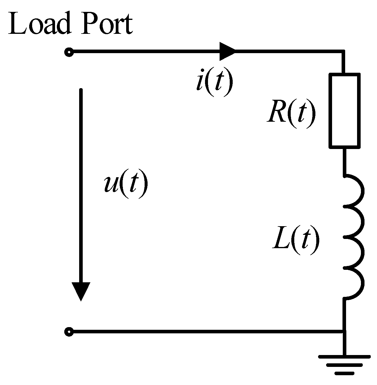
2.1. Basic Principle of Load Equivalent Impedance Parameters

In view of the fact that most harmonic source loads exhibit resistive–inductive characteristics [5], this study selects the widely used RL-series equivalent impedance model to represent the equivalent impedance parameters of the load in the time domain, as shown in Figure 1. In the figure, the voltage and current measurements at the monitoring point are represented by u(t) and i(t); R(t) and L(t) represent the time-varying equivalent impedance parameters of the load, which can accurately capture the dynamic characteristics of the load changing with time.

Based on Thevenin’s theorem and using the voltage and current data measured at the load port monitoring point, the following relationship between the load current and voltage can be derived:

$$u(t)=i(t)R(t)+L(t){\displaystyle \frac{\mathrm{d}i(t)}{\mathrm{d}t}}$$

(1)

Drawing on the concept of infinitesimal analysis, we perform piecewise linearization calculations for time-varying load equivalent impedance parameters. When the variation frequency of load equivalent impedance parameters is substantially lower than the sampling frequency, the parameters can be considered constant between two consecutive sampling points within an infinitesimal time interval [22,23]. Under this premise, the mathematical transformation of Equation (1) enables the construction of differential equations or small-signal models, facilitating parameter solving through least squares or singular value decomposition methods.

It should be particularly noted that in practical engineering applications, a large number of common harmonic source loads exhibit inductance-dominant characteristics [23]. Even for some devices that integrate small-capacity EMI filtering capacitors or other capacitive components, the inductive reactance component still dominates at the power frequency and major low-order harmonic frequencies (e.g., the fifth and seventh harmonics). Furthermore, from the perspective of mathematical structure, RC models are isomorphic to RL models in terms of their mathematical formulations. Therefore, the proposed RL equivalent model in this paper can achieve a unified characterization of both inductive and capacitive behaviors through generalized reactance parameters: when the equivalent inductance parameter L(t) > 0, the model represents inductive load behavior; when L(t) < 0, the negative inductance value corresponds to the equivalent reactance characteristic of a capacitive load.

2.2. Model Parameter Solution

Aiming to address the problem that the least squares method may lead to the distortion of parameter estimation results when the sampling frequency is too low or too high, this paper adopts a more robust parameter solution method, namely the singular value decomposition (SVD) method. This method can determine a unique solution with the minimum norm in the least squares solution when the measurement matrix is ill-conditioned so as to improve the accuracy of parameter identification. Suppose measurement matrix A is an m×n matrix, then matrix A can be decomposed into the following form:

$$A_{m\times n}=U_{m\times m}\left[\begin{array}{c}\begin{array}{cc}\sum & 0\end{array}\\ \begin{array}{cc}0& 0\end{array}\end{array}\right]V_{n\times n}^T$$

(2)

where U and V^T are orthogonal matrices, representing the left singular vectors and right singular vectors of matrix A, respectively; Σ is a diagonal matrix, and its main diagonal elements $\left[{\delta }_1,{\delta }_2,\cdots ,{\delta }_r\right]$ are called the singular values of matrix A, satisfying ${\delta }_1\ge {\delta }_2\ge ...\ge {\delta }_r\ge 0$. r denotes the rank of the matrix, and $r\le min$(m,n).

The generalized inverse matrix of matrix A is

$$A_{n\times m}^{-1}=V_{n\times n}\left[\begin{array}{c}\begin{array}{cc}{\sum }^{-1}& 0\end{array}\\ \begin{array}{cc}0& 0\end{array}\end{array}\right]U_{m\times m}^T$$

(3)

For a general steady-state nonlinear load, when the sampling frequency is much higher than the change frequency of load parameters, the load impedance parameters R and L can be considered to remain constant at two consecutive sampling instants, $t_1$ and $t_2$. At this time, the load characteristics can be approximately linearized, and Equation (4) can be derived from Equation (1).

$$\left\{\begin{array}{c}u\left(t_1\right)=i\left(t_1\right)\times R\left(t\right)+{\displaystyle \frac{di\left(t_1\right)}{dt}}\times L\left(t\right)\\ u\left(t_2\right)=i\left(t_2\right)\times R\left(t\right)+{\displaystyle \frac{di\left(t_2\right)}{dt}}\times L\left(t\right)\end{array}\right.$$

(4)

In the equation, ${u_{PCC}(t}_1)$ and ${i_{PCC}(t}_1)$ are the voltage and current values at the monitoring point at time $t_1$, respectively; ${u_{PCC}(t}_2)$ and ${i_{PCC}(t}_2)$ are the voltage and current values at the monitoring point at time $t_2$, respectively.

By transforming Equation (4) into matrix form, the load equivalent impedance parameters can be solved through Equations (2) to (4), and the result is shown in Equation (5).

$$\left[\begin{array}{c}R\left(t\right)\\ L\left(t\right)\end{array}\right]={\left[\begin{array}{cc}i\left(t_1\right)& {\displaystyle \frac{di\left(t_1\right)}{dt}}\\ i\left(t_2\right)& {\displaystyle \frac{di\left(t_2\right)}{dt}}\end{array}\right]}^{-1}\left[\begin{array}{c}u\left(t_1\right)\\ u\left(t_2\right)\end{array}\right]$$

(5)

Reference [24] demonstrates that when using either the least squares method or the singular value decomposition method to solve the load equivalent impedance parameter model, outliers may occur. The main reason is that the denominator approaches zero during the parameter solution process, leading to numerical instability. Therefore, after obtaining the equivalent impedance parameters of the load, this paper employs an improved Z-score criterion for outlier detection and correction. The median and median absolute deviation (MAD) are used to replace the traditional mean and standard deviation, respectively, to calculate the modified Z’ value that adapts to non-normal distribution characteristics, as given by Equation (6). Based on the literature [25] and statistical patterns observed in the measured data, data points satisfying |Z′| > 3.5 are identified as outliers. These outliers are then corrected using a strategy of replacing them with the average of neighboring data points, as shown in Equation (7), effectively avoiding parameter deviations caused by matrix ill-conditioning during the SVD solution process.

$$Z_i^{\prime }={\displaystyle \frac{\left|X_i-\mathrm{Median}\right|}{\mathrm{MAD}}}$$

(6)

$$X_i={\displaystyle \frac{{{\displaystyle \sum }}_{j=i-2}^{j=i+2}{X}_j}{5}}$$

(7)

The time-domain equivalent impedance model constructed in this paper characterizes load behavior through dynamic parameters R(t) and L(t). Its core advantage lies in the inherent full-spectrum response characteristics of the parameters. Provided that the Nyquist sampling theorem is satisfied (i.e., the sampling frequency fs > 2f_max), the model output can capture complete spectral information, including higher-order harmonics. Compared to frequency-domain models based on Fourier transform, the time-domain approach effectively avoids spectral leakage and the fence effect, significantly improving the accuracy of non-stationary harmonic representation.

3. Operation State Identification of Harmonic Source Loads

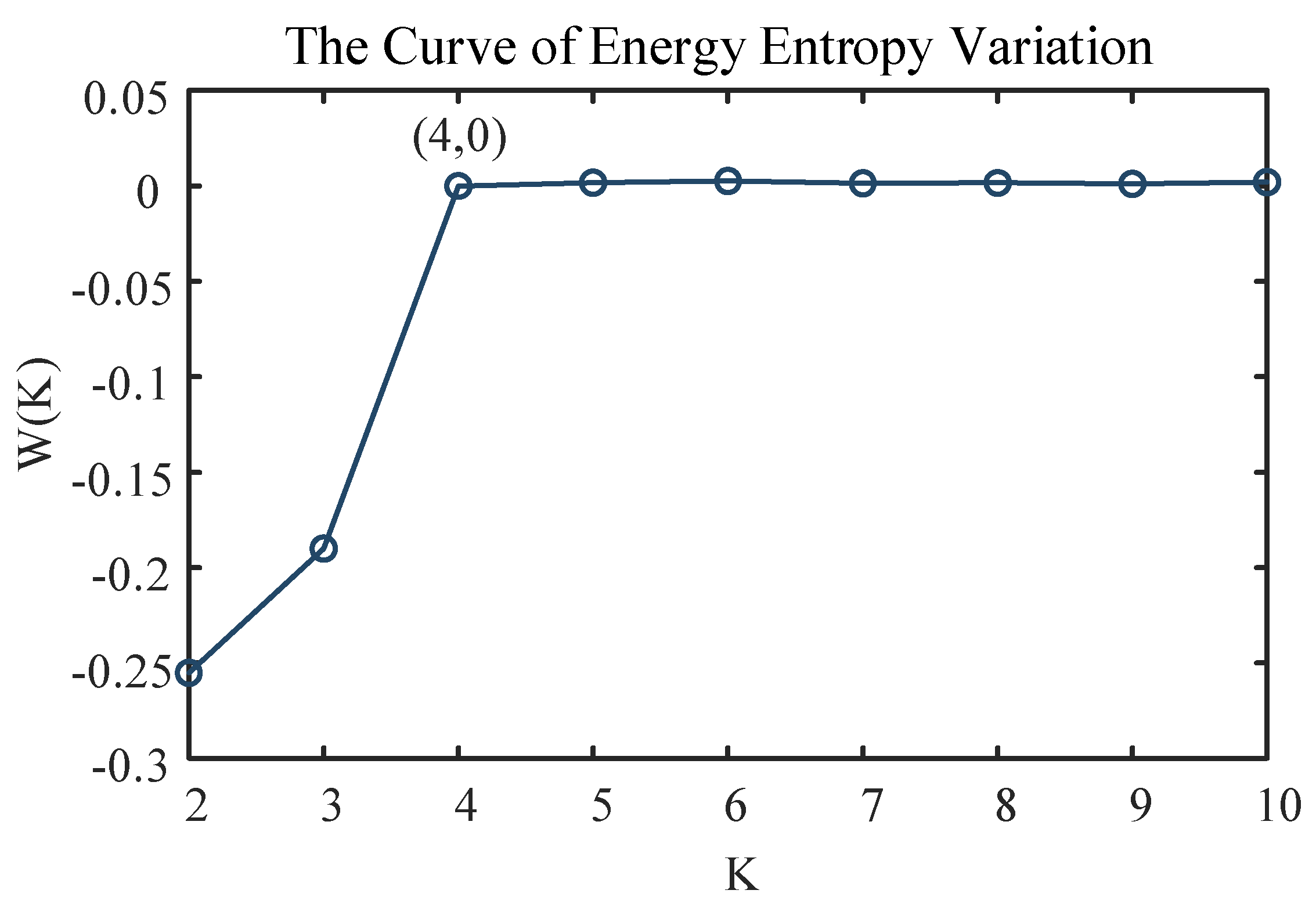
3.1. Variational Mode Decomposition

VMD is a fully non-recursive signal processing method capable of decomposing a multicomponent signal into multiple monocomponent amplitude-frequency modulation (AM-FM) signals in one step. The method effectively extracts key components from signals by adaptively partitioning them in the frequency domain. To achieve efficient decomposition of load equivalent impedance parameters, a constrained variational model of VMD is first constructed. Assume that the original load equivalent impedance parameter sequence can be decomposed into several Intrinsic Mode Functions (IMFs), and its expression is as follows:

$$X_{\mathrm{IMFk}}\left(t\right)=A_{\mathrm{k}}\left(t\right)cos\left({\phi }_{\mathrm{k}}\left(t\right)\right)$$

(8)

where A_k(t) represents the load equivalent impedance parameters R(t) and L(t); $X_{IMFk}\left(t\right)$ is the amplitude of the envelope; and ${\phi }_k\left(t\right)$ is its instantaneous phase.

$$H(t)={‖{\displaystyle \frac{d}{dt}}\left[\left(\mathcal{H}[X_{\mathrm{IMFk}}\left(t\right)]\ast e^{-j{\omega }_{k}t}\right)\right]‖}^2$$

(9)

where ${\omega }_k$ is the central frequency of the k-th mode.

To ensure the effectiveness of Variational Mode Decomposition (VMD), the decomposition process not only minimizes the sum of the estimated bandwidths of each mode (i.e., ensures that each mode is as compact as possible) but also satisfies the constraint that the sum of all modal components equals the original signal to ensure accurate signal reconstruction. These two constraints work together to ensure that the decomposition results are both physically meaningful and maintain signal integrity, and its expression is as follows:

$$\left\{\begin{array}{c}\min {\displaystyle \sum _{k=1}^K\Vert \frac{d}{dt}[(}\mathcal{H}[u_k(t)]\ast e^{-j{\omega }_{k}t})]{\Vert }^2\\ {\displaystyle \sum _{k=1}^K{X}_{\mathrm{IMFk}}\left(t\right)}=A(t)\end{array}\right.$$

(10)

where A(t) is the original load equivalent impedance parameter sequence.

The effect of VMD is mainly influenced by the number of decomposition modes, K. When K is too small, the VMD algorithm cannot fully extract key feature information from the data, thus reducing the accuracy of parameter identification; when K is too large, the central frequencies of adjacent modal components are too close, making the algorithm prone to modal repetition or the introduction of additional noise components. The main difference between different modes is reflected in the central frequencies of their respective Intrinsic Mode Functions (IMFs). Therefore, the optimal K value should be selected as the number of modes at which the central frequency begins to stabilize, ensuring the accuracy and rationality of the decomposition results.

To facilitate the demonstration of central frequency stabilization with the number of decomposition modes, the parameter W(K) is defined by the following equation:

$$W\left(K\right)={\displaystyle \frac{C\_fre\left(K+1\right)-C\_fre\left(K\right)}{C\_fre\left(K\right)}}$$

(11)

where W_fre(K) represents the central frequency corresponding to decomposing the signal into K modes. When the W(K) values of multiple adjacent modes are close to zero, it indicates that the central frequencies of the modes tend to be stable, that is, the mode decomposition results gradually converge. As shown in Figure 2, when plotting the curve of energy entropy variation, it can be observed that the parameter stabilizes and approaches zero after the fourth point. At this stage, the K value for Variational Mode Decomposition (VMD) is selected as 4.

In addition, to more effectively extract the energy characteristics of each modal component, the concept of energy entropy is introduced in this paper. The energy of each modal component and its corresponding energy entropy are expressed as follows:

$$E_i={\displaystyle \int IM{F}_i\left(t\right)dt}$$

(12)

$$H_{EN}=-{\displaystyle \sum }_{i=1}^{K}p{E}_i\lg \left(p{E}_i\right)$$

(13)

where $p{E}_i={\displaystyle \frac{E_i}{{{\displaystyle \sum }}_{i=1}^K{E}_i}}$ is the ratio of the energy of the i-th modal component to the total energy.

3.2. DBSCAN

DBSCAN (Density-Based Spatial Clustering of Applications with Noise) is a clustering algorithm based on the density of sample points [26]. Given the significant differences in the energy and energy entropy of intrinsic modal components of harmonic source loads under different operating states, this algorithm is uniquely suitable for load state identification. The algorithm realizes cluster aggregation by calculating the number of other sample points in the neighborhood of each sample point and introduces two key parameters, Eps and MinPts, to accurately describe the compactness of data samples: Eps defines the maximum distance threshold between two sample points (i.e., the neighborhood radius), and MinPts specifies the minimum number of sample points (including the point itself) that must be contained in the neighborhood of a sample point to determine whether it is a core point. This mechanism can effectively identify clusters of any shape and mark noise points that do not meet the conditions of any cluster, thus significantly improving the accuracy and robustness of load state identification.

The execution process of the DBSCAN algorithm is as follows: First, a sample point that has not been assigned to any cluster is randomly selected from the input dataset. Next, the number of sample points in the Eps neighborhood of this point is calculated: if the number of sample points in the neighborhood reaches or exceeds the MinPts threshold, the point is determined as a core point, and a complete clustering cluster is constructed by iteratively finding all density-reachable sample points; if the number of sample points in the neighborhood is less than MinPts but not zero, the point is defined as a boundary point and can be used as a supplementary member of the cluster formed by adjacent core points; and if there are no other sample points in the neighborhood, the point is determined as a noise point and does not participate in any clustering. The algorithm continues to repeat the above operations until all sample points in the dataset are either clustered or marked as noise. The three data categories of the 2D clustering results based on DBSCAN are shown in Figure 3.

Regarding the selection of the two key parameters, Eps and MinPts, this paper empirically sets MinPts to 10 based on the strong clustering characteristic of modal component energy entropy under the same operating state of the harmonic source load. This setting aims to effectively filter out isolated noise points while preserving true state samples. Referring to [27], Equation (14) is used to estimate the value of Eps. The calculated result indicates that Eps should be set to 0.3754. In this process, the Euclidean distance metric is uniformly adopted to measure the distances between samples.

$$Eps={\left({\displaystyle \frac{{\displaystyle \prod _{i=1}^p}{\left[\max \left(x_i\right)-\min \left(x_i\right)\times MinPts\times \left(0.5\times p+1\right)\right]}^{\frac{1}{p}}}{N\times \sqrt{{\pi }^p}}}\right)}^{{\displaystyle \frac{1}{p}}}$$

(14)

where p denotes the dimensionality of the input feature variables; x_i represents the set of samples for the i-th feature; and n is the total number of clustering samples.

3.3. Operation State Recognition Process

To achieve accurate recognition of the load equipment’s working state, this paper performs Variational Mode Decomposition (VMD) on the load equivalent impedance parameters R(t) and L(t) when the equipment is operating alone. First, the appropriate number of decomposition modes, K, is determined, and then the energy values of each modal component are calculated. Based on the energy values, the energy entropy corresponding to each state is obtained. The acquired modal energy values and energy entropy are integrated to construct a feature matrix, [$E_1,E_2,...,E_k,H_{EN}]$, which serves as the basis for subsequent clustering analysis. Finally, the clustering results are compared and verified with the actual working state of the equipment to evaluate the accuracy and efficiency of the algorithm in load equipment working state recognition. The specific implementation steps are as follows:

• Data Collection and Annotation

Real-time current and voltage data during load operation are collected using measurement equipment, and the current actual working state of the equipment is recorded synchronously to construct an original dataset containing operation parameters and state labels.

2.

Sliding Window Preprocessing

According to the sampling frequency f_m of the measurement equipment and the power frequency f_s of China’s household electricity, the sliding window length is set as w = 10 f_m/f_s to ensure that each window completely covers the data of 10 current cycles, realizing equal-length fragmentation of the original signal.

3.

Variational Mode Decomposition

The VMD algorithm is performed on the data within each sliding window to decompose the complex signal into multiple modal components with different characteristics.

4.

Feature Extraction

Based on Formulas (8)–(13), the energy values and energy entropy of each modal component are calculated, respectively, and a feature vector, T = [$E_1,E_2,...,E_k,H_{EN}]$, is integrated and constructed to achieve the quantitative expression of signal features.

5.

Clustering Analysis

The DBSCAN algorithm is used to cluster the feature vectors, T, of all sliding windows, fusing similar operating states to realize load state recognition.

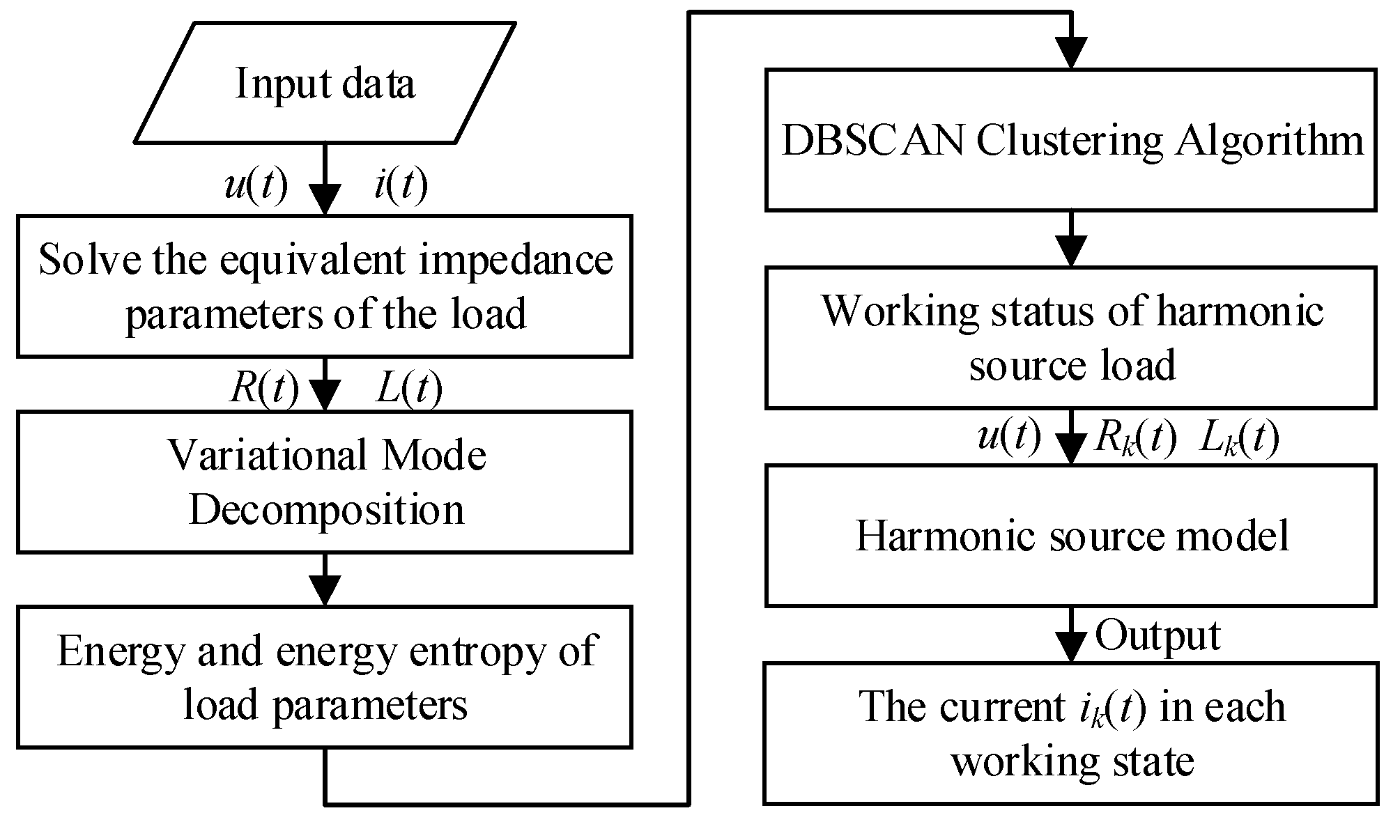
4. The Overall Modeling Process of the Model

This paper proposes a process for constructing a harmonic source load model and identifying its operating state based on load equivalent impedance parameters, as shown in Figure 4. The specific implementation steps are shown below.

Step 1: Data Collection and Sliding Window Preprocessing

High-precision measurement equipment is used to obtain time-domain voltage and current data during load operation. Sliding window technology is adopted to segment and decompose the original data, forming sub-data sequences with time-overlapping characteristics, which provides time-sequentially continuous analysis units for subsequent state identification.

Step 2: State Identification Based on VMD-DBSCAN

The sub-data sequences decomposed by the sliding window are input into the coupled model of Variational Mode Decomposition (VMD) and Density-Based Spatial Clustering of Applications with Noise (DBSCAN). Through VMD’s adaptive frequency-domain decomposition of nonlinear signals combined with DBSCAN’s unsupervised density clustering characteristics, the accurate identification of load working states is realized, and the operating state labels corresponding to each sliding window sub-sequence are determined.

Step 3: Sub-State Equivalent Impedance Modeling

For load data under different working states, an equivalent impedance model is constructed based on circuit theory. The singular value decomposition method is used to solve the equivalent impedance parameters [R, L] corresponding to each state, and a sub-state dynamic model of harmonic source loads is established to achieve the fine-grained characterization of electrical characteristics under different working conditions.

Step 4: State-Matched Current Prediction

For the target load, the measured voltage data are used. Combined with the sub-state equivalent impedance parameters [R, L] established in Step (3), the impedance model of the corresponding working condition is called through the state-matching mechanism, and the model output current is obtained based on Equation (15).

$$\left[\begin{array}{cc}i\left(t_K\right)& {\displaystyle \frac{i\left(t_K\right)}{dt}}\\ i\left(t_{K+1}\right)& {\displaystyle \frac{i\left(t_{K+1}\right)}{dt}}\end{array}\right]=\left[\begin{array}{c}u\left(t_K\right)\\ u\left(t_{K+1}\right)\end{array}\right]{\left[\begin{array}{c}R\left(K\right)\\ L\left(K\right)\end{array}\right]}^{-1}, Kϵ\left[1,2,\cdots N-1\right]$$

(15)

where $u\left(t_K\right)$ and $i\left(t_K\right)$ are the measured voltage data and model output current at time $t_K$, respectively; $R\left(t_K\right)$ and $L\left(t_K\right)$ are the equivalent resistance and reactance parameters at time $t_K$, respectively; the parameters at time $t_{K+1}$ are the same in principle; and n is the window length of the sliding window.

5. Case Studies

5.1. Evaluation Indicators

To comprehensively evaluate the model’s performance, this paper introduces four model evaluation indices, including the state detection accuracy indices, n_wro and n_miss, and the model accuracy indices, namely the Root Mean Square Error (RMSE), Mean Absolute Error (MAE), and Coefficient of Determination (R²). The calculation formulas for the indices are as follows:

$${\mathrm{n}}_{\mathrm{wro}}={\displaystyle \frac{{\mathrm{N}}_{\mathrm{wro}}}{{\mathrm{N}}_{\mathrm{true}}{+\mathrm{N}}_{\mathrm{wro}}}}\times 100\%$$

(16)

$${\mathrm{n}}_{\mathrm{miss}}={\displaystyle \frac{{\mathrm{N}}_{\mathrm{miss}}}{{\mathrm{N}}_{\mathrm{true}}}}\times 100\%$$

(17)

where n_wro represents the false detection rate; n_miss represents the missed detection rate; N_true is the number of actual operating states; N_wro is the number of false detection operating states; and N_miss is the number of missed detection operating states. The closer the calculated values of both the false positive rate and the false negative rate are to zero, the more accurate the state identification results.

$$RMSE=\sqrt{{\displaystyle \frac{1}{n}}{{\displaystyle \sum _{k=1}^n\left(\widehat{i}(k)-i(k)\right)}}^2}$$

(18)

$$MAE={\displaystyle \frac{1}{n}}{\displaystyle \sum _{k=1}^n\left|\widehat{i}(k)-i(k)\right|}$$

(19)

$$R^2=1-{\displaystyle \frac{\sum (\widehat{i}(k)-i(k){)}^2}{\sum (i(k)-\overline{i}{)}^2}}$$

(20)

where $\widehat{i}\left(k\right)$ and i(k) are the k-th actual instantaneous current value and the model output current instantaneous value, respectively; n is the length of the dataset. Among them, the smaller the values of the MAE and RMSE, and the closer R² is to 1, the more accurate the parameter solution result.

5.2. Validation with Simulation Data

To verify the effectiveness of the load identification and modeling method, this section presents a single-phase load simulation model built for asymmetric loads in the Matlab/Simulink environment. The power supply voltage is set according to the national standard for commercial power, with an effective value of 220 V, a frequency of 50 Hz, and a sampling frequency of 10 kHz. Sampling points are arranged at the load input terminal to collect single-phase voltage and current data, which are processed and analyzed using Matlab R2024a.

To simulate actual operating scenarios, this paper sets up different scenarios of load equivalent impedance parameters to verify the method, with specific scenario configurations listed in

Table 1. Load equivalent impedance parameters in each state.

State	Title 2	Title 3
1	R	15 Ω
	L	0.01 H
2	R	200 Hz 10 to 20 Ω sine waves
	L	50 Hz 0.01 to 0.02 H square wave
3	R	50 Hz 10 to 20 Ω square waves
	L	200 Hz 0.01 to 0.02 H sine waves
4	R	200 Hz 10 to 20 Ω sine waves
	L	200 Hz 0.01 to 0.02 H sine waves

. Among them, State 1 simulates equivalent impedance parameters under steady-state conditions to analyze the identification effect of the proposed method when load impedance equivalent parameters remain constant. States 2 and 3 leverage the characteristic that square wave signals contain only high/low discrete values to construct simulation conditions for single-parameter gradual change and abrupt change, respectively. The former is used to verify the dynamic response of the method to slowly varying parameters, while the latter tests the recognition sensitivity to discontinuous parameter mutations. State 4 further establishes a composite condition with synchronous changes in multiple parameters, evaluating the method’s identification performance under continuously time-varying parameters. These four scenarios comprehensively verify the method’s capability to identify different load operating states, ensuring its adaptability to diverse operational scenarios in practical applications.

In the experiment, 300 sets of load voltage and current sampling data were selected for modeling, with 150 data points used as the validation set. First, the load equivalent impedance parameters under different states were calculated using singular value decomposition (SVD), and the Z-score criterion was applied to identify and replace parameter outliers. To demonstrate the applicability of the Z-score criterion, both the Z-score (with a threshold of ±3.5) and IQR (interquartile range, with a multiplier of 1.5) were applied to process the simulated data of State 3 in the table, and their impacts on the modeling results were compared and analyzed. In this scenario, the resistance, R, was set to switch between 10 Ω and 20 Ω as a 50 Hz square wave, while the inductance, L, varied between 0.01 H and 0.02 H as a 200 Hz sine wave. Additionally, Gaussian-distributed noise was introduced to simulate real-world operating conditions. The results are shown in

Table 2. Comparison of RMSE under State 3 scenario using different outlier handling methods.

Method	RMSE	Error Increase Compared to Z-Score
Z-score	3.3601	-
IQR	3.8927	013.7%

. The RMSE of the model after Z-score processing was 3.3601, which is 13.7% lower than that obtained using the IQR (3.8927). This improvement was achieved because the Z-score method characterizes data distribution through its central tendency and dispersion, enabling more accurate capture of feature variations in non-normally distributed data. In contrast, the IQR method relies on fixed multiples of the interquartile range, which may lead to missed detection of outliers when dealing with asymmetric distributions containing high-frequency abrupt changes due to an overly broad coverage of the quantile interval. Therefore, the Z-score criterion demonstrates superior performance in dynamic load parameter identification scenarios.

Table 3. Evaluation of State Recognition Accuracy with Simulated Data.

Working State	State 1	State 2	State 3	State 4
nwro	0	0.2	0.15	0.04
nmiss	0	0	0.17	0.2

shows the evaluation of state recognition accuracy with simulated data. The results indicate that for Simulink simulation data, the method demonstrates excellent performance in operating state determination. Especially in Scenario 1 (linear load), the method exhibits superior identification stability, with both the n_wro and n_miss values being 0, indicating completely accurate state determination for loads with constant parameters. When load parameters undergo gradual (State 2) or abrupt (State 3) changes, the n_wro and n_miss values increase slightly but remain below 0.17, verifying the method’s high identification accuracy under dynamic conditions. Additionally, in State 4 with synchronous continuous changes in multiple parameters, the method maintains n_wro and n_miss values below 0.2, demonstrating strong adaptability to complex operating conditions.

Through simulation verification of four typical scenarios, the proposed method shows high identification accuracy and stability in steady-state identification, dynamic response, and composite change scenarios of load equivalent impedance parameters. It achieves zero false detection and zero missed detection in linear load states and controls the false detection and missed detection probabilities within 2.4% in parameter change scenarios, fully proving its effectiveness.

To verify the modeling accuracy, this section introduces harmonic source modeling methods of HCAM [28] and LS-SVM [29] for comparative experiments. The modeling results of each working state are shown in Figure 5, and the model accuracy indices are detailed in

Table 4. Verification of Model Accuracy with Simulated Data.

State	Indicator	Proposed Method	HCAM	LS-SVM
1	MAE	0.7366	2.3041	4.8973
	RMSE	0.8226	2.5591	5.4191
	R2	0.9977	0.9775	0.8991
2	MAE	2.6163	2.8782	5.2376
	RMSE	3.2128	3.7058	6.1614
	R2	0.9666	0.9557	0.8774
3	MAE	2.8253	3.2998	5.86
	RMSE	3.3601	3.778	7.0667
	R2	0.9686	0.9603	0.8611
4	MAE	2.9031	2.6387	5.5608
	RMSE	3.795	3.387	6.3409
	R2	0.9554	0.9645	0.8756

. The results indicate that the proposed method demonstrates significant advantages under all operating conditions. Compared with the HCAM method, the modeling error (MAE) of the proposed method is reduced by 9.10–68.03% under operating states 1–3, while the coefficient of determination, R², increases by 0.0083–0.0202. This improvement mainly stems from the fact that the HCAM method relies on parameter assumptions based on mechanistic modeling, making it difficult to accurately characterize complex nonlinear loads with unknown structures. In comparison with the LS-SVM method, the proposed method reduces the modeling error (MAE) by 47.79–84.96% (with reductions exceeding 30% in all cases) and improves the R² metric by 0.0798–0.1075 across all operating conditions. The limitations of LS-SVM lie in its tendency to overfit and thus exhibit poor generalization performance in small-sample scenarios, along with a lack of physical interpretability of its model parameters. In contrast, the proposed method retains more complete characteristic information of the harmonic source load and directly describes the load’s current response in the time domain without requiring time-frequency transformation. This avoids potential information loss inherent in models like HCAM and effectively prevents overfitting. Moreover, the model parameters offer clearer physical meaning. In summary, the harmonic source model proposed in this paper demonstrates strong versatility and high modeling accuracy, making it suitable for various types of harmonic source loads and offering notable advantages over existing modeling approaches.

5.3. Verification with Measured Data

To verify the practicality of the load identification and modeling method, this paper addresses challenges such as deviations between Simulink simulation data and actual operating conditions, annotation gaps in public datasets (PLAID/AMPds/BLUED), and insufficient independent device data by constructing a standardized test platform. The DEWETRON DEWE-5000 data acquisition system was employed, with a stabilized supply voltage of 220 ± 2.2 V and 50 ± 0.05 Hz, to capture voltage and current data from harmonic source loads at a 10 kHz sampling rate across full operational conditions.

5.3.1. Effectiveness Verification of Operating State Identification

To verify the effectiveness of the load identification method, this paper selects typical household appliances, such as a hairdryer (Hai), fan, microwave (Mic), and laptop (Lap), and conducts an analysis combined with laboratory measured data. As shown in Figure 6, for finite-state devices with clear discrete working states (such as hairdryers), the proposed method can accurately identify four operating modes: low cool, low hot, and high hot. From the perspective of the recognition accuracy evaluation indicators in

Table 5. Identification results of measured data.

Working State	Hai	Fan	Mic	Lap
nwro	0	0	1.9	3.1
nmiss	0	0	2.4	2.3

, the method performs excellently in state identification, especially in the operational state monitoring of low-power harmonic source loads, with the highest relevant indicator being only 3.1%. This fully verifies the method’s effective identification capability for the characteristic current modes of various load devices, providing important practical value and reference significance for the state-separated modeling of harmonic source loads. Additionally, for continuously variable state loads (such as electric fans and microwave ovens), the VMD-DBSCAN algorithm is adopted to effectively classify similar operating states. The experimental results show that the method can not only accurately identify the discrete working conditions of finite-state devices (such as the four operating modes of hairdryers) but also properly handle the fuzzy characteristics of continuously variable state loads through clustering analysis, demonstrating good adaptability and robustness to diversified load scenarios.

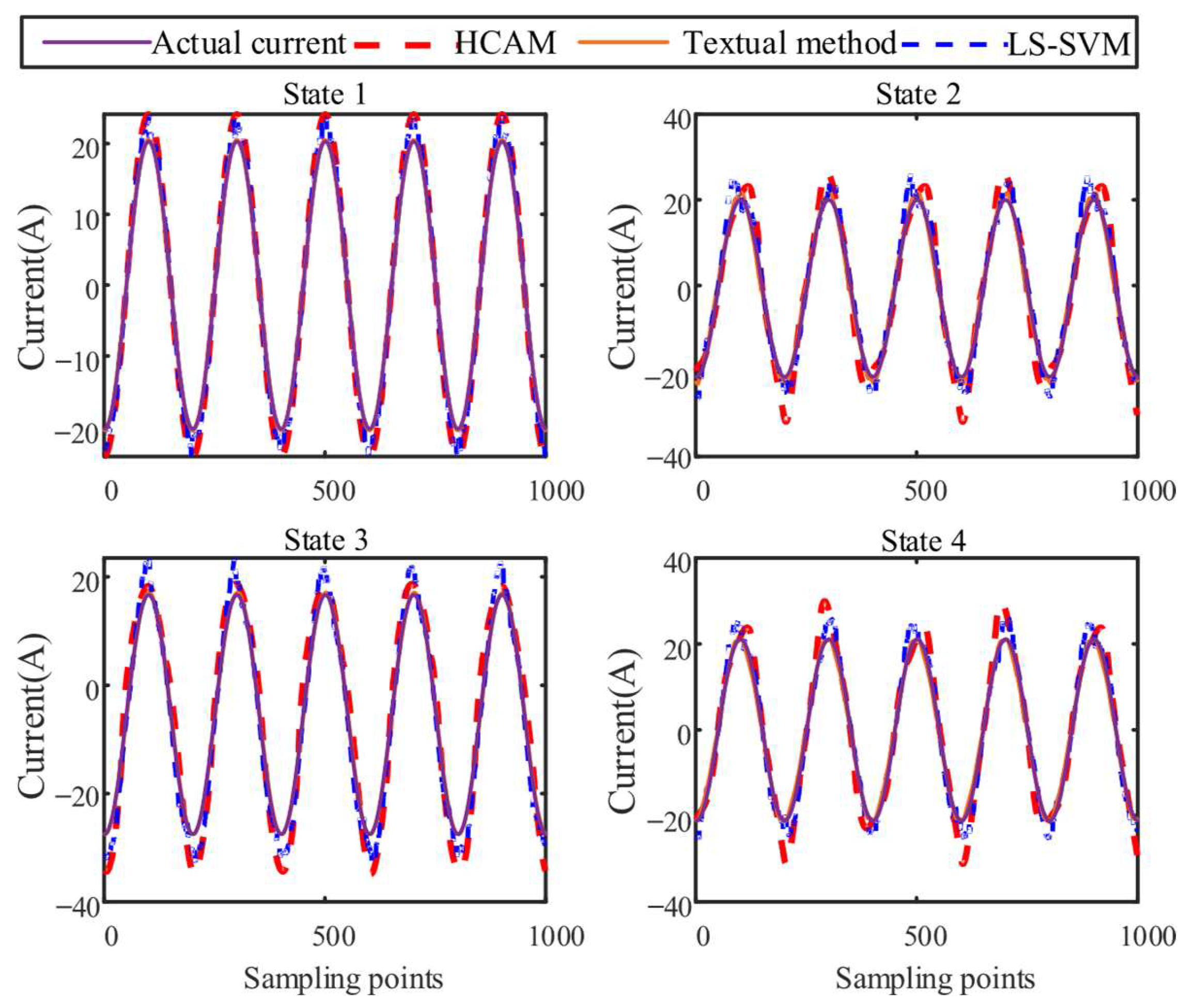
5.3.2. Model Validity Verification

Based on the classification results, a state-separated harmonic source load model based on load equivalent impedance parameters is established. Figure 7 shows the output current waveforms of the proposed model and comparative models versus the actual current, with relevant evaluation indices listed in

Table 6. Accuracy index of measured data.

Working State	Textual Method		HCAM		LS-SVM
	MAE	RMSE	MAE	RMSE	MAE	RMSE
Fan a	0.1725	0.2006	0.2221	0.2446	0.2187	0.2630
Fan b	0.7786	0.9597	0.9881	1.1127	0.9436	1.0974
Fan c	1.3676	1.6761	1.7281	1.9522	1.6567	1.9258
Fan d	0.9248	1.1199	0.7836	0.9001	0.9114	1.1799
Hai a	0.0135	0.0162	0.0263	0.0297	0.0139	0.0163
Hai b	0.0258	0.0285	0.0258	0.0289	0.0174	0.0195

. It can be seen that among the 12 groups of comparative data, the proposed model outperforms both HCAM and LS-SVM in terms of the MAE and RMSE in 10 groups. Although the MAE of the proposed model in Lap d state is slightly higher than that of HCAM, its RMSE (1.1199) is still lower than HCAM’s 0.9001, indicating that the model prioritizes overall error control when handling non-steady-state data. Additionally, the R² index of the proposed model is generally higher than that of comparative models, further verifying its stronger interpretability of load characteristics.

In summary, the harmonic source model proposed in this paper demonstrates strong generality, is suitable for various harmonic source loads, and exhibits higher accuracy compared with other comparative models.

6. Conclusions

This paper proposes a harmonic source load model and operating state determination method based on load equivalent impedance parameters. The method is verified through simulation and measured data, leading to the following conclusions: (1) A dynamic load modeling method based on an RL-series equivalent impedance model is proposed. This approach accurately characterizes the dynamic behavior of loads in the time domain through time-varying impedance parameters, R(t) and L(t), providing a theoretical foundation and technical support for key steps such as load operating state identification and state-based modeling. The method effectively overcomes the limitations of traditional mechanistic models in terms of applicability, as well as the lack of physical interpretability in purely data-driven models. It establishes a modeling framework for harmonic source loads that combines clear physical principles with engineering practicality. (2) The proposed operating state determination method integrates Variational Mode Decomposition (VMD) and Density-Based Spatial Clustering of Applications with Noise (DBSCAN) algorithms to achieve high-precision identification and feature extraction of asymmetric load operating states. By dividing historical sample sets under different working conditions into multiple sub-sample sets, the adaptability and generalization ability of the harmonic source model to global samples are significantly enhanced. (3) The proposed model is applicable to a wide variety of harmonic source loads, offering high accuracy and strong generalization capability. It serves as a fundamental tool for power system harmonic power flow analysis, harmonic responsibility allocation, and power quality assessment. This model provides more reliable data support for grid planning, operation, and regulation, facilitating the development of targeted harmonic management strategies and enabling the optimization of power quality at its source.

References

1. Wang, Y.; Yong, J.; Sun, Y.; Xu, W.; Wong, D. Characteristics of harmonic distortions in residential distribution systems. IEEE Trans. Power Deliv. 2017, 32, 1495–1504. [Google Scholar] [CrossRef]
2. Xu, D.; Wang, F.; Mao, H.; Ruan, Y.; Zhang, W. Modeling and analysis of harmonic interaction between multiple grid-connected inverters and power grid. Proc. CSEE 2013, 33, 64–71. [Google Scholar]
3. Li, Y.; Sun, Y.; Wang, Q.; Sun, K.; Li, K.-J.; Zhang, Y. Probabilistic harmonic forecasting of the distribution system considering time-varying uncertainties of the distributed energy resources and electrical loads. Appl. Energy 2023, 329, 120298. [Google Scholar] [CrossRef]
4. Wang, Y.; Yang, Y.; Ma, X.; Yao, W.; Wang, H.; Tang, Z. Unbalanced responsibility division considering renewable energy integration. IET Gener. Transm. Distrib. 2020, 14, 6000–6008. [Google Scholar] [CrossRef]
5. Liao, Y.; Hu, J.; Zhang, H.; Wang, E. Time-varying parameter model of AC arc furnace for power quality prediction and analysis. Electr. Technol. 2016, 17, 41–46. [Google Scholar]
6. Wang, Y.; Jiang, J. A new chaotic model of AC arc furnace for power quality research. Proc. CSEE 2008, 28, 106–110. [Google Scholar]
7. Li, Q.; Cheng, P.; Wang, W. Modeling and analysis of harmonic current in middle-frequency band in DFIG based wind turbines. Autom. Electr. Power Syst. 2018, 42, 41–47. [Google Scholar]
8. Moreno, M.A.; Usaola, J. A new balanced harmonic load flow including nonlinear loads modeled with RBF networks. IEEE Trans. Power Deliv. 2004, 19, 686–693. [Google Scholar] [CrossRef]
9. Zhao, Y.; Milanović, J.V. Equivalent modelling of wind farms for probabilistic harmonic propagation studies. IEEE Trans. Power Deliv. 2022, 37, 603–611. [Google Scholar] [CrossRef]
10. Marulanda-Durango, J.; Escobar-Mejía, A.; Alzate-Gómez, A.; Álvarez-López, M. A support vector ma-chine-based method for parameter estimation of an electric arc furnace model. Electr. Power Syst. Res. 2021, 196, 107228. [Google Scholar] [CrossRef]
11. Luo, X.; Zhang, D.; Zhu, X. Combining transfer learning and constrained long short-term memory for power generation fore casting of newly-constructed photovoltaic plants. Renew. Energy 2022, 185, 1062–1077. [Google Scholar] [CrossRef]
12. Zhan, Y.; Cheng, H.; Ge, N.; Huang, G. Generalized growing and pruning rbf neural network based harmonic source modeling. Proc. CSEE 2005, 25, 42–46. [Google Scholar]
13. Xie, K.; Yang, H.; Zhang, Y.; Huang, J. Harmonic source modeling based on generalized regression neural network. Adv. Technol. Electr. Eng. Energy 2012, 31, 64–67. [Google Scholar]
14. Zheng, L.; Wu, P.; Liu, X. Application of least squares support vector machine to harmonic sources modeling based on genetic algorithm. Power Syst. Prot. Control. 2011, 39, 52–56. [Google Scholar]
15. Zhang, Y.; Liu, B.; Shao, Z.; Lin, F.; Lin, C. General and uncertain harmonic source model based on Gaussian process regression. Proc. CSEE 2021, 42, 992–1001. [Google Scholar]
16. Shao, Z.; Lin, K.; Chen, J.; Pan, X. Typical modes analysis of harmonic customers based on the interval arithmetic. J. Electr. Power Sci. Technol. 2018, 33, 153–160. [Google Scholar]
17. Liu, Q.; Yin, W.; Hu, W.; Tao, S. Prediction of power harmonic monitoring data based on LSTM algorithm. Power Capacit. React. Power Compens. 2019, 40, 139–145. [Google Scholar]
18. Gao, P.; Fang, J.; Han, Y.; Wang, J. Analysis and prediction of power quality trend of electrified railway. Comput. Digit. Eng. 2019, 47, 1521–1527. [Google Scholar]
19. Sun, M.; Zhang, T.; Wang, Y.; Strbac, G.; Kang, C. Using Bayesian deep learning to capture uncertainty for residential net load forecasting. IEEE Trans. Power Syst. 2020, 35, 188–201. [Google Scholar] [CrossRef]
20. Wang, Y.; Zang, T.; Fu, L.; Zheng, Z. Adaptive method for dynamic harmonic state estimation in power system based on feature extraction of harmonic source. Power Syst. Technol. 2018, 42, 2612–2619. [Google Scholar]
21. Fauri, M. Harmonic modelling of non-linear load by means of crossed frequency admittance matrix. IEEE Trans. Power Syst. 1997, 12, 1632–1638. [Google Scholar] [CrossRef]
22. Zhang, Y.; Chen, S.; Liu, B.; Lin, C. Industrial Harmonic Source Load Classification Recognition Method Based on Blind Source Separation. Proc. CSEE 2024, 44, 3850–3862. [Google Scholar]
23. Tang, K.; Cai, M.; Luo, J.; Zhu, B.; Tan, T. Harmonic Source Localization Method for Nonlinear Loads Based on Singular Value Decomposition. Autom. Electr. Power Syst. 2012, 36, 96–100. [Google Scholar]
24. Tang, K.; Shen, C.; Liang, S.; Huang, X. Outlier issues in harmonic source location based on parameter identification method. In Proceedings of the 2016 IEEE Power and Energy Society General Meeting (PESGM), Boston, MA, USA, 17–21 July 2016; IEEE: Piscataway, NJ, USA, 2016. [Google Scholar] [CrossRef]
25. Hosking, J.R. L-moments: Analysis and Estimation of Distributions using Linear Combinations of Order Statistics. J. R. Stat. Society. Ser. B (Methodol.) 1990, 52, 105–124. [Google Scholar] [CrossRef]
26. Zhang, D.Z.; Li, K.Q.; Wang, J.Q. A curving ACC system with coordination control of longitudinal car-following and lateral stability. Veh. Syst. Dyn. 2012, 50, 1085–1102. [Google Scholar] [CrossRef]
27. Chu, Y.; Chen, H.; Wang, J.; Wu, Y.; Lei, A. Complex Signal Harmonic Source Modeling Method Based on Multivariate Gaussian Process Regression and DBSCAN Algorithm. Trans. China Electrotech. Soc. 2025, 1–15. [Google Scholar] [CrossRef]
28. Nassif, A.B.; Yong, J.; Xu, W. Measurement-based approach for constructing harmonic models of electronic home appliances. IET Gener. Transm. Distrib. 2010, 4, 363–375. [Google Scholar] [CrossRef]
29. Li, B.; Wu, P.; Liu, X.; Zheng, L. Harmonic source modeling based on least squares support vector machine. Electr. Energy Manag. Technol. 2010, 4, 58–62. [Google Scholar]
Figure 1. Schematic diagram of time-domain load equivalent impedance parameters.
Symmetry 17 01123 g001
Figure 2. The curve of energy entropy variation.
Symmetry 17 01123 g002
Figure 3. Three types of data points in DBSCAN algorithm.
Symmetry 17 01123 g003
Figure 4. Overall modeling flowchart.
Symmetry 17 01123 g004
Figure 5. Prediction results of load model.
Symmetry 17 01123 g005
Figure 6. Multi-state current waveform of harmonic source loads.
Symmetry 17 01123 g006
Figure 7. Prediction results of fan.
Symmetry 17 01123 g007