Article

Geometric Accumulation Operators of Dombi Weighted Trapezoidal-Valued Fermatean Fuzzy Numbers with Multi-Attribute Group Decision Making

1
Department of Mathematics, Vel Tech Rangarajan Dr. Sagunthala R&D Institute of Science and Technology Avadi, Chennai 600062, Tamil Nadu, India
2
Department of Basic Sciences, College of Science and Theoretical Studies, Saudi Electronic University, P.O. Box 93499, Riyadh 11673, Saudi Arabia
*
Authors to whom correspondence should be addressed.
Symmetry 2025, 17(7), 1114; https://doi.org/10.3390/sym17071114
Submission received: 10 June 2025 / Revised: 4 July 2025 / Accepted: 6 July 2025 / Published: 10 July 2025
(This article belongs to the Topic Fuzzy Sets Theory and Its Applications)

Abstract

Trapezoidal-valued fermatean fuzzy numbers (TpVFFNs) are essential for handling daily decision-making issues in the engineering and management fields. Accumulation processes on the set of TpVFFN are used to address decision-making problems described in this environment as necessary. The primary goal of this paper is to provide the concept of Dombi t-norm ( D t n ) - and Dombi t-conorm ( D t c n ) -based accumulation operators on the class of TpVFFN, emphasizing how they behave symmetrically in aggregation processes to maintain consistency and fairness. To use s to illustrate mathematical circumstances, we first create a trapezoidal-valued fermatean fuzzy Dombi’s weighted geometric operator, hexagonal hybird geometric operator, fermatean fuzzy order weighted geometric operator. Second, we use a multi-attribute group decision-making (MAGDM) approach to compute the recommended accumulation operators. Finally, we demonstrate the potential practical application of the proposed decision-making problem related to the pink cab.

1. Introduction

The fuzzy set theory, which maintains that the sum of the degrees of membership and non-membership equals 1, was initially put forth by Zadeh [1]. The concept of an intuitionistic fuzzy set (IFS), in which the sum of the degrees of membership or non-membership of each element is equal to one, was developed by Atanassov [2]. Smarandache [3] elaborates on neutrosophic sets and various functions. Ye [4] introduces single-valued neutrosophic linguistic numbers (SVNLNs) and sets (SVNLSs) as extensions of linguistic and intuitionistic linguistic concepts. To handle disputed, unclear, and partial data in MADM, Chi and Liu [5] extend the TOPSIS technique to interval neutrosophic sets (INSs). We offer an enhanced approach that considers INS-valued qualities with uncertain weights, as traditional TOPSIS relies on exact quantities. We outline INS processes, introduce a distance measure, and compute attribute weights using the maximizing deviation methodology. A created model that was used for additional levels later demonstrated the effectiveness of these extended TOPSIS phases. For neutrosophic fuzzy sets, Bui et al. [6] offer entropy-based measures and an updated decision-making process. It outperforms previous methods when used to select courses for high school examinations in Vietnam; the code is available on GitHub (4.4 Open source codes) and the outcomes are carefully reviewed. Innovative Hausdorff distance measures for single-valued neutrosophic sets are proposed by Ali et al. [7] and used for multi-criteria decision making (MCDM).

1.1. Review of the Literature

The D t n and D t c n operations were introduced by Dombi [8], who also discussed certain properties of operators. Liu et al. [9] develop the use of Dombi operations on IFSs to address real-world problems. Seikh and Mandal explain and use IF Dombi accumulation methods for judgments involving several characteristics in [10]. In addition to proposing a neutrosophic cubic Dombi weighted arithmetic average operator and geometric average operator, this study extends the Dombi operations to neutrosophic cubic sets. In [11], Shi and Ye spoke about how to address decision-making issues in neutrosophic cubic contexts with adjustable operating parameters. The EDAS approach was extended to fuzzy sets with a q-rung orthopair by Shao & Zhuo [12], who also investigated its suitability for evaluating the disposal of biological waste. Deveci et al. [13] assessed the integration of many fluidity measurement approaches using the fuzzy Dombi evaluation based on the distance from the average solution (EDAS) model. The D t n and D t c n methods of the image fuzzy set environment were introduced by Jana et al. [14]. Furthermore, geometric/arithmetic accumulation approaches for image Dombi were established. A comprehensive and well-structured analysis of MADM techniques for decision-making difficulties covering the years 2004–2024 was presented by Kumar and Pamucar [15]. A few well-known publications in the literature tackle MCDM issues using classes of fuzzy accumulation operators. Ali et al. [16] also examined a method that uses intuitionistic fuzzy soft information and Aczel–Alsina operational laws to solve multi-attribute problems in MCDM, while Asif et al. [17] employed Hamacher accumulation procedures to solve multi-attribute problems in the Pythagorean fuzzy set. A research study conducted for MCDM applications to handle energy management issues between 2010 and 2025 is examined by Sahoo et al. [18], which is one of the primary categories encompassing today’s global problems. Naeem and Ali have discussed the Aczel–Alsina spherical fuzzy accumulation operator-based multi-criteria group decision making (MCGDM) and its application in evaluating solar energy cells [19]. Using the interval-valued intuitionistic fuzzy number, interval-valued trapezoidal neutrosophic set, score, and accuracy functions utilized in the proposed study, Khatter [20] explored several operational principles based on this combination. Drawing from the ideas of a modified uncertainty index and an enhanced value index, Nayagam, Jeevaraj, and Dhanasekaran [21] introduced a unique method for taking into account trapezoidal-valued intuitionistic numbers. An enhanced algorithm for addressing MADM issues is created. Application of Dombi weighted geometric aggregation operators in MAGDM for the class of trapezoidal-valued intuitionistic fuzzy numbers was introduced by Meher et al. in [22]. To address the drawbacks of some of the current ranking techniques, Bihari et al. in [23] provide a unique ranking concept based on the diagonal distance and mean score function. They also show how effective the proposed model is as a tool for choosing MCDM providers in an uncertain setting.
Senapati and Yager [24] proposed fermetean fuzzy sets (FFSs), a novel kind of FSs. FFSs are composed of both membership and non-membership degrees, which meet this 0 ( Φ A ( x ) ) 3 + ( Ψ A ( x ) ) 3 1 condition; therefore, it precisely manages the aforementioned situations. Mishra and Rani [25] proposed the weighted aggregated sum product assessment (WASPAS) method in the context of FFSs. While Garg et al. [26] demonstrated how to use FFs in a COVID-19 testing facility, Yang et al. [27] investigated the continuities and derivatives of FF functions. Sergi and Sari proposed a few FF capital budgeting strategies [28]. Sahoo [29] suggested a few FFS scoring functions and their applications to transportation-related issues and decision making.
To better manage uncertainty and attribute interrelationships in MCDM, Wu et al. [30] developed innovative interval-valued intuitionistic fuzzy (IVIF) Dombi–Hamy mean operators. They used these operators to assess the quality of services provided by senior tourism, showing enhanced accuracy and flexibility in fuzzy aggregation. Pure and non-pure rational decision-making techniques were presented by Lu and Cheng [31] in interval-valued fuzzy soft β -covering approximation spaces. By incorporating logic into the decision-making process, their method improves uncertainty handling in fuzzy soft set situations. A sophisticated framework for multi-attribute decision making in intricate fuzzy situations is presented in this paper.
In order to improve the representation of uncertainty, Torra [32] originally proposed the use of hesitant fuzzy sets (HFSs) to depict scenarios in which decision-makers waver between several membership values. Lu, Xu et al. [33] expanded on this by creating hesitant fuzzy information systems (HFISs) and basic theories, which they then used to intelligent classifiers. Their research greatly broadens the use of HFSs in AI and multi-attribute decision-making scenarios. Senapati et al. [34,35] improved the modeling of uncertainty in complicated decision making by creating IVIF aggregation operators based on Aczel–Alsina operations. For situations involving the decision making of several attributes, their work offers strong tools and also examines Aczel–Alsina geometric aggregation operators in a related work, demonstrating the usefulness and efficiency of these techniques in unpredictable situations.
HFSs capture expert judgment hesitancy and improve qualitative decision-making flexibility by allowing the membership degree of an element to be represented by a collection of potential values. On the other hand, trapezoidal-valued fuzzy numbers (TpVFNs) offer a precise method of modeling uncertainty in numerical or interval-based data by defining a trapezoidal membership function using four parameters. TpVFNs are more appropriate for tasks needing organized numerical fuzziness, whereas HFSs are best suited for subjective or linguistic judgments containing ambiguity.

1.2. Research Gap

The generality and usefulness of fermatean fuzzy numbers (FFNs), despite progress in fuzzy set theory and its applications to MADM. Triangular FFNs (TFFNs) and interval-valued FFNs (IVFFNs) are not adequately captured or extended by the current paradigm of conventional trapezoidal fermatean fuzzy numbers (CTpFFNs). The structural definitions of CTpFFNs violate the fundamental requirements for fuzzy set generalization as they are not mathematically consistent when simplified. Furthermore, no previous study has integrated D t n and D t c n operations into the framework of TpVFFNs, despite the fact that these procedures have demonstrated promise in a variety of fuzzy settings, including intuitionistic and neutrosophic sets. Moreover, current methods often fail to ensure algebraic or structural symmetry in operator behavior, which might result in bias or inconsistent multi-attribute assessments. A methodological gap in creating adaptable, precise, and adjustable aggregation operators appropriate for the TpVFFN structure has resulted from this drawback. Furthermore, there are currently few tools that can fully utilize the expressive potential of TpVFFNs in complicated decision-making scenarios, as most MADM models under fuzzy logic settings are designed to fit more traditional or constrained fuzzy set forms.

1.3. Motivation and Contribution of the Study

The TpVFFNs offer a valid and mathematically coherent generalization of several fuzzy number types, such as real-valued FFNs, TFFNs, and IVFFNs, which is what inspired this work. More accurate depictions of ambiguity and uncertainty are made possible by this framework. In this context, Dombi aggregation operators are especially appealing because of their configurable parameters, which allow for more flexibility and adaptability than conventional set t-norms. The suggested operators improve the model’s interpretability and mathematical consistency by maintaining algebraic symmetry through commutative features. Furthermore, the study improves the accuracy and dependability of decision results by placing these operators into a MADM framework and using a comprehensive ordering principle in the TpVFFN environment. The practical case study—choosing the best pink taxi services—showcases the usefulness and practicality of the suggested techniques, highlighting their potential for greater usage in the domains of operation research, management, and engineering.

1.4. Significance of the Research

  • On the basis of D t n and D t c n , we contribute specific TpVFFN procedures.
  • For the TpVFFN class, we propose three accumulation procedures: TpVFFDWG, TpVFFDOWG, and TpVFFDHG.
  • We create a trapezoidal-valued fermetean fuzzy MAGDM (TpVFFMAGDM) algorithm using the recommended operators.

1.5. Organization of This Paper

This paper’s remaining sections are arranged as follows. A few fundamental introductions and definitions are given in Section 2. Section 3 proposes a few operating rules for TpVFFNs based on D t n and D t c n . TpVFFDWG, TpVFFDOWG, and TpVFFDHG are the three geometric mean-based Dombi accumulation operators that are introduced in Section 4. Section 5 outlines the TpVFFMAGDM method, based on accumulation operators and an application of MAGDM to solve the decision-making issues related to pink cabs. Lastly, Section 6 provides the conclusions.

2. Preliminaries

Definition 1 
([8]). Let a t p and b t p be a real number; then, D t n and D t c n of the TpVFFNs are characterized by
D t n ( x t p , y t p ) = 1 1 + { ( 1 a t p 3 a t p 3 ) γ T p V + ( 1 b t p 3 b t p 3 ) γ T p V } 1 γ T p V 3
and
D t c n ( x t p , y t p ) = 1 1 1 + { ( a t p 3 1 a t p 3 ) γ T p V + ( b t p 3 1 b t p 3 ) γ T p V } 1 γ T p V 3
, where γ T p V > o and a t p , b t p [ 0 , 1 ] × [ 0 , 1 ] . The Dombi operating parameter is γ T p V .
Definition 2 
([2]). Let A T p V be a nonvoid set. An IFS X T p V in A T p V is characterized by X T p V = { x t p , β X T p V ( x t p ) , υ X T p V ( x t p ) | x t p A T p V } , where β X T p V : A T p V [ 0 , 1 ] and υ X T p V : A T p V [ 0 , 1 ] , x t p A T p V with the conditions 0 β X T p V ( x t p ) + υ X T p V ( x t p ) 1 . The numbers β X T p V ( x t p ) , υ X T p V ( x t p ) [ 0 , 1 ] .
Definition 3 
([24]). Let S t p ( 0 , 1 ) be the set of all trapezoidal fuzzy numbers in [0,1]. A trapezoidal-valued intuitionistic fuzzy set on a set A T p V is given by the expression X T p V = { x t p , β X T p V ( x t p ) , υ X T p V ( x t p ) | x t p A T p V } , where β X T p V : A T p V S t p ( 0 , 1 ) , υ X T p V : A T p V S t p ( 0 , 1 ) with the condition 0 < s u p x t p β X T p V ( x t p ) + s u p x t p υ X T p V ( x t p ) < 1 . The T p V F F N s β X T p V ( x t p ) and υ X T p V ( x t p ) denote the element x t p to be included in the collection X T p V , both its membership degree and non-membership degrees. Therefore, for each x t p A T p V , β X T p V ( x t p ) and υ X T p V ( x t p ) are trapezoidal-valued intuitionistic fuzzy numbers represented by β X T p V L ( x t p ) , β X T p V m 1 ( x t p ) , β X T p V m 2 ( x t p ) , β X T p V U ( x t p ) and υ X T p V L ( x t p ) , υ X T p V m 1 ( x t p ) , υ X T p V m 2 ( x t p ) , υ X T p V U ( x t p ) . Thus, we have
X T p V = { x t p , ( β X T p V L ( x t p ) , β X T p V m 1 ( x t p ) , β X T p V m 2 ( x t p ) , β X T p V U ( x t p ) ) , ( υ X T p V L ( x t p ) , υ X T p V m 1 ( x t p ) , υ X T p V m 2 ( x t p ) , υ X T p V U ( x t p ) ) : x t p A T p V }
where 0 β X T p V ( x t p ) + υ X T p V ( x t p ) 1 . The set of T p V F F S in A T p V is denoted by T p V F F S ( A T p V ) . In general, any T p V F N is denoted by A ^ t p = ( a ^ t p , b ^ t p , c ^ t p , d ^ t p ) , ( e ^ t p , f ^ t p , g ^ t p , h ^ t p ) with d ^ t p + h ^ t p 1 for convenience.
Definition 4. 
If T p V 1 ^ = ( a 1 Φ , b 1 Φ , c 1 Φ , d 1 Φ ) , ( e 1 Ψ , f 1 Ψ , g 1 Ψ , h 1 Ψ ) and T p V 2 ^ = ( a 2 Φ , b 2 Φ , let c 2 Φ , d 2 Φ ) , ( e 2 Ψ , f 2 Ψ , g 2 Ψ , h 2 Ψ ) be two T p V F F N s. Thus, the relations between T p V 1 ^ and T p V 2 ^ are defined by
1.
T p V 1 ^ = T p V 2 ^ if a 1 Φ = a 2 Φ , b 1 Φ = b 2 Φ , c 1 Φ = c 2 Φ , d 1 Φ = d 2 Φ ; e 1 Ψ = e 2 Ψ , f 1 Ψ = f 2 Ψ , g 1 Ψ = g 2 Ψ , h 1 Ψ = h 2 Ψ
2.
T p V 1 ^ T p V 2 ^ if a 1 Φ a 2 Φ , b 1 Φ b 2 Φ , c 1 Φ c 2 Φ , d 1 Φ d 2 Φ ; e 1 Ψ e 2 Ψ , f 1 Ψ f 2 Ψ , g 1 Ψ g 2 Ψ , h 1 Ψ h 2 Ψ
Definition 5. 
An IFS A is described as A = { x , Φ A ( x ) , Ψ A ( x ) : x X } , where Φ A ( x ) : X [ 0 , 1 ] denotes the membership value and Ψ A ( x ) : X [ 0 , 1 ] denotes the non-membership value and satisfies the following requirement: 0 Φ A ( x ) + Ψ A ( x ) 1 .
Definition 6. 
An FFS X T p V in A T p V is characterized by X T p V = { x t p , β X T p V ( x t p ) , υ X T p V ( x t p ) | x t p A T p V } , where 0 β X T p V 3 ( x t p ) + υ X T p V 3 ( x t p ) 1 is an FFS set over the domain A T p V . Furthermore, the degree of indeterminacy is π T p V = 1 ( β X T p V ( x t p ) ) 3 + ( υ X T p V ( x t p ) ) 3 3 .
Definition 7. 
Let X T p V = ( β X T p V ( x t p ) , υ X T p V ( x t p ) ) and Y T p V = ( β Y T p V ( y t p ) , υ Y T p V ( y t p ) ) be two FFSs and ζ be a positive real number. Then, the operators that follow are
(i)
X T p V Y T p V = β X T p V 3 ( x t p ) + β Y T p V 3 ( y t p ) β X T p V 3 ( x t p ) β Y T p V 3 ( y t p ) , υ X T p V ( x t p ) υ Y T p V ( y t p ) 3
(ii)
X T p V Y T p V = β X T p V ( x t p ) β Y T p V ( y t p ) , υ X T p V 3 ( x t p ) + υ Y T p V 3 ( y t p ) υ X T p V 3 ( x t p ) υ Y T p V 3 ( y t p ) 3
(iii)
ζ ( X T p V ) = 1 ( 1 β X T p V 3 ( x t p ) ) ζ , υ X T p V ζ ( x t p ) 3
Definition 8. 
The complement of an FFS X T p V = ( β X T p V ( x t p ) , υ X T p V ( x t p ) ) is
X T p V c = ( υ X T p V ( x t p ) , β X T p V ( x t p ) )

3. An Operational Rule Depending on the Set of  TpVFFNs with D tn and D tcn

Flexible aggregating operators that generalize a number of conventional procedures includes ( D t n ) and ( D t c n ) . The existence of a configurable parameter that regulates the strictness of aggregation is what distinguishes Dombi procedures. Depending on the risk tolerance of the decision maker, this option obviously enables the operator to act more like a soft average (optimistic) or a rigid minimum (pessimistic). Because of their versatility, Dombi operations are especially helpful in settings where people have different perspectives on uncertainty.
( D t n ) and ( D t c n ) provide an adjustable parameter that enables decision makers to simulate different levels of optimism or pessimism in aggregate, in contrast to more conventional t-norms like algebraic or Einstein ones. Because of its adaptability, it works especially well in TpVFFNs, where determining human risk preferences is crucial for making more sensible decisions.
Definition 9. 
For the T p F F N s T p V ^ = ( a Φ , b Φ , c Φ , d Φ ) , ( e Ψ , f Ψ , g Ψ , h Ψ ) , T p V i ^ = ( a i Φ , b i Φ , c i Φ , d i Φ ) , ( e i Ψ , f i Ψ , g i Ψ , h i Ψ ) , ( i = 1 , 2 ) , and ζ T p V > 0 , we have D t n and D t c n . The following is a definition of operations:
1. 
T p V 1 ^ T p V 2 ^
= [ 1 1 1 + { ( a 1 Φ 3 1 a 1 Φ 3 ) γ T p V + ( a 2 Φ 3 1 a 2 Φ 3 ) γ T p V } 1 γ T p V 1 / 3 , 1 1 1 + { ( b 1 Φ 3 1 b 1 Φ 3 ) γ T p V + ( b 2 Φ 3 1 b 2 Φ 3 ) γ T p V } 1 γ T p V 1 / 3 , 1 1 1 + { ( c 1 Φ 3 1 c 1 Φ 3 ) μ T z V + ( c 2 Φ 3 1 c 2 Φ 3 ) γ T p V } 1 γ T p V 1 / 3 , 1 1 1 + { ( d 1 Φ 3 1 d 1 Φ 3 ) γ T p V + ( d 2 Φ 3 1 d 2 Φ 3 ) γ T p V } 1 γ T p V 1 / 3 ] , [ 1 1 + { ( e 1 Ψ 3 1 e 1 Ψ 3 ) γ T p V + ( e 2 Ψ 3 1 e 2 Ψ 3 ) γ T p V } 1 γ T p V 1 / 3 , 1 1 + { ( f 1 Ψ 3 1 f 1 Ψ 3 ) γ T p V + ( f 2 Ψ 3 1 f 2 Ψ 3 ) γ T p V } 1 γ T p V 1 / 3 , 1 1 + { ( g 1 Ψ 3 1 g 1 Ψ 3 ) γ T p V + ( g 2 Ψ 3 1 g 2 Ψ 3 ) γ T p V } 1 γ T p V 1 / 3 , 1 1 + { ( h 1 Ψ 3 1 h 1 Ψ 3 ) γ T p V + ( h 2 Ψ 3 1 h 2 Ψ 3 ) γ T p V } 1 γ T p V 1 / 3 ]
2. 
T p V 1 ^ T p V 2 ^
= [ 1 1 + { ( 1 a 1 Φ 3 a 1 Φ 3 ) γ T p V + ( 1 a 2 Φ 3 a 2 Φ ) γ T p V } 1 γ T p V 1 / 3 , 1 1 + { ( 1 b 1 Φ 3 b 1 Φ 3 ) γ T p V + ( 1 b 2 Φ 3 b 2 Φ 3 ) γ T p V } 1 γ T p V 1 / 3 , 1 1 + { ( 1 c 1 Φ 3 c 1 Φ 3 ) γ T p V + ( 1 c 2 Φ 3 c 2 Φ 3 ) γ T p V } 1 γ T p V 1 / 3 , 1 1 + { ( 1 d 1 Φ 3 d 1 Φ 3 ) γ T p V + ( 1 d 2 Φ 3 d 2 Φ 3 ) γ T p V } 1 γ T p V 1 / 3 ] , [ 1 1 1 + { ( 1 e 1 Ψ 3 e 1 Ψ 3 ) γ T p V + ( 1 e 2 Ψ 3 e 2 Ψ 3 ) γ T p V } 1 γ T p V 1 / 3 , 1 1 1 + { ( 1 f 1 Ψ 3 f 1 Ψ 3 ) γ T p V + ( 1 f 2 Ψ 3 f 2 Ψ 3 ) γ T p V } 1 γ T p V 1 / 3 , 1 1 1 + { ( 1 g 1 Ψ 3 g 1 Ψ 3 ) γ T p V + ( 1 g 2 Ψ 3 g 2 Ψ 3 ) γ T p V } 1 γ T p V 1 / 3 , 1 1 1 + { ( 1 h 1 Ψ 3 h 1 Ψ 3 ) γ T p V + ( 1 h 2 Ψ 3 h 2 Ψ 3 ) γ T p V } 1 γ T p V 1 / 3 ]
3. 
ζ T p V T p V ^
= [ 1 1 1 + { ζ T p V ( a Φ 3 1 a Φ 3 ) γ T p V } 1 γ T p V 1 / 3 , 1 1 1 + { ζ T p V ( b Φ 3 1 b Φ 3 ) γ T p V } 1 γ T p V 1 / 3 , 1 1 1 + { ζ T p V ( c Φ 3 1 c Φ 3 ) γ T p V } 1 γ T p V 1 / 3 , 1 1 1 + { ζ T z V ( d Φ 3 1 d Φ 3 ) γ T p V } 1 γ T p V 1 / 3 ] , [ 1 1 + { ζ T p V ( e Ψ 3 1 e Ψ 3 ) γ T p V } 1 γ T p V 1 / 3 , 1 1 + { ζ T p V ( f Ψ 3 1 f Ψ 3 ) γ T p V } 1 γ T p V 1 / 3 , 1 1 + { ζ T p V ( g Ψ 3 1 g Ψ 3 ) γ T p V } 1 γ T p V 1 / 3 , 1 1 + { ζ T p V ( h Ψ 3 1 h Ψ 3 ) γ T p V } 1 γ T p V 1 / 3 ]
4. 
T p V ^ ζ T p V
= [ 1 1 + { ζ T p V ( 1 a Φ 3 a Φ 3 ) γ T p V } 1 γ T p V 1 / 3 , 1 1 + { ζ T p V ( 1 b Φ 3 b Φ 3 ) γ T p V } 1 γ T p V 1 / 3 , 1 1 + { ζ T p V ( 1 c Φ 3 c Φ 3 ) γ T p V } 1 γ T p V 1 / 3 , 1 1 + { ζ T p V ( 1 d Φ 3 d Φ 3 ) γ T p V } 1 γ T p V 1 / 3 ] , [ 1 1 1 + { ζ T p V ( 1 e Ψ 3 e Ψ 3 ) γ T p V } 1 γ T p V 1 / 3 , 1 1 1 + { ζ T p V ( 1 f Ψ 3 f Ψ 3 ) γ T p V } 1 γ T p V 1 / 3 , 1 1 1 + { ζ T p V ( 1 g Ψ 3 g Ψ 3 ) γ T p V } 1 γ T p V 1 / 3 , 1 1 1 + { ζ T p V ( 1 h Ψ 3 h Ψ 3 ) γ T p V } 1 γ T p V 1 / 3 ]
Theorem 1. 
If T p V ^ = ( a Φ , b Φ , c Φ , d Φ ) , ( e Ψ , f Ψ , g Ψ , h Ψ ) and T p V i ^ = ( a i Φ , b i Φ , c i Φ , d i Φ ) , ( e i Ψ , f i Ψ , g i Ψ , h i Ψ ) are the T p V F F N s and T p V ^ , T p V 1 ^ , and T p V 2 ^ are any three real numbers that are positive, we have the following:
(i)
T p V 1 ^ T p V 2 ^ = T p V 2 ^ T p V 1 ^ .
(ii)
T p V 1 ^ T p V 2 ^ = T p V 2 ^ T p V 1 ^ .
(iii)
ζ T p V ( T p V 1 ^ T p V 2 ^ ) = ζ T p V T p V 1 ^ ζ T p V T p V 2 ^ .
(iv)
( T p V 1 ^ T p V 2 ^ ) ζ T p V = ( T p V 1 ^ ) ζ T p V ( T p V 2 ^ ) ζ T p V .
Proof. 
(i)
T p V 1 ^ T p V 2 ^
= [ 1 1 1 + { ( a 1 Φ 3 1 a 1 Φ 3 ) γ T p V + ( a 2 Φ 3 1 a 2 Φ 3 ) γ T p V } 1 γ T p V 1 / 3 , 1 1 1 + { ( b 1 Φ 3 1 b 1 Φ 3 ) γ T p V + ( b 2 Φ 3 1 b 2 Φ 3 ) γ T p V } 1 γ T p V 1 / 3 , 1 1 1 + { ( c 1 Φ 3 1 c 1 Φ 3 ) μ T p V + ( c 2 Φ 3 1 c 2 Φ 3 ) γ T p V } 1 γ T p V 1 / 3 , 1 1 1 + { ( d 1 Φ 3 1 d 1 Φ 3 ) γ T p V + ( d 2 Φ 3 1 d 2 Φ 3 ) γ T p V } 1 γ T p V 1 / 3 ] , [ 1 1 + { ( e 1 Ψ 3 1 e 1 Ψ 3 ) γ T p V + ( e 2 Ψ 3 1 e 2 Ψ 3 ) γ T p V } 1 γ T p V 1 / 3 , 1 1 + { ( f 1 Ψ 3 1 f 1 Ψ 3 ) γ T p V + ( f 2 Ψ 3 1 f 2 Ψ 3 ) γ T p V } 1 γ T p V 1 / 3 , 1 1 + { ( g 1 Ψ 3 1 g 1 Ψ 3 ) γ T p V + ( g 2 Ψ 3 1 g 2 Ψ 3 ) γ T p V } 1 γ T p V 1 / 3 , 1 1 + { ( h 1 Ψ 3 1 h 1 Ψ 3 ) γ T p V + ( h 2 Ψ 3 1 h 2 Ψ 3 ) γ T p V } 1 γ T p V 1 / 3 ] = [ 1 1 1 + { ( a 2 Φ 3 1 a 2 Φ 3 ) γ T p V + ( a 1 Φ 3 1 a 1 Φ 3 ) γ T p V } 1 γ T p V 1 / 3 , 1 1 1 + { ( b 2 Φ 3 1 b 2 Φ 3 ) γ T p V + ( b 1 Φ 3 1 b 1 Φ 3 ) γ T p V } 1 γ T p V 1 / 3 , 1 1 1 + { ( c 2 Φ 3 1 c 2 Φ 3 ) μ T p V + ( c 1 Φ 3 1 c 1 Φ 3 ) γ T p V } 1 γ T p V 1 / 3 , 1 1 1 + { ( d 2 Φ 3 1 d 2 Φ 3 ) γ T p V + ( d 1 Φ 3 1 d 1 Φ 3 ) γ T p V } 1 γ T p V 1 / 3 ] , [ 1 1 + { ( e 2 Ψ 3 1 e 2 Ψ 3 ) γ T p V + ( e 1 Ψ 3 1 e 1 Ψ 3 ) γ T p V } 1 γ T p V 1 / 3 , 1 1 + { ( f 2 Ψ 3 1 f 2 Ψ 3 ) γ T p V + ( f 1 Ψ 3 1 f 1 Ψ 3 ) γ T p V } 1 γ T p V 1 / 3 , 1 1 + { ( g 2 Ψ 3 1 g 2 Ψ 3 ) γ T p V + ( g 1 Ψ 3 1 g 1 Ψ 3 ) γ T p V } 1 γ T p V 1 / 3 , 1 1 + { ( h 2 Ψ 3 1 h 2 Ψ 3 ) γ T p V + ( h 1 Ψ 3 1 h 1 Ψ 3 ) γ T p V } 1 γ T p V 1 / 3 ] = T p V 2 ^ T p V 1 ^
(ii)
T p V 1 ^ T p V 2 ^
= [ 1 1 + { ( 1 a 1 Φ 3 a 1 Φ 3 ) γ T p V + ( 1 a 2 Φ 3 a 2 Φ 3 ) γ T p V } 1 γ T p V 1 / 3 , 1 1 + { ( 1 b 1 Φ 3 b 1 Φ 3 ) γ T p V + ( 1 b 2 Φ 3 b 2 Φ 3 ) γ T p V } 1 γ T p V 1 / 3 , 1 1 + { ( 1 c 1 Φ 3 c 1 Φ 3 ) γ T p V + ( 1 c 2 Φ 3 c 2 Φ 3 ) γ T p V } 1 γ T p V 1 / 3 , 1 1 + { ( 1 d 1 Φ 3 d 1 Φ 3 ) γ T p V + ( 1 d 2 Φ 3 d 2 Φ 3 ) γ T p V } 1 γ T p V 1 / 3 ] , [ 1 1 1 + { ( 1 e 1 Ψ 3 e 1 Ψ 3 ) γ T p V + ( 1 e 2 Ψ 3 e 2 Ψ 3 ) γ T p V } 1 γ T p V 1 / 3 , 1 1 1 + { ( 1 f 1 Ψ 3 f 1 Ψ 3 ) γ T p V + ( 1 f 2 Ψ 3 f 2 Ψ 3 ) γ T p V } 1 γ T p V 1 / 3 , 1 1 1 + { ( 1 g 1 Ψ 3 g 1 Ψ 3 ) γ T p V + ( 1 g 2 Ψ 3 g 2 Ψ 3 ) γ T p V } 1 γ T p V 1 / 3 , 1 1 1 + { ( 1 h 1 Ψ 3 h 1 Ψ 3 ) γ T p V + ( 1 h 2 Ψ 3 h 2 Ψ 3 ) γ T p V } 1 γ T p V 1 / 3 ] = [ 1 1 + { ( 1 a 2 Φ 3 a 2 Φ 3 ) γ T p V + ( 1 a 1 Φ 3 a 1 Φ 3 ) γ T p V } 1 γ T p V 1 / 3 , 1 1 + { ( 1 b 2 Φ 3 b 2 Φ 3 ) γ T p V + ( 1 b 1 Φ 3 b 1 Φ 3 ) γ T p V } 1 γ T p V 1 / 3 , 1 1 + { ( 1 c 2 Φ 3 c 2 Φ 3 ) γ T p V + ( 1 c 1 Φ 3 c 1 Φ 3 ) γ T p V } 1 γ T p V 1 / 3 , 1 1 + { ( 1 d 2 Φ 3 d 2 Φ 3 ) γ T p V + ( 1 d 1 Φ 3 d 1 Φ 3 ) γ T p V } 1 γ T p V 1 / 3 ] , [ 1 1 1 + { ( 1 e 2 Ψ 3 e 2 Ψ 3 ) γ T p V + ( 1 e 1 Ψ 3 e 1 Ψ 3 ) γ T p V } 1 γ T p V 1 / 3 , 1 1 1 + { ( 1 f 2 Ψ 3 f 2 Ψ 3 ) γ T p V + ( 1 f 1 Ψ 3 f 1 Ψ 3 ) γ T p V } 1 γ T p V 1 / 3 , 1 1 1 + { ( 1 g 2 Ψ 3 g 2 Ψ 3 ) γ T p V + ( 1 g 1 Ψ 3 g 1 Ψ 3 ) γ T p V } 1 γ T p V 1 / 3 , 1 1 1 + { ( 1 h 2 Ψ 3 h 2 Ψ 3 ) γ T p V + ( 1 h 1 Ψ 3 h 1 Ψ 3 ) γ T p V } 1 γ T p V 1 / 3 ] = T p V 2 ^ T p V 1 ^
(iii)
ζ T p V ( T p V 1 ^ T p V 2 ^ )
= ζ T p V [ 1 1 1 + { ( a 1 Φ 3 1 a 1 Φ 3 ) γ T p V + ( a 2 Φ 3 1 a 2 Φ 3 ) γ T p V } 1 γ T p V 1 / 3 , 1 1 1 + { ( b 1 Φ 3 1 b 1 Φ 3 ) γ T p V + ( b 2 Φ 3 1 b 2 Φ 3 ) γ T p V } 1 γ T p V 1 / 3 , 1 1 1 + { ( c 1 Φ 3 1 c 1 Φ 3 ) μ T p V + ( c 2 Φ 3 1 c 2 Φ 3 ) γ T p V } 1 γ T p V 1 / 3 , 1 1 1 + { ( d 1 Φ 3 1 d 1 Φ 3 ) γ T p V + ( d 2 Φ 3 1 d 2 Φ 3 ) γ T p V } 1 γ T p V 1 / 3 ] , [ 1 1 + { ( e 1 Ψ 3 1 e 1 Ψ 3 ) γ T p V + ( e 2 Ψ 3 1 e 2 Ψ 3 ) γ T p V } 1 γ T p V 1 / 3 , 1 1 + { ( f 1 Ψ 3 1 f 1 Ψ 3 ) γ T p V + ( f 2 Ψ 3 1 f 2 Ψ 3 ) γ T p V } 1 γ T p V 1 / 3 , 1 1 + { ( g 1 Ψ 3 1 g 1 Ψ 3 ) γ T p V + ( g 2 Ψ 3 1 g 2 Ψ 3 ) γ T p V } 1 γ T p V 1 / 3 , 1 1 + { ( h 1 Ψ 3 1 h 1 Ψ 3 ) γ T p V + ( h 2 Ψ 3 1 h 2 Ψ 3 ) γ T p V } 1 γ T p V 1 / 3 ]
= 1 1 1 + { ζ T z V ( a 1 Φ 3 1 a 1 Φ 3 ) γ T p V + ζ T p V ( a 2 Φ 3 1 a 2 Φ 3 ) γ T p V } 1 γ T p V 1 / 3 , 1 1 1 + { ζ T z V ( b 1 Φ 3 1 b 1 Φ 3 ) γ T p V + ζ T p V ( b 2 Φ 3 1 b 2 Φ 3 ) γ T p V } 1 γ T p V 1 / 3 , 1 1 1 + { ζ T p V ( c 1 Φ 3 1 c 1 Φ 3 ) μ T p V + ζ T p V ( c 2 Φ 3 1 c 2 Φ 3 ) γ T p V } 1 γ T p V 1 / 3 , 1 1 1 + { ζ T p V ( d 1 Φ 3 1 d 1 Φ 3 ) γ T p V + ζ T p V ( d 2 Φ 3 1 d 2 Φ 3 ) γ T p V } 1 γ T p V 1 / 3 , 1 1 + { ζ T p V ( e 1 Ψ 3 1 e 1 Ψ 3 ) γ T p V + ζ T p V ( e 2 Ψ 3 1 e 2 Ψ 3 ) γ T p V } 1 γ T p V 1 / 3 , 1 1 + { ζ T p V ( f 1 Ψ 3 1 f 1 Ψ 3 ) γ T p V + ζ T p V ( f 2 Ψ 3 1 f 2 Ψ 3 ) γ T p V } 1 γ T p V 1 / 3 , 1 1 + { ζ T p V ( g 1 Ψ 3 1 g 1 Ψ 3 ) γ T p V + ζ T p V ( g 2 Ψ 3 1 g 2 Ψ 3 ) γ T p V } 1 γ T p V 1 / 3 , 1 1 + { ζ T p V ( h 1 Ψ 3 1 h 1 Ψ 3 ) γ T p V + ζ T p V ( h 2 Ψ 3 1 h 2 Ψ 3 ) γ T p V } 1 γ T p V 1 / 3
Now, ζ T p V T p V 1 ^ ζ T p V T p V 2 ^
= [ 1 1 1 + { ζ T p V ( a 1 Φ 3 1 a 1 Φ 3 ) γ T p V } 1 γ T p V 1 / 3 , 1 1 1 + { ζ T p V ( b 1 Φ 3 1 b 1 Φ 3 ) γ T p V } 1 γ T p V 1 / 3 , 1 1 1 + { ζ T p V ( c 1 Φ 3 1 c 1 Φ 3 ) β T p V } 1 γ T p V 1 / 3 , 1 1 1 + { ζ T p V ( d 1 Φ 3 1 d 1 Φ 3 ) γ T p V } 1 γ T p V 1 / 3 ] , [ 1 1 + { ζ T p V ( e 1 Ψ 3 1 e 1 Ψ 3 ) γ T p V } 1 γ T p V 1 / 3 , 1 1 + { ζ T p V ( f 1 Ψ 3 1 f 1 Ψ 3 ) γ T p V } 1 γ T p V 1 / 3 , 1 1 + { ζ T p V ( g 1 Ψ 3 1 g 1 Ψ 3 ) γ T p V } 1 γ T p V 1 / 3 , 1 1 + { ζ T p V ( h 1 Ψ 3 1 h 1 Ψ 3 ) γ T p V } 1 γ T p V 1 / 3 ] [ 1 1 1 + { ζ T p V ( a 2 Φ 3 1 a 2 Φ 3 ) γ T p V } 1 γ T p V 1 / 3 , 1 1 1 + { ζ T p V ( b 2 Φ 3 1 b 2 Φ 3 ) γ T p V } 1 γ T p V 1 / 3 , 1 1 1 + { ζ T p V ( c 2 Φ 3 1 c 2 Φ 3 ) γ T p V } 1 γ T p V 1 / 3 , 1 1 1 + { ζ T p V ( d 2 Φ 3 1 d 2 Φ 3 ) γ T p V } 1 γ T p V 1 / 3 ] , [ 1 1 + { ζ T p V ( e 2 Ψ 3 1 e 2 Ψ 3 ) γ T p V } 1 γ T p V 1 / 3 , 1 1 + { ζ T p V ( f 2 Ψ 3 1 f 2 Ψ 3 ) γ T p V } 1 γ T p V 1 / 3 , 1 1 + { ζ T p V ( g 2 Ψ 3 1 g 2 Ψ 3 ) γ T p V } 1 γ T p V 1 / 3 , 1 1 + { ζ T p V ( h 2 Ψ 3 1 h 2 Ψ 3 ) γ T p V } 1 γ T p V 1 / 3 ]
ζ T p V ( T p V 1 ^ T p V 2 ^ ) = ζ T p V T p V 1 ^ ζ T p V T p V 2 ^
(iv)
( T p V 1 ^ T p V 2 ^ ) ζ T p V
= [ 1 1 + { ( 1 a 1 Φ 3 a 1 Φ 3 ) γ T p V + ( 1 a 2 Φ 3 a 2 Φ 3 ) γ T p V } 1 γ T p V 1 / 3 , 1 1 + { ( 1 b 1 Φ 3 b 1 Φ 3 ) γ T p V + ( 1 b 2 Φ 3 b 2 Φ 3 ) γ T p V } 1 γ T p V 1 / 3 , 1 1 + { ( 1 c 1 Φ 3 c 1 Φ 3 ) γ T p V + ( 1 c 2 Φ 3 c 2 Φ 3 ) γ T p V } 1 γ T p V 1 / 3 , 1 1 + { ( 1 d 1 Φ 3 d 1 Φ 3 ) γ T p V + ( 1 d 2 Φ 3 d 2 Φ 3 ) γ T p V } 1 γ T p V 1 / 3 ] , [ 1 1 1 + { ( 1 e 1 Ψ 3 e 1 Ψ 3 ) γ T p V + ( 1 e 2 Ψ 3 e 2 Ψ 3 ) γ T p V } 1 γ T p V 1 / 3 , 1 1 1 + { ( 1 f 1 Ψ 3 f 1 Ψ 3 ) γ T p V + ( 1 f 2 Ψ 3 f 2 Ψ 3 ) γ T p V } 1 γ T p V 1 / 3 , 1 1 1 + { ( 1 g 1 Ψ 3 g 1 Ψ 3 ) γ T p V + ( 1 g 2 Ψ 3 g 2 Ψ 3 ) γ T p V } 1 γ T p V 1 / 3 , 1 1 1 + { ( 1 h 1 Ψ 3 h 1 Ψ 3 ) γ T p V + ( 1 h 2 Ψ 3 h 2 Ψ 3 ) γ T p V } 1 γ T p V 1 / 3 ] ζ T p V
= 1 1 + { ζ T p V ( 1 a 1 Φ 3 a 1 Φ 3 ) γ T p V + ζ T p V ( 1 a 2 Φ 3 a 2 Φ 3 ) γ T p V } 1 γ T p V 1 / 3 , 1 1 + { ζ T p V ( 1 b 1 Φ 3 b 1 Φ 3 ) γ T p V + ζ T p V ( 1 b 2 Φ 3 b 2 Φ 3 ) γ T p V } 1 γ T p V 1 / 3 , 1 1 + { ζ T p V ( 1 c 1 Φ 3 c 1 Φ 3 ) γ T p V + ζ T p V ( 1 c 2 Φ 3 c 2 Φ 3 ) γ T p V } 1 γ T p V 1 / 3 , 1 1 + { ζ T p V ( 1 d 1 Φ 3 d 1 Φ 3 ) γ T p V + ζ T p V ( 1 d 2 Φ 3 d 2 Φ 3 ) γ T p V } 1 γ T p V 1 / 3 , 1 1 1 + { ζ T p V ( 1 e 1 Ψ 3 e 1 Ψ 3 ) γ T p V + ζ T p V ( 1 e 2 Ψ 3 e 2 Ψ 3 ) γ T p V } 1 γ T p V 1 / 3 , 1 1 1 + { ζ T p V ( 1 f 1 Ψ 3 f 1 Ψ 3 ) γ T p V + ζ T p V ( 1 f 2 Ψ 3 f 2 Ψ 3 ) γ T p V } 1 γ T p V 1 / 3 , 1 1 1 + { ζ T p V ( 1 g 1 Ψ 3 g 1 Ψ 3 ) γ T p V + ζ T p V ( 1 g 2 Ψ 3 g 2 Ψ 3 ) γ T p V } 1 γ T p V 1 / 3 , 1 1 1 + { ζ T p V ( 1 h 1 Ψ 3 h 1 Ψ 3 ) γ T p V + ζ T p V ( 1 h 2 Ψ 3 h 2 Ψ 3 ) γ T p V } 1 γ T p V 1 / 3
= [ 1 1 + { ζ T p V ( 1 a 1 Φ 3 a 1 Φ 3 ) γ T p V } 1 γ T p V 1 / 3 , 1 1 + { ζ T p V ( 1 b 1 Φ 3 b 1 Φ 3 ) γ T p V } 1 γ T p V 1 / 3 , 1 1 + { ζ T p V ( 1 c 1 Φ 3 c 1 Φ 3 ) γ T p V } 1 γ T p V 1 / 3 , 1 1 + { ζ T p V ( 1 d 1 Φ 3 d 1 Φ 3 ) γ T p V } 1 γ T p V 1 / 3 ] , [ 1 1 1 + { ζ T p V ( 1 e 1 Ψ 3 e 1 Ψ 3 ) γ T p V } 1 γ T p V 1 / 3 , 1 1 1 + { ζ T p V ( 1 f 1 Ψ 3 f 1 Ψ 3 ) γ T p V } 1 γ T p V 1 / 3 , 1 1 1 + { ζ T p V ( 1 g 1 Ψ 3 g 1 Ψ 3 ) γ T p V } 1 γ T p V 1 / 3 , 1 1 1 + { ( 1 h 1 Ψ 3 h 1 Ψ 3 ) γ T p V } 1 γ T p V 1 / 3 ] [ 1 1 + { ζ T p V ( 1 a 2 Φ 3 a 2 Φ 3 ) γ T p V } 1 γ T p V 1 / 3 , 1 1 + { ζ T p V ( 1 b 2 Φ 3 b 2 Φ 3 ) γ T p V } 1 γ T p V 1 / 3 , 1 1 + { ζ T p V ( 1 c 2 Φ 3 c 2 Φ 3 ) γ T p V } 1 γ T p V 1 / 3 , 1 1 + { ζ T p V ( 1 d 2 Φ 3 d 2 Φ 3 ) γ T p V } 1 γ T p V 1 / 3 ] , [ 1 1 1 + { ζ T p V ( 1 e 2 Ψ 3 e 2 Ψ 3 ) γ T p V } 1 γ T p V 1 / 3 , 1 1 1 + { ζ T p V ( 1 f 2 Ψ 3 f 2 Ψ 3 ) γ T p V } 1 γ T p V 1 / 3 , 1 1 1 + { ζ T p V ( 1 g 2 Ψ 3 g 2 Ψ 3 ) γ T p V } 1 γ T p V 1 / 3 , 1 1 1 + { ζ T p V ( 1 h 2 Ψ 3 h 2 Ψ 3 ) γ T p V } 1 γ T p V 1 / 3 ] = ( T p V 1 ^ ) ζ T p V ( T p V 2 ^ ) ζ T p V
Regarding commutativity and scalar distribution, (i) and (ii) from Theorem 1 show that the Dombi-based operations on TpVFFNs maintain essential algebraic symmetry, which is essential to guarantee that the aggregation results are not influenced by the order or grouping of inputs, which is a critical requirement in multi-attribute group decision-making (MAGDM) environments.

4. Types of Trapezoidal-Valued Fermetean Fuzzy Dombi Geometric Operators

This section presents a number of accumulation operators that are considered to be the trapezoidal-valued fermetean fuzzy Dombi weighted geometric operators ( T p V F F D W G O s ) on the set of T p V F F N s. We introduce a new geometric operator based on Dombi in every subsection and explore mathematical properties through the derivation of several theorems.

4.1. A Trapezoidal-Valued Fermetean Fuzzy Dombi Weighted Geometric Operators

The idea behind a novel T p V F F D W G O was introduced in this part, and various important characteristics of the T p V F F D W G O were investigated using theorems.
Definition 10. 
Let us consider T p V i ^ = ( a i Φ , b i Φ , c i Φ , d i Φ ) , ( e i Ψ , f i Ψ , g i Ψ , h i Ψ ) to be a collection of T p V F F N s. Then, the TpVFFDWG operator is a function T p V F F D W D : T p V F F N n T p V F F N defined by
T p V F F D W G ( T p V 1 ^ , T p V 2 ^ , T p V n ^ ) = i = 1 n ( T p V i ^ ) ω t p i
where ω t p i = ( ω t p 1 , ω t p 2 , ω t p n ) T is the weight vector of T p V i ^ with ω t p i > 0 and i = 1 n ω t p i = 1 . The following theorem, which relates the Dombi operations of T p V F F N s, may be obtained.
Theorem 2. 
The aggregated value of a collection of T p V F F N s T p V i ^ = ( a i Φ , b i Φ , c i Φ , d i Φ ) , ( e i Ψ , f i Ψ , g i Ψ , h i Ψ ) using TpVFFDWG operation is also T p V N and T p V F F D W G ( T p V 1 ^ , T p V 2 ^ , , T p V n ^ ) :
= i = 1 n ( T p V i ^ ) ω t p i = [ 1 1 + { i = 1 n ω t p i ( 1 a i Φ 3 a i Φ 3 ) γ T p V } 1 γ T p V 1 / 3 , 1 1 + { i = 1 n ω t p i ( 1 b i Φ 3 b i Φ 3 ) γ T p V } 1 γ T p V 1 / 3 , 1 1 + { i = 1 n ω t p i ( 1 c i Φ 3 c i Φ 3 ) γ T p V } 1 γ T p V 1 / 3 , 1 1 + { i = 1 n ω t p i ( 1 d i Φ 3 d i Φ 3 ) γ T p V } 1 γ T p V 1 / 3 ] , [ 1 1 1 + { i = 1 n ω t p i ( 1 e i Ψ 3 e i Ψ 3 ) γ T p V } 1 γ T p V 1 / 3 , 1 1 1 + { i = 1 n ω t p i ( 1 f i Ψ 3 f i Ψ 3 ) γ T p V } 1 γ T p V 1 / 3 , 1 1 1 + { i = 1 n ω t p i ( 1 g i Ψ 3 g i Ψ 3 ) γ T p V } 1 γ T p V 1 / 3 , 1 1 1 + { i = 1 n ω t p i ( 1 h i Ψ 3 h i Ψ 3 ) γ T p V } 1 γ T p V 1 / 3 ]
Let the weight vector of T p V i ^ ( i = 1 , 2 , n ) be ω t p i = ( ω t p 1 , ω t p 2 , ω t p n ) T , with ω t p i > 0 and i = 1 n ω t p i = 1 .
Proof. 
In order to prove this theorem, we use mathematical induction. Based on Dombi operations for two T p V F F N s, where n = 2 , T p V 1 ^ and T p V 2 ^ , we have
T p V F F D W G ( T p V 1 ^ , T p V 2 ^ ) = i = 1 2 ( T p V i ^ ) ω t p i = ( T p V 1 ^ ) ω t p 1 ( T p V 2 ^ ) ω t p 2 = [ 1 1 + { ω t p 1 ( 1 a i Φ 3 a i Φ 3 ) γ T p V } 1 γ T p V 1 / 3 , 1 1 + { ω t p 1 ( 1 b i Φ 3 b i Φ 3 ) γ T p V } 1 γ T p V 1 / 3 , 1 1 + { ω t p 1 ( 1 c i Φ 3 c i Φ 3 ) γ T p V } 1 γ T p V 1 / 3 , 1 1 + { ω t p 1 ( 1 d i Φ 3 d i Φ 3 ) γ T p V } 1 γ T p V 1 / 3 ] , [ 1 1 1 + { ω t p 1 ( 1 e i Ψ 3 e i Ψ 3 ) γ T p V } 1 γ T p V 1 / 3 , 1 1 1 + { ω t p 1 ( 1 f i Ψ 3 f i Ψ 3 ) γ T p V } 1 γ T p V 1 / 3 ,
1 1 1 + { ω t p 1 ( 1 g i Ψ 3 g i Ψ 3 ) γ T p V } 1 γ T p V 1 / 3 , 1 1 1 + { ω t p 1 ( 1 h i Ψ 3 h i Ψ 3 ) γ T p V } 1 γ T p V 1 / 3 ] [ 1 1 + { ω t p 2 ( 1 a i Φ 3 a i Φ 3 ) γ T p V } 1 γ T p V 1 / 3 , 1 1 + { ω t p 2 ( 1 b i Φ 3 b i Φ 3 ) γ T p V } 1 γ T p V 1 / 3 , 1 1 + { ω t p 2 ( 1 c i Φ 3 c i Φ 3 ) γ T p V } 1 γ T p V 1 / 3 , 1 1 + { ω t p 2 ( 1 d i Φ 3 d i Φ 3 ) γ T p V } 1 γ T p V 1 / 3 ] , [ 1 1 1 + { ω t p 2 ( 1 e i Ψ 3 e i Ψ 3 ) γ T p V } 1 γ T p V 1 / 3 , 1 1 1 + { ω t p 2 ( 1 f i Ψ 3 f i Ψ 3 ) γ T p V } 1 γ T p V 1 / 3 , 1 1 1 + { ω t p 2 ( 1 g i Ψ 3 g i Ψ 3 ) γ T p V } 1 γ T p V 1 / 3 , 1 1 1 + { ω t p 2 ( 1 h i Ψ 3 h i Ψ 3 ) γ T p V } 1 γ T p V 1 / 3 ] = [ 1 1 + { ω t p 1 ( 1 a i Φ 3 a i Φ 3 ) γ T p V + ω t p 2 ( 1 a i Φ 3 a i Φ 3 ) γ T p V } 1 γ T p V 1 / 3 , 1 1 + { ω t p 1 ( 1 b i Φ 3 b i Φ 3 ) γ T p V + ω t p 2 ( 1 b i Φ 3 b i Φ 3 ) γ T p V } 1 γ T p V 1 / 3 , 1 1 + { ω t p 1 ( 1 c i Φ 3 c i Φ 3 ) γ T p V + ω t p 2 ( 1 c i Φ 3 c i Φ 3 ) γ T p V } 1 γ T p V 1 / 3 , 1 1 + { ω t p 1 ( 1 d i Φ 3 d i Φ 3 ) γ T p V + ω t p 2 ( 1 d i Φ 3 d i Φ 3 ) γ T p V } 1 γ T p V 1 / 3 ] , [ 1 1 1 + { ω t p 1 ( 1 e i Φ 3 e i Φ 3 ) γ T p V + ω t p 2 ( 1 e i Ψ 3 e i Ψ 3 ) γ T p V } 1 γ T p V 1 / 3 , 1 1 1 + { ω t p 1 ( 1 f i Φ 3 f i Φ 3 ) γ T p V + ω t p 2 ( 1 f i Ψ 3 f i Ψ 3 ) γ T p V } 1 γ T p V 1 / 3 , 1 1 1 + { ω t p 1 ( 1 g i Φ 3 g i Φ 3 ) γ T p V + ω t p 2 ( 1 g i Ψ 3 g i Ψ 3 ) γ T p V } 1 γ T p V 1 / 3 , 1 1 1 + { ω t p 1 ( 1 h i Φ 3 h i Φ 3 ) γ T p V + ω t p 2 ( 1 h i Ψ 3 h i Ψ 3 ) γ T p V } 1 γ T p V 1 / 3 ] = [ 1 1 + { i = 1 n ω t p i ( 1 a i Φ 3 a i Φ 3 ) γ T p V } 1 γ T p V 1 / 3 , 1 1 + { i = 1 n ω t p i ( 1 b i Φ 3 b i Φ 3 ) γ T p V } 1 γ T p V 1 / 3 , 1 1 + { i = 1 n ω t p i ( 1 c i Φ 3 c i Φ 3 ) γ T p V } 1 γ T p V 1 / 3 , 1 1 + { i = 1 n ω t p i ( 1 d i Φ 3 d i Φ 3 ) γ T p V } 1 γ T p V 1 / 3 ] , [ 1 1 1 + { i = 1 n ω t p i ( 1 e i Ψ 3 e i Ψ 3 ) γ T p V } 1 γ T p V 1 / 3 , 1 1 1 + { i = 1 n ω t p i ( 1 f i Ψ 3 f i Ψ 3 ) γ T p V } 1 γ T p V 1 / 3 , 1 1 1 + { i = 1 n ω t p i ( 1 g i Ψ 3 g i Ψ 3 ) γ T p V } 1 γ T p V 1 / 3 , 1 1 1 + { i = 1 n ω t p i ( 1 h i Ψ 3 h i Ψ 3 ) γ T p V } 1 γ T p V 1 / 3 ]
Thus, the result is valid for n = 2 . Assume for the moment that Equation (1) is true for n = k . Equation (1) then gives us T p V F F D W G ( T p V 1 ^ , T p V 2 ^ , , T p V n ^ ) , as follows:
= i = 1 k ( T p V i ^ ) ω t p i = [ 1 1 + { i = 1 k ω t p i ( 1 a i Φ 3 a i Φ 3 ) γ T p V } 1 γ T p V 1 / 3 , 1 1 + { i = 1 k ω t p i ( 1 b i Φ 3 b i Φ 3 ) γ T p V } 1 γ T p V 1 / 3 , 1 1 + { i = 1 k ω t p i ( 1 c i Φ 3 c i Φ 3 ) γ T p V } 1 γ T p V 1 / 3 , 1 1 + { i = 1 k ω t p i ( 1 d i Φ 3 d i Φ 3 ) γ T p V } 1 γ T p V 1 / 3 ] , [ 1 1 1 + { i = 1 k ω t p i ( 1 e i Ψ 3 e i Ψ 3 ) γ T p V } 1 γ T p V 1 / 3 , 1 1 1 + { i = 1 k ω t p i ( 1 f i Ψ 3 f i Ψ 3 ) γ T p V } 1 γ T p V 1 / 3 , 1 1 1 + { i = 1 k ω t p i ( 1 g i Ψ 3 g i Ψ 3 ) γ T p V } 1 γ T p V 1 / 3 , 1 1 1 + { i = 1 k ω t p i ( 1 h i Ψ 3 h i Ψ 3 ) γ T p V } 1 γ T p V 1 / 3 ]
Now, for n = k + 1 , we have T p V F F D W G ( T p V 1 ^ , T p V 2 ^ , , T p V k ^ , T p V k + 1 ^ )
= i = 1 k + 1 ( T p V i ^ ) ω t p i = i = 1 k ( T p V i ^ ) ω t p i ( T p V k + 1 ^ ) ω t p k + 1 = [ 1 1 + { i = 1 k ω t p i ( 1 a i Φ 3 a i Φ 3 ) γ T p V } 1 γ T p V 1 / 3 , 1 1 + { i = 1 k ω t p i ( 1 b i Φ 3 b i Φ 3 ) γ T p V } 1 γ T p V 1 / 3 , 1 1 + { i = 1 k ω t p i ( 1 c i Φ 3 c i Φ 3 ) γ T p V } 1 γ T p V 1 / 3 , 1 1 + { i = 1 k ω t p i ( 1 d i Φ 3 d i Φ 3 ) γ T p V } 1 γ T p V 1 / 3 ] , [ 1 1 1 + { i = 1 k ω t p i ( 1 e i Ψ 3 e i Ψ 3 ) γ T p V } 1 γ T p V 1 / 3 , 1 1 1 + { i = 1 k ω t p i ( 1 f i Ψ 3 f i Ψ 3 ) γ T p V } 1 γ T p V 1 / 3 , 1 1 1 + { i = 1 k ω t p i ( 1 g i Ψ 3 g i Ψ 3 ) γ T p V } 1 γ T p V 1 / 3 , 1 1 1 + { i = 1 k ω t p i ( 1 h i Ψ 3 h i Ψ 3 ) γ T p V } 1 γ T p V 1 / 3 ] [ 1 1 + { ω t p 1 ( 1 a k + 1 Φ 3 a k + 1 Φ 3 ) γ T p V } 1 γ T p V 1 / 3 , 1 1 + { ω t p 1 ( 1 b k + 1 Φ 3 b k + 1 Φ 3 ) γ T p V } 1 γ T p V 1 / 3 , 1 1 + { ω t p 1 ( 1 c k + 1 Φ 3 c k + 1 Φ 3 ) γ T p V } 1 γ T p V 1 / 3 , 1 1 + { ω t p 1 ( 1 d k + 1 Φ 3 d k + 1 Φ 3 ) γ T p V } 1 γ T p V 1 / 3 ] , [ 1 1 1 + { ω t p 1 ( 1 e k + 1 Ψ 3 e k + 1 Ψ 3 ) γ T p V } 1 γ T p V 1 / 3 , 1 1 1 + { ω t p 1 ( 1 f k + 1 Ψ 3 f k + 1 Ψ 3 ) γ T p V } 1 γ T p V 1 / 3 , 1 1 1 + { ω t p 1 ( 1 g k + 1 Ψ 3 g k + 1 Ψ 3 ) γ T p V } 1 γ T p V 1 / 3 , 1 1 1 + { ω t p 1 ( 1 h k + 1 Ψ 3 h k + 1 Ψ 3 ) γ T p V } 1 γ T p V 1 / 3 ]
= [ 1 1 + { i = 1 k + 1 ω t p i ( 1 a i Φ 3 a i Φ 3 ) γ T p V } 1 γ T p V 1 / 3 , 1 1 + { i = 1 k + 1 ω t p i ( 1 b i Φ 3 b i Φ 3 ) γ T p V } 1 γ T p V 1 / 3 , 1 1 + { i = 1 k + 1 ω t p i ( 1 c i Φ 3 c i Φ 3 ) γ T p V } 1 γ T p V 1 / 3 , 1 1 + { i = 1 k + 1 ω t p i ( 1 d i Φ 3 d i Φ 3 ) γ T p V } 1 γ T p V 1 / 3 ] , [ 1 1 1 + { i = 1 k + 1 ω t p i ( 1 e i Ψ 3 e i Ψ 3 ) γ T p V } 1 γ T p V 1 / 3 , 1 1 1 + { i = 1 k + 1 ω t p i ( 1 f i Ψ 3 f i Ψ 3 ) γ T p V } 1 γ T p V 1 / 3 , 1 1 1 + { i = 1 k + 1 ω t p i ( 1 g i Ψ 3 g i Ψ 3 ) γ T p V } 1 γ T p V 1 / 3 , 1 1 1 + { i = 1 k + 1 ω t p i ( 1 h i Ψ 3 h i Ψ 3 ) γ T p V } 1 γ T p V 1 / 3 ]
Thus, for n = k + 1 , the result is also valid. Equation (1) yields true for every natural number n. Theorem 3 is used to demonstrate the T p V F F D W G operator’s idempotency property. □
Theorem 3. 
[Property of Idempotency] If all T p V F F N s in the collection T p V i ^ = ( a i Φ , b i Φ , c i Φ , d i Φ ) , ( e i Ψ , f i Ψ , g i Ψ , h i Ψ ) are equal and T p V i ^ = T p V ^ for all i = 1 , 2 , n where T p V ^ = ( a Φ , b Φ , c Φ , d Φ ) , ( e Ψ , f Ψ , g Ψ , h Ψ ) , then
T p V F F D W G ( T p V 1 ^ , T p V 2 ^ , T p V n ^ ) = T p V ^
Proof. 
If T p V i ^ = T p V ^ , then, from Definition (4), we have a i Φ = a Φ , b i Φ = b Φ , c i Φ = c Φ , d i Φ = d Φ , e i Ψ = e Ψ , f i Ψ = f Ψ , g i Ψ = g Ψ , h i Ψ = h Ψ i = 1 , 2 , n . From Equation (1), we have T p V F F D W G ( T p V 1 ^ , T p V 2 ^ , , T p V n ^ ) , as follows:
= [ 1 1 + { { i = 1 n ω t p i ( 1 a i Φ 3 a i Φ 3 ) γ T p V } 1 γ T p V 1 / 3 , 1 1 + { { i = 1 n ω t p i ( 1 b i Φ 3 b i Φ 3 ) γ T p V } 1 γ T p V 1 / 3 , 1 1 + { { i = 1 n ω t p i ( 1 c i Φ 3 c i Φ 3 ) γ T p V } 1 γ T p V 1 / 3 , 1 1 + { { i = 1 n ω t p i ( 1 d i Φ 3 d i Φ 3 ) γ T p V } 1 γ T p V 1 / 3 ] , [ 1 1 1 + { { i = 1 n ω t p i ( 1 e i Ψ 3 e i Ψ 3 ) γ T p V } 1 γ T p V 1 / 3 , 1 1 1 + { { i = 1 n ω t p i ( 1 f i Ψ 3 f i Ψ 3 ) γ T p V } 1 γ T p V 1 / 3 , 1 1 1 + { { i = 1 n ω t p i ( 1 g i Ψ 3 g i Ψ 3 ) γ T p V } 1 γ T p V 1 / 3 , 1 1 1 + { { i = 1 n ω t p i ( 1 h i Ψ 3 h i Ψ 3 ) γ T p V } 1 γ T p V 1 / 3 ] = [ 1 1 + { i = 1 n ω t p i ( 1 a Φ 3 a Φ 3 ) γ T p V } 1 γ T p V 1 / 3 , 1 1 + { i = 1 n ω t p i ( 1 b Φ 3 b Φ 3 ) γ T p V } 1 γ T p V 1 / 3 , 1 1 + { i = 1 n ω t p i ( 1 c Φ 3 c Φ 3 ) γ T p V } 1 γ T p V 1 / 3 , 1 1 + { i = 1 n ω t p i ( 1 d Φ 3 d Φ 3 ) γ T p V } 1 γ T p V 1 / 3 ] , [ 1 1 1 + { i = 1 n ω t p i ( 1 e Ψ 3 e Ψ 3 ) γ T p V } 1 γ T p V 1 / 3 , 1 1 1 + { i = 1 n ω t p i ( 1 f Ψ 3 f Ψ 3 ) γ T p V } 1 γ T p V 1 / 3 , 1 1 1 + { i = 1 n ω t p i ( 1 g Ψ 3 g Ψ 3 ) γ T p V } 1 γ T p V 1 / 3 , 1 1 1 + { i = 1 n ω t p i ( 1 h Ψ 3 h Ψ 3 ) γ T p V } 1 γ T p V 1 / 3 ]
= [ 1 1 + ( 1 a Φ 3 a Φ 3 ) { i = 1 n ω t p i } 1 γ T p V 1 / 3 , 1 1 + ( 1 b Φ 3 b Φ 3 ) { i = 1 n ω t p i } 1 γ T p V 1 / 3 , 1 1 + ( 1 c Φ 3 c Φ 3 ) { i = 1 n ω t p i } 1 γ T p V 1 / 3 , 1 1 + ( 1 d Φ 3 d Φ 3 ) { i = 1 n ω t p i } 1 γ T p V 1 / 3 ] [ 1 1 1 + ( 1 e Ψ 3 e Ψ 3 ) { i = 1 n ω t p i } 1 γ T p V 1 / 3 , 1 1 1 + ( 1 f Ψ 3 f Ψ 3 ) { i = 1 n ω t p i } 1 γ T p V 1 / 3 , 1 1 1 + ( 1 g Ψ 3 g Ψ 3 ) { i = 1 n ω t p i } 1 γ T p V 1 / 3 , 1 1 1 + ( 1 h Ψ 3 h Ψ 3 ) { i = 1 n ω t p i } 1 γ T p V 1 / 3 ]
= 1 1 + ( 1 a Φ 3 a Φ 3 ) 1 / 3 , 1 1 + ( 1 b Φ 3 b Φ 3 ) 1 / 3 , 1 1 + ( 1 c Φ 3 c Φ 3 ) 1 / 3 , 1 1 + ( 1 d Φ 3 d Φ 3 ) 1 / 3 1 1 1 + ( 1 e Ψ 3 e Ψ 3 ) 1 / 3 , 1 1 1 + ( 1 f Ψ 3 f Ψ 3 ) 1 / 3 , 1 1 1 + ( 1 g Ψ 3 g Ψ 3 ) 1 / 3 , 1 1 1 + ( 1 h Ψ 3 h Ψ 3 ) 1 / 3 = [ 1 1 + ( 1 a Φ 3 a Φ 3 ) γ T p V } 1 γ T p V 1 / 3 , 1 1 + ( 1 b Φ 3 b Φ 3 ) γ T p V } 1 γ T p V 1 / 3 , 1 1 + ( 1 c Φ 3 c Φ 3 ) γ T p V } 1 γ T p V 1 / 3 , 1 1 + ( 1 d Φ 3 d Φ 3 ) γ T p V } 1 γ T p V 1 / 3 ] , [ 1 1 1 + ( 1 e Ψ 3 e Ψ 3 ) γ T p V } 1 γ T p V 1 / 3 , 1 1 1 + ( 1 f Ψ 3 f Ψ 3 ) γ T p V } 1 γ T p V 1 / 3 , 1 1 1 + ( 1 g Ψ 3 g Ψ 3 ) γ T p V } 1 γ T p V 1 / 3 , 1 1 1 + ( 1 h Ψ 3 h Ψ 3 ) γ T p V } 1 γ T p V 1 / 3 ] = ( a Φ , b Φ , c Φ , d i Φ ) , ( e Ψ , f Ψ , g Ψ , h Ψ ) = T p V ^
Theorem 4 
(Property of Monotonicity). Let T p V i ^ and T p V i ^ ^ be two sets of T p V F F N s with T p V i ^ T p V i ^ ^ ; then, T p V F F D W G ( T p V 1 ^ , T p V 2 ^ , , T p V n ^ ) T p V F F D W G ( T p V 1 ^ ^ , T p V 2 ^ ^ , , T p V n ^ ^ ) , where
T p V i ^ = ( a i Φ ^ , b i Φ ^ , c i Φ ^ , d i Φ ^ ) , ( e i Ψ ^ , f i Ψ ^ , g i Ψ ^ , h i Ψ ^ ) and T p V i ^ ^ = ( a i Φ ^ ^ , b i Φ ^ ^ , c i Φ ^ ^ , d i Φ ^ ^ ) , ( e i Ψ ^ ^ , f i Ψ ^ ^ , g i Ψ ^ ^ , h i Ψ ^ ^ ) , i = 1 , 2 , , n .
Proof. 
As T p V i ^ T p V i ^ ^ , from Definition (4) we have a i Φ ^ a i Φ ^ ^ , b i Φ ^ b i Φ ^ ^ , c i Φ ^ c i Φ ^ ^ , d i Φ ^ d i Φ ^ ^ , e i Ψ ^ e i Ψ ^ ^ , f i Ψ ^ f i Ψ ^ ^ , g i Ψ ^ g i Ψ ^ ^ , h i Ψ ^ h i Ψ ^ ^ . Thus, we can write it as follows:
1 1 + { i = 1 n ω t r i ( 1 a i Φ 3 ^ a i Φ 3 ^ ) γ T p V } 1 γ T p V 1 3 1 1 + { i = 1 n ω t r i ( 1 a i Φ 3 ^ ^ a i Φ 3 ^ ^ ) γ T p V } 1 γ T p V 1 3 ,
1 1 + { i = 1 n ω t r i ( 1 b i Φ 3 ^ b i Φ 3 ^ ) γ T p V } 1 γ T p V 1 3 1 1 + { i = 1 n ω t r i ( 1 b i Φ 3 ^ ^ b i Φ 3 ^ ^ ) γ T p V } 1 γ T p V 1 3 , 1 1 + { i = 1 n ω t r i ( 1 c i Φ 3 ^ c i Φ 3 ^ ) γ T p V } 1 γ T p V 1 3 1 1 + { i = 1 n ω t r i ( 1 c i Φ 3 ^ ^ c i Φ 3 ^ ^ ) γ T p V } 1 γ T p V 1 3 , a n d 1 1 + { i = 1 n ω t r i ( 1 d i Φ 3 ^ d i Φ 3 ^ ) γ T p V } 1 γ T p V 1 3 1 1 + { i = 1 n ω t r i ( 1 d i Φ 3 ^ ^ d i Φ 3 ^ ^ ) γ T p V } 1 γ T p V 1 3 , 1 1 1 + { i = 1 n ω t r i ( 1 e i Ψ 3 ^ e i Ψ 3 ^ ) γ T p V } 1 γ T p V 1 3 1 1 1 + { i = 1 n ω t r i ( 1 e i Ψ 3 ^ ^ e i Ψ 3 ^ ^ ) γ T p V } 1 γ T p V 1 3 , 1 1 1 + { i = 1 n ω t r i ( 1 f i Ψ 3 ^ f i Ψ 3 ^ ) γ T p V } 1 γ T p V 1 3 1 1 1 + { i = 1 n ω t r i ( 1 f i Ψ 3 ^ ^ f i Ψ 3 ^ ^ ) γ T p V } 1 γ T p V 1 3 , 1 1 1 + { i = 1 n ω t r i ( 1 g i Ψ 3 ^ g i Ψ 3 ^ ) γ T p V } 1 γ T p V 1 3 1 1 1 + { i = 1 n ω t r i ( 1 g i Ψ 3 ^ ^ g i Ψ 3 ^ ^ ) γ T p V } 1 γ T p V 1 3 , a n d 1 1 1 + { i = 1 n ω t r i ( 1 h i Ψ 3 ^ h i Ψ 3 ^ ) γ T p V } 1 γ T p V 1 3 1 1 1 + { i = 1 n ω t r i ( 1 h i Ψ 3 ^ ^ h i Ψ 3 ^ ^ ) γ T p V } 1 γ T p V 1 3
Combining the requirements allows us to write the following:
T p V F F D W G ( T p V 1 ^ , T p V 2 ^ , , T p V n ^ ) T p V F F D W G ( T p V 1 ^ ^ , T p V 2 ^ ^ , , T p V n ^ ^ )
Theorem 5 
(Property of Boundedness). If T p V i ^ = ( a i Φ , b i Φ , c i Φ , d i Φ ) , ( e i Ψ , f i Ψ , g i Ψ , h i Ψ ) is the collection of T p V F F N s, let T p V ^ = m i n { T p V 1 ^ , T p V 2 ^ , T p V n ^ } and T p V ^ + = m a x { T p V 1 ^ , T p V 2 ^ , T p V n ^ } . Then, T p V ^ T p V F D W G ( T p V 1 ^ , T p V 2 ^ , T p V n ^ ) T p V ^ + .
Proof. 
Let T p V i ^ = ( a i Φ , b i Φ , c i Φ , d i Φ ) , ( e i Ψ , f i Ψ , g i Ψ , h i Ψ ) be the collection of T p V F F N s. T p V ^ = m i n { T p V 1 ^ , T p V 2 ^ , T p V n ^ } = ( a Φ , b Φ , c Φ , d Φ ) , ( e Ψ , f Ψ , g Ψ , h Ψ ) ,
  • and
T p V ^ + = m a x { T p V 1 ^ , T p V 2 ^ , T p V n ^ } = ( a Φ + , b Φ + , c Φ + , d Φ + ) , ( e Ψ + , f Ψ + , g Ψ + , h Ψ + )
  • where
a Φ = m i n n { a n Φ } , b Φ = m i n n { b n Φ } , c Φ = m i n n { c n Φ } , d Φ = m i n n { d n Φ } e Ψ = m a x n { e n Ψ } , f Ψ = m a x n { f n Ψ } , g Ψ = m a x n { g n Ψ } , h Ψ = m a x n { h n Ψ } a Φ + = m a x n { a n Φ } , b Φ + = m a x n { b n Φ } , c Φ + = m a x n { c n Φ } , d Φ + = m a x n { d n Φ } e Ψ + = m i n n { e n Ψ } , f Ψ + = m i n n { f n Ψ } , g Ψ + = m i n n { g n Ψ } , h Ψ + = m i n n { h n Ψ }
Now,
1 1 + { i = 1 n ω t r i ( 1 a i Φ 3 a i Φ 3 ) γ T p V } 1 γ T p V 1 3 1 1 + { i = 1 n ω t r i ( 1 a i Φ 3 a i Φ 3 ) γ T p V } 1 γ T p V 1 3 1 1 + { i = 1 n ω t r i ( 1 a i Φ 3 + a i Φ 3 + ) γ T p V } 1 γ T p V 1 3 , 1 1 + { i = 1 n ω t r i ( 1 b i Φ 3 b i Φ 3 ) γ T p V } 1 γ T p V 1 3 1 1 + { i = 1 n ω t r i ( 1 b i Φ 3 b i Φ 3 ) γ T p V } 1 γ T p V 1 3 1 1 + { i = 1 n ω t r i ( 1 b i Φ 3 + b i Φ 3 + ) γ T p V } 1 γ T p V 1 3 , 1 1 + { i = 1 n ω t r i ( 1 c i Φ 3 c i Φ 3 ) γ T p V } 1 γ T p V 1 3 1 1 + { i = 1 n ω t r i ( 1 c i Φ 3 c i Φ 3 ) γ T p V } 1 γ T p V 1 3 1 1 + { i = 1 n ω t r i ( 1 c i Φ 3 + c i Φ 3 + ) γ T p V } 1 γ T p V 1 3 , 1 1 + { i = 1 n ω t r i ( 1 a i Φ 3 a i Φ 3 ) γ T p V } 1 γ T p V 1 3 1 1 + { i = 1 n ω t r i ( 1 d i Φ 3 d i Φ 3 ) γ T p V } 1 γ T p V 1 3 1 1 + { i = 1 n ω t r i ( 1 d i Φ 3 + d i Φ 3 + ) γ T p V } 1 γ T p V 1 3 ,
1 1 1 + { i = 1 n ω t r i ( e i Ψ 3 + 1 e i Ψ 3 + ) γ T p V } 1 γ T p V 1 3 1 1 1 + { i = 1 n ω t r i ( e i Ψ 3 1 e i Ψ 3 ) γ T p V } 1 γ T p V 1 3 1 1 1 + { i = 1 n ω t r i ( e i Ψ 3 1 e i Ψ 3 ) γ T p V } 1 γ T p V 1 3 1 1 1 + { i = 1 n ω t r i ( f i Ψ 3 + 1 f i Ψ 3 + ) γ T p V } 1 γ T p V 1 3 1 1 1 + { i = 1 n ω t r i ( f i Ψ 3 1 f i Ψ 3 ) γ T p V } 1 γ T p V 1 3 1 1 1 + { i = 1 n ω t r i ( f i Ψ 3 1 f i Ψ 3 ) γ T p V } 1 γ T p V 1 3 1 1 1 + { i = 1 n ω t r i ( g i Ψ 3 + 1 g i Ψ 3 + ) γ T p V } 1 γ T p V 1 3 1 1 1 + { i = 1 n ω t r i ( g i Ψ 3 1 g i Ψ 3 ) γ T p V } 1 γ T p V 1 3 1 1 1 + { i = 1 n ω t r i ( g i Ψ 3 1 g i Ψ 3 ) γ T p V } 1 γ T p V 1 3 1 1 1 + { i = 1 n ω t r i ( h i Ψ 3 + 1 h i Ψ 3 + ) γ T p V } 1 γ T p V 1 3 1 1 1 + { i = 1 n ω t r i ( h i Ψ 3 1 h i Ψ 3 ) γ T p V } 1 γ T p V 1 3 1 1 1 + { i = 1 n ω t r i ( h i Ψ 3 1 h i Ψ 3 ) γ T p V } 1 γ T p V 1 3
Therefore,
T p V ^ = T p V F F D W G ( T p V 1 ^ , T p V 2 ^ , T p V n ^ ) T p V ^ +

4.2. Fermetean Fuzzy Dombi-Order Weighted Geometric Operator with Trapezoidal Value

We present the idea of a trapezoidal-valued fermetean fuzzy Dombi-order weighted geometric ( T p V F F D O W G ) operator and examine its mathematical characteristics in this part. A T p V F F D O W G operator on the set of T p V F F N s is defined using Definition 11.
Definition 11. 
Let T p V i ^ = ( a i Φ , b i Φ , c i Φ , d i Φ ) , ( e i Ψ , f i Ψ , g i Ψ , h i Ψ ) be the T p V F F N s. Then, the T p V F F D O W G operator of n dimension is T p V F F D O W G : T p V F F N n T p V F F N , defined by
T p V F F D O W G ( T p V 1 ^ , T p V 2 ^ , , T p V n ^ ) = i = 1 n ( T p V ρ ( i ) ^ ) ω t r i
where ω t p = ( ω t p 1 , ω t p 2 , ω t p n ) T is the weight vector of T p V i ^ , with ω t p i > 0 .
Theorem 6. 
Let T p V i ^ = ( a i Φ , b i Φ , c i Φ , d i Φ ) , ( e i Ψ , f i Ψ , g i Ψ , h i Ψ ) , be several T p V N s; then, their accumulated value using the T p V F F D O W G operation is also T p F F N s and T p V F F D O W G ( T p V 1 ^ , T p V 2 ^ , , T p V n ^ ) , as follows:
= i = 1 n ( T p V ρ ( i ) ^ ) ω t p i = 1 1 + { i = 1 n ω t p i ( 1 a ρ ( i ) Φ 3 a ρ ( i ) Φ 3 ) γ T p V } 1 γ T p V 1 3 , 1 1 + { i = 1 n ω t r i ( 1 b ρ ( i ) Φ 3 b ρ ( i ) Φ 3 ) γ T p V } 1 γ T p V 1 3 , 1 1 + { i = 1 n ω t r i ( 1 c ρ ( i ) Φ 3 c ρ ( i ) Φ 3 ) γ T p V } 1 γ T p V 1 3 , 1 1 + { i = 1 n ω t r i ( 1 d ρ ( i ) Φ 3 d ρ ( i ) Φ 3 ) γ T p V } 1 γ T p V 1 3 , 1 1 1 + { i = 1 n ω t r i ( 1 e ρ ( i ) Ψ 3 e ρ ( i ) Ψ 3 ) γ T p V } 1 γ T p V 1 3 , 1 1 1 + { i = 1 n ω t r i ( 1 f ρ ( i ) Ψ 3 f ρ ( i ) Ψ 3 ) γ T p V } 1 γ T p V 1 3 , 1 1 1 + { i = 1 n ω t r i ( 1 g ρ ( i ) Ψ 3 g ρ ( i ) Ψ 3 ) γ T p V } 1 γ T p V 1 3 , 1 1 1 + { i = 1 n ω t r i ( 1 h i Ψ 3 h ρ ( i ) Ψ 3 ) γ T p V } 1 γ T p V 1 3 .
Proof. 
The proof is straightforward. □
Theorem 7 
(Property of Idempotency). If all T p V F F N s in the collection T p V i ^ = ( a i Φ , b i Φ , c i Φ , d i Φ ) , ( e i Ψ , f i Ψ , g i Ψ , h i Ψ ) are equal and T p V i ^ = T p V ^ for all i = 1 , 2 , n , where T p V ^ = ( a i Φ , b i Φ , c i Φ , d i Φ ) , ( e i Ψ , f i Ψ , g i Ψ , h i Ψ ) , then
T p V F F D O W G ( T p V 1 ^ , T p V 2 ^ , T p V n ^ ) = T p V ^
Theorem 8 
(Property of Monotonicity). Let T p V i ^ ( i = 1 , 2 , , n ) and T p V i ^ ^ be two sets of T p V F F N s with T p V i ^ T p V i ^ ^ ; then, T p V F F D O W G ( T p V 1 ^ , T p V 2 ^ , , T p V n ^ ) T p V F I F D O W G ( T p V 1 ^ ^ , T p V 2 ^ ^ , , T p V n ^ ^ ) .
  • Here, T p V i ^ = ( a i Φ , b i Φ , c i Φ , d i Φ ) , ( e i Ψ , f i Ψ , g i Ψ , h i Ψ ) and T p V i ^ ^ = ( a i Φ ^ , b i Φ ^ , c i Φ ^ , d i Φ ^ ) , ( e i Ψ ^ , f i Ψ ^ , c i Ψ ^ , d i Ψ ^ ) , i = 1 , 2 , , n
Theorem 9. 
(Property of Boundedness) Let T p V i ^ = ( a i Φ , b i Φ , c i Φ , d i Φ ) , ( e i Ψ , f i Ψ , g i Ψ , h i Ψ ) be the collection of T p V F F N s. Let T p V ^ = m i n { T p V 1 ^ , T p V 2 ^ , . T p V n ^ } and T p V ^ + = m a x { T p V 1 ^ , T p V 2 ^ , T p V n ^ } . Then, T p V ^ T p V F F D O W G ( T p V 1 ^ , T p V 2 ^ , T p V n ^ ) T p V ^ + .
Theorem 10. 
If T p V ^ = ( a Φ , b Φ , c Φ , d Φ ) , ( e Ψ , f Ψ , g Ψ , h Ψ ) , and T p V i ^ = ( a i Φ , b i Φ , c i Φ , d i Φ ) and ( e i Ψ , f i Ψ , g i Ψ , h i Ψ ) are the T p V F F N s and T p V ^ , T p V 1 ^ and T p V 2 ^ are any real numbers that are positive. If T p V 1 ^ and T p V 2 ^ are two T p V F F N s, then if T p V 1 ^ T p V 2 ^ , we have T p V 2 c ^ T p V 1 c ^ .
Note: Importantly, even when applied to the TpVFFN framework, the Dombi t-norm and t-conorm do not meet the distributive rule. Consequently, in general, the operation T p V 1 ^ × ( T p V 2 ^ + T p V 3 ^ ) T p V 1 ^ × T p V 2 ^ + T p V 1 ^ × T p V 3 ^ .

4.3. Trapezoidal-Valued Fermetean Fuzzy Dombi Hybrid Geometric Operator

Here, we use Definition 12 to recommend a trapezoidal-valued fermetean fuzzy Dombi hybrid geometric ( T p V F F D H G ) operator.
Definition 12. 
Let T p V i ^ = ( a i Φ , b i Φ , c i Φ , d i Φ ) , ( e i Ψ , f i Ψ , g i Ψ , h i Ψ ) be the T p V F F N s. Then, the T p V F F D H G operator is a function T p V F F D H G : T p V F F N n T p V F F N defined by T p V F F D H G ( T p V 1 ^ , T p V 2 ^ , , T p V n ^ )
= i = 1 n ( T p V ^ ρ ( i ) ¨ ) ω t p i = 1 1 + { i = 1 n ω t p i ( 1 a 3 ¨ ρ ( i ) Φ a 3 ¨ ρ ( i ) Φ ) γ T p V } 1 γ T p V 1 3 , 1 1 + { i = 1 n ω t p i ( 1 b 3 ¨ ρ ( i ) Φ b 3 ¨ ρ ( i ) Φ ) γ T p V } 1 γ T p V 1 3 , 1 1 + { i = 1 n ω t p i ( 1 c 3 ¨ ρ ( i ) Φ c 3 ¨ ρ ( i ) Φ ) γ T p V } 1 γ T p V 1 3 , 1 1 + { i = 1 n ω t p i ( 1 d 3 ¨ ρ ( i ) Φ d 3 ¨ ρ ( i ) Φ ) γ T p V } 1 γ T p V 1 3 , 1 1 1 + { i = 1 n ω t p i ( 1 e 3 ¨ ρ ( i ) Ψ e 3 ¨ ρ ( i ) Ψ ) γ T p V } 1 γ T p V 1 3 , 1 1 1 + { i = 1 n ω t p i ( 1 f 3 ¨ ρ ( i ) Ψ f 3 ¨ ρ ( i ) Ψ ) γ T p V } 1 γ T p V 1 3 , 1 1 1 + { i = 1 n ω t p i ( 1 g 3 ¨ ρ ( i ) Ψ g 3 ¨ ρ ( i ) Ψ ) γ T p V } 1 γ T p V 1 3 , ( 1 1 1 + { i = 1 n ω t p i ( 1 h 3 ¨ i Ψ h 3 ¨ ρ ( i ) Ψ ) γ T p V } 1 γ T p V ) .
where ω t p i = ( ω t p 1 , ω t p 2 , ω t p n ) T represents the weight vector of T p V ^ ρ ( i ) ¨ with ω t p i [ 0 , 1 ] and i = 1 n ω t p i = 1 . T p V ^ ρ ( i ) ¨ is the i t h biggest weighted trapezoidal-valued fermetean fuzzy value of T p V ^ i ¨ .
Additionally, T p V F F D H G is an accumulation operator that fulfills fundamental conditions for these operators. The following list only includes the assertions for Theorems 11–13. However, as they are comparable about the theorems stated in earlier subsections, the proofs of the theorems for this T p V F F D H G operator were not addressed.
Theorem 11. 
Let T p V i ^ = ( a i Φ , b i Φ , c i Φ , d i Φ ) , ( e i Ψ , f i Ψ , g i Ψ , h i Ψ ) be the collection of T p V F F s; then, the sum of their values by using the T p V F F D H G operation allows us to obtain T p V F F N s and
T p V F I F D H G ( T p V 1 ^ , T p V 2 ^ , , T p V n ^ ) = i = 1 n ( T p V ^ ρ ( i ) ¨ ) ω t p i
Theorem 12. 
If all T p V F F N s in the collection T p V i ^ = ( a i Φ , b i Φ , c i Φ , d i Φ ) , ( e i Ψ , f i Ψ , g i Ψ , h i Ψ ) are equal and T p V i ^ = T p V ^ for all i = 1 , 2 , n , where T p V ^ = ( a Φ , b Φ , c Φ , d Φ ) , ( e Ψ , f Ψ , g Ψ , h Ψ ) , then
T p V F F D H G ( T p V 1 ^ , T p V 2 ^ , T p V n ^ ) = T p V ^
(Idempotency Property)
Theorem 13 
(Boundedness Property). Let T p V i ^ = ( a i Φ , b i Φ , c i Φ , d i Φ ) , ( e i Ψ , f i Ψ , g i Ψ , h i Ψ ) be the collection of T p V F F N s. Let T p V ^ = m i n { T p V 1 ^ , T p V 2 ^ , T p V n ^ } and T p V ^ + = m a x { T p V 1 ^ , T p V 2 ^ , T p V n ^ } . Then, T p V ^ T p V F F D H G ( T p V 1 ^ , T p V 2 ^ , T p V n ^ ) T p V ^ + .

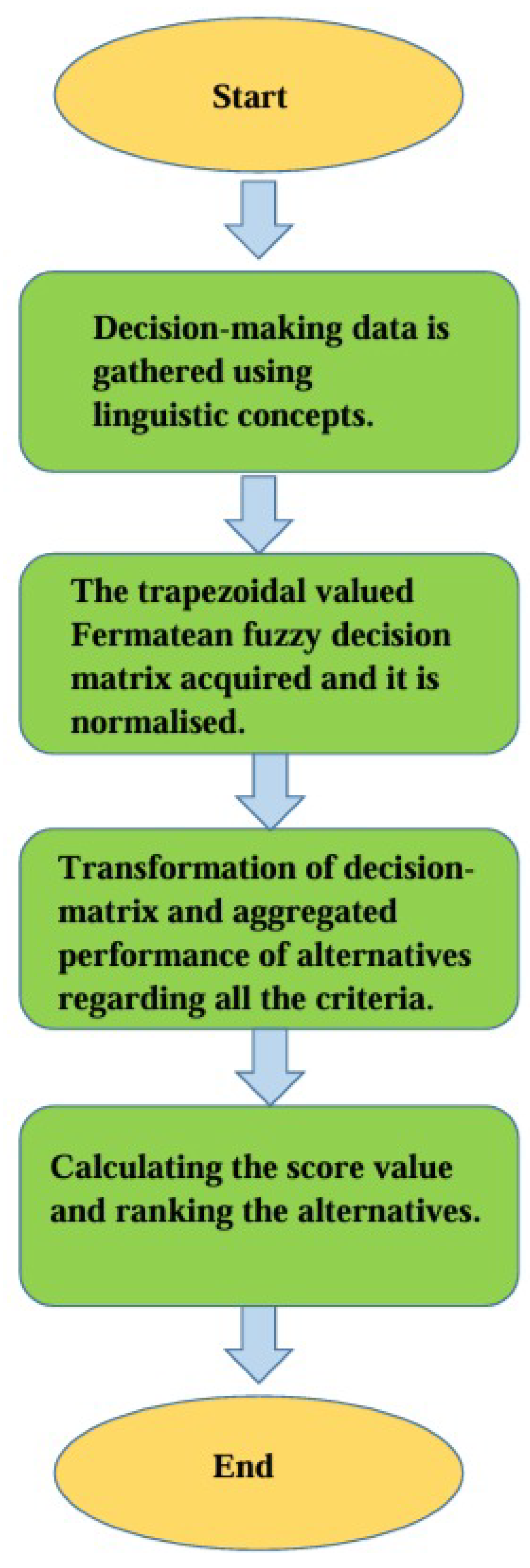
5. A Trapezoidal-Valued Fermatean Fuzzy Group Decision-Making Method

Through an elaborate procedure, this section develops a trapezoidal-valued multi-attribute choice-making algorithm. Let us look at the MAGDM problem, where A T p V 1 , A T p V 2 , …, and A T p V l are the alternatives and C t p 1 , C t p 2 , and C t p l are the attributes. Let E t p 1 , E t p 2 , and E t p l be experts with weights ω t p 1 , ω t p 1 , and ω t p l , respectively, where ω t p i 0 , i = 1 , 2 , l and i = 1 l ω t p i = 1 .
Step 1. Collection of Data: Decision-making data are gathered using linguistic concepts. Table 1 may be used to convert linguistic phrases into fermatean fuzzy integers with trapezoidal values and display them as a matrix for decision making. D = ( T p V i j ^ m × n ) , which also preserves symmetry in input weights and fuzzy evaluations, and every
T p V i j ^ = ( a i j Φ , b i j Φ , c i j Φ , d i j Φ ) , ( e i j Ψ , f i j Ψ , g i j Ψ , h i j Ψ )
Step 2. Normalisation of the fermatean fuzzy choice matrix using trapezoidal values: The TpVFF decision matrix D = ( T p V i j ^ m × n ) acquired in Step I is normalized to
D = ( T p V i j ^ ) m × n = ( a i j Φ , b i j Φ , c i j Φ , d i j Φ ) , ( e i j Ψ , f i j Ψ , g i j Ψ , h i j Ψ m × n
using the following equation.
( T p V i j ^ ) = ( a i j Φ , b i j Φ , c i j Φ , d i j Φ ) , ( e i j Ψ , f i j Ψ , g i j Ψ , h i j Ψ , i f i t i s a n a t t r i b u t e o f t h e b e n e f i t t y p e . ( e i j Ψ , f i j Ψ , g i j Ψ , h i j Ψ ) , ( a i j Φ , b i j Φ , r i j Φ , s i j Φ ) , i f i t i s a n a t t r i b u t e o f t h e c o s t t y p e .
In other words, the normalization indicates that
  • The membership value of ( T p V i j ^ ) is changed to a non-membership value ( T p V i j ^ ) , and the non-membership value is changed to ( T p V i j ^ ) , if the condition falls into the cost category.
  • T p V i j ^ = T p V i j ^ if the criteria are inside the benefit category. If every criterion taken into account for the problem is a benefit criterion, then this step can be omitted.
Step 3: Accumulated performance.
(a)
Transformation of decision matrix: This is carried out by the use of operators T p V F F D W G s. That is, T p V N D W G ( T p V 1 ^ , T p V 2 ^ , , T p V n ^ ) = i = 1 n ( T p V ^ i ) ω t p i
(b)
Aggregated performance of alternatives regarding all the criteria: This is derived by using the operator T p V F F D W G on every row of the combined matrix of decisions that was produced in Step 3(a).
Step 4: Score Matrix: Employ the scoring functions to obtain the score ( A T p V l ) for each alternative aggregated performance acquired in Step 3(b).
Step 5: Alternatives’ Ranking: According to the ranking concept, the options are ranked.

5.1. Problem Description

The primary goal of a pink cab, a specialist transportation service, is to improve women’s and children’s comfort, safety, and convenience. Social, safety, cultural, and economic issues all contribute to their necessity. In response to an increase in crimes against women in transport, pink taxis are being deployed in places like Delhi and Karachi. Women are frequently harassed, stalked, or put in dangerous circumstances when using public transportation or ordinary taxis in various places. By using female drivers and only carrying women and children, pink taxis provide a safer atmosphere. They frequently include emergency contact integration, GPS monitoring, and panic buttons.
  • Need for Pink Cabs
  • Safety: Defend women against abuse and harassment.
  • Cultural Appropriateness: Provide secure transportation in cultures that are sensitive to gender.
  • Emotional Comfort: Increase female passengers’ peace of mind.
  • Technological Security: Utilize GPS, apps, and panic buttons to improve mobility.
Example 1. The following are the five potential cities where pink taxi services might be introduced: A T p V 1 , A T p V 2 , A T p V 3 , A T p V 4 , and A T p V 5 . A panel of experts is formed E t p 1 (Urban Safety Analyst), E t p 2 (Gender Policy Expert), and E t p 3 (Transportation and Business Expert). Let us consider four criteria that are in conflict: C T p V 1 (Working Women’s Population) , C T p V 2 (Gaps in Public Transportation), C T p V 3 (Current Rate of Crime Against Women) , C T p V 4 (the price of launching). The weight vector of three experts ω t p 1 = 0.25 , ω t p 2 = 0.35 , a n d   ω t p 3 = 0.40 is 1. First, the experts will use linguistic ideas to generate a decision matrix. To show how the suggested M A G D M method may be used, we provide the following example:

5.2. Solving the Proposed Trapezoidal-Valued Fermetean Fuzzy MAGDM

First, we use the proposed T p V F F M A G D M method to analyze Example 1 and Figure 1.
Step 1. Data Collection: Three experts were consulted, and they evaluated the performance of five options using four criteria. Then, using Table 1, the linguistic terms extracted from the panel’s data were converted into T p V F F N . As shown in Table 2, we obtained regarding Expert 1’s Criterion 1: the linguistic term for Alternative 1 as “D” after compiling the data from each expert. Consequently, the T p V F F N was used in place of the linguistic word, “D”, with ( 0.51 , 0.49 , 0.66 , 0.69 ) , ( 0.41 , 0.48 , 0.52 , 0.27 ) . Table 1 provides the definitions of used terms.
Step 2. Normalization: No normalization process is necessary in this case because all of the criteria are benefit-type.
Step 3: Accumulated Decision Matrix: Table 3 shows the cumulative choice matrix that is produced at this step. Take Table 2 as an example.
  • We obtain ( 0.793 , 0.778 , 0.882 , 0.896 ) , ( 0.644 , 0.512 , 0.444 , 0.891 ) by using the formula for T p V F F N from Theorem 2. We can calculate each other entry in Table 3 in a similar way. We add up the values of each criterion with regard to Table 4.
Step 4. Score Values: The overall effectiveness of the four solutions in relation to the four criteria is displayed in Table 4’s second column. By applying the scoring function, we can obtain the score value for each option. The following are the final scores for the four options: A T p V 1 = 0.382 , A T p V 2 = 0.409 , A T p V 3 = 0.474 , A T p V 4 = 0.369 , and A T p V 5 = 0.319 .
Step 5. Alternatives’ ranking: According to the ranking concept, the options are ranked and graphically represented in Figure 2. A T p V 3 > A T p V 2 > A T p V 1 > A T p V 4 > A T p V 5
Thus, first, A T p V 3 city is needed for the introduction of pink taxi services.

5.3. Comparative Analysis

Example 2. Let us look at an MAGDM issue with three criteria, C T p V 1 , C T p V 2 and C T p V 3 , and three alternatives, A T p V 1 , A T p V 2 and A T p V 3 (Table 5).
The weights of the three criteria, C T p V 1 , C T p V 2 and C T p V 3 , will now be assumed to be 0.25, 0.35, and 0.40, respectively. Here, we evaluate our MAGDM approach against various methods; the outcome is displayed in Table 6 below.

5.4. Advantages of the Suggested MAGDM Strategy

We outline a few benefits of our suggested MAGDM approach in this paragraph:
  • First, the comprehensive ordering concept on TpVFFNs—which encompasses TFFNs, FFNs, and IVFFNs under a broad heading—is used in our suggested MAGDM strategy. Consequently, the following issues might be resolved using the suggested strategy in the subclass context: real-valued FFNs, IVFFNs, and TFFNs.
  • The MAGDM algorithm integrates the full-ordering principle; therefore, our proposed method may always rank the two unique TpVFFNs. In other words, two different options will never be ranked by the suggested MAGDM technique (different performances according to independent criteria) as equal.
  • Thirdly, by altering the Dombi variable, D t n - and D t c n -oriented aggregating operators have the benefit of making the aggregating process simpler. Flexibility may be achieved by altering the Dombi operator’s variable. Its adjustable parameters make it more adaptable than other t-norms and t-conorms currently in use. By altering the variable’s Dombi accumulation operator value, we may vary the norm that is applied to accumulation, which also alters the operational behavior of the parameter.

6. Sensitive Analysis

In fuzzy aggregation procedures, the Dombi parameter γ T p V is essential because it regulates the ratio of flexibility to strictness in the decision-making process. This parameter is especially significant when discussing T p V F F N s since it enables the aggregation behavior to represent a range of decision makers’ attitudes, from extremely optimistic to conservative, or risk-averse. The Dombi operator adds an adjustable parameter that modifies the operation’s sharpness, in contrast to fixed aggregation operators like the algebraic or Einstein t-norms. For optimistic or neutral decision contexts, lower values of T p V F F N s tend to yield smoother, more average-like results. Higher values of T p V F F N s, on the other hand, cause the operator to act more like a minimal or maximum function, which is consistent with more cautious or optimist inclinations. Because of this adaptability, decision makers may alter the model to fit their preferred aggregate strictness and risk profiles. This investigation will show that while the alternatives’ absolute score values somewhat declined as the values of TpV increased, the alternatives’ overall ranking stayed constant. This implies that considerable resilience against moderate alterations in the Dombi parameter is exhibited by the suggested TpVFFN-based model. Because it shows that slight variations in aggregate preference do not result in significant changes to the final recommendations, this stability is useful in decision-making systems. Overall, this sensitivity study demonstrates the Dombi-based TpVFFN model’s versatility and resilience. Different risk attitudes can be reflected in the model without sacrificing the consistency of the decision-making process by adjusting TpV. This characteristic is particularly useful in real-world multi-attribute issues where decision makers may have different risk and ambiguity tolerance levels and where subjectivity and uncertainty are prevalent. Even though this study used a constant value for γ T p V , future research might benefit from examining how changes in this parameter impact decision results.

7. Conclusions

In this paper, we used TpVFFs to examine decision-making difficulties. We suggested three new accumulation operators—TpVFFDWG, TpVFFDOWG, and TpVFFDHG—to manage the aggregation of TpVFFNs. Fundamental theorems were used to validate and thoroughly investigate the theoretical underpinnings and important characteristics of these operators. Additionally, we included these suggested operators into a novel TpVFFMAGDM method, with the suggested TpVFFN-based aggregation architecture ensuring symmetry. Using these operators as a foundation, we created a novel TpVFFMAGDM method specifically designed for the deployment scenario of pink taxis. Through a real-world case study, the efficacy of the suggested approach was illustrated, emphasizing its capacity to handle intricate, contradictory criteria and ambiguity in expert evaluations during city selection.
Future studies can apply the idea of TpVFFNs to more complicated and dynamic decision-making settings, such as adaptive and real-time systems. The practical value of TpVFFNs might be improved by a further development of sophisticated aggregation operators, integration with intelligent systems like machine learning models, and applications in cutting-edge domains—including smart cities, healthcare analytics, and sustainable development. Furthermore, the model’s dependability and acceptance in practical situations would be reinforced by integrating TpVFFN-based frameworks into decision-support software and by carrying out exhaustive sensitivity and robustness evaluations.

Author Contributions

Conceptualization, M.K. and J.A.; methodology, M.K.; software, J.A.; validation, M.K., J.A. and M.A.; formal analysis, M.A.; investigation, M.A.; resources, M.A.; data curation, J.A.; writing—original draft preparation, M.K.; writing—review and editing, M.K.; supervision, M.A.; project administration, M.A. All authors have read and agreed to the published version of the manuscript.

Funding

This research received no external funding.

Data Availability Statement

No new data were created or analyzed in this study. Data sharing is not applicable to this article.

Conflicts of Interest

The authors declare no conflicts of interest.

References

  1. Zadeh, L.A. Fuzzy sets. Inf. Control 1965, 8, 338–353. [Google Scholar] [CrossRef]
  2. Atanassov, K.T. Intuitionistic fuzzy sets. Fuzzy Sets Syst. 1986, 20, 87–96. [Google Scholar] [CrossRef]
  3. Smarandache, F. A Unifying Field in Logics. Neutrosophy: Neutrosophic Probability, Set and Logic; American Research Press: Rehoboth, DE, USA, 1999. [Google Scholar]
  4. Ye, J. An extended TOPSIS method for multiple attribute group decision making based on single valued neutrosophic linguistic numbers. J. Intell. Fuzzy Syst. 2015, 28, 247–255. [Google Scholar] [CrossRef]
  5. Chi, P.; Liu, P. An extended TOPSIS method for the multiple attribute decision making problems based on interval neutrosophic set. Neutrosophic Sets Syst. 2013, 1, 63–70. [Google Scholar]
  6. Bui, Q.-T.; Ngo, M.-P.; Snasel, V.; Pedrycz, W.; Vo, B. Information measures based on similarity under neutrosophic fuzzy environment and multi-criteria decision problems. Eng. Appl. Artif. Intell. 2023, 122, 106026. [Google Scholar] [CrossRef]
  7. Ali, M.; Hussain, Z.; Yang, M.-S. Hausdorff distance and similarity measures for single-valued neutrosophic sets with application in multi-criteria decision making. Electronics 2022, 12, 201. [Google Scholar] [CrossRef]
  8. Dombi, J. A general class of fuzzy operators, the DeMorgan class of fuzzy operators and fuzziness measures induced by fuzzy operators. Fuzzy Sets Syst. 1982, 8, 149–163. [Google Scholar] [CrossRef]
  9. Liu, P.; Liu, J.; Chen, S.-M. Some intuitionistic fuzzy Dombi Bonferroni mean operators and their application to multi-attribute group decision making. J. Oper. Res. Soc. 2018, 69, 1–24. [Google Scholar] [CrossRef]
  10. Seikh, M.R.; Mandal, U. Intuitionistic fuzzy Dombi accumulation Operators and their application to multiple attribute decision-making. Granul. Comput. 2021, 6, 473–488. [Google Scholar] [CrossRef]
  11. Shi, L.; Ye, J. Dombi Aggregation Operators of Neutrosophic Cubic Sets for Multiple Attribute Decision-Making. Algorithms 2018, 11, 29. [Google Scholar] [CrossRef]
  12. Shao, Y.; Zhuo, J. Improved q-rung orthopair fuzzy line integral accumulation Operators and their applications for multiple attribute decision making. Artif. Intell. Rev. 2021, 54, 5163–5204. [Google Scholar] [CrossRef]
  13. Deveci, M.; Gokasar, I.; Castillo, O.; Daim, T. Evaluation of metaverse integration of freight fluidity measurement alternatives using fuzzy Dombi EDAS model. Comput. Ind. Eng. 2022, 174, 108773. [Google Scholar] [CrossRef]
  14. Jana, C.; Senapati, T.; Pal, M.; Yager, R.R. Picture fuzzy Dombi accumulation Operators: Application to MADM process. Appl. Soft Comput. 2019, 74, 99–109. [Google Scholar] [CrossRef]
  15. Kumar, R.; Pamucar, D. A comprehensive and systematic review of MCDM (MCDM) methods to solve decision-making problems: Two decades from 2004 to 2024. Spectr. Decis. Mak. Appl. 2025, 2, 178–197. [Google Scholar] [CrossRef]
  16. Ali, A.; Ullah, K.; Hussain, A. An approach to multi-attribute decision-making based on intuitionistic fuzzy soft information and Aczel-Alsina operational laws. J. Decis. Anal. Intell. Comput. 2023, 3, 80–89. [Google Scholar] [CrossRef]
  17. Asif, M.; Ishtiaq, U.; Argyros, I.K. Hamacher accumulation Operators for Pythagorean fuzzy set and its application in multi-attribute decision-making problem. Spectr. Oper. Res. 2025, 2, 27–40. [Google Scholar] [CrossRef]
  18. Sahoo, S.K.; Pamucar, D.; Goswami, S.S. A review of MCDM applications to solve energy management problems from 2010–2025: Current state and future research. Spectr. Decis. Mak. Appl. 2025, 2, 219–241. [Google Scholar] [CrossRef]
  19. Naeem, M.; Ali, J. A novel multi-criteria group decision-making method based on Aczel-Alsina spherical fuzzy accumulation operators: Application to evaluation of solar energy cells. Phys. Scr. 2022, 97, 085203. [Google Scholar] [CrossRef]
  20. Khatter, K. Interval valued trapezoidal neutrosophic set: Multi-attribute decision making for prioritization of non-functional requirements. J. Ambient. Intell. Humaniz. Comput. 2021, 12, 1039–1055. [Google Scholar] [CrossRef]
  21. Nayagam, V.L.; Jeevaraj, S.; Dhanasekaran, P. An improved ranking method for comparing trapezoidal intuitionistic fuzzy numbers and its applications to multicriteria decision making. Neural Comput. Appl. 2018, 30, 671–682. [Google Scholar] [CrossRef]
  22. Meher, B.B.; Jeevaraj, S.; Alrasheedi, M. Dombi weighted geometric aggregation operators on the class of trapezoidal-valued intuitionistic fuzzy numbers and their applications to multi-attribute group decision-making. Artif. Intell. Rev. 2025, 58, 205. [Google Scholar] [CrossRef]
  23. Bihari, R.; Jeevaraj, S.; Kumar, A. A new ranking principle for ordering generalized trapezoidal fuzzy numbers based on diagonal distance, mean and its applications to supplier selection. Soft Comput. 2023. [Google Scholar] [CrossRef]
  24. Senapati, T.; Yager, R.R. Some new operations over Fermatean fuzzy numbers and application of Fermatean fuzzy WPM in multiple criteria decision making. Informatica 2019, 30, 391–412. [Google Scholar] [CrossRef]
  25. Mishra, A.R.; Rani, P. Multi-criteria healthcare waste disposal location selection based on Fermatean fuzzy WASPAS method. Complex Intell. Syst. 2021, 7, 2469–2484. [Google Scholar] [CrossRef]
  26. Garg, H.; Shahzadi, G.; Akram, M. Decision-making analysis based on Fermatean fuzzy Yager aggregation operators with application in COVID-19 testing facility. Math. Probl. Eng. 2020, 2020, 7279027. [Google Scholar] [CrossRef]
  27. Yang, Z.; Garg, H.; Li, X. Differential calculus of Fermatean fuzzy functions: Continuities, derivatives, and differentials. Int. J. Comput. Intell. Syst. 2021, 14, 282–294. [Google Scholar] [CrossRef]
  28. Sergi, D.; Sari, I.U. Fuzzy capital budgeting using Fermatean fuzzy sets. In Proceedings of the International Conference on Intelligent and Fuzzy Systems, Istanbul, Turkey, 21–23 July 2020; pp. 448–456. [Google Scholar]
  29. Sahoo, L. Some score functions on Fermatean fuzzy sets and its application to bride selection based on TOPSIS method. Int. J. Fuzzy Syst. Appl. 2021, 10, 18–29. [Google Scholar] [CrossRef]
  30. Wu, L.; Wei, G.; Gao, H.; Wei, Y. Some interval-valued intuitionistic fuzzy Dombi Hamy mean operators and their application for evaluating the elderly tourism service quality in tourism destination. Mathematics 2018, 6, 294. [Google Scholar] [CrossRef]
  31. Lu, S.; Cheng, L. Pure rational and non-pure rational decision methods on interval-valued fuzzy soft β-covering approximation spaces. Expert Syst. Appl. 2025, 288, 128262. [Google Scholar] [CrossRef]
  32. Torra, V. Hesitant fuzzy sets. Int. J. Intell. Syst. 2010, 25, 529–539. [Google Scholar] [CrossRef]
  33. Lu, S.; Xu, Z.; Fu, Z.; Cheng, L.; Yang, T. Foundational theories of hesitant fuzzy sets and hesitant fuzzy information systems and their applications for multi-strength intelligent classifiers. Inf. Sci. 2025, 714, 122212. [Google Scholar] [CrossRef]
  34. Senapati, T.; Chen, G.; Mesiar, R.; Yager, R.R. Novel Aczel–Alsina operations-based interval-valued intuitionistic fuzzy aggregation operators and their applications in multiple attribute decision-making process. Int. J. Intell. Syst. 2022, 37, 5059–5081. [Google Scholar] [CrossRef]
  35. Senapati, T.; Mesiar, R.; Simic, V.; Iampan, A.; Chinram, R.; Ali, R. Analysis of interval-valued intuitionistic fuzzy Aczel–Alsina geometric aggregation operators and their application to multiple attribute decision-making. Axioms 2022, 11, 258. [Google Scholar] [CrossRef]
Figure 1. Flowchart for the proposed T p V F F M A G D M method.
Symmetry 17 01114 g001
Figure 2. Alternatives final ranking using score values.
Symmetry 17 01114 g002
Table 1. Linguistic value.
Linguistic Variables TpVFFN s
VD (Very Dissatisfied)(0.32,0.45,0.35,0.43), (0.21,0.33,0.42,0.52)
D (Dissatisfied)(0.51,0.49,0.66,0.69), (0.41,0.48,0.52,0.27)
N (Neutral)(0.62,0.69,0.55,0.65), (0.63,0.59,0.71,0.49)
S (Satisfied)(0.74,0.67,0.59,0.51), (0.61,0.52,0.63,0.71)
VS (Very Satisfied)(0.61,0.80,0.72,0.59), (0.89,0.40,0.56,0.70)
Table 2. Linguistic multi-attribute.
ExpertsAlternativesAttribute
C T pV 1 C T pV 2 C T pV 3 C T pV 4 .
E t p 1 A T p V 1 DVS.VDS
A T p V 2 NSDVS.
A T p V 3 VS.DVS.N
A T p V 4 VDVS.ND
A T p V 5 SNVSVD
E t p 2 A T p V 1 DVDNS
A T p V 2 SNVDD
A T p V 3 VSDNVD
A T p V 4 NSVS.D
A T p V 5 VDNSVS.
E t p 3 A T z V 1 DNSVS.
A T p V 2 VS.VDND
A T p V 3 SDVS.VD
A T p V 4 NSVDVS.
A T p V 5 SVS.DN
Table 3. Decision matrix.
AlternativeAttribute ( C T p V 1 )
A T p V 1 (0.793,0.778,0.882,0.896), (0.644,0.512,0.444,0.891)
A T p V 2 (0.863,0.897,0.827,0.869), (0.242,0.587,0.339,0.292)
A T p V 3 (0.859,0.939,0.897,0.839), (0.254,0.583,0.341,0.207)
A T p V 4 (0.651,0.764,0.678,0.749), (0.772,0.522,0.358,0.489)
A T p V 5 (0.837,0.873,0.805,0.785), (0.886,0.666,0.485,0.335)
AlternativeAttribute ( C T p V 2 )
A T p V 1 (0.795,0.950,0.849,0.833), (0.886,0.671,0.480,0.459)
A T p V 2 (0.805,0.866,0.787,0.785), (0.918,0.671,0.529,0.449)
A T p V 3 (0.793,0.778,0.882,0.896), (0.644,0.512,0.444,0.891)
A T p V 4 (0.861,0.937,0.903,0.835), (0.300,0.493,0.305,0.203)
A T p V 5 (0.861,0.897,0.825,0.875), (0.227,0.575,0.323,0.404)
AlternativeAttribute ( C T p V 3 )
A T p V 1 (0.652,0.764,0.679,0.7444), (0.772,0.546,0.377,0.442)
A T p V 2 (0.759,0.782,0.830,0.876), (0.888,0.658,0.485,0.664)
A T p V 3 (0.857,0.939,0.905,0.847), (0.206,0.604,0.341,0.372)
A T p V 4 (0.773,0.874,0.773,0.850), (0.917,0.740,0.542,0.405)
A T p V 5 (0.851,0.921,0.898,0.844), (0.551,0.523,0.396,0.823)
AlternativeAttribute ( C T p V 4 )
A T p V 1 (0.914,0.889,0.848,0.798), (0.247,0.592,0.345,0.207)
A T p V 2 (0.845,0.911,0.908,0.850), (0.622,0.541,0.437,0.878)
A T p V 3 (0.731,0.860,0.743,0.836), (0.947,0.779,0.603,0.451)
A T p V 4 (0.798,0.787,0.883,0.889), (0.529,0.608,0.415,0.812)
A T p V 5 (0.651,0.765,0.680,0.747), (0.770,0.611,0.396,0.432)
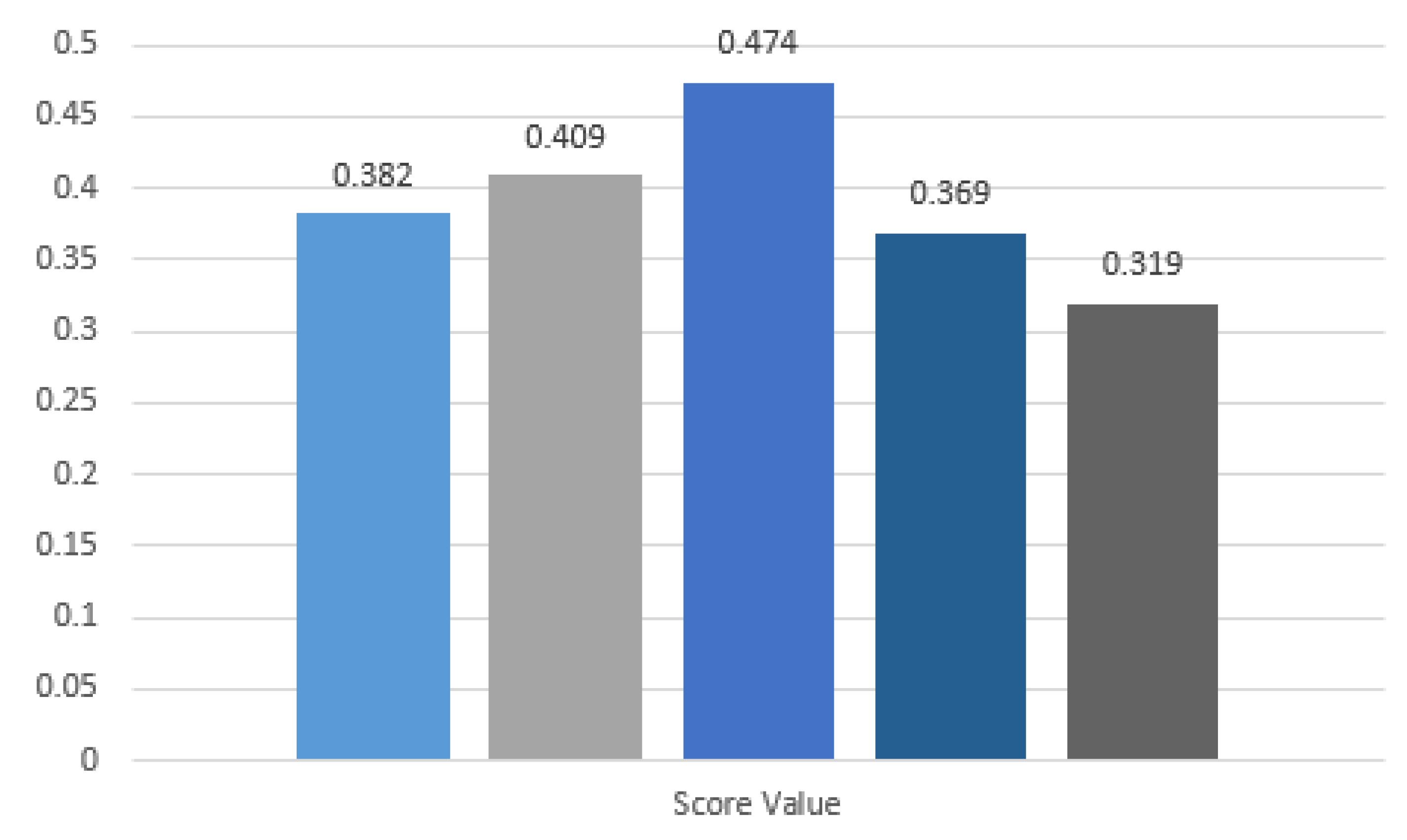
Table 4. Score values.
AlternativeFinal ValueScore Value
A T p V 1 (0.788,0.845,0.814,0.817), (0.637,0.580,0.411,0.499)0.382
A T p V 2 (0.818,0.864,0.838,0.845), (0.667,0.614,0.447,0.570)0.409
A T p V 3 (0.810,0.879,0.856,0.854), (0.512,0.619,0.432,0.480)0.474
A T p V 4 (0.770,0.840,0.785,0.830), (0.629,0.590,0.405,0.477)0.369
A T p V 5 (0.8,0.864,0.802,0.812), (0.812,0.593,0.4,0.498)0.319
Table 5. Decision matrix.
C T pV 1 C T pV 2 C T pV 3
A T p V 1 (0.62,0.69), (0.63,0.59)(0.74,0.67), (0.61,0.52)(0.51,0.49), (0.41,0.48)
A T p V 2 (0.74,0.67), (0.63,0.71)(0.62,0.69), (0.71,0.49)(0.32,0.45), (0.42,0.52)
A T p V 3 (0.72,0.59), (0.56,0.70)(0.35,0.43), (0.42,0.52)(0.55,0.65), (0.71,0.49)
Table 6. Comparative analysis.
Operator A T pV 1 A T pV 2 A T pV 3 Ranking OrderIdeal Ranking
Wu et al. [30] (IVIFWDHM)0.3690.3590.272 A T p V 1 > A T p V 2 > A T p V 3 A T p V 1
Senapati et al. [34] (IVIFAAWA)0.4950.4810.338 A T p V 1 > A T p V 2 > A T p V 3 A T p V 1
Senapati et al. [35] (IVIFAAWG)0.4850.4780.332 A T p V 1 > A T p V 2 > A T p V 3 A T p V 1
Meher et al. [22] (TrVIFDWG)0.6930.6780.611 A T p V 1 > A T p V 2 > A T p V 3 A T p V 1
Proposed ( T p V F F D W G ) 0.5640.4660.418 A T p V 1 > A T p V 2 > A T p V 3 A T p V 1
Disclaimer/Publisher’s Note: The statements, opinions and data contained in all publications are solely those of the individual author(s) and contributor(s) and not of MDPI and/or the editor(s). MDPI and/or the editor(s) disclaim responsibility for any injury to people or property resulting from any ideas, methods, instructions or products referred to in the content.

