A Novel Heterogeneous Federated Edge Learning Framework Empowered with SWIPT

Abstract

Federated edge learning (FEEL) is an innovative approach that facilitates collaborative training among numerous distributed edge devices while eliminating the need to transfer sensitive information. However, the practical deployment of FEEL faces significant constraints, owing to the limited and asymmetric computational and communication resources of these devices, along with their energy availability. To this end, we propose a novel asymmetry-tolerant training approach for FEEL, enabled via simultaneous wireless information and power transfer (SWIPT). This framework leverages SWIPT to offer sustainable energy support for devices while enabling them to train models with varying intensities. Given a limited energy budget, we highlight the critical trade-off between heterogeneous local training intensities and the quality of wireless transmission, suggesting that the design of local training and wireless transmission should be closely integrated, rather than treated as separate entities. To elucidate this perspective, we rigorously derive a new explicit upper bound that captures the combined impact of local training accuracy and the mean square error of wireless aggregation on the convergence performance of FEEL. To maximize overall system performance, we formulate two key optimization problems: the first aims to maximize the energy harvesting capability among all devices, while the second addresses the joint learning–communication optimization under the optimal energy harvesting solution. Comprehensive experiments demonstrate that our proposed framework achieves significant performance improvements compared to existing baselines.

1. Introduction

The rapid development of the Sixth Generation Wireless Communication System will enhance the interconnection of intelligent agents, facilitating the shift from the “Internet of Everything” to “Intelligent Connectivity of Everything” within the Internet of Things (IoT) framework. Consequently, a diverse array of device terminals and data will continuously emerge, making it crucial to ensure low latency and high reliability in data processing while achieving flexible and privacy-preserving network interconnection. To confront these challenges, federated edge learning (FEEL) has arisen as a promising paradigm in edge learning, thanks to its strong capabilities in data privacy protection and efficient utilization of terminal computational resources. The FEEL framework allows terminal devices to leverage local data for the autonomous training of machine learning models, transmitting only the trained models to the base station (BS) via wireless networks without revealing local private data [1,2,3]. However, as wireless resources become scarcer and the influx of IoT devices increases, the issue of learning efficiency in FEEL systems has gained prominence, highlighting the need for further research and solutions.

1.1. State-of-the-Art

In existing research, the primary approaches to enhancing the efficiency of the FEEL framework focus on improving local computation efficiency and wireless transmission quality. Among these, optimizing local computation methods aims to enhance resource utilization, achieving faster training speeds and a lower communication overhead. One of the seminal approaches to improving local computational efficiency in FEEL is the communication-efficient federated averaging (FedAvg) algorithm [4,5]. This algorithm enables edge devices to undertake multiple iterations of local model updates, thereby yielding a more refined gradient descent direction. Consequently, FedAvg effectively diminishes the frequency of global communication, serving as a quintessential embodiment of the “trade computation for communication” strategy. Nonetheless, this learning paradigm relies on synchronous aggregation, requiring all devices to undergo the same number of local training iterations. This “one-size-fits-all” methodology inadequately leverages the computational capabilities inherent to each device, particularly in future large-scale IoT ecosystems, where significant asymmetries in processing power, storage capacity, and energy availability among edge devices are expected [6]. Although several studies have proposed asynchronous or semi-asynchronous FEEL training frameworks, e.g., [7,8,9,10], to mitigate this limitation, these mechanisms often lead to increased communication frequency between the BS and edge devices. Concurrently, the irregular update frequency from slower devices can lead to significant staleness in their local models relative to the global model [11]. In this context, a more effective strategy involves the dynamic allocation of training intensity based on the computational capabilities of each device, e.g., employing lower training intensities for less capable devices while reserving higher intensities for those with greater capabilities. For instance, several studies, e.g., [12,13,14,15,16], have proposed a series of asymmetry-tolerant FEEL frameworks that dynamically assign different training intensities (e.g., the number of local updates, batch size, or network blocks) to mitigate waiting delays. Within these frameworks, local training intensity is primarily governed by the maximum permissible delay and the inherent computational capabilities of the devices, with increased local training intensity often viewed as a mechanism to accelerate convergence.

Conversely, enhancing the quality of wireless transmission primarily seeks to mitigate inherent characteristics of wireless communication, including channel fading, noise interference, and multipath effects [17]. These factors may introduce substantial perturbation errors in model parameters during transmission, which can accumulate during the global model aggregation and update processes. In response, several wireless implementation solutions have been proposed to facilitate the operation of the FEEL framework. According to the existing research, the predominant communication protocols for the transmission of FEEL models primarily include Orthogonal Multiple Access (OMA) [18,19,20] and over-the-air computation (AirComp) [21,22,23]. OMA achieves signal separation by allocating independent time or frequency resources to different devices, effectively mitigating inter-device interference and thus enhancing overall system capacity. In contrast to the resource separation strategy employed by OMA, AirComp leverages the superposition characteristics of electromagnetic waves propagating through free space. This approach enables the direct aggregation of distributed data transmitted synchronously between devices, eliminating the need to decode the data at the BS before computation. For instance, the work in [21] presented an accelerated global model aggregation approach that leverages AirComp, formulating a sparse low-rank optimization problem to jointly design device selection strategies alongside beamforming schemes. An extended version of this work, detailed in [22], namely one-bit over-the-air computation, utilizes a truncated-channel-inversion power control strategy to implement an innovative digital approach for broadband AirComp aggregation. Additionally, the research in [23] tackled the challenge of minimizing training latency and energy consumption in scenarios where devices continuously collect new data. In this context, an average training error metric is proposed to evaluate convergence performance, along with a resource allocation strategy developed using deep reinforcement learning techniques.

1.2. Motivations and Contributions

As shown in

Table 1. Comparisons of this work with other representative works.

Ref.	FEEL Scenario?	Heterogeneity Consideration?	Communication-Learning Design?	SWIPT?
[4,5]	✓
[7,8,9,10,12,13,14,15,16]	✓	✓
[18,19,20,21,22,23]	✓		✓
[24,25,26,27]				✓
This Work	✓	✓	✓	✓

If a work has a check mark in a column, it indicates that the work meets the specific criteria listed at the top of that column.

, we list the specific research content of some state-of-the-art works. Judging from the existing literature, most studies treat the design of local training intensity and wireless transmission strategies as two separate issues. However, we recognize that there may be a trade-off between local training and wireless communication. The underlying logic is that edge devices typically have a limited battery capacity (as seen in sensors), and this capacity must support both local training tasks and the transmission of model updates in uncontrollable wireless environments. In such cases, solely optimizing computation or wireless transmission strategies often leads the system to face a dilemma: if devices prioritize computation and allocate most of their energy to local training, they may lack sufficient residual energy to sustain wireless communication, resulting in more severe transmission distortions. Conversely, if they excessively reduce local training intensity to ensure wireless transmission quality, they may fail to maintain adequate model update quality, hindering the achievement of the desired global convergence accuracy. Against this backdrop, this paper makes efforts in two main areas. First, we consider applying simultaneous wireless information and power transfer (SWIPT) during the training process to provide wireless energy to these energy-constrained devices, thereby alleviating issues of inadequate training or wireless distortion caused by insufficient energy. The primary benefit of SWIPT is its ability to facilitate concurrent data transmission while also enabling wireless power transfer [24,25,26,27]. For example, the work in [26] proposed a integration technique that combines SWIPT, single-input–multiple-output, and non-orthogonal multiple access to enhance device connectivity and power supply for cell-edge sensors while also improving outage performance through a transmit antenna selection strategy for the base station. In [27], the authors proposed leveraging a hybrid approach that combines time-switching and power-splitting energy at the relay user equipment to minimize the outage probability as much as possible. The aforementioned studies validate the notion that SWIPT is particularly well suited to services that are both energy-intensive and latency-sensitive, which motivates us to apply it to FEEL. Second, under the constraints of limited energy budgets, we precisely characterize the synergistic impact of local training and wireless transmission on the overall performance of the system from a global perspective and design a joint optimization strategy that takes both into account. The key contributions of this paper can be outlined as follows:

• We propose a SWIPT-enabled, asymmetry-tolerance training mechanism for FEEL with two key objectives: (1) alleviating the negative impact of device asymmetry through flexible training intensity and (2) utilizing SWIPT to mitigate training insufficiencies and wireless distortion issues arising from battery limitations, thus enabling FEEL applications on low-end devices. In this context, we acknowledge that, when edge devices operate under limited energy budgets, a critical trade-off may exist between heterogeneous local training intensity and wireless transmission quality. This indicates that local training intensity and wireless transmission strategies should be closely integrated, rather than entirely decoupled.
• To clarify this potential trade-off, we systematically derive the impact of device heterogeneous local training intensity and AirComp aggregation errors on the upper bound of FEEL convergence performance, theoretically revealing the key role of balancing training and transmission under energy-constrained conditions for system convergence efficiency. Our theoretical findings suggest that naively increasing local training intensity under limited energy budgets may inadvertently degrade final training performance. This contrasts with existing research, e.g., [5,12], which often views increasing local training intensity as an effective way to accelerate convergence without considering wireless aggregation distortion issues.
• To maximize system performance, we identify two critical optimization problems. The first problem is a SWIPT optimization problem aimed at maximizing the harvested power across all devices while ensuring successful decoding of global model information. The second problem is a joint learning–communication optimization problem that operates within the available energy of devices, guiding the joint design of uplink transmit beamforming for both devices and the BS, along with local training intensity. To tackle the non-convexity of these optimization problems, we propose an efficient alternating optimization (AO) strategy that combines successive convex approximation (SCA) with first-order Taylor expansion. The simulation results show that the proposed SWIPT-enabled FEEL heterogeneous training mechanism significantly enhances learning performance compared to baseline solutions.

The structure of this paper is laid out concisely as follows. Section 2 outlines the relevant learning and communication strategies. In Section 3, we provide a theoretical analysis of the convergence performance of our system and formulate the problem of maximizing learning performance. Section 4 introduces an AO algorithm designed to jointly optimize the SWIPT optimization problem and the joint learning–communication optimization problem. Section 5 discusses the numerical experiments conducted, and finally, our conclusions are presented in Section 6.

2. System Model

In this section, we outline the underlying learning framework and communication model.

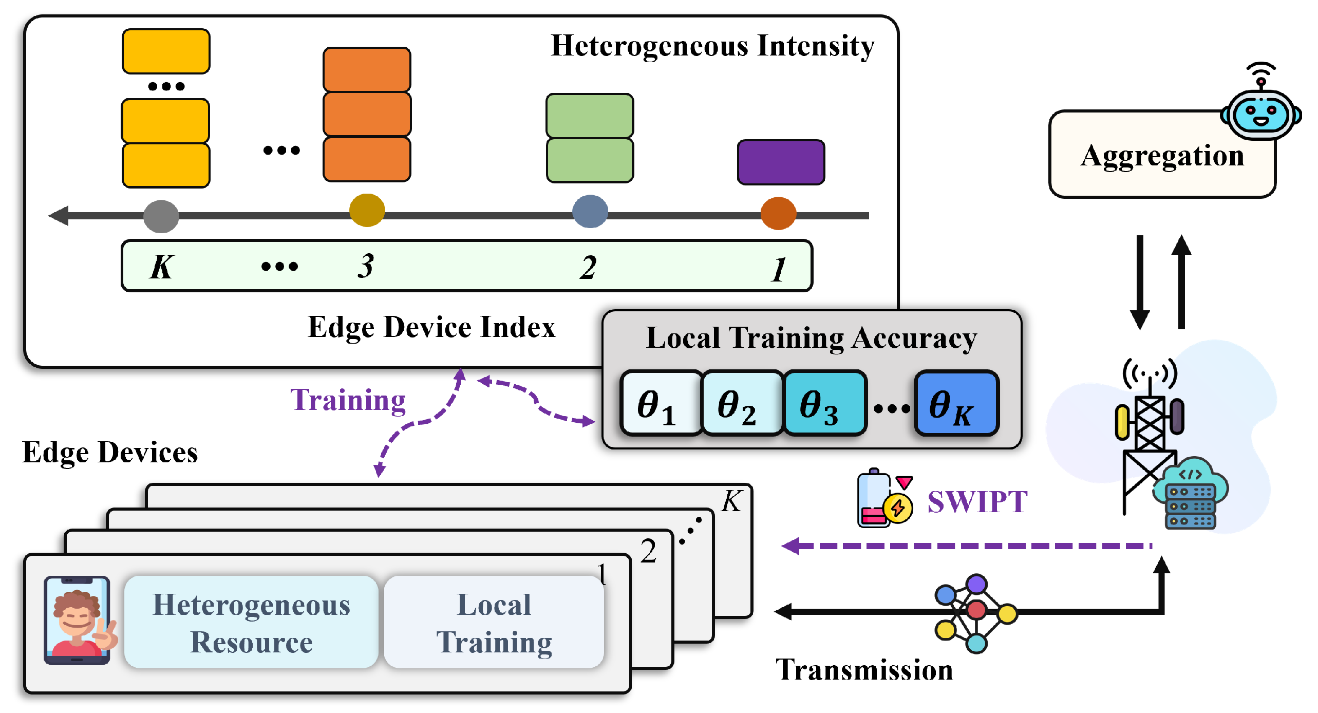
2.1. Federated Learning Framework

As illustrated in Figure 1, we consider a standard FEEL system that involves a collection of distributed edge devices, denoted by the index set $\mathcal{K}\triangleq \left\{1,2,\dots ,K\right\}$. These devices are orchestrated via a BS to collaboratively develop a global model ${\mathbf{w}}^{*}\in {\mathbb{R}}^D$ using their local datasets ${\mathcal{D}}_k$, by tackling the problem of

$$\underset{\mathbf{w}}{min}F\left(\mathbf{w}\right)\triangleq {\displaystyle \frac{1}{K}}\sum _{k\in \mathcal{K}}{F}_k\left(\mathbf{w}\right).$$

(1)

Here, $F_k\left(\mathbf{w}\right)$ is expressed as

$$F_k\left(\mathbf{w}\right)\triangleq {\displaystyle \frac{1}{\left|{\mathcal{D}}_k\right|}}\sum _{i=1}^{\left|{\mathcal{D}}_k\right|}f\left(\mathbf{w},{\mathbf{x}}_i,y_i\right),\forall k\in \mathcal{K},$$

(2)

where $\left|{\mathcal{D}}_k\right|$ indicates the total number of samples in device k’s local dataset, and $f(\mathbf{w},{\mathbf{x}}_i,y_i)$ represents the prediction error of model $\mathbf{w}$ on the input feature vector ${\mathbf{x}}_i$ compared to its true label $y_i$.

We assume in this paper that edge devices utilize the stochastic average gradient (SAG) algorithm [5,6] for local training. Let the complete training process last for N iterations. Then, during iteration n, where $1\le n\le N$, the interaction process between devices and the BS can be summarized as

• Downlink model broadcast: The BS broadcasts the feedback information to all devices using SWIPT, which includes the global model parameters from the previous iteration ${\mathbf{w}}^{n-1}$ and the aggregated gradient $\nabla {\tilde{\mathbf{F}}}^{n-1}$ (as defined in Equations (5) and (6)). Subsequently, each device, integrated with a power splitter [28], receives the global parameters along with radio frequency energy from the BS.
• Heterogeneous local computation: Each device performs local training based on the following surrogate objective function:

  $$\underset{\mathbf{w}\in {\mathbb{R}}^D}{min}{J}_k^n\left(\mathbf{w}\right)\triangleq F_k\left(\mathbf{w}\right)+〈\eta \nabla {\tilde{\mathbf{F}}}^{n-1}-\nabla F_k\left({\mathbf{w}}^{n-1}\right),\mathbf{w}〉.$$

  (3)
  It can be observed that $J_k^n\left(\mathbf{w}\right)$ dynamically adjusts the optimization objective by incorporating $\nabla {\tilde{\mathbf{F}}}^{n-1}$ and $\nabla F_k\left({\mathbf{w}}^{n-1}\right)$ into $F_k\left(\mathbf{w}\right)$, thereby better aligning with the convergence requirements of the global optimization process [5]. Considering the limitations of device computing capabilities in practical resource-constrained FEEL environments, this paper introduces an approximate solving strategy to achieve a reasonable balance between computational complexity and model training effectiveness. Specifically, each device obtains a feasible solution ${\mathbf{w}}_k^n$ by approximately solving problem (3), which satisfies the following approximation condition:

  $${∥\nabla J_k^n\left({\mathbf{w}}_k^n\right)∥}_2^2\le {\theta }_k{∥\nabla J_k^n\left({\mathbf{w}}^{n-1}\right)∥}^2,\forall k\in \mathcal{K},$$

  (4)

  where ${\theta }_k\in (0,1)$ represents the local training accuracy of device k, indicating the degree to which the device solves the local problem (3). Intuitively, ${\theta }_k=0$ signifies that the device can optimally solve the local problem (3); conversely, when ${\theta }_k=1$, the device chooses to skip local optimization and directly sets ${\mathbf{w}}_k^n={\mathbf{w}}^{n-1}$. Therefore, from another perspective, a smaller ${\theta }_k$ can be interpreted as device k requiring a higher intensity of local training, and vice versa.
• Uplink model transmission: after completing local training, device $k\in \mathcal{K}$ transmits the local model update ${\mathbf{g}}_k^n={\mathbf{w}}_k^n-{\mathbf{w}}^{n-1}$ and the corresponding gradient $\nabla F_k\left({\mathbf{w}}_k^n\right)$ to the BS via a wireless channel.
• Global Model Aggregation: Upon receiving the local model updates ${\mathbf{g}}_k^n$ and the gradients $\nabla F_k\left({\mathbf{w}}_k^n\right)$ sent via all devices $k\in \mathcal{K}$, the BS aggregates them as follows:

  $$\begin{array}{cc}\hfill {\mathbf{w}}^n& ={\mathbf{w}}^{n-1}+{\displaystyle \frac{1}{K}}{\sum }_{k\in \mathcal{K}}{\mathbf{g}}_k^n,\hfill \end{array}$$

  (5)

  $$\begin{array}{cc}\hfill \nabla {\tilde{\mathbf{F}}}^n& \triangleq {\displaystyle \frac{1}{K}}{\sum }_{k\in \mathcal{K}}\nabla F_k\left({\mathbf{w}}_k^n\right).\hfill \end{array}$$

  (6)
  Subsequently, the BS broadcasts the updated model ${\mathbf{w}}^n$ and the aggregated gradient $\nabla {\tilde{\mathbf{F}}}^n$ to all edge devices. For any small constant $ϵ>0$, the convergence condition is satisfied when

  $$\begin{array}{c}\hfill F\left({\mathbf{w}}^n\right)-F\left({\mathbf{w}}^{*}\right)\le ϵ,\end{array}$$

  (7)

  indicating that the solution to problem (1) reaches convergence at the n-th iteration. Here, ${\mathbf{w}}^{*}$ is the global optimal solution to problem (1).

Analyzing the above process reveals that, in each iteration, devices need to upload local updates (the model gradient $\nabla F_k\left({\mathbf{w}}_k^n\right)$ and local model updates ${\mathbf{g}}_k^n$) to the BS while simultaneously receiving feedback parameters (the global model parameters ${\mathbf{w}}^n$ and aggregated gradient $\nabla {\tilde{\mathbf{F}}}^n$) from the BS. Consequently, the communication process involved in the proposed system necessitates both uplink and downlink transmissions. Next, we will detail the specific transmission protocol in the subsequent sections.

2.2. Downlink Communication Model with SWIPT

During downlink SWIPT transmission, the BS simultaneously transmits global parameters, along with wireless power to edge devices. Without a loss of generality, we will take the transmission of ${\mathbf{w}}^n$ as an example and omit the iteration index n to illustrate the functioning of the downlink SWIPT process. In this paper, a digital transmission scheme is utilized to model the downlink transfer of the global parameters. Specifically, before transmitting the global model $\mathbf{w}$, we assume that it will be encoded onto a transmitted symbol vector $\mathbf{s}$, with the condition that $\mathbb{E}\left[{\mathbf{s}}^H\mathbf{s}\right]=\mathbf{I}$, and that it will be transmitted within one coherence block $T_{\mathrm{dl}}$, which is divided into D equal time slots. In every time slot, the BS is assumed to broadcast the global information utilizing a uniform transmit beamforming vector $\mathbf{v}\in {\mathbb{C}}^{J\times 1}$, which adheres to the constraint ${\parallel \mathbf{v}\parallel }^2\le P_{\max }$. Here, $P_{\max }$ denotes the maximum allowable transmission power allocated to the BS. Let ${\mathbf{h}}_{k,\mathrm{dl}}\in {\mathbb{C}}^{J\times 1}$ represent the baseband equivalent channel coefficients from the BS to device k. Then, in each time slot, the received signal at device k can be expressed as

$$\begin{array}{cc}\hfill y_{\mathrm{k},\mathrm{dl}}\left[d\right]=& {\mathbf{h}}_{k,\mathrm{dl}}^H\mathbf{v}s\left[d\right]+n_k\left[d\right],\hfill \end{array}$$

(8)

where $n_k$ denotes the additive white Gaussian noise (AWGN) present at device k, which follows the complex Gaussian distribution $\mathcal{CN}(0,{\sigma }_{\mathrm{dl}}^2)$.

We assume that every device is equipped with a power splitter to manage the simultaneous processes of information decoding (ID) and energy harvesting (EH) from the incoming signal. In particular, a fraction of ${\rho }_k$ (where $0\le {\rho }_k\le 1$) of the received power is designated for ID, while the remainder, $1-{\rho }_k$, is allocated for EH throughout the entire downlink transmission process. Consequently, the equivalent signal for ID at device k in each time slot can be expressed as

$$\begin{array}{c}\hfill y_{\mathrm{k},\mathrm{dl}}^{\mathrm{ID}}\left[d\right]=\sqrt{{\rho }_k}{\mathbf{h}}_{k,\mathrm{dl}}^H\mathbf{v}s\left[d\right]+\sqrt{{\rho }_k}{n}_k\left[d\right]+n_{k,\mathrm{pr}}\left[d\right],\end{array}$$

(9)

where $n_{k,\mathrm{pr}}$ represents the additional ID processing noise at device k, which follows a complex Gaussian distribution $\mathcal{CN}(0,{\sigma }_{\mathrm{pr}}^2)$. Therefore, the signal-to-noise ratio (SNR) at device k is given by

$$\begin{array}{c}\hfill {\gamma }_k={\displaystyle \frac{{\rho }_k{\left|{\mathbf{h}}_{k,\mathrm{dl}}^H\mathbf{v}\right|}^2}{{\rho }_k{\sigma }_{\mathrm{dl}}^2+{\sigma }_{\mathrm{pr}}^2}}.\end{array}$$

(10)

Correspondingly, the signal split for EH in each time slot is

$$\begin{array}{c}\hfill y_{\mathrm{k},\mathrm{dl}}^{\mathrm{EH}}\left[d\right]=\sqrt{1-{\rho }_k}{\mathbf{h}}_{k,\mathrm{dl}}^H\mathbf{v}s\left[d\right]+\sqrt{1-{\rho }_k}{n}_k\left[d\right].\end{array}$$

(11)

We utilize a linear EH model to describe the power transfer for each device, with the total energy harvested by device k throughout the entire downlink SWIPT process expressed as

$$\begin{array}{c}\hfill E_{\mathrm{SWIPT}}^k={\phi }_k\left(1-{\rho }_k\right){\left|{\mathbf{h}}_{k,\mathrm{dl}}^H\mathbf{v}\right|}^2+{\phi }_k\left(1-{\rho }_k\right){\sigma }_{\mathrm{dl}}^2,\end{array}$$

(12)

where ${\phi }_k\in (0,1]$ represents the power conversion efficiency of EH at device k.

2.3. Uplink AirComp Communication Model

To further enhance transmission efficiency, this paper employs the AirComp technique for simultaneous model transmission and effective aggregation. Specifically, in each communication round, devices leverage the channel superposition property to simultaneously transmit local updates (including local model updates ${\mathbf{g}}_k^n$ and gradients $\nabla F_k\left({\mathbf{w}}_k^n\right)$) over shared time-frequency resources. This approach eliminates the need for the BS to decode information from each device individually. Here, we will detail the working mechanism of the AirComp technique using the transmission of local model updates ${\mathbf{g}}_k^n$ as an example. For brevity, the communication round index n will be omitted from the following explanations. Assuming that the local model update of device k is defined as the set ${\mathbf{g}}_k\triangleq {\left\{g_k\left[d\right]\right\}}_{d=1}^D$, this set will be converted into a signal vector, ${\mathbf{s}}_k\triangleq {\left\{s_k\left[d\right]\right\}}_{d=1}^D$, which is then allocated across D time slots for transmission. In the context of AirComp, the local model update ${\mathbf{g}}_k$ of each edge device $k\in \mathcal{K}$ is initially preprocessed using a normalization function [29,30]. Specifically, each edge device $k\in \mathcal{K}$ first calculates the statistical properties of its local model update ${\mathbf{g}}_k\triangleq {\left\{g_k\left[d\right]\right\}}_{d=1}^D$, including the means and variances, namely

$${\overline{g}}_k={\displaystyle \frac{1}{D}}\sum _{d=1}^D{g}_k\left[d\right],{\iota }_k^2={\displaystyle \frac{1}{D}}\sum _{d=1}^D{(g_k\left[d\right]-{\overline{g}}_k)}^2.$$

(13)

Subsequently, the aforementioned statistical information will be transmitted to the BS in an error-free manner. Upon receiving the local statistical information from all devices, the BS will directly compute the global statistics by averaging the received values, i.e.,

$$\overline{g}={\displaystyle \frac{1}{K}}\sum _{k=1}^K{\overline{g}}_k,{\iota }^2={\displaystyle \frac{1}{K}}\sum _{k=1}^K{\iota }_k^2.$$

(14)

These global statistics are then broadcast back to all devices for normalizing the local model updates. Let the normalized sequence be represented as ${\mathbf{x}}_k\triangleq {\left\{x_k\left[d\right]\right\}}_{d=1}^D$, where each element $x_k\left[d\right]$ can be calculated as

$$x_k\left[d\right]\triangleq {\displaystyle \frac{g_k\left[d\right]-\overline{g}}{\iota }},\forall d.$$

(15)

Through the above normalization process, each model update element $g_k\left[d\right]$ of device k is transformed into a zero-mean, unit-variance entry $x_k\left[d\right]$, which satisfies $\mathbb{E}\left[x_k\left[d\right]\right]=0$ and $\mathbb{E}\left[x_k^2\left[d\right]\right]=1$. Then, each element of the signal vector ${\mathbf{s}}_k$ is further computed as

$$s_k\left[d\right]=p_k{x}_k\left[d\right],\forall d.$$

(16)

Here, $p_k\in \mathbb{C}$ represents the transmit equalization coefficient used to mitigate wireless fading. As a result, the expected power of the transmitted signal is given by $\mathbb{E}\left[{\left|s_k\left[d\right]\right|}^2\right]={\left|p_k\right|}^2$. To comply with practical communication requirements, we assume that each device must adhere to specific transmit power limits, namely

$$\mathbb{E}\left[{\left|s_k\left[d\right]\right|}^2\right]={\left|p_k\right|}^2\le P_0,\forall k\in \mathcal{K},$$

(17)

where $P_0$ represents the maximum available transmit power for each device.

Let ${\mathbf{h}}_{k,\mathrm{d}}\in {\mathbb{C}}^{J\times 1}$ denote the channel coefficients from device k to the BS. To simplify the analysis, we assume that the channel state information between the devices and the BS is known a priori, which can be achieved through existing channel estimation techniques [31,32]. Furthermore, all channels are modeled as quasi-static flat fading, meaning that the channel remains unchanged throughout the entire training period. (Although we model all channels in the paper as quasi-static flat fading, we emphasize that our theoretical framework and methodology can be easily extended to scenarios with time-varying channels, where the channel conditions can change during each learning iteration. When addressing time-varying channel conditions, one of the most direct approaches is that the desired solution can be recalculated opportunistically before each iteration begins, as indicated in [30,33].) By utilizing AirComp technology, the signal $\mathbf{y}\left[d\right]$ received via the BS during time slot d can be given by

$$\begin{array}{cc}\hfill \mathbf{y}\left[d\right]=& \sum _{k\in \mathcal{K}}{\mathbf{h}}_{k,\mathrm{d}}{s}_k\left[d\right]+\mathbf{n}\left[d\right],\hfill \end{array}$$

(18)

where $\mathbf{n}\in {\mathbb{C}}^{J\times 1}$ represents the AWGN, with its components following a complex Gaussian distribution $\mathcal{CN}(0,{\sigma }^2)$. To facilitate further processing, the signal received via the BS will be processed through a linear decoder to extract the normalized sum of model updates from the edge devices, denoted as $x\left[d\right]\triangleq {\sum }_{k=1}^K{x}_k\left[d\right]$. At this point, the estimate generated via the BS, $\widehat{x}\left[d\right]$, is

$$\widehat{x}\left[d\right]={\mathbf{f}}^H\mathbf{y}\left[d\right],$$

(19)

where $\mathbf{f}\in {\mathbb{C}}^{J\times 1}$ denotes the receiver beamforming vector at the BS. To quantify the degree of difference between $x\left[d\right]$ and its estimate $\widehat{x}\left[d\right]$, the AirComp system defines the mean squared error (MSE) as the evaluation metric, which is expressed as

$$\begin{array}{c}\hfill \mathbb{MSE}(x\left[d\right],\widehat{x}\left[d\right])=\sum _{k\in \mathcal{K}}{|{\mathbf{f}}^H{\mathbf{h}}_{k,\mathrm{d}}{p}_k-1|}^2+{\sigma }^2{∥\mathbf{f}∥}^2.\end{array}$$

(20)

Referring to [34], the computational rate of AirComp communication, denoted as $R_{\mathrm{ul}}$, can be expressed as

$$R_{\mathrm{ul}}=B_{\mathrm{ul}}{\log }_2\left(1+{\displaystyle \frac{\mathbb{E}\left[{\left|\widehat{x}\left[d\right]\right|}^2\right]-\mathbb{MSE}(x\left[d\right],\widehat{x}\left[d\right])}{\mathbb{MSE}(x\left[d\right],\widehat{x}\left[d\right])}}\right).$$

(21)

Here, $B_{\mathrm{ul}}$ represents the uplink communication bandwidth, and $\mathbb{E}\left[{\left|\widehat{x}\left[d\right]\right|}^2\right]$ can be interpreted as the power of the estimated signal at the BS. Subsequently, to recover the aggregated result of the local model updates from the edge devices, the BS can compute the global model update parameters through the following denormalization operation [33], as

$$\widehat{g}\left[d\right]={\displaystyle \frac{1}{K}}\left(\iota \widehat{x}\left[d\right]+K\overline{g}\right).$$

(22)

Referring to [33], the expected estimation error during the global model update recovery process satisfies $\mathbb{E}\left[\widehat{g}\left[d\right]-g\left[d\right]\right]=0$, and its MSE $\mathbb{MSE}(g\left[d\right],\widehat{g}\left[d\right])$ is upper-bounded by

$$\widetilde{\mathbb{MSE}}(g\left[d\right],\widehat{g}\left[d\right])={\displaystyle \frac{\mathrm{\Gamma }}{K^2}}\mathbb{MSE}(x\left[d\right],\widehat{x}\left[d\right]),$$

(23)

where $\mathrm{\Gamma }$ is the upper bound of the global statistic ${\iota }^2$ [33], i.e., it satisfies ${\iota }^2\le \mathrm{\Gamma }$ (This assumption is justified since ${\iota }^2$ reflects the finite variance of certain model parameters).

Based on the analysis presented above, after transmission through the wireless channel, the global model and gradient aggregation, as defined by Equations (5) and (6), can be rewritten as follows:

$$\begin{array}{cc}\hfill {\mathbf{w}}^n& ={\mathbf{w}}^{n-1}+{\displaystyle \frac{1}{K}}{\sum }_{k=1}^K{\mathbf{g}}_k^n+\Delta \mathbf{g},\hfill \end{array}$$

(24)

$$\begin{array}{cc}\hfill \nabla {\overline{\mathbf{F}}}^n& \triangleq \nabla {\tilde{\mathbf{F}}}^n+\Delta \overline{\mathbf{F}},\hfill \end{array}$$

(25)

where $\Delta \mathbf{g}$ and $\Delta \overline{\mathbf{F}}$ represent the model errors introduced via the wireless transmission, which satisfy $\mathbb{E}[\Delta \mathbf{g}]=\mathbf{0}$ and $\mathbb{E}[\Delta \overline{\mathbf{F}}]=\mathbf{0}$.

2.4. Delay and Energy Model

The implementation of AirComp technology imposes strict requirements for synchronization mechanisms, meaning that all edge devices must complete their local training and synchronize the transmission of intermediate model updates simultaneously. Let $U_k$ denote the number of local iterations required for device k to attain the desired training accuracy ${\theta }_k$, and given that all samples ${\{{\mathbf{x}}_i,y_i\}}_{i\in {\mathcal{D}}_k}$ (in bit) have a uniform size, the local training delay of device k can be formulated as

$$T_{\mathrm{comp}}^k=U_k{\displaystyle \frac{c_k{D}_k}{f_k}},$$

(26)

where $D_k\triangleq \left|{\mathcal{D}}_k\right|$, and $f_k$ indicates the CPU frequency utilized by device k for its computational tasks. Additionally, $c_k$ indicates the number of CPU cycles that device k needs to handle each individual sample, which can be estimated offline and is known in advance. To ensure timely aggregation, we set a maximum training delay threshold $T_{\max }$ in this paper, which satisfies

$$T_{\mathrm{comp}}^k\le T_{\max },\forall k\in \mathcal{K}.$$

(27)

In a typical FEEL system, edge devices often have a limited amount of available battery energy, which must simultaneously fulfill the demands of local training and wireless transmission. Hence, we will further analyze the total energy consumption of the device during both the local training and wireless transmission processes. Specifically, the energy consumption of the device during the local training phase is given by

$$E_{\mathrm{comp}}^k={\displaystyle \frac{{\alpha }_k}{2}}{U}_k{c}_k{D}_k{f}_k^2.$$

(28)

Here, ${\displaystyle \frac{{\alpha }_k}{2}}$ represents the capacitance coefficient of the device’s computational chip, which reflects the power efficiency of the device’s computations. According to the wireless communication model defined in Section 2.3, the energy consumption of device k during the uplink transmission phase is described by $E_{\mathrm{com}}^k={\left|p_k\right|}^2{\displaystyle \frac{S}{R_{\mathrm{ul}}}}$ [35] where S represents the amount of local update data that is to be uploaded from the device. Let $E_{\mathrm{local}}^k$ represent the inherent energy budget of device k. With SWIPT, the overall energy budget constraint for device k is therefore expressed as

$$E_{\mathrm{com}}^k+E_{\mathrm{comp}}^k\le E_{\mathrm{local}}^k+E_{\mathrm{SWIPT}}^k,\forall k\in \mathcal{K}.$$

(29)

The aforementioned energy constraints highlight the dynamic trade-off between local computation and wireless transmission. On one hand, excessive intensity in local training can deplete a significant portion of the device’s limited energy resources, potentially resulting in insufficient energy availability for wireless transmission. This situation may compel the device to lower its transmission power, consequently increasing the distortion of the transmitted model. On the other hand, if more energy is allocated to prioritize wireless transmission, it may require a reduction in the intensity of local model training, which could adversely affect the quality of the local model updates. Therefore, it is crucial to accurately characterize the interplay between local training intensity and wireless distortion, along with their combined effects on the convergence performance of the FEEL system.

3. Convergence Analysis and Problem Formulation

Now, we rigorously examine in this section the joint impact of AirComp aggregation errors and local training intensity on the convergence performance of the FEEL system.

3.1. Basic Assumptions and Preliminaries

To facilitate this discussion, we first establish the following fundamental assumptions regarding the loss function [36,37], thereby laying the groundwork for the subsequent theoretical analysis of convergence.

Assumption 1.

The local loss function $F_k(·)$ for edge device k, $\forall k\in \mathcal{K}$, satisfies the L-smooth and β-strongly convex properties. Specifically, for any model parameters $\mathit{w},{\mathit{w}}^{\prime }\in {\mathbb{R}}^D$, the following inequalities hold:

$$\begin{array}{cc}\hfill F_k\left(\mathit{w}\right)& \le F_k\left({\mathit{w}}^{\prime }\right)+〈\nabla F_k\left({\mathit{w}}^{\prime }\right),\mathit{w}-{\mathit{w}}^{\prime }〉+{\displaystyle \frac{L}{2}}{∥\mathit{w}-{\mathit{w}}^{\prime }∥}^2,\hfill \\ \hfill F_k\left(\mathit{w}\right)& \ge F_k\left({\mathit{w}}^{\prime }\right)+〈\nabla F_k\left({\mathit{w}}^{\prime }\right),\mathit{w}-{\mathit{w}}^{\prime }〉+{\displaystyle \frac{\beta }{2}}{∥\mathit{w}-{\mathit{w}}^{\prime }∥}^2.\hfill \end{array}$$

(30)

Upon reviewing the definition of the surrogate objective function $J_k^n\left(\mathbf{w}\right)$, we can conclude that, based on the aforementioned assumptions, $J_k^n\left(\mathbf{w}\right)$ also possesses $\beta$-strong convexity and L-smoothness. The reason is that the second derivative of this objective function (i.e., the Hessian matrix) remains consistent with that of $F_k\left(\mathbf{w}\right)$, indicating that its curvature properties do not change during the optimization process. Leveraging these characteristics, we utilize the gradient descent algorithm to optimize the problem described in Equation (3). The update formula is given by

$$\begin{array}{c}\hfill {\mathbf{z}}^{t+1}={\mathbf{z}}^t-h_t\nabla J_k^n\left({\mathbf{z}}^t\right),\end{array}$$

(31)

where ${\mathbf{z}}_t$ denotes the local model update at the current gradient iteration t, and $h_t$ is the corresponding learning rate. According to [38], the gradient descent method generates a convergent sequence ${\left\{\mathbf{z}\right\}}^{t\ge 0}$ when optimizing a strongly convex objective function, which exhibits linear convergence. This can be expressed as

$$\begin{array}{c}\hfill J_k^n\left({\mathbf{z}}_t\right)-J_k^n\left({\mathbf{z}}^{*}\right)\le c{(1-\gamma )}^t\left(J_k^n\left({\mathbf{z}}_0\right)-J_k^n\left({\mathbf{z}}^{*}\right)\right),\end{array}$$

(32)

where ${\mathbf{z}}^{*}$ represents the optimal solution to the local problem (3), and c and $\gamma \in (0,1)$ are intermediate constants. Based on the aforementioned assumptions and the linear convergence property of the gradient descent method, it can be derived that, to satisfy the ${\theta }_k$-approximation condition, device k requires a minimum number of local training iterations to solve problem (3), as stated in the following lemma.

Lemma 1.

Based on Assumption 1 and the linear convergence property, assuming that the initial value of the gradient descent ${\mathit{z}}^0$ is set to ${\mathit{w}}^{n-1}$, the minimum number of local training iterations $U_k$ required for device k to solve problem (3) in order to satisfy the ${\theta }_k$-approximation condition is given by [5]

$$\begin{array}{c}\hfill U_k={\displaystyle \frac{2}{\gamma }}log{\displaystyle \frac{C}{{\theta }_k}},\end{array}$$

(33)

where the constant $C\triangleq c\rho$, and $\rho ={\displaystyle \frac{L}{\beta }}>1$ represents the condition number of the Hessian matrix of $F_k(·)$.

3.2. Convergence Analysis

Building on the previous analysis, we now further explore the impact of heterogeneous local training and wireless transmission errors on the convergence performance of our system to reveal the key role of the trade-off between the two in optimizing overall performance.

Theorem 1.

Under the conditions of Assumption 1, considering the transmission errors during the wireless aggregation process and the heterogeneous training intensity of the devices, the upper bound of the convergence performance of the FEEL system can be expressed as

$$\begin{array}{cc}\hfill \mathbb{E}\left[F\left({\mathit{w}}^N\right)-F\left({\mathit{w}}^{*}\right)\right]& \le {(1-\mathrm{\Phi })}^N(F\left({\mathit{w}}^{\left(0\right)}\right)-F\left({\mathit{w}}^{*}\right))+\Delta {\displaystyle \frac{1-{\left(1-\mathrm{\Phi }\right)}^N}{\mathrm{\Phi }}},\hfill \end{array}$$

(34)

where $\mathrm{\Phi }\in (0,1)$ represents the system convergence factor, and its specific expression is given by

$$\begin{array}{cc}\hfill \mathrm{\Phi }& ={\displaystyle \frac{\eta \left[2\frac{1}{K}{\displaystyle \sum _{k=1}^K}{(1-{\theta }_k)}^2-2{\rho }^2\eta \frac{1}{K}{\displaystyle \sum _{k=1}^K}{(1+{\theta }_k)}^2-{\rho }^2\eta \frac{1}{K}{\displaystyle \sum _{k=1}^K}{(1+{\theta }_k)}^2-2{\rho }^2\frac{1}{K}{\displaystyle \sum _{k=1}^K}{\theta }_k(1+{\theta }_k)\right]}{2\rho \left({\eta }^2{\rho }^2\frac{1}{K}{\displaystyle \sum _{k=1}^K}{(1+{\theta }_k)}^2+1\right)}}.\hfill \end{array}$$

(35)

The term Δ is an additional error that is jointly determined by the model aggregation error $\widetilde{\mathbb{MSE}}(x\left[d\right],\widehat{x}\left[d\right])$ and the convergence factor Φ. Its specific form can be expressed as

$$\Delta =D\left({\displaystyle \frac{\mathrm{\Phi }}{\beta }}+{\displaystyle \frac{L}{2}}\right)\widetilde{\mathbb{MSE}}(x\left[d\right],\widehat{x}\left[d\right]).$$

(36)

Proof of Theorem 1.

See Appendix A. □

Remark 1.

From the results of Theorem 1, it can be observed that both wireless transmission errors and the heterogeneous training intensity of the devices play a significant role in determining the overall convergence performance of the FEEL system. Specifically, the global convergence upper bound can be decomposed into two main components: the exponential decay term associated with the initial model loss given by ${(1-\mathrm{\Phi })}^N(F\left({\mathbf{w}}^0\right)-F\left({\mathbf{w}}^{*}\right))$, and the steady-state error term $\Delta {\displaystyle \frac{1-{(1-\mathrm{\Phi })}^N}{\mathrm{\Phi }}}$ that is influenced by the transmission errors and the convergence factor Φ. As the number of global training rounds N increase, when the convergence factor Φ satisfies $0<\mathrm{\Phi }<1$, the first exponential decay term approaches zero. However, the second steady-state error term does not diminish with the increase in N; instead, it converges to a non-zero value known as the convergence error, which can be expressed as ${\displaystyle \frac{\Delta }{\mathrm{\Phi }}}$. By further expanding this term, we can rewrite the convergence error as

$$\mathcal{G}=D\left({\displaystyle \frac{1}{\beta }}+{\displaystyle \frac{L}{2\mathrm{\Phi }}}\right)\widetilde{\mathbb{MSE}}(x\left[d\right],\widehat{x}\left[d\right]).$$

(37)

By analyzing the form of the convergence error, it becomes clear that increasing the convergence factor $\mathrm{\Phi }$ or decreasing the model aggregation error $\widetilde{\mathbb{MSE}}(x\left[d\right],\widehat{x}\left[d\right])$ can effectively reduce the convergence error $\mathcal{G}$. However, in practical FEEL systems, energy budget constraints may introduce a potential trade-off between $\mathrm{\Phi }$ and $\widetilde{\mathbb{MSE}}(x\left[d\right],\widehat{x}\left[d\right])$. Specifically, the magnitude of $\mathrm{\Phi }$ is directly related to the local optimization accuracy of the devices, represented as ${\theta }_k$, while $\widetilde{\mathbb{MSE}}(x\left[d\right],\widehat{x}\left[d\right])$ is mainly influenced by transmission errors during the model aggregation process. According to monotonicity analysis, increasing $\mathrm{\Phi }$ generally requires decreasing ${\theta }_k$, which means that devices must intensify their local training efforts. However, while this strategy enhances $\mathrm{\Phi }$ and accelerates the system’s convergence process, it also significantly increases the devices’ training energy consumption. This, in turn, compresses the power budget available for wireless transmission, leading to an increase in the transmission error $\widetilde{\mathbb{MSE}}(x\left[d\right],\widehat{x}\left[d\right])$. Conversely, if the priority is to reduce the transmission error $\widetilde{\mathbb{MSE}}(x\left[d\right],\widehat{x}\left[d\right])$, it may necessitate a reduction in local training intensity due to a limited energy budget. This results in an increase in ${\theta }_k$ and a subsequent decrease in $\mathrm{\Phi }$.

Here, we illustrate the trade-off using a FEEL system involving two edge devices. Let us assume that both Device 1 and Device 2 have an energy budget of 100 units. Device A allocates 90 units of energy for local training, such as increasing the number of training iterations. However, during model transmission, to ensure that its communication energy does not exceed the remaining 30 units, Device A may be compelled to significantly reduce its transmission power. For instance, if its available power is 1 W, it might end up transmitting at only 0.1 W to meet the energy constraint. This can lead to substantial model aggregation errors and severely degrade the final learning performance. Conversely, Device B allocates only 10 units of energy for local training but reserves the remaining energy for high-precision transmission. In this scenario, Device B is able to fully utilize its power resources for model transmission, resulting in a small model aggregation error. However, since the energy allocated for local training is limited to 10 units, Device B may only be able to perform a very few local gradient updates. This insufficient number of updates can lead to poor model quality, ultimately diminishing the final performance. Therefore, in complex network environments characterized by high heterogeneity and energy constraints, simply optimizing $\mathrm{\Phi }$ or $\widetilde{\mathbb{MSE}}(x\left[d\right],\widehat{x}\left[d\right])$ is unlikely to lead to a comprehensive improvement in system performance.

3.3. Problem Formulation

To tackle the challenges outlined above, our contributions are twofold. First, we utilize SWIPT to increase the available energy for devices, thereby enhancing the configuration space for local computation and wireless transmission strategies. To realize this aim, we formulate a max–min optimization problem that seeks to maximize the harvested power across all devices while concurrently ensuring the successful decoding of global model information. This can be expressed in the following formulation:

$$\begin{array}{cc}\hfill \left({\mathcal{P}}_{\mathrm{S}}\right)& \underset{\mathbf{v},\rho }{\mathrm{maximize}}\underset{k\in \mathcal{K}}{min}{E}_{\mathrm{SWIPT}}^k\hfill \end{array}$$

(38a)

$$\begin{array}{c}\hfill \mathrm{subject}\mathrm{to}\mathrm{S}1:{\gamma }_k\ge {\gamma }_{min},\forall k\in \mathcal{K},\end{array}$$

(38b)

$$\begin{array}{cc}\hfill & {\phantom{\mathrm{subject}\mathrm{to}}\mathrm{S}2:\parallel \mathbf{v}\parallel }^2\le P_{\max },\hfill \end{array}$$

(38c)

$$\begin{array}{cc}\hfill & \phantom{\mathrm{subject}\mathrm{to}}\mathrm{S}3:0\le {\rho }_k\le 1,\forall k\in \mathcal{K}.\hfill \end{array}$$

(38d)

Here, constraint S1 delineates the minimum SNR requirement for each device to successfully decode the global parameter, while constraint S2 specifies the maximum transmit power limit for the BS. Next, the second design involves a joint optimization strategy that effectively balances local training and wireless transmission within the limits of the available energy, thereby achieving efficient coordination between computation and communication. Our core objective is to minimize the convergence error $\mathcal{G}$ by jointly optimizing the transmit equalization coefficient $\mathbf{p}$, the receive beamforming $\mathbf{f}$, and the local training accuracy $\theta$ within the feasible space of wireless transmission strategies and local training intensity. To accomplish this, we formalize the joint optimization problem as

$$\begin{array}{cc}\hfill \left({\mathcal{P}}_{\mathrm{T}}\right)& \underset{\mathbf{p},\mathbf{f},\theta }{\mathrm{minimize}}\mathcal{G}\hfill \end{array}$$

(39a)

$$\begin{array}{c}\hfill \mathrm{subject}\mathrm{to}\mathrm{T}1:{\left|p_k\right|}^2\le P_0,\forall k\in \mathcal{K},\end{array}$$

(39b)

$$\begin{array}{c}\hfill \phantom{\mathrm{subject}\mathrm{to}}\mathrm{T}2:E_{\mathrm{com}}^k+E_{\mathrm{comp}}^k\le E_{\mathrm{local}}^k+E_{\mathrm{SWIPT}}^k,\end{array}$$

(39c)

$$\begin{array}{c}\hfill \phantom{\mathrm{subject}\mathrm{to}}\mathrm{T}3:T_{\mathrm{comp}}^k\le T_{\max },\forall k\in \mathcal{K},\end{array}$$

(39d)

$$\begin{array}{c}\hfill \phantom{\mathrm{subject}\mathrm{to}}\mathrm{T}4:0<{\theta }_k<1,\forall k\in \mathcal{K},0<\mathrm{\Phi }<1,\end{array}$$

(39e)

where constraint T1 limits the transmission power of the device so that it does not exceed the predetermined threshold $P_0$. Additionally, constraints T2 and T3 specify that the total energy consumption and computation delay for device k in a single round must remain within its maximum available energy and maximum tolerable delay $T_{\max }$, respectively. Finally, constraint T4 restricts the range of values for the local optimization precision ${\theta }_k$ and stipulates that the convergence factor must satisfy $0<\mathrm{\Phi }<1$ to ensure that the system can achieve stable convergence.

Problems (${\mathcal{P}}_{\mathrm{S}}$) and (${\mathcal{P}}_{\mathrm{T}}$) may appear succinct and intuitive in their formulation. However, the intricate coupling relationships among their optimization variables present significant challenges for direct optimization. To effectively address this issue, we propose an alternating optimization framework for both problems that decomposes them into several independent subproblems. By fixing certain variables while optimizing others, we can alternately update the values of each variable, gradually converging towards the global optimal solution, as elaborated in the subsequent section.

4. Alternating Optimization

In this section, we present an efficient method for breaking down the complex problems (${\mathcal{P}}_{\mathrm{S}}$) and (${\mathcal{P}}_{\mathrm{T}}$) into a series of manageable subproblems utilizing the AO method.

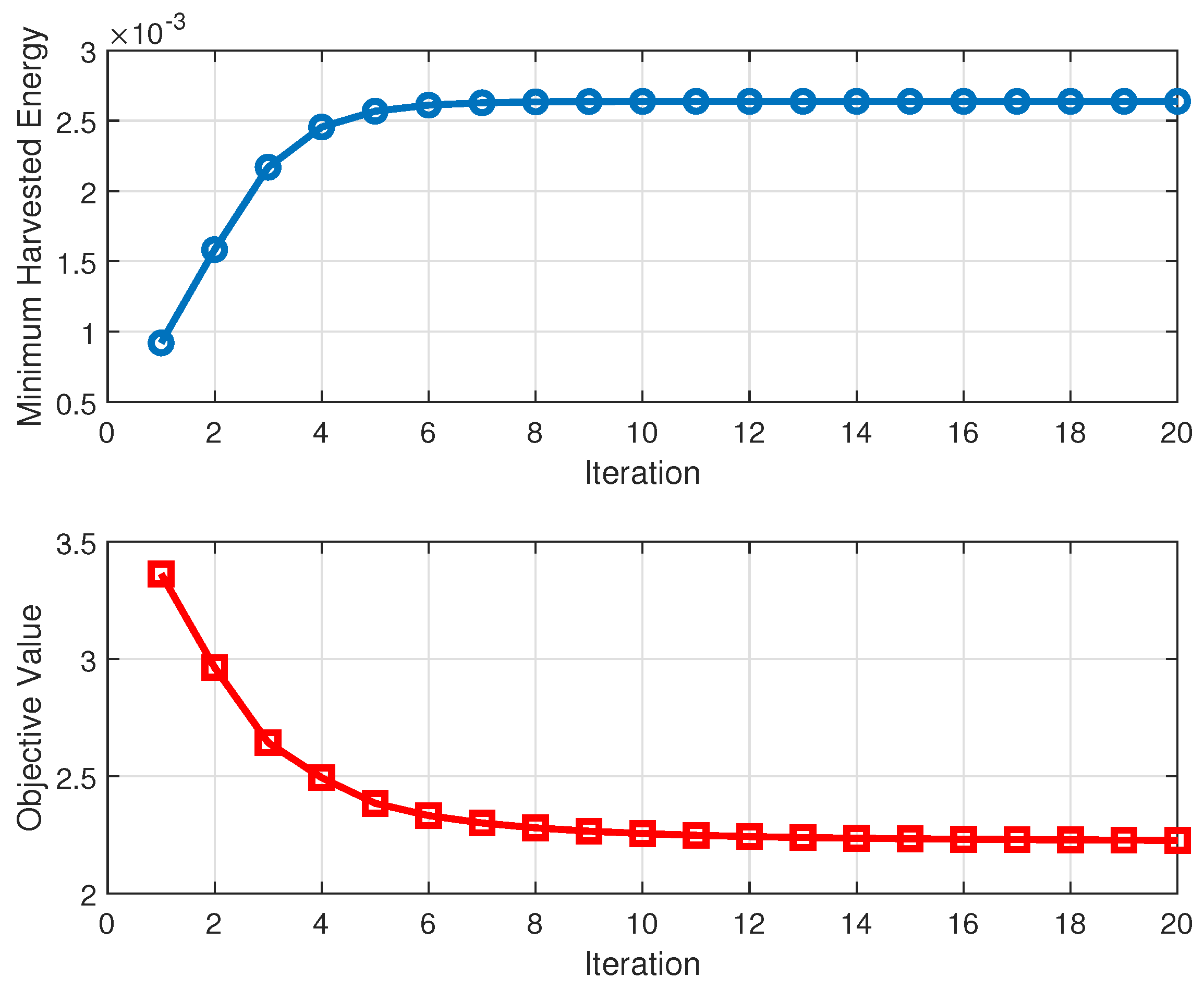
4.1. Max–Min Optimization of SWIPT

For the max–min problem in SWIPT, by introducing the auxiliary variable $e_{\min }$, the original problem ${\mathcal{P}}_{\mathrm{S}}$ can be equivalently rewritten as

$$\begin{array}{cc}\hfill \left({\mathcal{P}}_{\mathrm{S}0}\right)& \underset{\mathbf{v},\mathit{\rho },e_{\min }}{\mathrm{maximize}}{e}_{\min }\hfill \end{array}$$

(40a)

$$\begin{array}{c}\hfill \mathrm{subject}\mathrm{to}\left(38\mathrm{b}\right),\left(38\mathrm{c}\right),\left(38\mathrm{d}\right),\end{array}$$

(40b)

$$\begin{array}{cc}\hfill & \phantom{\mathrm{subject}\mathrm{to}}{E}_{\mathrm{SWIPT}}^k\ge e_{\min },\forall k\in \mathcal{K}.\hfill \end{array}$$

(40c)

Next, we employ the AO method to tackle the previously mentioned non-convex problem by iteratively refining the variables $\mathit{\rho }$, $\mathbf{v}$, and $e_{\min }$ until convergence is achieved. The iterative optimization process for these variables can be categorized into the following two cases.

4.1.1. Given $\mathit{\rho }$, Optimizing ($\mathbf{v},e_{\min }$)

When fixing $\mathit{\rho }$, the optimization problem (${\mathcal{P}}_{\mathrm{S}0}$) simplifies to

$$\begin{array}{cc}\hfill \left({\mathcal{P}}_{\mathrm{S}1}\right)& \underset{\mathbf{v},e_{\min }}{\mathrm{maximize}}{e}_{\min }\hfill \end{array}$$

(41a)

$$\begin{array}{cc}& \mathrm{subject}\mathrm{to}\left(38\mathrm{b}\right),\left(38\mathrm{c}\right),\left(40\mathrm{c}\right).\hfill \end{array}$$

(41b)

Through appropriate mathematical transformations, problem (${\mathcal{P}}_{\mathrm{S}1}$) can be restructured into

$$\begin{array}{cc}\hfill \left({\mathcal{P}}_{\mathrm{S}1.1}\right)& \underset{\mathbf{v},e_{\min }}{\mathrm{maximize}}{e}_{\min }\hfill \end{array}$$

(42a)

$$\begin{array}{c}\hfill \mathrm{subject}\mathrm{to}\left(38\mathrm{c}\right),\end{array}$$

(42b)

$$\begin{array}{cc}\hfill & \phantom{\mathrm{subject}\mathrm{to}}|{\mathbf{h}}_{k,\mathrm{dl}}^H{\mathbf{v}|}^2\ge {\displaystyle \frac{{\gamma }_{\min }({\rho }_k{\sigma }_{\mathrm{dl}}^2+{\sigma }_{\mathrm{pr}}^2)}{{\rho }_k}},\hfill \end{array}$$

(42c)

$$\begin{array}{cc}\hfill & \phantom{\mathrm{subject}\mathrm{to}}|{\mathbf{h}}_{k,\mathrm{dl}}^H{\mathbf{v}|}^2\ge {\displaystyle \frac{e_{\min }-{\phi }_k\left(1-{\rho }_k\right){\sigma }_{\mathrm{dl}}^2}{{\phi }_k\left(1-{\rho }_k\right)}}.\hfill \end{array}$$

(42d)

The primary challenge in addressing the above problem lies in the non-convex constraints (42c) and (42d). To overcome this difficulty, we utilize the SCA method to iteratively update $\mathbf{v}$ by solving a series of approximated convex problems. Specifically, for both non-convex constraints, we construct convex approximations using the first-order Taylor expansion of ${\left|{\mathbf{h}}_{k,\mathrm{dl}}^H\mathbf{v}\right|}^2$. Let ${\mathbf{v}}^{\left(u\right)}$ represent the current beamforming vector at iteration u. Then, we have

$$\begin{array}{c}\hfill {\left|{\mathbf{h}}_{k,\mathrm{dl}}^H\mathbf{v}\right|}^2\ge \underset{\triangleq \mathrm{\Theta }\left(\mathbf{v}\right)}{\underbrace{2\Re \left\{{\mathbf{v}}^{\left(u\right)H}{\mathbf{h}}_{k,\mathrm{dl}}{\mathbf{h}}_{k,\mathrm{dl}}^H(\mathbf{v}-{\mathbf{v}}^{\left(u\right)})\right\}+{\left|{\mathbf{h}}_{k,\mathrm{dl}}^H{\mathbf{v}}^{\left(u\right)}\right|}^2}}.\end{array}$$

(43)

This yields a reconstruction problem with linearized constraints, as

$$\begin{array}{cc}\hfill \left({\mathcal{P}}_{\mathrm{S}1.2}\right)& \underset{\mathbf{v},e_{\min }}{\mathrm{maximize}}{e}_{\min }\hfill \end{array}$$

(44a)

$$\begin{array}{cc}& \mathrm{subject}\mathrm{to}\left(38\mathrm{c}\right),\hfill \end{array}$$

(44b)

$$\begin{array}{cc}\hfill & \phantom{\mathrm{subject}\mathrm{to}}\mathrm{\Theta }\left(\mathbf{v}\right)\ge {\displaystyle \frac{{\gamma }_{\min }({\rho }_k{\sigma }_{\mathrm{dl}}^2+{\sigma }_{\mathrm{pr}}^2)}{{\rho }_k}},\hfill \end{array}$$

(44c)

$$\begin{array}{cc}\hfill & \phantom{\mathrm{subject}\mathrm{to}}\mathrm{\Theta }\left(\mathbf{v}\right)\ge {\displaystyle \frac{e_{\min }-{\phi }_k\left(1-{\rho }_k\right){\sigma }_{\mathrm{dl}}^2}{{\phi }_k\left(1-{\rho }_k\right)}}.\hfill \end{array}$$

(44d)

At this stage, the relaxed problem (${\mathcal{P}}_{\mathrm{S}1.2}$) has been transformed into a convex optimization problem that can be efficiently addressed using the conventional convex optimization solvers, for instance, CVX [39], with polynomial time complexity. By iteratively updating ${\mathbf{v}}^{(u+1)}$ through the solution of the reformulated problem (${\mathcal{P}}_{\mathrm{S}1.2}$), we can identify a local maximum of the original problem (${\mathcal{P}}_{\mathrm{S}1.1}$) once the convergence threshold is reached. Furthermore, the final solution complies with the Karush–Kuhn–Tucker conditions for the problem (${\mathcal{P}}_{\mathrm{S}1.1}$).

4.1.2. Given ($\mathbf{v},e_{\min }$), Optimizing $\mathit{\rho }$

With fixed ($\mathbf{v},e_{\min }$), problem (${\mathcal{P}}_{\mathrm{S}0}$) simplifies to a feasibility-check problem with respect to $\mathit{\rho }$, which does not readily produce an optimal solution. However, we observe that both the SNR constraint and the energy harvesting constraint for each device depend exclusively on its own ${\rho }_k$, without any cross-user dependencies. Therefore, when the beamforming vector $\mathbf{v}$ is fixed, each device can independently optimize its own ${\rho }_k$ to maximize the energy harvested. At this juncture, we can formulate the following optimization problem for device k, as

$$\begin{array}{cc}\hfill \left({\mathcal{P}}_{\mathrm{S}2}\right)& \underset{{\rho }_k}{\mathrm{maximize}}{E}_{\mathrm{SWIPT}}^k\hfill \end{array}$$

(45a)

$$\begin{array}{cc}& \mathrm{subject}\mathrm{to}\left(38\mathrm{b}\right),\left(38\mathrm{d}\right).\hfill \end{array}$$

(45b)

Let ${\alpha }_k\triangleq {\left|{\mathbf{h}}_{k,\mathrm{dl}}^H\mathbf{v}\right|}^2$. The SNR constraint from Equation (38b) can then be expressed as

$$\begin{array}{c}\hfill {\rho }_k\ge {\displaystyle \frac{{\gamma }_{\min }{\sigma }_{\mathrm{pr}}^2}{{\alpha }_k-{\gamma }_{\min }{\sigma }_{\mathrm{dl}}^2}}\triangleq {\rho }_{k,\min }.\end{array}$$

(46)

Maximizing $E_{\mathrm{SWIPT}}^k$ is equivalent to minimizing ${\rho }_k$ while ensuring the SNR constraint is satisfied. Thus, we arrive at the following formulation:

$$\begin{array}{c}\hfill {\rho }_k^{*}=\left\{\begin{array}{cc}0\hfill & \mathrm{if}{\rho }_{k,\min }\le 0,\hfill \\ 1\hfill & \mathrm{if}{\rho }_{k,\min }\ge 1,\hfill \\ {\rho }_{k,\min }\hfill & \mathrm{otherwise}.\hfill \end{array}\right.\end{array}$$

(47)

In summary, the complete algorithm for the alternating optimization for the SWIPT max–min problem is presented in Algorithm 1.

Algorithm 1 Alternating optimization for the SWIPT max–min problem

1: Input: Convergence threshold $ϵ$.   2: Initialize ${\mathit{\rho }}^{\left(0\right)}$, ${\mathbf{v}}^{\left(0\right)}$, iteration index $t\leftarrow 0$   3: while ${\displaystyle \frac{|e_{\min }^{\left(t\right)}-e_{\min }^{(t-1)}|}{|e_{\min }^{(t-1)}|}}>ϵ$ do   4:     Set $u\leftarrow 0$, ${\mathbf{v}}^{\left(u\right)}\leftarrow {\mathbf{v}}^{\left(t\right)}$   5:     while SCA not converged do   6:         Solve convex problem (${\mathcal{P}}_{\mathrm{S}1.2}$) with CVX   7:         Update ${\mathbf{v}}^{(u+1)}\leftarrow {\mathbf{v}}^{*}$, $u\leftarrow u+1$   8:     end while   9:     Set ${\mathbf{v}}^{(t+1)}\leftarrow {\mathbf{v}}^{\left(u\right)}$, $e_{\min }^{(t+1)}\leftarrow e_{\min }^{*}$ 10:     for each device $k\in \mathcal{K}$ do 11:         Calculate ${\rho }_{k,\min }\leftarrow {\displaystyle \frac{{\gamma }_{\min }{\sigma }_{\mathrm{pr}}^2}{{\alpha }_k-{\gamma }_{\min }{\sigma }_{\mathrm{dl}}^2}}$ 12:         Determine $$\begin{array}{c}\hfill {\rho }_k^{(t+1)}=\left\{\begin{array}{cc}0\hfill & \mathrm{if}{\rho }_{k,\min }\le 0,\hfill \\ 1\hfill & \mathrm{if}{\rho }_{k,\min }\ge 1,\hfill \\ {\rho }_{k,\min }\hfill & \mathrm{otherwise}.\hfill \end{array}\right.\end{array}$$ 13:     end for 14:     $t\leftarrow t+1$ 15: end while 16: Output: ${\mathbf{v}}^{*}$, ${\mathit{\rho }}^{*}$

4.2. Joint Learning–Communication Optimization

After solving the SWIPT max–min optimization problem, we denote the optimal total energy harvested by device k as $E_{\mathrm{SWIPT}}^{k*}$. The next step is to minimize the convergence error $\mathcal{G}$ while adhering to the available energy constraint of device k, which is given by $E_{\mathrm{com}}^k+E_{\mathrm{comp}}^k\le E_{\mathrm{local}}^k+E_{\mathrm{SWIPT}}^{k*}$. This is achieved by jointly optimizing the transmit equalization coefficient $\mathbf{p}$, the receiver beamforming $\mathbf{f}$, and the local training accuracy $\mathit{\theta }$. Given the coupling between the computational and communication optimization variables at this stage, this paper proposes an alternating optimization framework, which is divided into two main phases: a wireless transmission design and local training intensity optimization.

4.2.1. Wireless Transmission Design

With a fixed local training accuracy, $\mathit{\theta }$, our goal is to minimize the AirComp MSE $\widetilde{\mathbb{MSE}}(x\left[d\right],\widehat{x}\left[d\right])$ by adjusting the wireless transmission strategy, which includes the transmit equalization coefficient $\mathbf{p}$ and the receive beamforming $\mathbf{f}$. This problem is formulated as

$$\begin{array}{cc}\hfill \left({\mathcal{P}}_{T0}\right)& \underset{\mathbf{p},\mathbf{f}}{\mathrm{minimize}}\widetilde{\mathbb{MSE}}(x\left[d\right],\widehat{x}\left[d\right])\hfill \end{array}$$

(48a)

$$\begin{array}{cc}& \mathrm{subject}\mathrm{to}\left(39\mathrm{b}\right),\left(39\mathrm{c}\right).\hfill \end{array}$$

(48b)

The problem (${\mathcal{P}}_{T0}$) still involves two interdependent optimization variables, including the transmit equalization coefficient $\mathbf{p}$ and the receive beamforming $\mathbf{f}$. Therefore, we will continue to adopt an alternating iteration approach, which allows us to progressively optimize each variable in turn.

Given transmit equalization coefficient $\mathbf{p}$, the optimization problem regarding the receive beamforming vector $\mathbf{f}$ can be formulated as

$$\begin{array}{cc}\hfill \left({\mathcal{P}}_{T1}\right)& \underset{\mathbf{f}}{\mathrm{minimize}}\mathbb{MSE}(x\left[d\right],\widehat{x}\left[d\right])\hfill \end{array}$$

(49a)

$$\begin{array}{cc}& \mathrm{subject}\mathrm{to}\left(39\mathrm{c}\right).\hfill \end{array}$$

(49b)

To efficiently solve the above optimization problem, we define the following auxiliary variable as $\mathit{\varphi }={\displaystyle \sum _{k\in \mathcal{K}}}{\mathbf{h}}_{k,\mathrm{d}}{p}_k$. Through appropriate mathematical transformations, the problem $\left({\mathcal{P}}_{T1}\right)$ can be reformulated as

$$\left({\mathcal{P}}_{T1.1}\right)\underset{\mathbf{f}}{\mathrm{minimize}}{O}_{\mathbf{f}}\mathrm{subject}\mathrm{to}{C}_{\mathbf{f}}\le 0,$$

(50)

with

$$\begin{array}{cc}\hfill O_{\mathbf{f}}& ={\mathbf{f}}^H\mathbf{\Omega }\mathbf{f}-2\Re \left\{{\mathbf{f}}^H\mathit{\varphi }\right\},\hfill \end{array}$$

(51)

$$\begin{array}{cc}\hfill C_{\mathbf{f}}& =\left(r_a-1\right){\mathbf{f}}^H\mathbf{\Omega }\mathbf{f}-2r_a\Re \left\{{\mathbf{f}}^H\mathit{\varphi }\right\}+r_{a}K,\hfill \end{array}$$

(52)

where

$$\mathbf{\Omega }\triangleq \sum _{k\in \mathcal{K}}{\left|p_k\right|}^2{\mathbf{h}}_{k,d}{\mathbf{h}}_{k,d}^H+{\sigma }^2\mathbf{I}.$$

(53)

Here, $r_a={\max }_k{2}^{{\displaystyle \frac{{\left|p_k\right|}^{2}S}{B_{\mathrm{ul}}\left(E_{\mathrm{local}}^k+E_{\mathrm{SWIPT}}^k-E_{\mathrm{comp}}^k\right)}}}$. At this point, the objective function of problem (${\mathcal{P}}_{T1.1}$) has taken the form of a standard quadratic function, and its constraints constitute a convex set, which can be efficiently solved with CVX.

With the optimal receiver beamforming $\mathbf{f}$, we need to solve the following simplified problem:

$$\begin{array}{cc}\hfill \left({\mathcal{P}}_{T1.3}\right)& \underset{\mathbf{p}}{\mathrm{minimize}}\mathbb{MSE}(r\left[d\right],\widehat{r}\left[d\right])\hfill \end{array}$$

(54a)

$$\begin{array}{cc}& \mathrm{subject}\mathrm{to}\left(39\mathrm{b}\right),\left(39\mathrm{c}\right).\hfill \end{array}$$

(54b)

Due to the presence of the non-convex constraint (39c), the problem (${\mathcal{P}}_{T1.3}$) poses significant challenges. To effectively mitigate the complexity of the solution process, we next introduce an auxiliary variable $\mu \le R_{\mathrm{ul}}$. Consequently, the problem (${\mathcal{P}}_{T1.3}$) can be equivalently reformulated in the following manner:

$$\begin{array}{cc}\hfill \left({\mathcal{P}}_{T1.4}\right)& \underset{\mathbf{p},\mu }{\mathrm{minimize}}\mathbb{MSE}(x\left[d\right],\widehat{x}\left[d\right])\hfill \end{array}$$

(55a)

$$\begin{array}{cc}& \mathrm{subject}\mathrm{to}\left(39\mathrm{b}\right),\mu \le R_{\mathrm{ul}},\hfill \end{array}$$

(55b)

$$\begin{array}{c}\hfill \phantom{\mathrm{subject}\mathrm{to}}{\left|p_k\right|}^{2}S-E_{\mathrm{maxt}}^k{B}_{\mathrm{ul}}\mu \le 0,\end{array}$$

(55c)

where we define $E_{\mathrm{maxt}}^k=E_{\mathrm{local}}^k+E_{\mathrm{SWIPT}}^k-E_{\mathrm{comp}}^k$.

Next, we gradually adjust the values of $\mu$ and $\mathbf{p}$ through alternating iterations to approximate the optimal solution of problem (${\mathcal{P}}_{T1.4}$). Given a specific value of $\mu$, we can apply appropriate mathematical transformations to simplify problem (${\mathcal{P}}_{T1.4}$) to the following form:

$$\begin{array}{cc}\hfill \left({\mathcal{P}}_{T1.5}\right)& \underset{\mathbf{p}}{\mathrm{minimize}}\mathbb{MSE}(x\left[d\right],\widehat{x}\left[d\right])\hfill \end{array}$$

(56a)

$$\begin{array}{cc}& \mathrm{subject}\mathrm{to}\left(39\mathrm{b}\right),\left(55\mathrm{c}\right),\hfill \end{array}$$

(56b)

$$\begin{array}{c}\hfill \phantom{\mathrm{subject}\mathrm{to}}{C}_{\mathbf{p}}\le 0,\end{array}$$

(56c)

where

$$\begin{array}{cc}\hfill & C_{\mathbf{p}}=\sum _{k\in \mathcal{K}}\left[\left(r_b-1\right){\left|{\mathbf{f}}^H{\mathbf{h}}_{k,d}{p}_k\right|}^2-2r_b\mathcal{R}e\left\{{\mathbf{f}}^H{\mathbf{h}}_{k,d}{p}_k\right\}+r_b\right]+\left(r_b-1\right){\sigma }^2{∥\mathbf{f}∥}^2,\hfill \end{array}$$

(57)

with $r_b=2^{\mu }$. Now, problem (${\mathcal{P}}_{T1.4}$) has been transformed into a standard convex optimization problem (${\mathcal{P}}_{T1.5}$). This new formulation can be efficiently solved using CVX.

After determining $\mathbf{p}$, the auxiliary variable $\mu$ can be straightforwardly updated to $\mu =R_{\mathrm{ul}}$. We now present the following lemma to demonstrate that, by alternately optimizing $\mathbf{p}$ and $\mu$, one can gradually approach the optimal solution of problem (${\mathcal{P}}_{T1.4}$).

Lemma 2.

By alternately updating $\mathit{p}$ and μ, a convergent solution can eventually be obtained.

Proof. 

Assuming that, in the $(t-1)$-th alternating iteration, the solution set for $\mathbf{p}$ and $\mu$ is denoted as $\{{\mathbf{p}}^{t-1},{\mu }^{t-1}\}$, with the corresponding objective function value being ${\widetilde{\mathbb{MSE}}}^{t-1}$, where we define ${\widetilde{\mathbb{MSE}}}^{t-1}={\mathbb{MSE}}^{t-1}(x\left[d\right],\widehat{x}\left[d\right])$. According to the update rule, the auxiliary variable satisfies ${\mu }^{t-1}=R_{\mathrm{ul}}\left({\mathbf{p}}^{t-1}\right)$. In the subsequent t-th iteration, if problem $\left({\mathcal{P}}_{T1.4}\right)$ has a feasible solution ${\mathbf{p}}^t$ at ${\mu }^{t-1}$, then the solution ${\mathbf{p}}^t$ satisfies ${\mu }^{t-1}=R_{\mathrm{ul}}\left({\mathbf{p}}^t\right)$ or ${\mu }^{t-1}<R_{\mathrm{ul}}\left({\mathbf{p}}^t\right)$. If ${\mu }^{t-1}=R_{\mathrm{ul}}\left({\mathbf{p}}^t\right)$, then the current solution ${\mathbf{p}}^t$ is consistent with the previous solution ${\mathbf{p}}^{t-1}$, indicating that the system has found an extremum point. Conversely, if ${\mu }^{t-1}<R_{\mathrm{ul}}\left({\mathbf{p}}^t\right)$, this suggests that the current solution ${\mathbf{p}}^t$ constitutes an improvement over the previous solution ${\mathbf{p}}^{t-1}$, leading to a further reduction in the objective function value, i.e., ${\widetilde{\mathbb{MSE}}}^t<{\widetilde{\mathbb{MSE}}}^{t-1}$. Thus, by continuously updating $\mathbf{p}$ and $\mu$, the system ensures that $\widetilde{\mathbb{MSE}}$ decreases with each iteration. Furthermore, since the objective function $\widetilde{\mathbb{MSE}}$ is non-negative and has a minimum value that serves as a lower bound, the objective function value will not decrease indefinitely. Based on this, it can be deduced that, with the alternating iterative updates of $\mathbf{p}$ and $\mu$, the system will ultimately converge to a global optimal solution or a local optimal solution. □

4.2.2. Local Training Intensity Determination

Given the transmit equalization factor $\mathbf{p}$ and the receiver beamforming $\mathbf{f}$, the problem of optimizing the local accuracy vector $\mathit{\theta }$ can be simplified to

$$\begin{array}{cc}\hfill \left({\mathcal{P}}_2\right)& \underset{\mathit{\theta }}{\mathrm{maximize}}\mathrm{\Phi }\hfill \end{array}$$

(58a)

$$\begin{array}{cc}& \mathrm{subject}\mathrm{to}\left(39\mathrm{c}\right),\left(39\mathrm{d}\right),\left(39\mathrm{e}\right).\hfill \end{array}$$

(58b)

Due to the involvement of multiple summation terms, squared terms, and complex parameter dependencies in the objective function $\mathrm{\Phi }$, directly optimizing this function poses significant challenges. Additionally, the nonlinear nature of the constraint $0<\mathrm{\Phi }<1$ further complicates the problem, making it difficult to simultaneously satisfy both the objective function and the constraint. To address these issues, we propose a simplified strategy based on parameter tuning. By appropriately setting the value ranges of key hyperparameters, the constraints concerning $\mathrm{\Phi }$ can be naturally satisfied during the optimization process, thus avoiding the complexities associated with directly solving the original problem. Next, we will focus on ensuring that $\mathrm{\Phi }$ remains within the interval $0<\mathrm{\Phi }<1$ by suitably adjusting the value range for the hyperparameter $\eta$, as illustrated in the following lemma.

Lemma 3.

With Assumption 1, if we set

$$\begin{array}{c}\hfill \eta <{\displaystyle \frac{\frac{1}{K}{\displaystyle \sum _{k=1}^K}\left[2{({\theta }_k-1)}^2-{\rho }^2{\theta }_k(1+{\theta }_k)\right]}{\frac{1}{K}{\displaystyle \sum _{k=1}^K}\left[3{\rho }^2{\theta }_k(1+{\theta }_k)+3{\rho }^2(1+{\theta }_k)\right]}},\end{array}$$

(59)

the convergence condition $0<\mathrm{\Phi }<1$ is always satisfied.

Proof of Lemma 3.

See Appendix B. □

Next, from constraint (39c) and constraint (39d), we can derive

$${\theta }_k\ge {\displaystyle \frac{C}{e^{\frac{E_{\mathrm{local}}^k+E_{\mathrm{SWIPT}}^k-E_{com}^k}{\frac{{\alpha }_k}{\gamma }{c}_k{D}_k{f}_k^2}}}},{\theta }_k\ge {\displaystyle \frac{C}{e^{\frac{T\gamma f_k}{2c_k{D}_k}}}}.$$

(60)

It should be noted that the local accuracy ${\theta }_k$ for each device is completely decoupled, meaning that each device can independently choose the optimal ${\theta }_k$ based on its own computational resources and energy constraints, without relying on the choices of other devices. By analyzing the form of $\mathrm{\Phi }$, it can be observed that, within the range $0<{\theta }_k<1,\forall k\in \mathcal{K}$, $\mathrm{\Phi }$ monotonically increases as ${\theta }_k$ decreases. In other words, the smaller the value of ${\theta }_k$, the larger the value of $\mathrm{\Phi }$, which contributes to the improvement of system performance. Therefore, when selecting ${\theta }_k$, each device will prioritize choosing the minimum value that satisfies the lower bound of the constraint, i.e.,

$${\theta }_k=min\left\{1,max\left\{{\displaystyle \frac{C}{e^{\frac{E_{\mathrm{local}}^k+E_{\mathrm{SWIPT}}^k-E_{com}^k}{\frac{{\alpha }_k}{\gamma }{c}_k{D}_k{f}_k^2}}}},{\displaystyle \frac{C}{e^{\frac{T\gamma f_k}{2c_k{D}_k}}}}\right\}\right\},\forall k\in \mathcal{K}.$$

(61)

Accordingly, we can summarize the basic process of the joint learning–communication optimization, as outlined in Algorithm 2.

Algorithm 2 Joint Learning–Communication Optimization

1: Input: Convergence threshold $ϵ$   2: Initialize ${\mathbf{p}}^{\left(0\right)}$, ${\mathit{\theta }}^{\left(0\right)}$, iteration index $u\leftarrow 0$   3: while ${\displaystyle \frac{|{\mathcal{G}}^{\left(u\right)}-{\mathcal{G}}^{(u-1)}|}{|{\mathcal{G}}^{(u-1)}|}}>ϵ$ do   4:     Solve convex problem (${\mathcal{P}}_{T1.1}$) with CVX   5:     Update ${\mathbf{f}}^{(u+1)}\leftarrow {\mathbf{f}}^{*}$   6:     Set ${\mu }^{\left(0\right)}\leftarrow R_{\mathrm{ul}}$, $t\leftarrow 0$   7:     while ${\displaystyle \frac{|{\widetilde{\mathbb{MSE}}}^t-{\widetilde{\mathbb{MSE}}}^{t-1}|}{|{\widetilde{\mathbb{MSE}}}^{t-1}|}}>ϵ$ do   8:         Solve convex problem (${\mathcal{P}}_{T1.5}$) with CVX   9:         Update ${\mathbf{p}}^{(t+1)}\leftarrow {\mathbf{p}}^{*}$, ${\mu }^{(t+1)}\leftarrow R_{\mathrm{ul}}$ 10:         $t\leftarrow t+1$ 11:     end while 12:     Set ${\mathbf{p}}^{(u+1)}\leftarrow {\mathbf{p}}^{\left(t\right)}$ 13:     for each device $k\in \mathcal{K}$ do 14:         Determine optimal local accuracy 15:         ${\theta }_k^{(u+1)}=min\left\{1,max\left\{{\displaystyle \frac{C}{e^{\frac{E_{\mathrm{local}}^k+E_{\mathrm{SWIPT}}^k-E_{com}^k}{\frac{{\alpha }_k}{\gamma }{c}_k{D}_k{f}_k^2}}}},{\displaystyle \frac{C}{e^{\frac{T\gamma f_k}{2c_k{D}_k}}}}\right\}\right\}$, 16:     end for 17:     $u\leftarrow u+1$ 18: end while 19: Output:${\mathbf{p}}^{*}$, ${\mathbf{f}}^{*}$, ${\mathit{\theta }}^{*}$

4.3. Computational Complexity

Based on the previous analysis, both problems (${\mathcal{P}}_{\mathrm{S}}$) and (${\mathcal{P}}_{\mathrm{T}}$) can be progressively optimized using an AO algorithm, with their optimization processes summarized in Algorithm 1 and Algorithm 2, respectively.

For Algorithm 1, its computational complexity is primarily determined by the stepwise solution of the subproblem (${\mathcal{P}}_{S1.2}$). The complexity of solving this convex problem has a complexity of $\mathcal{O}\left(I_v{J}^{3.5}\right)$, where $I_v$ denotes the number of SCA iterations. After $t^{\max }$ alternating iterations, the overall worst-case complexity of Algorithm 1 can be expressed as $\mathcal{O}\left(t^{\max }\left(I_v{J}^{3.5}\right)\right)$. Here, we neglect the complexity of the assignment operation in Equation (47).

For Algorithm 2, its computational complexity mainly arises from the stepwise solution of the subproblems (${\mathcal{P}}_{T1.1}$) and (${\mathcal{P}}_{T1.5}$). According to [34], the worst-case computational complexity for solving the subproblem (${\mathcal{P}}_{T1.1}$) using the interior point method is $\mathcal{O}\left(J^{3.5}\right)$. Similarly, the worst-case complexity for solving the subproblem (${\mathcal{P}}_{T1.5}$) is $\mathcal{O}\left(I_p{K}^{3.5}\right)$, where $I_p$ is the number of alternating iterations required when solving for $\mathbf{p}$. In contrast, the computational complexity associated with the assignment operations in solving the subproblem (${\mathcal{P}}_2$) is relatively low and can be ignored. In summary, assuming Algorithm 2 converges within $u^{\max }$ iterations, the final overall worst-case complexity can be expressed as $\mathcal{O}\left(u^{\max }(J^{3.5}+I_p{K}^{3.5})\right)$.

5. Numerical Results

In this section, we exhibit numerical experiments to validate the effectiveness of our proposed system design.

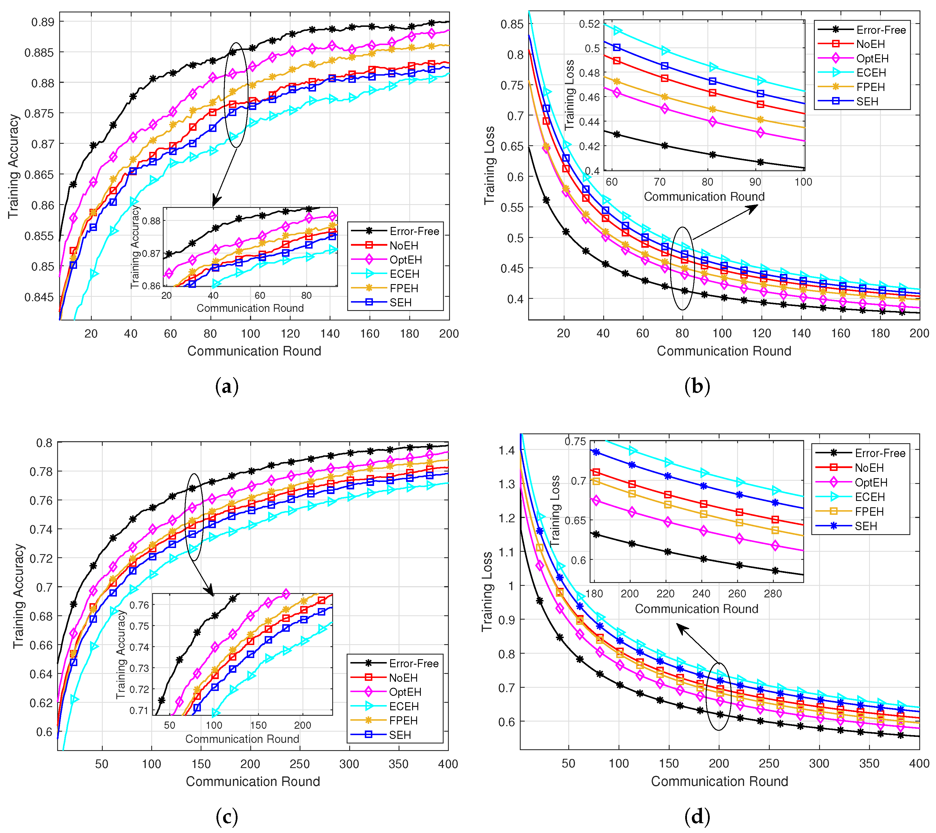
5.1. Simulation Setup

We create a three-dimensional simulation environment where the BS is positioned at coordinates (0, 0, 0), and $K=6$ edge devices are uniformly and randomly positioned along half-circles with a radius of $10 \mathrm{m}$ around the BS. The channels involved in the system, specifically ${\mathbf{h}}_{k,\mathrm{dl}}$ and ${\mathbf{h}}_{k,\mathrm{d}}$, are modeled as Rician fading channels [40]. The path loss, which depends on distance, is expressed as $L\left(d\right)={\zeta }_0{\left(d/d_0\right)}^{-\alpha }$, where ${\zeta }_0$ denotes the reference path loss at a distance $d_0=1$ m, d represents the link distance, and $\alpha$ is the path loss exponent. Unless stated otherwise, the following parameter values are used: $P_0=20$ dBm, $P_{\max }=50$ dBm, ${\sigma }_{\mathrm{dl}}^2={\sigma }_{\mathrm{pr}}^2=-80$ dBm, ${\zeta }_0=-30$ dB, $\alpha =3.5$, $J=6$, $B_{\mathrm{ul}}=6$ mHz, $T_{max}=0.03$ s, $E_{\mathrm{local}}^k=0.04$ J, ${\phi }_k=0.8$, 1 GHz $\le f_k\le$ 3 GHz, $\forall k$, and $ϵ=1e-5$.

Our approach is evaluated through an image classification task utilizing the well-known MNIST dataset [41] as well as the Fashion-MNIST dataset [42]. For both datasets, we employ a multinomial logistic regression model with a dimensionality of $D=7850$, paired with a cross-entropy loss function [5]. Additionally, the local training data for each edge device is sampled independently and identically from the training set, with each device receiving a total of 600 training samples. For both datasets, we utilized the standard test set, which consists of 10,000 images. The experiment implementation is conducted using PyTorch 1.12.1 on a Legion Y9000P IAH7H laptop (manufactured by Lenovo, Beijing, China), which is equipped with an NVIDIA GeForce RTX 3060 Laptop GPU (manufactured by NVIDIA, Santa Clara, CA, USA) with 6 GB of memory. All experimental curves presented in the paper represent the average results of five MonteCarlo simulations.

To comprehensively evaluate the effectiveness of the proposed algorithm (OptEH), we compare it with the following baseline methods:

• NoEH [6]: In this approach, edge devices have only limited inherent energy and cannot replenish their energy during the FEEL processes.
• ECEH [5]: All devices adopt the same energy harvesting scheme and wireless communication strategy as OptEH, but they execute the same local training intensity, which is determined by the slowest device.
• FPEH [43]: This scheme implements a heuristic approach to SWIPT by employing a fixed power-splitting ratio. In this model, devices operate with a predetermined ratio for splitting power between energy harvesting and information decoding (we set ${\rho }_k=0.1,\forall k$).
• SEH [44]: Devices are selected based on their channel gain to mitigate the “straggler” problem. Only those devices that achieve channel gains above a specified threshold are allowed to participate in the training process, while others are excluded from engagement in training.

Additionally, we compare a scenario where the local training intensity is the same as that of OptEH in an ideal environment without channel noise (referred to as Error-Free) to assess the impact of communication noise and interference on the FEEL learning performance.

5.2. Convergence Behaviour of the Proposed Algorithms

We start by validating the convergence performance of the proposed Algorithms 1 and 2. Figure 2 illustrates the convergence curves of both algorithms across different numbers of alternating iterations. The simulation results indicate that, as expected, our proposed algorithms converge to a stable value within a relatively small number of iterations (approximately seven iterations). This behavior aligns with the theoretical convergence analysis, thereby confirming the effectiveness of the proposed algorithms.

5.3. Performance Comparison on Learning Convergence

As illustrated in Figure 3, we present the testing accuracy and training loss of the proposed algorithm in comparison to baseline algorithms across different datasets. The results clearly indicate that the proposed algorithm outperforms the baseline methods regarding convergence performance. Compared to NoEH, our method demonstrates a significant performance gain. This improvement is primarily attributed to the fact that, with energy harvesting, our system can support more frequent local updates while maintaining a higher power level during the communication process. In contrast to ECEH, our approach allows devices to conduct local training to the fullest extent based on their individual computational capacity and available energy. This flexibility facilitates a more effective utilization of each device’s computational resources, thereby enhancing the overall efficiency of the system. The results from comparing our approach with FPEH highlight the significance of appropriately selecting the device’s power splitting in SWIPT for the FEEL system. This dynamic adjustment allows devices to optimize the trade-off between EH and ID based on their current energy status and channel conditions. When compared to SEH, our approach demonstrates superior performance. This discrepancy may stem from the fact that, while SEH may exclude devices with lower channel gains to enhance the overall communication quality of the system, such exclusion also reduces the diversity of the training data. When the performance gains from improved communication quality do not sufficiently compensate for the performance losses associated with decreased data diversity, it can lead to suboptimal learning outcomes. Moreover, when compared to the ideal Error-Free scenario, the proposed algorithm reveals a small yet significant performance gap. This discrepancy primarily arises from the interference caused by wireless channel conditions affecting model updates during FEEL training, which is consistent with the theoretical analysis outlined in Theorem 1.

5.4. Performance Versus the Number of BS Antennas

As shown in Figure 4a,b, we further analyze the impact of varying numbers of BS antennas on the training performance of the proposed method. The results indicate that, as the number of receiving antennas at the BS increases, the learning performance of all schemes improves significantly. This enhancement is primarily attributed to the additional multiplexing gain provided via the BS antennas, which effectively strengthens the signal reception capacity and reduces transmission distortion during the model update process. Notably, compared to other baseline methods, the proposed optimization framework demonstrates a more pronounced performance advantage as the number of BS antennas increases.

5.5. Performance Versus the Maximum Inherent Energy Budget

Figure 4c,d illustrate the impact of the maximum inherent energy budget $E_{\mathrm{local}}^k$ for all devices $k\in \mathcal{K}$ on the learning performance, measured using the test accuracy on both datasets. For simplification, we assume that all devices have the same $E_{\mathrm{local}}^k$ and denote it as $E_{\mathrm{local}}$. The results show that, as $E_{\mathrm{local}}$ increases, the performance of all methods improves significantly. This enhancement is primarily due to the higher energy budget, which relaxes the energy constraints on devices during wireless communication. This relaxation allows for higher transmission power and increased local training intensity, thereby boosting overall system performance. However, after a certain threshold is reached, further increases in $E_{\mathrm{local}}$ lead to diminishing returns. This phenomenon is attributed to the physical limitations of device communication capacity, indicating that, beyond a certain energy budget, the MSE cannot be further reduced. In other words, increasing the energy budget does not always yield linear gains in performance.

6. Conclusions

In this paper, we proposed a novel asymmetry-tolerance training framework for FEEL that was enabled via SWIPT. This framework leveraged SWIPT to provide sustainable energy support for devices while accommodating varying local training intensities. Then, we rigorously derived a new explicit upper bound that captured the combined effects of local training accuracy and the MSE of the wireless aggregation on the convergence performance of FEEL to highlight the importance of the joint design of learning and communication. Furthermore, we formulated two key optimization problems: the first aimed to maximize the energy harvesting capability among all devices, while the second addressed the joint learning and communication optimization problem under the optimal energy harvesting strategy. Finally, comprehensive experiments demonstrated that our proposed framework achieved significant performance improvements compared to the existing baselines.

For future research, the following areas are worthy of further exploration: (1) introducing reconfigurable intelligent surfaces to enhance the wireless communication environment and thereby potentially improving the efficiency of energy harvesting and contributing to better overall performance in heterogeneous training frameworks, (2) developing intelligent device selection algorithms that utilize machine learning to predict which devices are most likely to meet energy requirements under varying channel conditions and thereby ensuring optimal participation from devices, (3) on this basis, exploring the integration of multi-source energy harvesting techniques and allowing devices to leverage various energy sources simultaneously, which could lead to more sustainable and resilient operation in diverse environments.

References

1. Lyu, X.; Ren, C.; Ni, W.; Tian, H.; Liu, R.P.; Dutkiewicz, E. Optimal Online Data Partitioning for Geo-Distributed Machine Learning in Edge of Wireless Networks. IEEE J. Sel. Areas Commun. 2019, 37, 2393–2406. [Google Scholar] [CrossRef]
2. Li, T.; Sahu, A.K.; Talwalkar, A.; Smith, V. Federated Learning: Challenges, Methods, and Future Directions. IEEE Signal Process. Mag. 2020, 37, 50–60. [Google Scholar] [CrossRef]
3. Zhang, T.; Mao, S. Energy-Efficient Federated Learning With Intelligent Reflecting Surface. IEEE Trans. Green Commun. Netw. 2022, 6, 845–858. [Google Scholar] [CrossRef]
4. McMahan, B.; Moore, E.; Ramage, D.; Hampson, S.; Arcas, B.A.y. Communication-Efficient Learning of Deep Networks from Decentralized Data. In Proceedings of the 20th International Conference on Artificial Intelligence and Statistics, Lauderdale, FL, USA, 20–22 April 2017; Singh, A., Zhu, J., Eds.; PMLR: Mc Kees Rocks, PA, USA, 2017; Volume 54, pp. 1273–1282. [Google Scholar]
5. Dinh, C.T.; Tran, N.H.; Nguyen, M.N.H.; Hong, C.S.; Bao, W.; Zomaya, A.Y.; Gramoli, V. Federated Learning Over Wireless Networks: Convergence Analysis and Resource Allocation. IEEE/ACM Trans. Netw. 2021, 29, 398–409. [Google Scholar] [CrossRef]
6. Li, H.; Wang, R.; Jiang, M.; Liu, J. STAR-RIS Empowered Heterogeneous Federated Edge Learning With Flexible Aggregation. IEEE Internet Things J. 2025, 12, 28374–28389. [Google Scholar] [CrossRef]
7. Zhou, Y.; Pang, X.; Wang, Z.; Hu, J.; Sun, P.; Ren, K. Towards Efficient Asynchronous Federated Learning in Heterogeneous Edge Environments. In Proceedings of the IEEE INFOCOM 2024—IEEE Conference on Computer Communications, Vancouver, BC, Canada, 20–23 May 2024; pp. 2448–2457. [Google Scholar]
8. Lu, Y.; Huang, X.; Dai, Y.; Maharjan, S.; Zhang, Y. Differentially Private Asynchronous Federated Learning for Mobile Edge Computing in Urban Informatics. IEEE Trans. Ind. Informatics 2020, 16, 2134–2143. [Google Scholar] [CrossRef]
9. Kou, Z.; Ji, Y.; Yang, D.; Zhang, S.; Zhong, X. Semi-Asynchronous Over-the-Air Federated Learning Over Heterogeneous Edge Devices. IEEE Trans. Veh. Technol. 2025, 74, 110–125. [Google Scholar] [CrossRef]
10. Wang, Z.; Zhang, Z.; Tian, Y.; Yang, Q.; Shan, H.; Wang, W.; Quek, T.Q.S. Asynchronous Federated Learning Over Wireless Communication Networks. IEEE Trans. Wirel. Commun. 2022, 21, 6961–6978. [Google Scholar] [CrossRef]
11. Chen, Z.; Yi, W.; Shin, H.; Nallanathan, A. Adaptive Semi-Asynchronous Federated Learning over Wireless Networks. IEEE Trans. Commun. 2024, 73, 394–409. [Google Scholar] [CrossRef]
12. Xu, Y.; Liao, Y.; Xu, H.; Ma, Z.; Wang, L.; Liu, J. Adaptive Control of Local Updating and Model Compression for Efficient Federated Learning. IEEE Trans. Mob. Comput. 2023, 22, 5675–5689. [Google Scholar] [CrossRef]
13. Ma, Z.; Xu, Y.; Xu, H.; Meng, Z.; Huang, L.; Xue, Y. Adaptive Batch Size for Federated Learning in Resource-Constrained Edge Computing. IEEE Trans. Mob. Comput. 2023, 22, 37–53. [Google Scholar] [CrossRef]
14. Wang, L.; Xu, Y.; Xu, H.; Jiang, Z.; Chen, M.; Zhang, W.; Qian, C. BOSE: Block-Wise Federated Learning in Heterogeneous Edge Computing. IEEE/ACM Trans. Netw. 2024, 32, 1362–1377. [Google Scholar] [CrossRef]
15. Liao, Y.; Xu, Y.; Xu, H.; Wang, L.; Qian, C. Adaptive Configuration for Heterogeneous Participants in Decentralized Federated Learning. In Proceedings of the IEEE INFOCOM 2023—IEEE Conference on Computer Communications, New York, NY, USA, 17–20 May 2023; pp. 1–10. [Google Scholar]
16. Zeng, M.; Wang, X.; Pan, W.; Zhou, P. Heterogeneous Training Intensity for Federated Learning: A Deep Reinforcement Learning Approach. IEEE Trans. Netw. Sci. Eng. 2023, 10, 990–1002. [Google Scholar] [CrossRef]
17. Li, H.; Wang, R.; Zhang, W.; Wu, J. One Bit Aggregation for Federated Edge Learning With Reconfigurable Intelligent Surface: Analysis and Optimization. IEEE Trans. Wirel. Commun. 2023, 22, 872–888. [Google Scholar] [CrossRef]
18. Chen, M.; Yang, Z.; Saad, W.; Yin, C.; Poor, H.V.; Cui, S. A Joint Learning and Communications Framework for Federated Learning Over Wireless Networks. IEEE Trans. Wirel. Commun. 2021, 20, 269–283. [Google Scholar] [CrossRef]
19. Wen, D.; Bennis, M.; Huang, K. Joint Parameter-and-Bandwidth Allocation for Improving the Efficiency of Partitioned Edge Learning. IEEE Trans. Wirel. Commun. 2020, 19, 8272–8286. [Google Scholar] [CrossRef]
20. Li, H.; Wang, R.; Wu, J.; Zhang, W.; Soto, I. Reconfigurable Intelligent Surface Empowered Federated Edge Learning With Statistical CSI. IEEE Trans. Wirel. Commun. 2024, 23, 6595–6608. [Google Scholar] [CrossRef]
21. Yang, K.; Jiang, T.; Shi, Y.; Ding, Z. Federated Learning via Over-the-Air Computation. IEEE Trans. Wirel. Commun. 2020, 19, 2022–2035. [Google Scholar] [CrossRef]
22. Zhu, G.; Du, Y.; Gündüz, D.; Huang, K. One-Bit Over-the-Air Aggregation for Communication-Efficient Federated Edge Learning: Design and Convergence Analysis. IEEE Trans. Wirel. Commun. 2021, 20, 2120–2135. [Google Scholar] [CrossRef]
23. Liang, Y.; Chen, Q.; Zhu, G.; Jiang, H.; Eldar, Y.C.; Cui, S. Communication-and-Energy Efficient Over-the-Air Federated Learning. IEEE Trans. Wirel. Commun. 2025, 24, 767–782. [Google Scholar] [CrossRef]
24. Zhang, Y.; You, C. SWIPT in Mixed Near- and Far-Field Channels: Joint Beam Scheduling and Power Allocation. IEEE J. Sel. Areas Commun. 2024, 42, 1583–1597. [Google Scholar] [CrossRef]
25. Faramarzi, S.; Zarini, H.; Javadi, S.; Robat Mili, M.; Zhang, R.; Karagiannidis, G.K.; Al-Dhahir, N. Energy Efficient Design of Active STAR-RIS-Aided SWIPT Systems. IEEE Trans. Wirel. Commun. 2025, 24, 3209–3224. [Google Scholar] [CrossRef]
26. He, Y.; Huang, F.; Wang, D.; Zhang, R. Outage Probability Analysis of MISO-NOMA Downlink Communications in UAV-Assisted Agri-IoT With SWIPT and TAS Enhancement. IEEE Trans. Netw. Sci. Eng. 2025, 12, 2151–2164. [Google Scholar] [CrossRef]
27. Do, T.N.; da Costa, D.B.; Duong, T.Q.; An, B. Improving the Performance of Cell-Edge Users in MISO-NOMA Systems Using TAS and SWIPT-Based Cooperative Transmissions. IEEE Trans. Green Commun. Netw. 2018, 2, 49–62. [Google Scholar] [CrossRef]
28. Zheng, G.; Fang, Y.; Wen, M.; Ding, Z. Novel Over-the-Air Federated Learning via Reconfigurable Intelligent Surface and SWIPT. IEEE Internet Things J. 2024, 11, 34140–34155. [Google Scholar] [CrossRef]
29. Liu, H.; Yuan, X.; Zhang, Y.J.A. Reconfigurable Intelligent Surface Enabled Federated Learning: A Unified Communication-Learning Design Approach. IEEE Trans. Wirel. Commun. 2021, 20, 7595–7609. [Google Scholar] [CrossRef]
30. Wang, Z.; Zhou, Y.; Shi, Y.; Zhuang, W. Interference Management for Over-the-Air Federated Learning in Multi-Cell Wireless Networks. IEEE J. Sel. Areas Commun. 2022, 40, 2361–2377. [Google Scholar] [CrossRef]
31. Nadeem, Q.U.A.; Kammoun, A.; Chaaban, A.; Debbah, M.; Alouini, M.S. Intelligent reflecting surface assisted wireless communication: Modeling and channel estimation. arXiv 2019, arXiv:1906.02360. [Google Scholar]
32. Liaskos, C.; Tsioliaridou, A.; Pitilakis, A.; Pirialakos, G.; Tsilipakos, O.; Tasolamprou, A.; Kantartzis, N.; Ioannidis, S.; Kafesaki, M.; Pitsillides, A.; et al. Joint compressed sensing and manipulation of wireless emissions with intelligent surfaces. In Proceedings of the IEEE International Conference on Distributed Computing in Sensor Systems, Santorini Island, Greece, 29–31 May 2019; pp. 318–325. [Google Scholar]
33. Wang, Z.; Qiu, J.; Zhou, Y.; Shi, Y.; Fu, L.; Chen, W.; Letaief, K.B. Federated Learning via Intelligent Reflecting Surface. IEEE Trans. Wirel. Commun. 2022, 21, 808–822. [Google Scholar] [CrossRef]
34. Ni, W.; Liu, Y.; Yang, Z.; Tian, H.; Shen, X. Integrating Over-the-Air Federated Learning and Non-Orthogonal Multiple Access: What Role Can RIS Play? IEEE Trans. Wirel. Commun. 2022, 21, 10083–10099. [Google Scholar] [CrossRef]
35. Hu, Y.; Chen, M.; Chen, M.; Yang, Z.; Shikh-Bahaei, M.; Poor, H.V.; Cui, S. Energy Minimization for Federated Learning with IRS-Assisted Over-the-Air Computation. In Proceedings of the ICASSP 2021—2021 IEEE International Conference on Acoustics, Speech and Signal Processing (ICASSP), Toronto, ON, Canada, 6–11 June 2021; pp. 3105–3109. [Google Scholar] [CrossRef]
36. Zhou, S.; Li, G.Y. Federated Learning Via Inexact ADMM. IEEE Trans. Pattern Anal. Mach. Intell. 2023, 45, 9699–9708. [Google Scholar] [CrossRef] [PubMed]
37. Elgabli, A.; Park, J.; Issaid, C.B.; Bennis, M. Harnessing Wireless Channels for Scalable and Privacy-Preserving Federated Learning. IEEE Trans. Commun. 2021, 69, 5194–5208. [Google Scholar] [CrossRef]
38. Nesterov, Y. Lectures on Convex Optimization; Springer International Publishing: Berlin/Heidelberg, Germany, 2018; Volume 137. [Google Scholar] [CrossRef]
39. Grant, M.; Boyd, S. Graph implementations for nonsmooth convex programs. In Recent Advances in Learning and Control; Blondel, V., Boyd, S., Kimura, H., Eds.; Lecture Notes in Control and Information Sciences; Springer: Berlin/Heidelberg, Germany, 2008; pp. 95–110. [Google Scholar]
40. Liu, Y.; Mu, X.; Xu, J.; Schober, R.; Hao, Y.; Poor, H.V.; Hanzo, L. STAR: Simultaneous Transmission and Reflection for 360° Coverage by Intelligent Surfaces. IEEE Wirel. Commun. 2021, 28, 102–109. [Google Scholar] [CrossRef]
41. Lecun, Y.; Cortes, C. The Mnist Database of Handwritten Digits. 2005. Available online: http://yann.lecun.com/exdb/mnist/ (accessed on 20 October 2024).
42. Xiao, H.; Rasul, K.; Vollgraf, R. Fashion-mnist: A novel image dataset for benchmarking machine learning algorithms. arXiv 2017, arXiv:1708.07747. [Google Scholar]
43. Wu, Y.; Song, Y.; Wang, T.; Dai, M.; Quek, T.Q.S. Simultaneous Wireless Information and Power Transfer Assisted Federated Learning via Nonorthogonal Multiple Access. IEEE Trans. Green Commun. Netw. 2022, 6, 1846–1861. [Google Scholar] [CrossRef]
44. Yao, J.; Xu, W.; Yang, Z.; You, X.; Bennis, M.; Poor, H.V. Wireless Federated Learning Over Resource-Constrained Networks: Digital Versus Analog Transmissions. IEEE Trans. Wirel. Commun. 2024, 23, 14020–14036. [Google Scholar] [CrossRef]
Figure 1. Illustration of the proposed asymmetry-tolerant FEEL system with SWIPT.
Symmetry 17 01115 g001
Figure 2. Convergence behavior of the proposed optimization algorithm.
Symmetry 17 01115 g002
Figure 3. Performance comparison between the proposed algorithm and the baseline schemes on both datasets as the number of communication round varies. (a,b) display the testing accuracy and training loss on the MNIST dataset, while (c,d) show the testing accuracy and training loss on the Fashion-MNIST dataset.
Symmetry 17 01115 g003
Figure 4. Performance comparison between the proposed algorithm and the baseline schemes across both datasets under different numbers of BS antennas and maximum inherent energy budget. (a,b) illustrate the testing accuracy on both datasets as the number of BS antennas changes, while (c,d) show the testing accuracy on both datasets under different maximum inherent energy budgets.
Symmetry 17 01115 g004