
Energy-Efficient Bipedal Locomotion Through Parallel Actuation of Hip and Ankle Joints


Abstract
1. Introduction
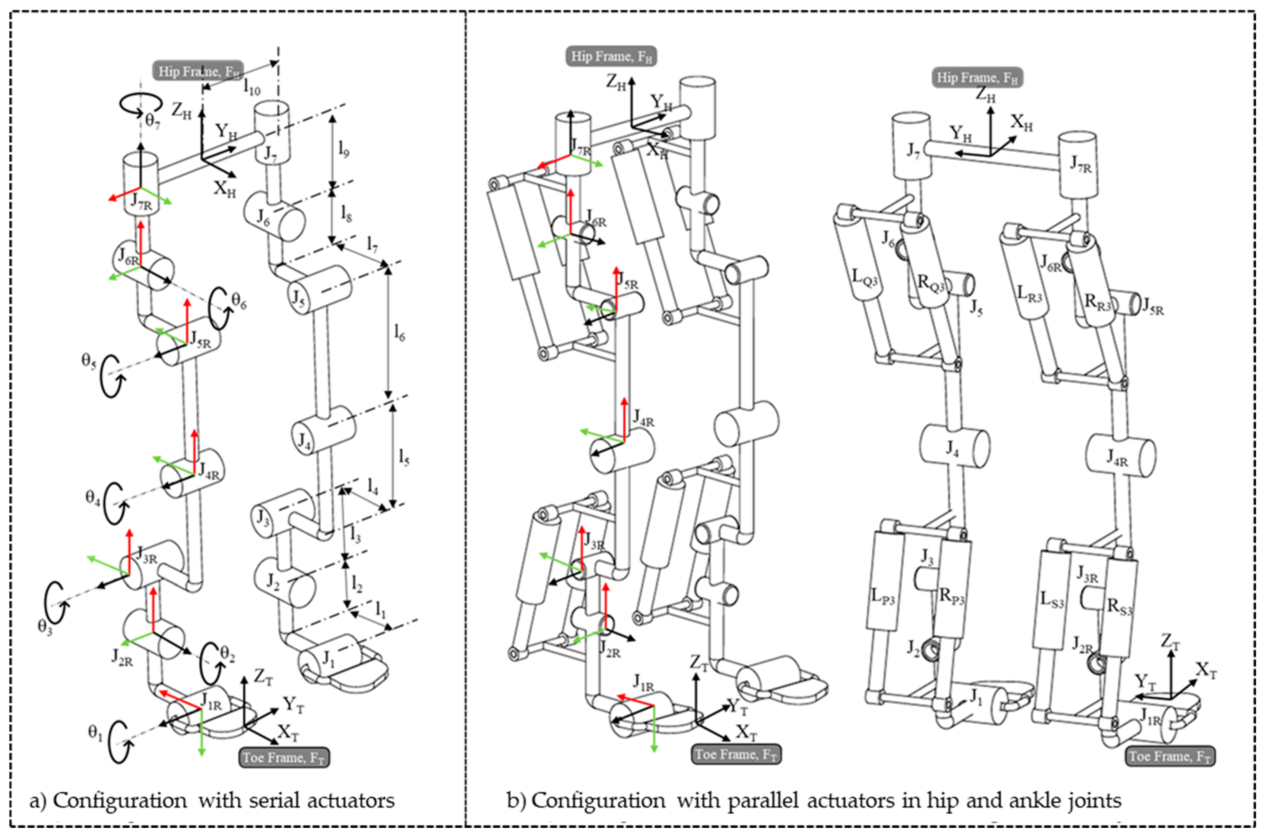
2. Methodology
- FT—Frame representing the toe link
- FH—Frame representing the hip link
- J1 (toe pitch joint): Provides pitch motion at the toe.
- J2 & J3 (ankle joints): Two revolute joints enabling independent roll and pitch movements at the ankle.
- J4 (knee pitch joint): A single revolute joint allowing pitch motion at the knee.
- J5, J6 & J7 (hip joints):
- ▪
- J5 & J6: Provide pitch and roll motion at the hip.
- ▪
- J7: Controls yaw motion at the hip.
2.1. Forward Kinematics
2.2. Theory on Inverse Kinematics
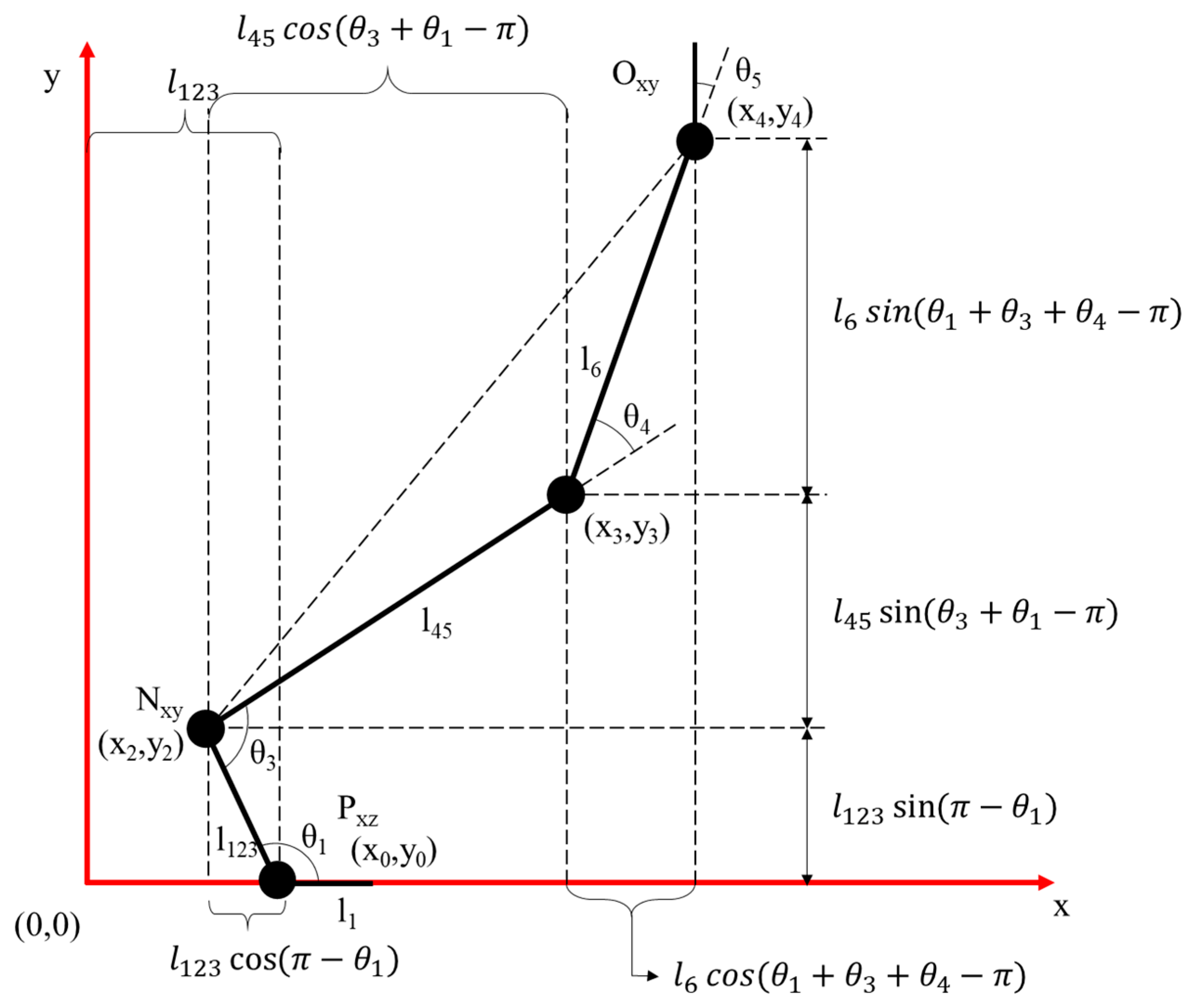
2.2.1. Inverse Kinematics in Sagittal Plane
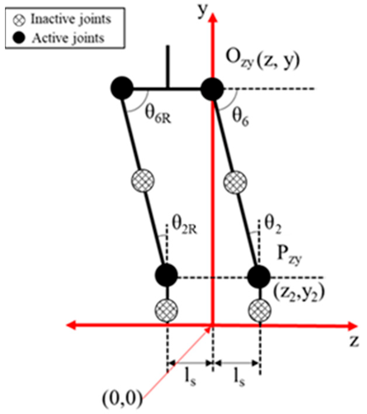
2.2.2. Inverse Kinematics in Frontal Plane
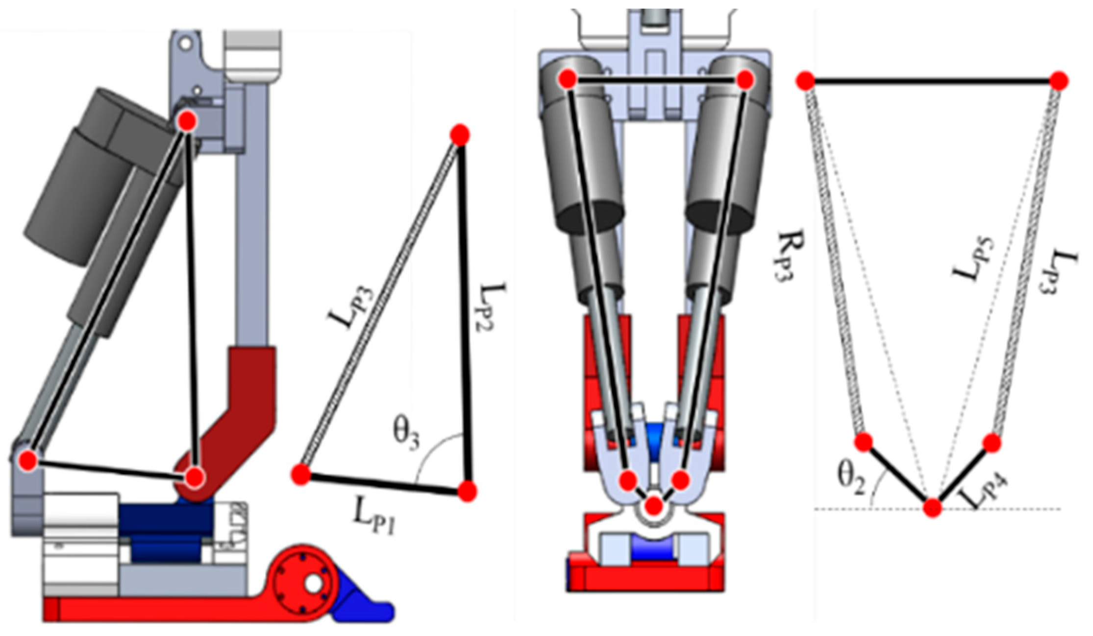
2.2.3. Inverse Kinematics for Linear Actuator Positions
3. Trajectory Planning
- Step length (s)—the forward distance moved in each step;
- Step time (T)—the duration of one complete step;
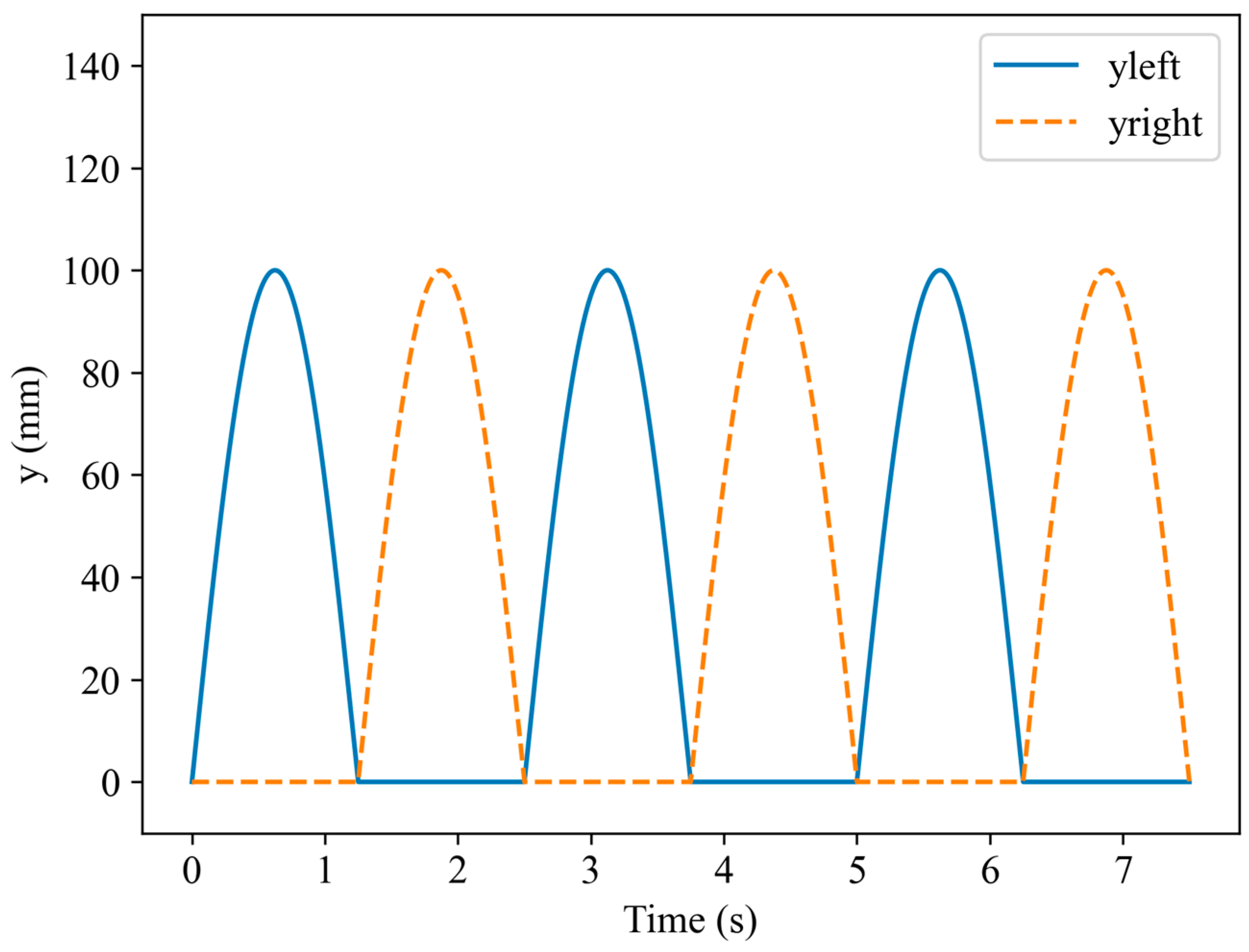
- Step height (sh)—the maximum vertical displacement of the foot during swing.
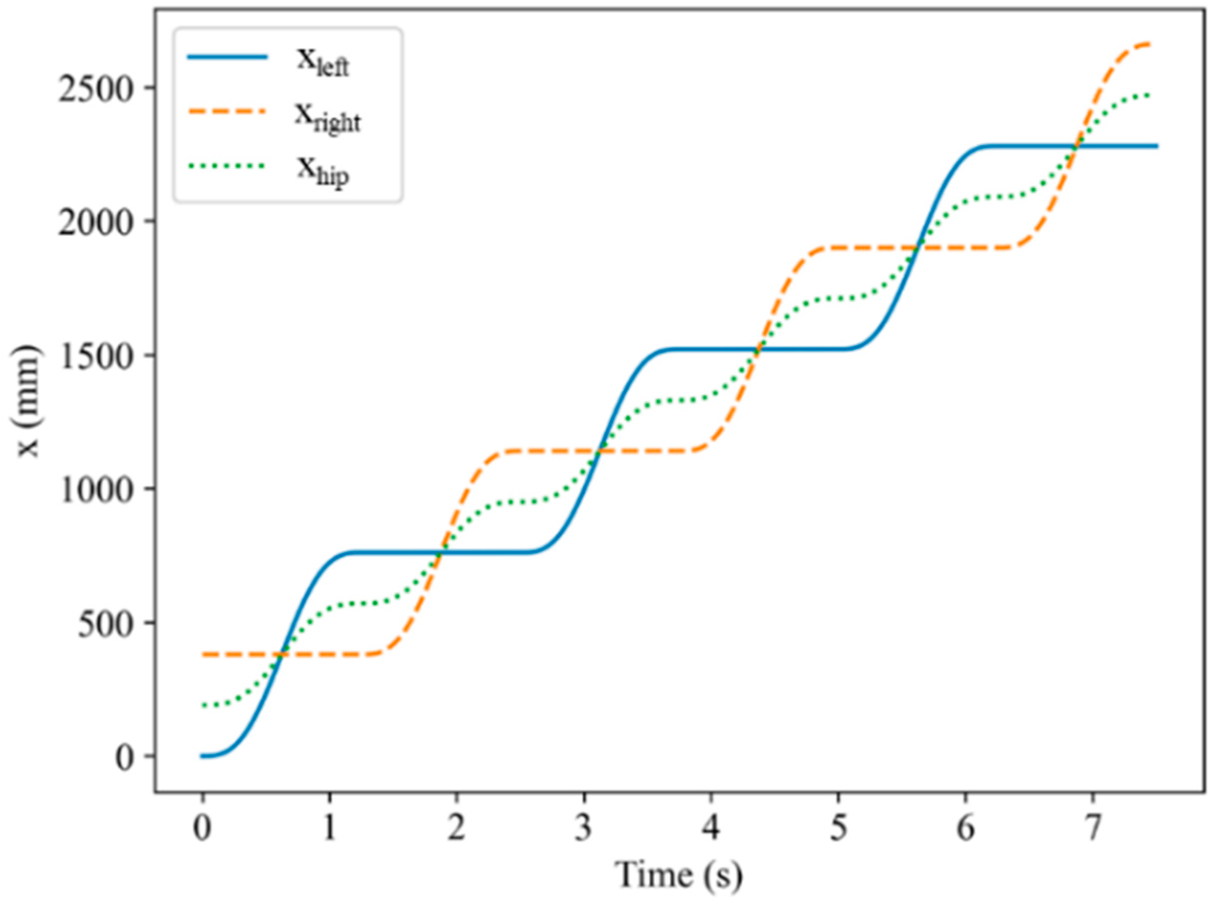
3.1. Deriving xleft and xright for Toe Frame
- During the stance phase, the foot is fixed: x = (n + 1)s;
- During the swing phase, the foot moves using the wave-based equation.
3.2. Deriving Yleft and Yright
3.3. Deriving Hip Trajectory
4. Results and Discussion
5. Conclusions
Author Contributions
Funding
Data Availability Statement
Acknowledgments
Conflicts of Interest
Abbreviations
| Symbol | Description |
| θ1 | Toe joint angle (left leg) |
| θ1R | Toe joint angle (right leg) |
| θ2 | Ankle roll joint angle (left leg) |
| θ2R | Ankle roll joint angle (right leg) |
| θ3 | Ankle pitch joint angle (left leg) |
| θ3R | Ankle pitch joint angle (right leg) |
| θ4 | Knee pitch joint angle (left leg) |
| θ4R | Knee pitch joint angle (right leg) |
| θ5 | Hip pitch joint angle (left leg) |
| θ5R | Hip pitch joint angle (right leg) |
| θ6 | Hip roll joint angle (left leg) |
| θ6R | Hip roll joint angle (right leg) |
| θ7 | Hip yaw joint angle (left leg) |
| θ7R | Hip yaw joint angle (right leg) |
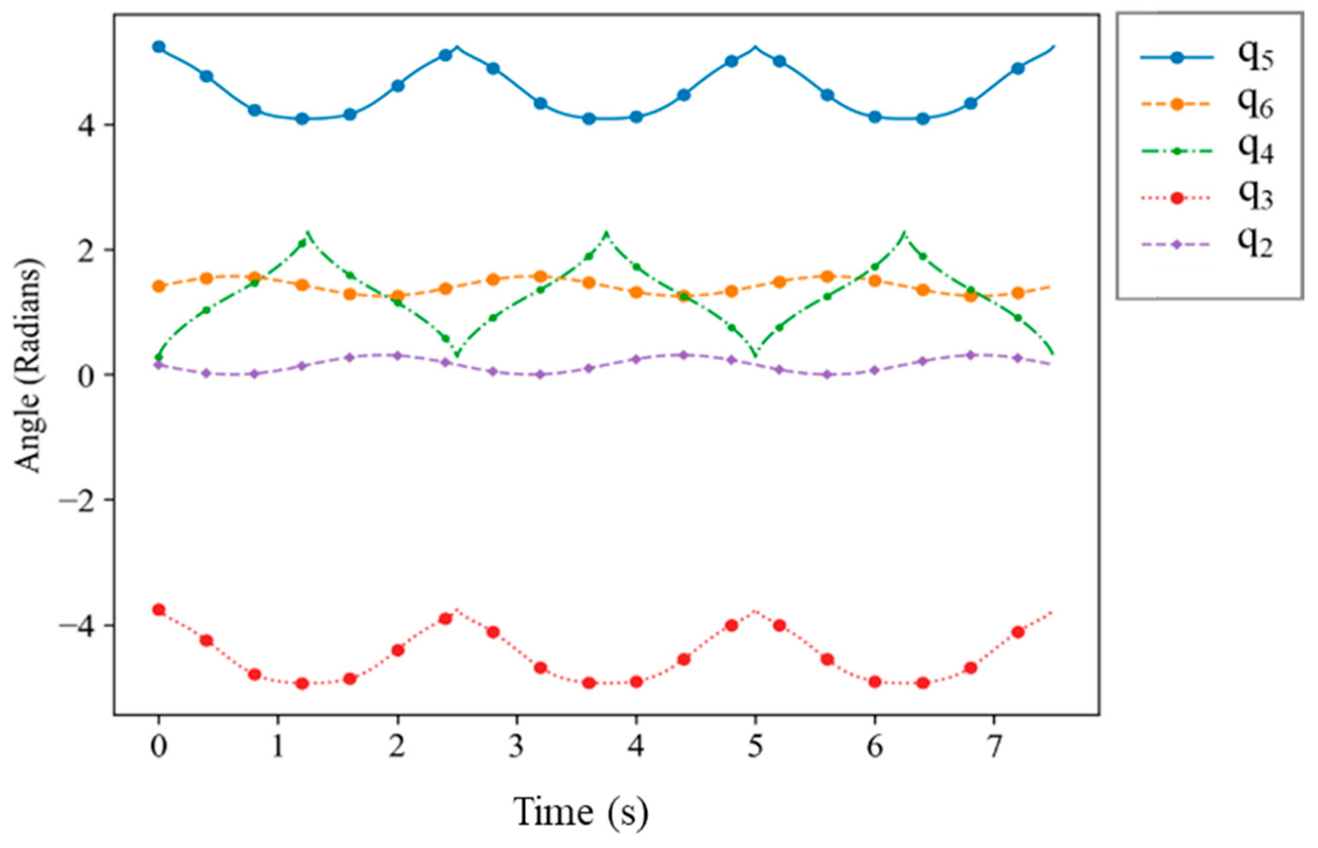
| q2 | Output at ankle roll joint (left leg) |
| q3 | Output at ankle pitch joint (left leg) |
| q4 | Output at knee pitch joint (left leg) |
| q5 | Output at hip pitch joint (left leg) |
| q6 | Output at hip roll joint (left leg) |
| q2R | Output at ankle roll joint (right leg) |
| q3R | Output at ankle pitch joint (right leg) |
| q4R | Output at knee pitch joint (right leg) |
| q5R | Output at hip pitch joint (right leg) |
| q6R | Output at hip roll joint (right leg) |
| l–l10 | Link lengths (various segments) |
| l45 | Combined link from hip to knee |
| ls | Lateral spacing between legs |
| LP3 | Length of the linear actuator on the left leg’s ankle joint—left-side actuator. |
| LP1, LP2, LP4, LP5, | Constant link lengths used in deriving the relationship between joint angle and actuator length for LP3. |
| RP3 | Length of the linear actuator on the left leg’s ankle joint—right-side actuator. |
| RP1, RP2, RP4, RP5, | Constant link lengths used in deriving the relationship between joint angle and actuator length for RP3. |
| LQ3 | Length of the linear actuator on the left leg’s hip joint—left-side actuator. |
| LQ1, LQ2, LQ4, LQ5, | Constant link lengths used in deriving the relationship between joint angle and actuator length for LQ3. |
| RQ3 | Length of the linear actuator on the left leg’s hip joint—right-side actuator. |
| RQ1, RQ2, RQ4, RQ5, | Constant link lengths used in deriving the relationship between joint angle and actuator length for RQ3. |
| LR3 | Length of the linear actuator on the right leg’s hip joint—left-side actuator. |
| LR1, LR2, LR4, LR5, | Constant link lengths used in deriving the relationship between joint angle and actuator length for LR3. |
| RR3 | Length of the linear actuator on the left leg’s hip joint—right-side actuator. |
| RR1, RR2, RR4, RR5, | Constant link lengths used in deriving the relationship between joint angle and actuator length for RR3. |
| LS3 | Length of the linear actuator on the left leg’s ankle joint—left-side actuator. |
| LS1, LS2, LS4, LS5, | Constant link lengths used in deriving the relationship between joint angle and actuator length for LS3. |
| RS3 | Length of the linear actuator on the left leg’s ankle joint—right-side actuator. |
| RS1, RS2, RS4, RS5, | Constant link lengths used in deriving the relationship between joint angle and actuator length for RS3. |
| S | Step length |
| T | Step time |
| Sh | The maximum vertical displacement |
| T | Current time instance |
| N | Current step |
References
- Dafarra, S.; Romualdi, G.; Pucci, D. Dynamic Complementarity Conditions and Whole-Body Trajectory Optimization for Humanoid Robot Locomotion. IEEE Trans. Robot. 2022, 38, 3414–3433. [Google Scholar] [CrossRef]
- Mikolajczyk, T.; Mikołajewska, E.; Al-Shuka, H.F.N.; Malinowski, T.; Kłodowski, A.; Pimenov, D.Y.; Paczkowski, T.; Hu, F.; Giasin, K.; Mikołajewski, D.; et al. Recent Advances in Bipedal Walking Robots: Review of Gait, Drive, Sensors and Control Systems. Sensors 2022, 22, 4440. [Google Scholar] [CrossRef]
- Sugano, S.; Shirai, Y. Robot Design and Environment Design—Waseda Robot-House Project. In Proceedings of the 2006 IEEE SICE-ICASE International Joint Conference, Busan, Republic of Korea, 18–21 October 2006; pp. I-31–I-34. [Google Scholar]
- Kato, I.; Ohteru, S.; Shirai, K.; Narita, S.; Sugano, S.; Matsushima, T.; Kobayashi, T.; Fujisawa, E. Sensing in Robotic Control The Robot Musician ‘WABOT-2’. Robotics 1987, 3, 143–155. [Google Scholar] [CrossRef]
- Hirose, M.; Ogawa, K. Honda Humanoid Robots Development. Philos. Trans. R. Soc. A Math. Phys. Eng. Sci. 2007, 365, 11–19. [Google Scholar] [CrossRef]
- Hashimoto, S.; Narita, S.; Kasahara, H.; Shirai, K.; Kobayashi, T.; Takanishi, A.; Sugano, S.; Yamaguchi, J.; Sawada, H.; Takanobu, H.; et al. Humanoid Robots in Waseda University—Hadaly-2 and WABIAN. Auton. Robots 2002, 12, 25–38. [Google Scholar] [CrossRef]
- Shirata, S.; Konno, A.; Uchiyama, M. Design and Evaluation of a Gravity Compensation Mechanism for a Humanoid Robot. In Proceedings of the 2007 IEEE/RSJ International Conference on Intelligent Robots and Systems, San Diego, CA, USA, 29 October–2 November 2007; pp. 3635–3640. [Google Scholar]
- Reher, J.; Ma, W.-L.; Ames, A.D. Dynamic Walking with Compliance on a Cassie Bipedal Robot. In Proceedings of the 2019 IEEE 18th European Control Conference (ECC), Naples, Italy, 25–28 June 2019; pp. 2589–2595. [Google Scholar]
- Gong, Y.; Hartley, R.; Da, X.; Hereid, A.; Harib, O.; Huang, J.-K.; Grizzle, J. Feedback Control of a Cassie Bipedal Robot: Walking, Standing, and Riding a Segway. In Proceedings of the 2019 IEEE American Control Conference (ACC), Philadelphia, PA, USA, 10–12 July 2019; pp. 4559–4566. [Google Scholar]
- Badri-Spröwitz, A.; Aghamaleki Sarvestani, A.; Sitti, M.; Daley, M.A. BirdBot Achieves Energy-Efficient Gait with Minimal Control Using Avian-Inspired Leg Clutching. Sci. Robot. 2022, 7, eabg4055. [Google Scholar] [CrossRef] [PubMed]
- Shigemi, S. ASIMO and Humanoid Robot Research at Honda; Springer: Dordrecht, The Netherlands, 2018; ISBN 9789400760462. [Google Scholar]
- Nagasaka, K. Sony QRIO. In Humanoid Robotics: A Reference; Springer: Dordrecht, The Netherlands, 2019; pp. 187–200. [Google Scholar] [CrossRef]
- Kuwayama, K.; Kato, S.; Seki, H.; Yamakita, T.; Itoh, H. Motion Control for Humanoid Robots Based on the Concept Learning. In Proceedings of the 2003 IEEE International Symposium on Micromechatronics and Human Science (IEEE Cat. No.03TH8717), Nagoya, Japan, 19–22 October 2003; pp. 259–263. [Google Scholar]
- Heo, J.-W.; Lee, I.-H.; Oh, J.-H. Development of Humanoid Robots in HUBO Laboratory, KAIST. J. Robot. Soc. Jpn. 2012, 30, 367–371. [Google Scholar] [CrossRef]
- Park, I.-W.; Kim, J.-Y.; Lee, J.; Oh, J.-H. Mechanical Design of the Humanoid Robot Platform, HUBO. Adv. Robot. 2007, 21, 1305–1322. [Google Scholar] [CrossRef]
- Catalano, M.G.; Frizza, I.; Morandi, C.; Grioli, G.; Ayusawa, K.; Ito, T.; Venture, G. HRP-4 Walks on Soft Feet. IEEE Robot. Autom. Lett. 2021, 6, 470–477. [Google Scholar] [CrossRef]
- Ogura, Y.; Aikawa, H.; Shimomura, K.; Kondo, H.; Morishima, A.; Lim, H.-O.; Takanishi, A. Development of a New Humanoid Robot WABIAN-2. In Proceedings of the 2006 IEEE International Conference on Robotics and Automation, ICRA 2006, Orlando, FL, USA, 15–19 May 2006; pp. 76–81. [Google Scholar]
- Ogura, Y.; Shimomura, K.; Kondo, A.; Morishima, A.; Okubo, T.; Momoki, S.; Lim, H.O.; Takanishi, A. Human-like Walking with Knee Stretched, Heel-Contact and Toe-off Motion by a Humanoid Robot. In Proceedings of the 2006 IEEE/RSJ International Conference on Intelligent Robots and Systems, Beijing, China, 9–15 October 2006; pp. 3976–3981. [Google Scholar]
- Hoffman, E.M.; Kothakota, S.; Moreno, A.; Curti, A.; Miguel, N.; Marchionni, L.; Kishor Kothakota, S.; Moreno, A.R. Whole-Body Kinematics Modeling in Presence of Closed-Linkages: Application to the Kangaroo Biped Robot. In Proceedings of the International Conference on Robotics and Automation (ICRA) 2022, Workshop on “New frontiers of parallel robotics”, Philadelphia, PA, USA, 23–27 May 2022. [Google Scholar]
- Lohmeier, S.; Buschmann, T.; Ulbrich, H. System Design and Control of Anthropomorphic Walking Robot LOLA. IEEE/ASME Trans. Mechatron. 2009, 14, 658–666. [Google Scholar] [CrossRef]
- Tellez, R.; Ferro, F.; Garcia, S.; Gomez, E.; Jorge, E.; Mora, D.; Pinyol, D.; Oliver, J.; Torres, O.; Velazquez, J.; et al. Reem-B: An Autonomous Lightweight Human-Size Humanoid Robot. In Proceedings of the Humanoids 2008—8th IEEE-RAS International Conference on Humanoid Robots, Daejeon, Republic of Korea, 1–3 December 2008; pp. 462–468. [Google Scholar]
- Shamsuddin, S.; Ismail, L.I.; Yussof, H.; Ismarrubie Zahari, N.; Bahari, S.; Hashim, H.; Jaffar, A. Humanoid Robot NAO: Review of Control and Motion Exploration. In Proceedings of the 2011 IEEE International Conference on Control System, Computing and Engineering, Penang, Malaysia, 25–27 November 2011; pp. 511–516. [Google Scholar]
- Zheng, Y.F.; Wang, H.; Li, S.; Liu, Y.; Orin, D.; Sohn, K.; Oh, P. Humanoid Robots Walking on Grass, Sands and Rocks. In Proceedings of the 2013 IEEE Conference on Technologies for Practical Robot Applications (TePRA), Woburn, MA, USA, 22–23 April 2013; pp. 1–6. [Google Scholar]
- Aller, F.; Harant, M.; Sontag, S.; Millard, M.; Mombaur, K. I3SA: The Increased Step Size Stability Assessment Benchmark and Its Application to the Humanoid Robot REEM-C. In Proceedings of the 2021 IEEE/RSJ International Conference on Intelligent Robots and Systems (IROS), Prague, Czech Republic, 27 September–1 October 2021; pp. 5357–5363. [Google Scholar]
- Lanari, L.; Hutchinson, S.; Marchionni, L. Boundedness Issues in Planning of Locomotion Trajectories for Biped Robots. In Proceedings of the 2014 IEEE-RAS International Conference on Humanoid Robots, Madrid, Spain, 18–20 November 2014; pp. 951–958. [Google Scholar]
- Kuindersma, S.; Deits, R.; Fallon, M.; Valenzuela, A.; Dai, H.; Permenter, F.; Koolen, T.; Marion, P.; Tedrake, R. Optimization-Based Locomotion Planning, Estimation, and Control Design for the Atlas Humanoid Robot. Auton. Robots 2016, 40, 429–455. [Google Scholar] [CrossRef]
- Hyon, S.-H.; Suewaka, D.; Torii, Y.; Oku, N. Design and Experimental Evaluation of a Fast Torque-Controlled Hydraulic Humanoid Robot. IEEE/ASME Trans. Mechatron. 2017, 22, 623–634. [Google Scholar] [CrossRef]
- Arena, P.; Patané, L.; Spinosa, A.G. A New Embodied Motor-Neuron Architecture. IEEE Trans. Control Syst. Technol. 2021, 30, 2212–2219. [Google Scholar] [CrossRef]
- Arena, P.; Patané, L.; Spinosa, A.G. A Nullcline-Based Control Strategy for PWL-Shaped Oscillators. Nonlinear Dyn. 2019, 97, 1587–1603. [Google Scholar] [CrossRef]
- Pandilov, Z.; Dukovski, V. Comparison of the Characteristics Between Serial and Parallel Robots. Fascicule 2014, 1, 2067–3809. [Google Scholar]
- Kucuk, S.; Gungor, B.D. Inverse Kinematics Solution of a New Hybrid Robot Manipulator Proposed for Medical Purposes. In Proceedings of the 2016 IEEE Medical Technologies National Congress (TIPTEKNO), Antalya, Turkey, 27–29 October 2016; pp. 1–4. [Google Scholar]
- Sun, P.; Li, Y.; Wang, Z.; Chen, K.; Chen, B.; Zeng, X.; Zhao, J.; Yue, Y. Inverse Displacement Analysis of a Novel Hybrid Humanoid Robotic Arm. Mech. Mach. Theory 2020, 147, 103743. [Google Scholar] [CrossRef]
- Briot, S.; Bonev, I.A. Are Parallel Robots More Accurate than Serial Robots? Trans. Can. Soc. Mech. Eng. 2007, 31, 445–455. [Google Scholar] [CrossRef]
- Nzue, R.-M.A.; Brethé, J.-F.; Vasselin, E.; Lefebvre, D. Comparison of Serial and Parallel Robot Repeatability Based on Different Performance Criteria. Mech. Mach. Theory 2013, 61, 136–155. [Google Scholar] [CrossRef]
- Vodovozov, V.; Raud, Z.; Petlenkov, E. Intelligent Control of Robots with Minimal Power Consumption in Pick-and-Place Operations. Energies 2023, 16, 7418. [Google Scholar] [CrossRef]
- Roberts, D.; Quacinella, J.; Kim, J.H. Energy Expenditure of a Biped Walking Robot: Instantaneous and Degree-of-Freedom-Based Instrumentation with Human Gait Implications. Robotica 2017, 35, 1054–1071. [Google Scholar] [CrossRef]
- Collins, S.H.; Ruina, A.; Tedrake, R.; Wisse, M. Efficient Bipedal Robots Based on Passive-Dynamic Walkers. Science 2005, 307, 1082–1085. [Google Scholar] [CrossRef]
- Inman, V.T.; Ralston, H.J.; Todd, F. Human Walking; Williams & Wilkins: Baltimore, MD, USA, 1981. [Google Scholar] [CrossRef]
- Perry, J.; Burnfield, J.M. Gait Analysis: Normal and Pathological Function, 2nd ed.; SLACK Incorporated: Thorofare, NJ, USA, 2010. [Google Scholar] [PubMed Central]
- Kajita, S.; Kanehiro, F.; Kaneko, K.; Fujiwara, K.; Harada, K.; Yokoi, K.; Hirukawa, H. Biped Walking Pattern Generation by Using Preview Control of Zero-Moment Point. In Proceedings of the 2003 IEEE International Conference on Robotics and Automation (ICRA), Taipei, Taiwan, 14–19 September 2003; pp. 1620–1626. [Google Scholar] [CrossRef]


| S. No | Parameters | Values |
|---|---|---|
| 1 | Step length | 760 mm |
| 2 | Step height | 100 mm |
| 3 | Step time | 2.5 s |
| 4 | Distance between two centres of the foot in ‘z’ axis | 93.96 mm |
| S. No | Joint | Maximum Instantaneous Power (W) | ||
|---|---|---|---|---|
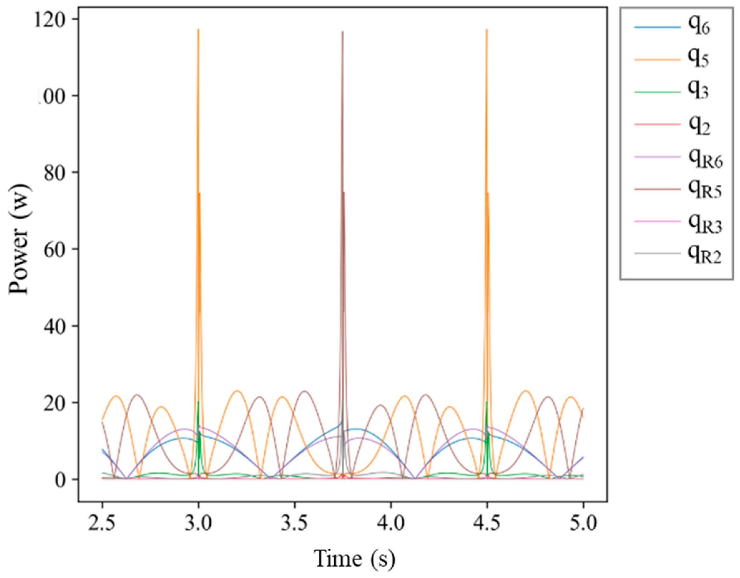
| 1 | Left Leg | Hip roll | q6 | 15.26021 |
| 2 | Hip pitch | q5 | 117.245 | |
| 3 | Ankle pitch | q3 | 20.26243 | |
| 4 | Ankle roll | q2 | 1.395065 | |
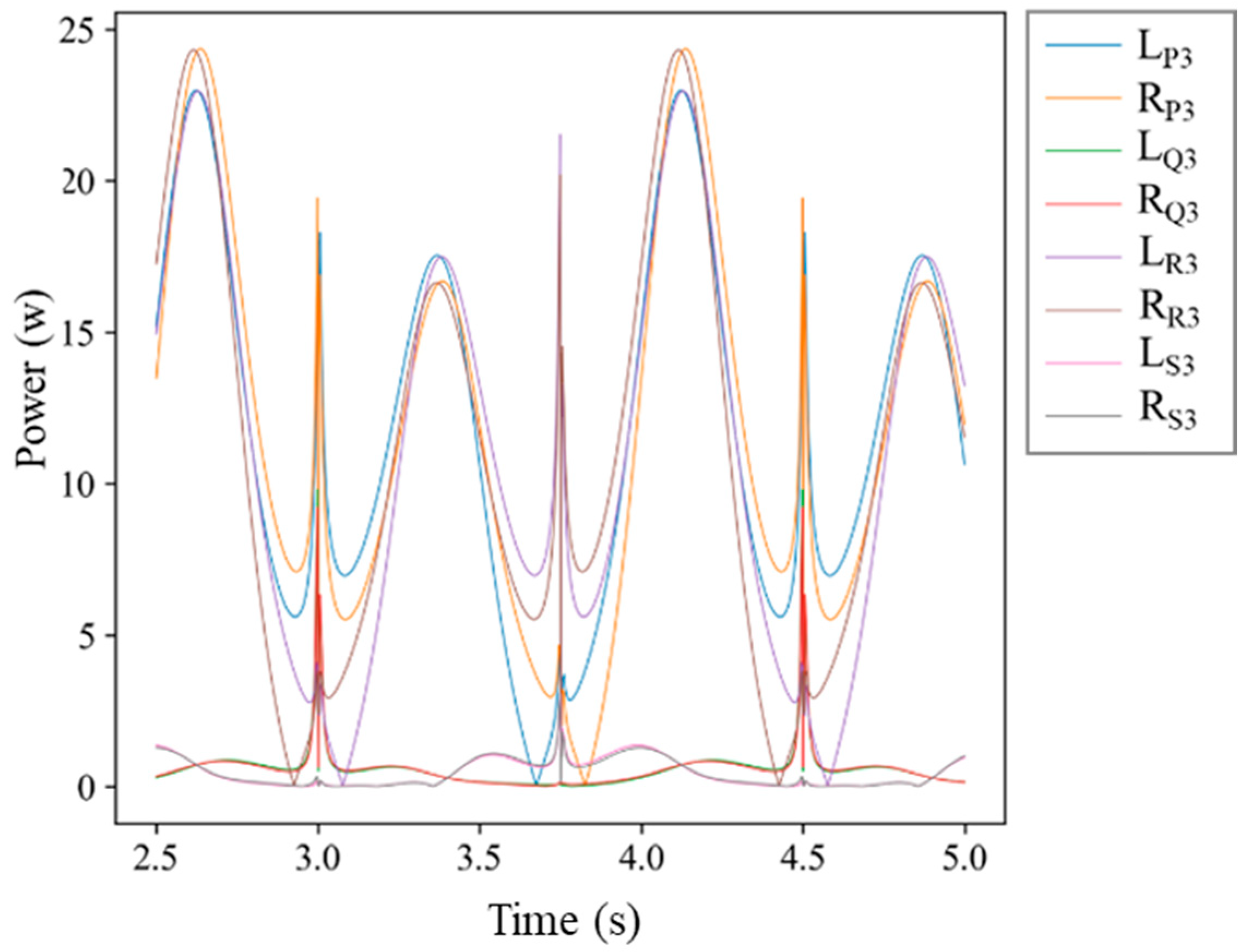
| 5 | Hip parallel | Lq3 | 22.98631 | |
| 6 | Rq3 | 24.3601 | ||
| 7 | Ankle parallel | Lp3 | 9.795821 | |
| 8 | Rp3 | 9.206407 | ||
| 9 | Right Leg | Hip roll | q6r | 13.96714 |
| 10 | Hip pitch | q5r | 116.6731 | |
| 11 | Ankle pitch | q3r | 20.49206 | |
| 12 | Ankle roll | q2r | 0.722933 | |
| 13 | Hip parallel | Lr3 | 22.95801 | |
| 14 | Rr3 | 24.32176 | ||
| 15 | Ankle parallel | Ls3 | 3.036088 | |
| 16 | Rs3 | 3.066172 | ||
Disclaimer/Publisher’s Note: The statements, opinions and data contained in all publications are solely those of the individual author(s) and contributor(s) and not of MDPI and/or the editor(s). MDPI and/or the editor(s) disclaim responsibility for any injury to people or property resulting from any ideas, methods, instructions or products referred to in the content. |
© 2025 by the authors. Licensee MDPI, Basel, Switzerland. This article is an open access article distributed under the terms and conditions of the Creative Commons Attribution (CC BY) license (https://creativecommons.org/licenses/by/4.0/).
Share and Cite
Manoharan, P.; Palanisamy, K. Energy-Efficient Bipedal Locomotion Through Parallel Actuation of Hip and Ankle Joints. Symmetry 2025, 17, 1110. https://doi.org/10.3390/sym17071110
Manoharan P, Palanisamy K. Energy-Efficient Bipedal Locomotion Through Parallel Actuation of Hip and Ankle Joints. Symmetry. 2025; 17(7):1110. https://doi.org/10.3390/sym17071110
Chicago/Turabian StyleManoharan, Prabhu, and Karthikeyan Palanisamy. 2025. "Energy-Efficient Bipedal Locomotion Through Parallel Actuation of Hip and Ankle Joints" Symmetry 17, no. 7: 1110. https://doi.org/10.3390/sym17071110
APA StyleManoharan, P., & Palanisamy, K. (2025). Energy-Efficient Bipedal Locomotion Through Parallel Actuation of Hip and Ankle Joints. Symmetry, 17(7), 1110. https://doi.org/10.3390/sym17071110