Attention-Based Mask R-CNN Enhancement for Infrared Image Target Segmentation

Abstract

Image segmentation is an important method in the field of image processing, while infrared (IR) image segmentation is one of the challenges in this field due to the unique characteristics of IR data. Infrared imaging utilizes the infrared radiation emitted by objects to produce images, which can supplement the performance of visible-light images under adverse lighting conditions to some extent. However, the low spatial resolution and limited texture details in IR images hinder the achievement of high-precision segmentation. To address these issues, an attention mechanism based on symmetrical cross-channel interaction—motivated by symmetry principles in computer vision—was integrated into a Mask Region-Based Convolutional Neural Network (Mask R-CNN) framework. A Bottleneck-enhanced Squeeze-and-Attention (BNSA) module was incorporated into the backbone network, and novel loss functions were designed for both the bounding box (Bbox) regression and mask prediction branches to enhance segmentation performance. Furthermore, a dedicated infrared image dataset was constructed to validate the proposed method. The experimental results demonstrate that the optimized model achieves higher segmentation accuracy and better segmentation performance compared to the original network and other mainstream segmentation models on our dataset, demonstrating how symmetrical design principles can effectively improve complex vision tasks.

1. Introduction

Image segmentation is one of the most important methods in the field of image processing. It can classify the pixels of an input image and separate the target from the background. It has been widely used in various fields such as disease diagnosis [1], agricultural production [2], intelligent driving [3] and defect detection [4].

Usually, target segmentation methods are divided into traditional image segmentation methods and image segmentation methods based on deep learning. Traditional image segmentation methods include matched filtering, edge detection, threshold segmentation, active contour model methods [5], and so on. In some special cases, they can achieve good segmentation results. However, traditional segmentation algorithms are limited to surface features of the image and cannot fully exploit deeper semantic information. This limitation makes them less effective in today’s increasingly complex image backgrounds. With the continuous development of deep learning methods, neural networks are applied in the field of image segmentation gradually. They can address the limitations of traditional image segmentation techniques. In particular, convolutional neural networks have been widely used. In 2014, Ross Girshick introduced the R-CNN [6] based on convolutional neural networks, which laid a solid foundation for the development of convolutional neural networks in the field of object detection. Later in 2015, Girshick R proposed Fast R-CNN [7] to address the significant time consumption issues of R-CNN. By optimizing the way of extracting features from candidate regions in R-CNN, Fast R-CNN improved the running efficiency of the overall model to some extent. In 2016, Faster R-CNN [8] was proposed by Shaoqing Ren. Its novelty lies in the design of the Region Proposal Network (RPN) to address the significant time burden caused by selective searching. Soon after, Mask R-CNN [9] emerged based on Faster R-CNN. Mask R-CNN utilizes ROI Align instead of ROI pooling to improve detection speed. Additionally, it incorporates a dedicated mask branch in the output stage, enhancing its suitability for instance segmentation tasks.

In 2019, Bolya D et al. [10] introduced Yolact, an efficient segmentation network that adopts a parallel mask branch to perform detection and generate prototype masks simultaneously. Each instance is assigned a set of mask coefficients which are linearly combined with the prototypes to produce the final instance masks. Building on this idea, Chen H proposed BlendMask [11] in 2020, which merges concepts from both Mask R-CNN and Yolact. By appending a mask branch to the FCOS [12] framework and incorporating a Blender module that fuses instance-level and semantic-level features, BlendMask achieves improved segmentation accuracy and flexibility through the integration of top–down and bottom–up information. A similar paradigm is followed by CondInst [13], which dynamically generates a unique mask head for each instance and couples it with shared global mask features to yield accurate instance masks. In the same year, Wang X et al. proposed Solo [14], a different segmentation approach that directly predicts object categories based on spatial position and shape, eliminating the need for bounding box proposals. Its improved variant, Solov2 [15], further separates the mask head into kernel and feature branches, allowing for dynamic mask prediction and incorporating Matrix NMS to accelerate inference. In 2021, BoxInst [16] was introduced as a weakly supervised extension of CondInst. It employs a novel loss formulation that enables training without relying on pixel-level mask annotations, offering a more annotation-efficient alternative without modifying the network structure. Developed more recently, SparseInst [17] (2022) adopts a sparse activation-based strategy, leveraging a compact set of instance activation maps to perform instance segmentation more efficiently. By circumventing the traditional NMS process, SparseInst improves overall speed while maintaining segmentation quality.

Infrared image segmentation is a challenging task in image processing. Infrared imaging utilizes the infrared radiation emitted by objects to produce images. It is less affected by lighting conditions and exhibits stronger anti-interference capabilities. In certain cases, infrared images can complement the performance of visible-light images under harsh lighting conditions. However, due to the relatively low overall resolution of infrared images, it is difficult to obtain highly precise infrared image details. Therefore, utilizing neural networks for infrared image segmentation poses certain challenges. Currently, a mainstream approach to handling the segmentation of infrared images is to combine the feature information from both infrared and RGB images. Ha Q et al. [18] proposed MFNet, which utilizes an encoder–decoder architecture to process image data. The encoder employs a CNN network with dilated convolutions for feature extraction. Additionally, a short-cut block is designed to combine the feature maps of both IR and RGB images in the decoder. Inspired by MFNet, Sun Y et al. [19] adopted a similar architecture and chose ResNet as the feature extraction module for the encoder. They also designed an Upception module in the decoder to restore the image resolution. The experimental results demonstrated that this method achieved better segmentation accuracy and faster processing speed compared to MFNet. Subsequently, Shivakumar [20] optimized the existing methods for RGB-T image calibration and designed a dual-path CNN structure to integrate the features of RGB-T images, further improving the algorithm’s processing speed. However, the aforementioned methods do not address the issue of not utilizing infrared image feature information in RGB-T segmentation fully. Meanwhile, the problem of the inability to obtain clear visible images under harsh conditions remains unresolved. They also cannot reduce the additional time required to perform operations such as image alignment in the preprocessing stage.

In recent years, deep learning-based infrared image segmentation has achieved notable progress, driven by continuous improvements in neural network architectures. A range of innovative methods have been proposed to tackle the challenges posed by the inherent fuzziness of infrared features. For instance, Xiong H et al. [21] introduced a Multi-level Attention Module (MAM) to strengthen intra-class feature representation using contextual cues, while their CMCM algorithm was designed to suppress inter-class interference. To further mitigate edge blurring in thermal imagery, they implemented a multi-level edge enhancement strategy. However, this approach showed limited effectiveness when dealing with small-scale infrared targets. Ren S et al. [22] focused on improving small-object segmentation by fusing low-level details with high-level semantic information. They also developed an edge enhancement technique based on explicit modeling to compensate for detail loss during feature extraction. From a broader perspective, Junwei Hu et al. [23] argued that segmentation should not be restricted to isolated object regions. They introduced Prior Scene Understanding (PSU) into their SAPN network, enabling global context modeling. While this approach reduced the influence of background variability, it did not fully resolve the issue of target–background boundary ambiguity. To further improve accuracy without excessive computational cost, Yu J et al. [24] enhanced the U-Net [25] architecture using a hierarchical-split depth-wise separable convolution block, along with a decoupled approach to convolution and batch normalization layers. This design offered a better trade-off between performance and efficiency. Aiming to address information degradation during resolution changes, Jiuzhou W et al. [26] proposed DFA-Net, a deep feature aggregation network. By aggregating multi-level features and applying mean filtering to suppress noise, their model achieved improved segmentation performance in complex infrared scenes. Despite the progress of deep learning in infrared image segmentation, several key challenges remain unresolved: accurate segmentation under complex, multi-class IR backgrounds; effective feature representation in low-texture IR data; and unstable training and poor convergence due to imbalance in object–background regions. To address these issues, we propose a novel infrared segmentation framework built upon Mask R-CNN, incorporating three key innovations:

• A Bottleneck-enhanced Squeeze-and-Attention (BNSA) module is designed and integrated into the backbone network. Unlike prior works that adopt generic attention mechanisms, the proposed BNSA module fuses both global contextual dependencies and fine-grained local details while introducing a lightweight bottleneck structure to reduce computational overhead. This structure is specifically optimized for infrared characteristics, where edge clarity and background suppression are critical.
• Two compound loss functions are formulated to improve training stability and precision. First, Focal_SIoU Loss is constructed by combining the directional spatial IoU (SIoU) Loss with Focal Loss, aiming to balance foreground–background contributions and accelerate bounding box convergence—an aspect not previously explored in this combination. Second, MBCE_Dice_LS Loss is proposed to jointly leverage pixel-level (MBCE), region-level (Dice), and rank-based (Lovasz-Softmax) gradients in mask prediction. While each component exists independently in the literature, our combined formulation targets the unique imbalance and misclassification patterns common in IR segmentation.
• A dedicated IR segmentation dataset with four object classes (humans, cars, bicycles, UAVs) is built for evaluation. Unlike many prior datasets that focus on dual-modal fusion (e.g., RGB-T), our dataset emphasizes single-modality IR scenes with complex backgrounds and target occlusion.

These contributions go beyond simple component integration by tailoring architectural and loss function design specifically for the unique demands of infrared object segmentation. Extensive experiments demonstrate that our method outperforms both classical and state-of-the-art models in terms of accuracy, robustness, and small-target sensitivity.

2. Related Work

2.1. Self-Infrared Dataset Production

In the process of algorithm research in deep learning, datasets play a very important role. Whether it is model training optimization or algorithm performance evaluation, specific datasets are used. Currently, there are few publicly available infrared image datasets specifically designed for image segmentation that include the four classes of objects we require: humans, cars, bicycles, and UAVs. Therefore, we collected images using an infrared thermographic camera, annotated the targets, and created a dataset for subsequent research.

We used the LA6110 high-performance uncooled infrared focal plane array (IRFPA) camera to capture the images. After data annotation, enhancement, and cleaning, we obtained a total of 2760 images. Figure 1 displays some of the infrared images included in the dataset. These images generated by the infrared image detector are grayscale, and their size is 640 × 512. In addition to the segmentation targets we need, the images also contain interference such as buildings, vegetation, clouds, and other elements, which make background segmentation more complex. To further assess the generalization capability of our method, we also evaluate it on the publicly available FLIR thermal dataset.

2.2. Transfer Learning

Transfer learning has become a common strategy in deep learning to address the problem of limited training data and to enhance model generalization capabilities [27]. It involves leveraging models that have been pre-trained on large-scale public datasets, enabling more efficient training and faster convergence for new tasks. Instead of training a model from scratch, a pre-trained network serves as a starting point, which significantly reduces the computational cost and improves performance, even when the target dataset differs substantially from the source data. This flexibility makes transfer learning especially useful in domains where annotated data are scarce.

In our work, we adopted the Mask R-CNN model pre-trained on the COCO dataset as the base network. To maintain annotation consistency during training, we formatted our custom infrared dataset using the same COCO-style annotation scheme.

3. Method

3.1. Overview of Principle of Mask R-CNN Model

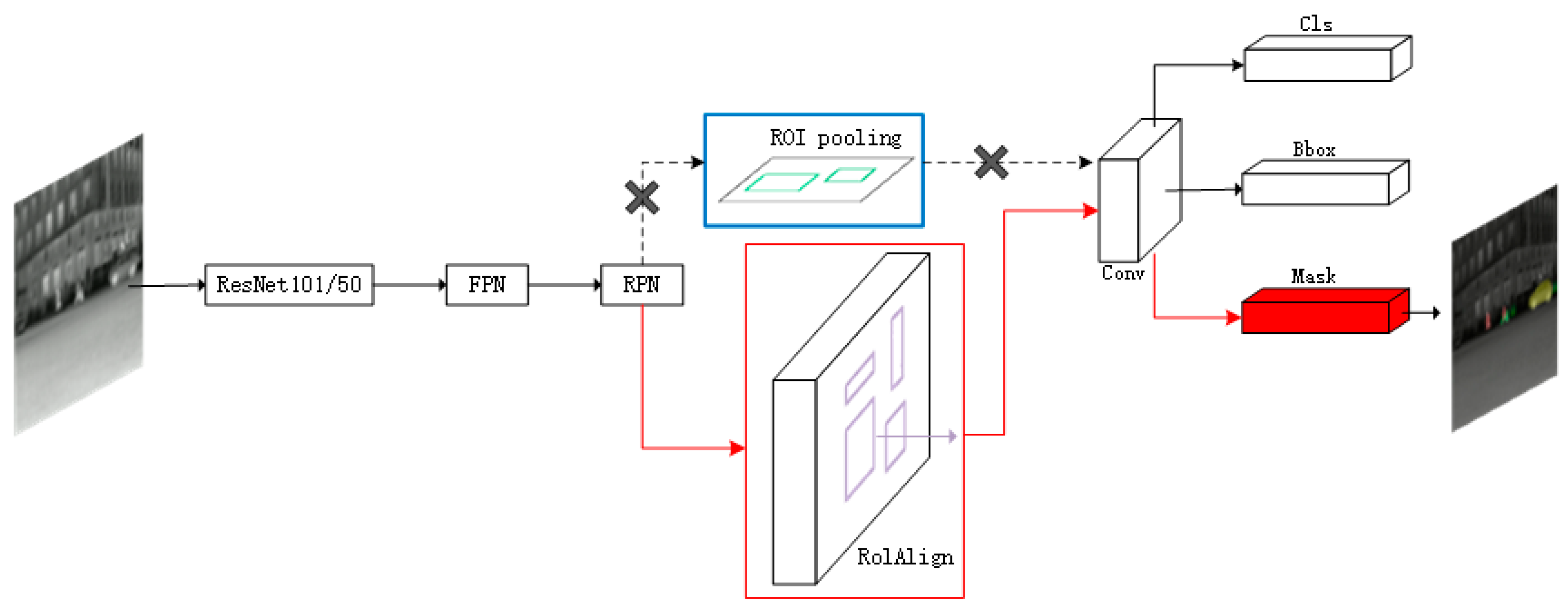
Mask R-CNN is a two-stage object detection network that is developed based on the Faster R-CNN network. The overall network structure is depicted in Figure 2, where the blue box represents the original structure of Faster R-CNN, and the red box represents the structure of Mask R-CNN. These two models share a similar structure; however, Mask R-CNN uses the RoI Align method, whereas Faster R-CNN adopts the ROI pooling technique. Additionally, Mask R-CNN introduces a parallel mask branch during the network’s output stage. In the following sections, we will discuss the main structure and principles of Mask R-CNN.

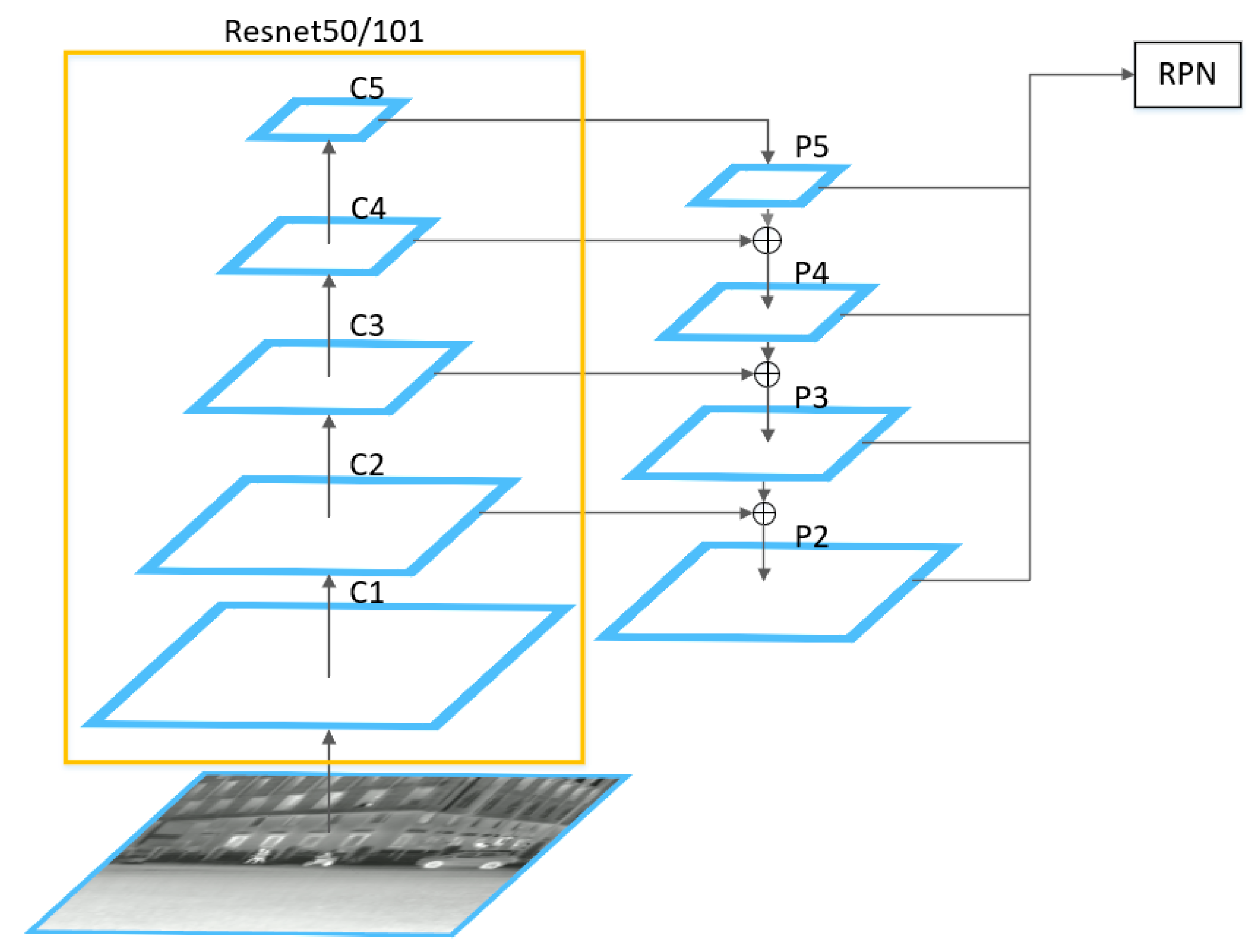
The backbone network of Mask R-CNN includes two parts: ResNet101/50 [28] and FPN. The former constructs a five-layer convolutional structure to generate feature maps of different scales for the input image, and the latter combines feature maps of different scales to construct a feature pyramid. Feature maps at different scales are progressively fused through a top–down sampling process, and output feature maps are generated based on the specific structure shown in Figure 3. The output feature maps are processed by a shared convolutional neural network in RPN to generate anchor boxes of various sizes. Subsequently, the classifier will provide probabilities for each anchor box, indicating whether it contains an object or background. Based on the scores of these probabilities, a certain number of anchor boxes are filtered out by the Proposal module. In addition, the Proposal module will also perform coordinate correction on the anchor boxes and remove regions that extend beyond the image boundaries or have excessively small sizes. Furthermore, it employs a technique called NMS to filter out duplicate candidate regions. Finally, it generates a set of candidate regions, known as ROI. A new method of ROI Align is used in Mask R-CNN. Since the ROIs output by the RPN may be of varying sizes, mapping them to the same dimensions can result in inconsistent receptive fields. To address this issue, Faster R-CNN introduces the RoI pooling method. However, RoI pooling involves rounding operations when resizing ROIs to a uniform size, which can lead to inaccuracies in the localization results. ROI Align uses bilinear interpolation to address the issues caused by rounding operations. This method allows for a more accurate determination of the mapped ROI coordinates, improving the overall detection accuracy of the network effectively.

The last part of the Mask R-CNN network is the prediction head, which consists of the class prediction part and Bbox prediction part from Faster R-CNN, along with the newly added mask prediction part. The class prediction part is responsible for determining the specific class probabilities of each target in the ROI. The total number of classes includes both the target classes and the background class. The Bbox prediction part is used to determine the final position of the detection boxes. It involves correcting the offset of the input position coordinates to ensure accurate localization. The added mask prediction part is responsible for obtaining the segmentation masks. It uses FCN to convert the input ROI into a fixed-size mask image of K × 28 × 28, where K represents the number of classes in the predicted input image. This enables precise segmentation of the target.

3.2. Improved Attention Mechanism Based on SA Module

The main purpose of the attention mechanism is to select the most salient information from image data [29]. The Squeeze-and-Attention (SA) module [30] is derived from the squeeze-and-excitation (SE) module [31]. It addresses the issue of pixel grouping in image segmentation by introducing attention convolutional channels for pixel-level predictions. This effectively enhances the performance of image segmentation.

Due to the nature of classical convolutional layers, their convolution operation on images only utilizes local information from each pixel to generate feature maps, without incorporating global image information. However, for a complete image, the different parts of the image often have correlations with each other. 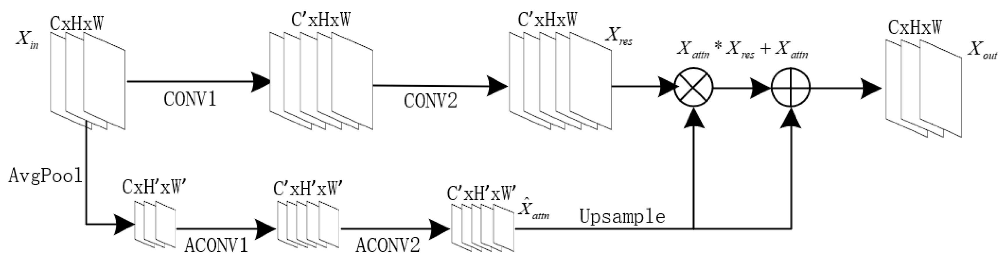This suggests that leveraging global contextual features to guide the learning process can offer more informative cues for image segmentation [32]. Therefore, the SA module considers reweighting through both global and local aspects. The specific structure of the SA module is shown in Figure 4.

The structure of the attention channel, as shown in Figure 4, can be represented by Equation (1):

$$X_{\mathrm{attn}}=Up(\sigma ({\widehat{X}}_{\mathrm{attn}}))=Up(\sigma (F_{attn}(Apool(X_{in});{\mathsf{\Omega }}_{attn})))$$

(1)

Among them, $Up(\cdot )$ is an upsampling function used to restore the size of the attention channel’s output feature map. $\sigma (\cdot )$ represents the Relu activation function. And ${\widehat{X}}_{attn}$ represents the output of the attention channel $F_{\mathrm{attn}}(\cdot )$. $F_{\mathrm{attn}}(\cdot )$ is the attention convolutional channel determined by ${\mathsf{\Omega }}_{attn}$, which consists of two convolutional layers. Additionally, an average pooling function $Apool(\cdot )$ is used to perform downsampling on the input feature map $X_{in}\in {\mathbb{R}}^{C\times H\times W}$. The SA module as a whole can be formulated as follows:

$$X_{out}=X_{attn}\ast X_{res}+X_{attn}$$

(2)

where $X_{out}\in {\mathbb{R}}^{C\times H\times W}$ represents the output feature map result, and $X_{res}$ is the output result of the main convolution channel, obtained from Equation (3):

$$X_{res}=F((X_{in});\mathsf{\Omega })$$

(3)

$F(\cdot )$ represents the main convolution channel determined by $\mathsf{\Omega }$, which consists of two convolutional layers.

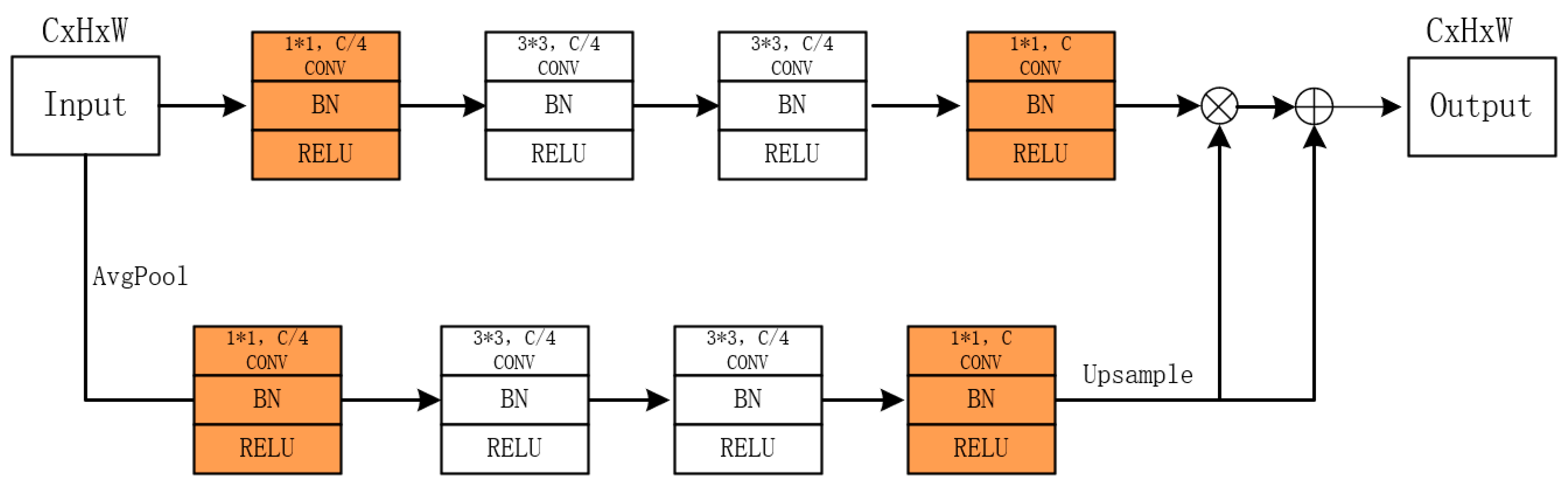
To further reduce the parameter burden of adding the attention module, we integrated the bottleneck [28] into the original SA module and named this new module BNSA. The bottleneck structure helps compress and optimize the feature representations within the SA module, resulting in more efficient utilization of parameters. As shown in the orange section of Figure 5, we added an additional 1 × 1 convolutional module before and after the main convolutional channels and attention convolutional channels within the original SA module. These modules serve to scale the number of channels, thereby reducing computational overhead while retaining essential information. Inspired by the form of the bottleneck in ResNet, we used a 1 × 1 convolution to scale the number of channels to 1/4 of the original convolution layer. The parameter quantity of a single convolution can be calculated using Equation (4):

$$params=n^2\ast c_{in}\ast c_{out}$$

(4)

where $n$ represents the size of the convolution kernel, and $c_{in}$ and $c_{out}$ represent the input and output channel numbers of the convolution layer, respectively. For the SA module that incorporates the bottleneck structure, the parameter count of the overall convolutional modules is significantly reduced. This greatly alleviates the computational burden of the model, resulting in more efficient model training and inference.

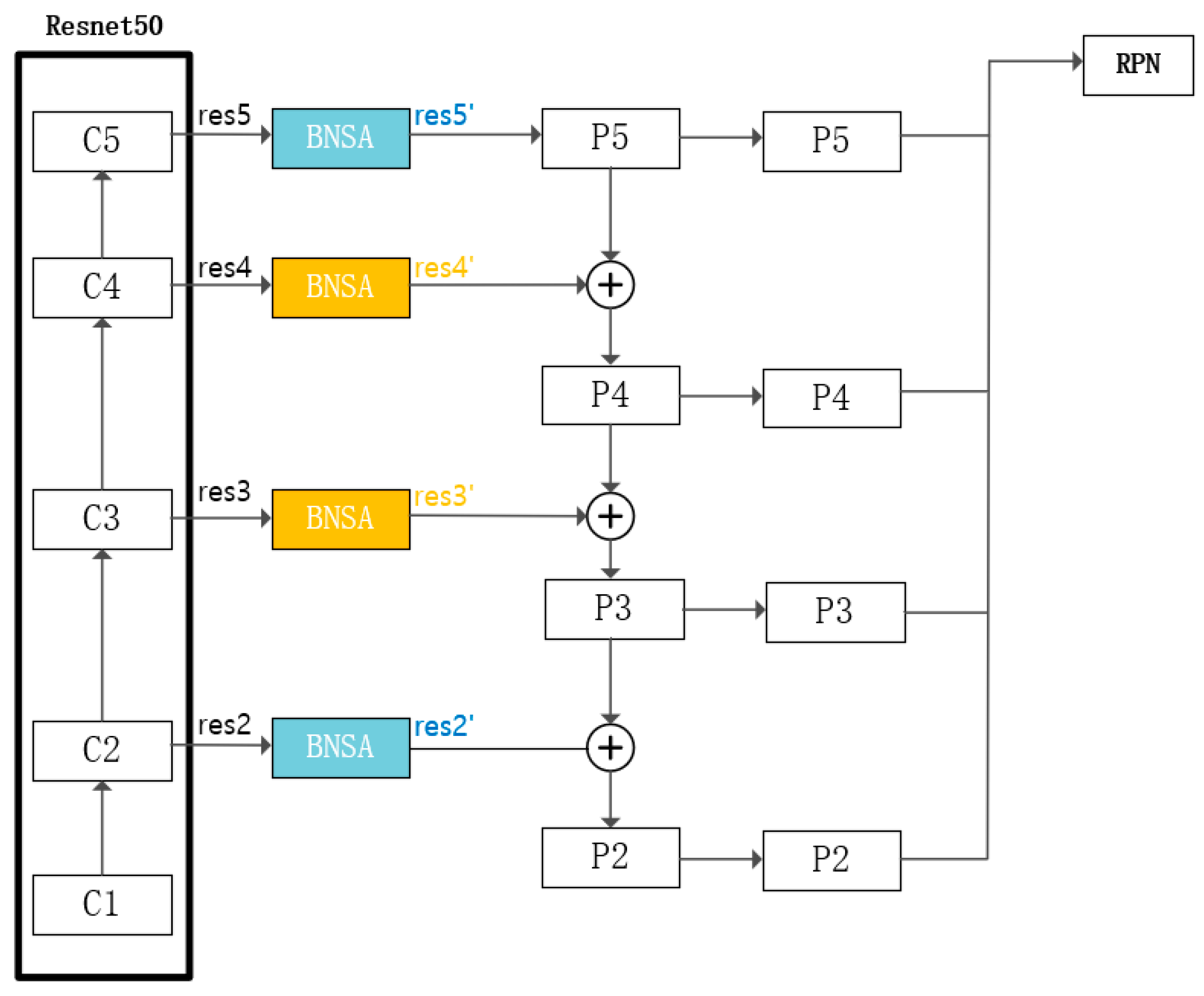
By incorporating global contextual information and capturing local details effectively, the BNSA module improves the overall performance of image feature extraction. Therefore, we integrated the BNSA module into the backbone network of Mask R-CNN. We inserted the BNSA module between ResNet and FPN layers, as shown in Figure 6, and conducted experiments to evaluate its performance. Based on the experimental results, we decided to insert the BNSA module after the output of C3 and C4 layers of ResNet. In Figure 6, these insertion modules are marked in yellow. The specific experimental procedure and results will be explained in Section 4.2.

The performance of the BNSA module was found to be highly sensitive to the specific insertion point within the backbone network. Through comparative experiments, it was observed that placing the BNSA module in either too shallow (e.g., C2) or too deep layers (e.g., C5) led to suboptimal results. The shallow layers primarily extract low-level features with limited semantic information, making it difficult for attention mechanisms to focus meaningfully. In contrast, the deepest layers contain highly abstract representations with reduced spatial resolution, which may cause the attention module to overfit or amplify noise, especially in low-texture infrared scenes. Inserting the BNSA module at intermediate levels such as C3 and C4 allows for a better balance between semantic richness and spatial detail, enabling more effective enhancement in target-relevant features. This experimental observation supports the design choice to integrate BNSA specifically at the C3 and C4 layers in our final architecture.

This design helps the network selectively enhance discriminative thermal features while suppressing redundant channel responses, which is particularly beneficial for infrared images where object boundaries are often blurred and texture details are limited.

3.3. Bounding Box Regression Loss Function Optimization

The Mask R-CNN network has a total of five types of losses, including classification loss (loss_rpn_cls) and bounding box regression loss (loss_rpn_loc) belonging to the RPN, as well as classification loss (loss_cls), bounding box regression loss (loss_box_reg), and mask loss (loss_mask) belonging to the prediction head. Among these, two classification losses use the cross-entropy loss function, while the two bounding box regression losses use the Smooth L1 loss function. The mask loss uses the mean binary cross-entropy loss function. In this section, we will explain the method of optimizing the bounding box regression loss function belonging to the prediction head.

The Smooth L1 loss function can be calculated using Equations (5) and (6):

$$L_{reg}(t_i,t_i^{\ast })=smoot{h}_{L1}(t_i-t_i^{\ast })$$

(5)

$$smoot{h}_{L1}(x)=\left\{\begin{array}{cc}0.5x^2& \left|x\right|<1\\ \left|x\right|-0.5& \left|x\right|\ge 1\end{array}\right.$$

(6)

In Equation (5), i represents the index of an individual ground truth box in each batch of images. $t_i$ is a vector representing the offset between the predicted bounding box and the anchor box; $t_i^{\ast }$ is a vector with the same dimensions as $t_i$, representing the offset between the anchor box and the ground truth bounding box.

However, in practice, the Smooth L1 loss function simply calculates the numerical difference between the predicted bounding box and the ground truth bounding box. As can be seen from Equation (6), when $\left|x\right|\ge 1$, the first derivative with respect to x is a constant. This constant derivative can have an impact on the descent of the loss value during late stages of training, potentially preventing the network from achieving better convergence results. To address this issue, we used a combination of SIoU Loss [33] and Focal Loss [34] for optimization.

The rationale for combining Focal Loss with SIoU stems from their complementary strengths in addressing different limitations of bounding box regression in infrared imagery. SIoU provides a direction-aware mechanism that penalizes misalignment between predicted and ground truth boxes, improving convergence in terms of geometric consistency. However, it lacks adaptiveness in weighting samples of varying quality during training. Infrared images often contain background clutter, weak object boundaries, and numerous false proposals, which can skew the learning process if all samples contribute equally. To alleviate this, Focal Loss is incorporated to dynamically down-weight poorly predicted boxes and emphasize high-quality samples by introducing an IoU-based scaling factor. This integration effectively suppresses the influence of noisy gradients from low-IoU boxes, stabilizes training, and accelerates convergence, especially in complex infrared scenarios with imbalanced sample distributions.

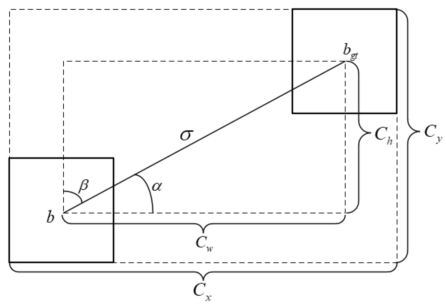
SIoU builds on CIoU [35] by considering the problem of direction mismatch between the predicted bounding box and the ground truth bounding box. It provides a direction for the predicted bounding box to approach the real box, thereby accelerating the convergence speed of the network model. Specifically, SIoU utilizes four penalty costs, including IoU cost, Angle cost, Distance cost, and Shape cost, to guide the correct descent of the loss value. Representing the Angle cost, $\mathsf{\Lambda }$ drives the predicted bounding box to move toward the horizontal/vertical distance closest to the ground truth bounding box. The formula is shown in Equation (7):

$$\mathsf{\Lambda }=1-2\times {\sin }^2(\arcsin (x)-{\displaystyle \frac{\pi }{4}})$$

(7)

$$x={\displaystyle \frac{C_h}{\sigma }}=\sin (\alpha )$$

(8)

where $\sigma =\sqrt{{(b_{c_x}^{gt}-b_{c_x})}^2+{(b_{c_y}^{gt}-b_{c_y})}^2}$, $C_h=\max (b_{c_y}^{gt},b_{c_y})-\min (b_{c_y}^{gt},b_{c_y})$, $(b_{c_x}^{gt},b_{c_y}^{gt})$ represents the center coordinates of the ground truth bounding box, $(b_{c_x},b_{c_y})$ represents the center coordinates of the predicted bounding box, and the remaining parameters used are given in Figure 7.

The calculation formula for the Distance cost $\Delta$ is shown in Equation (9). It calculates the distance between the center points of two bounding boxes and is greatly affected by the Angle cost. When the Angle cost decreases, the Distance cost also decreases correspondingly and vice versa. The Shape cost $\mathsf{\Omega }$ promotes the predicted bounding box to align its shape more closely to the ground truth box, as shown in Equation (10).

$$\Delta ={\displaystyle {\sum }_{t=x,y}(1-e^{-\gamma \rho t})}$$

(9)

$$\mathsf{\Omega }={\displaystyle {\sum }_{t=w,h}{(1-e^{-\omega t})}^{\theta }}$$

(10)

where ${\rho }_x={({\displaystyle \frac{b_{c_x}^{gt}-b_{c_x}}{C_x}})}^2$, ${\rho }_y={({\displaystyle \frac{b_{c_y}^{gt}-b_{c_y}}{C_y}})}^2$, $\gamma =2-\mathsf{\Lambda }$, $\theta =4$, ${\omega }_w={\displaystyle \frac{\left|w-w^{gt}\right|}{\max (w,w^{gt})}}$, ${\omega }_h={\displaystyle \frac{\left|h-h^{gt}\right|}{\max (h,h^{gt})}}$, $w$ and $w^{gt}$ represent the width of two bounding boxes, respectively, and $h$ and $h^{gt}$ represent the height of two bounding boxes, respectively.

Overall, SIoU Loss can be formulated as follows:

$$L_{SIoU}=1-IoU+{\displaystyle \frac{\Delta +\mathsf{\Omega }}{2}}$$

(11)

Focal Loss as described above is different from the Focal Loss used in classification losses. It aims to enhance the contribution of well-regressed predicted boxes to the overall regression loss. Due to the imbalance between foreground and background in an image, the predicted bounding boxes that closely match the ground truth bounding boxes account for a small proportion in the overall prediction results. However, high-precision regression predictions should have a larger impact on the gradients during the model training process [36]. And it is also necessary to suppress the weight proportion of the loss value for poorly regressed predicted bounding boxes. To achieve this, we combined Focal Loss with SIoU Loss to obtain the optimized bounding box loss function formula, expressed as Equation (12), where $\gamma$ is responsible for adjusting the degree of suppression of low-quality prediction boxes.

$$L_{Focal-SIoU}=Io{U}^{\gamma }{L}_{SIoU}$$

(12)

3.4. Mask Loss Function Optimization

In Mask R-CNN, the mask loss utilizes the mean binary cross-entropy (MBCE) loss. The mask prediction branch generates segmentation results based on the ROI results. For each ROI, it outputs k masks of size m × m, where k represents the total number of detected object categories in an image. m represents the size of the mask image, which is typically set to 28. Each mask prediction is associated with a specific object class. This means that each mask image contains the predicted segmentation mask for objects of the same class. To handle objects of category k, only the kth mask prediction is used to calculate the loss by comparing it with the corresponding ground truth mask. This approach avoids competition between different object categories effectively. It can be said that the mask branch in the Mask R-CNN network converts the multi-class loss calculation problem into multiple binary classification loss calculation problems. The specific formula is depicted in Equation (13):

$$L_{MBCE}={\displaystyle \frac{1}{m^2}}{\displaystyle \sum _j^k(1^k)}{\displaystyle \sum _i^{m^2}[-y_i\cdot \log (x_i)-(1-y_i)\cdot \log (1-x_i)]}$$

(13)

where i represents the index of pixels in the mask image. $x_i\in (0,1)$ is obtained by applying the sigmoid function to the output mask pixel values. $y_i\in \{0,1\}$ represents the positive or negative sample value of the current mask pixel. $1^k$ indicates that for objects belonging to category k, the loss is calculated only between the kth mask prediction and the corresponding ground truth. When the category is k, its value is set to 1, and when the category is not k, its value is set to 0.

MBCE Loss is essentially a per-pixel loss calculation function that primarily computes the loss based on local information within the image. However, when there is a severe imbalance between foreground and background or significant variations in the sizes of segmented objects in an image, MBCE Loss tends to learn the background or smaller objects, resulting in incorrect segmentation results. To address this issue, we incorporate Dice Loss [37] as a supplement to MBCE Loss. Dice Loss takes a global perspective and tends to focus on learning larger objects, independent of the foreground–background ratio. It complements MBCE Loss and is represented by Equation (14):

$$L_{Dice}={\displaystyle \sum _j^k(1^k)}(1-{\displaystyle \frac{2{\displaystyle \sum _i^{m^2}{x}_i{y}_i}}{{\displaystyle \sum _i^{m^2}{x}_i}+{\displaystyle \sum _i^{m^2}{y}_i}}})$$

(14)

In addition to MBCE Loss and Dice Loss, which both focus on learning the correct classification of mask segmentation results, we also incorporate the Lovasz–Softmax loss function [38] to complement the learning of differential features in cases of incorrect classification. The Lovasz–Softmax loss function utilizes the concept of Lovasz extension, where the generated predicted probability distribution results are expanded into ordered subsets belonging to different classes for loss computation. The following will explain this in detail.

We define $c\in {\mathbb{R}}^{m\times m}$ as the predicted label and $y\in {\mathbb{R}}^{m\times m}$ as the true label. The IOU Loss between the predicted and true labels can be formulated as follows:

$$\Delta (c,y)=1-{\displaystyle \frac{\left|c\cap y\right|}{\left|c\cup y\right|}}$$

(15)

As an alternative to IoU Loss, Lovasz–Softmax loss in Mask R-CNN can be formulated as follows:

$$L_{LS}={\displaystyle \sum _j^k(1^k)}\overline{\Delta }f(x_i,y_i)={\displaystyle \sum _j^k(1^k)}{\displaystyle \sum _i^{m^2}f(x_i,y_i)\cdot G(x_i,y_i)}$$

(16)

where $f(x_i,y_i)$ is the error function of the prediction result defined by Equation (17); $c_i\in \{0,1\}$ denotes the predicted label of pixel i belonging to class k. $G(x_i,y_i)=\Delta (S_i,y)-\Delta (S_{i-1},y)$; $S_i$ is the ordered set of segmented pixels corresponding to $x_i$. $x_i$ is sorted in the order of $x_{(i=0)}\ge x_{(i=1)}\ge \cdots \ge x_{(i=i)}\ge \cdots \ge x_{(i=m^2)}$, then $S_i$ sorts the $c_i$ corresponding to $x_i$ according to the sorting result, and $S_i=\left\{c_{(i=0)},c_{(i=1)},\cdots ,c_{(i=i)}\right\}$.

$$f(x_i,y_i)=\left\{\begin{array}{cc}1-x_i,\hfill & if{ \mathrm{c}}_i=y_i\hfill \\ x_i,\hfill & otherwise \hfill \end{array}\right.$$

(17)

In conclusion, the optimized loss_mask function is known as MBCE_Dice_LS Loss, and is formulated as shown in Equation (18). It is worth noting that we multiplied $L_{ls}$ by a coefficient of 0.1 to maintain consistency among the three loss values in terms of magnitude.

$$L_{MBCE\_Dice\_LS}=L_{MBCE}+L_{Dice}+0.1L_{LS}$$

(18)

4. Experiment Results

4.1. Experimental Configuration and Evaluation Indicators

All experiments in this section were conducted in a software environment consisting of Python 3.8 and PyTorch 1.10. Additionally, GPU acceleration was performed using NVIDIA GeForce RTX 3090 Ti (ASUS, Suzhou, China) (arch = 8.6) during the experiments. The dataset that was used in our experiments, as mentioned in Section 2, consists of a total of 2760 images. And the dataset was divided into training and testing sets at an 8:2 ratio with 2208 training images and 552 testing images. During the training process of our model, a learning rate of 0.001 was set, and the warmup method was applied to adjust the initial learning rate. The model was trained for a total of 100 epochs, and after the training, it was tested to evaluate its performance.

In the experiments, we primarily adopted evaluation metrics commonly used in the COCO dataset, namely mAP and Recall. These metrics were employed to assess the performance of the algorithm models. For the network model, four parameters can be obtained for object detection results: TP: true positive samples; TN: the number of true negative samples; FP: the number of false positive samples; FN: the number of false negative samples. These parameters can be used to calculate the Recall and Precision values, as shown in Equations (19) and (20):

$$\mathrm{Recall}={\displaystyle \frac{\mathrm{TP}}{\mathrm{TP}+\mathrm{FN}}}$$

(19)

$$\mathrm{Precision}={\displaystyle \frac{\mathrm{TP}}{\mathrm{TP}+\mathrm{FP}}}$$

(20)

Recall measures the proportion of correctly predicted samples among all samples, while Precision measures the proportion of correctly predicted results among all predicted results. AP is obtained by calculating the area under the Precision–Recall curve, where Recall values are plotted on the horizontal axis and Precision values on the vertical axis. And mAP is the average of AP values across different classes. It represents the overall performance of the model. A higher mAP value indicates better accuracy of the model. Additionally, mAP50 and mAP75 represent the mAP values when the IoU threshold exceeds 0.5 and 0.75, respectively. APs, APm, and APl refer to the mAP of target areas in different size ranges, with cutoff thresholds of 32 × 32 and 96 × 96.

4.2. Experiments and Ablation Analysis of the BNSA Attention Module

To evaluate the effectiveness of the proposed BNSA module, we conducted an ablation study by inserting the module at different levels (C2–C5) of the ResNet backbone, as illustrated in Figure 6. To qualitatively analyze its impact on feature representation, feature maps from each ResNet layer were visualized using a representative image from our dataset. For consistency, all feature maps were resized to the same resolution, and channels with significant responses were selected for display, as shown in Figure 8.

In Figure 8, the upper row shows the original feature maps before BNSA insertion, while the lower row shows the corresponding outputs after the BNSA module was added. Notably, the feature maps at layers C3 and C4 exhibit enhanced contrast and more defined semantic boundaries after applying BNSA, suggesting that attention has effectively improved mid-level feature localization. In contrast, applying BNSA at layer C2 leads to dispersed activation across irrelevant background regions, likely due to the large spatial size and low-level nature of early features. Similarly, at layer C5, excessive abstraction and smaller spatial resolution result in a loss of fine-grained detail, and the added attention module introduces redundant noise that slightly degrades the output quality.

These visual observations are corroborated by the quantitative results in

Table 1. An experimental comparison of the BNSA module inserted at different layers. The first column from top to bottom represents the results of inserting the BNSA module at the C2, C3, C4, and C5 layers and at both C3 and C4 layers simultaneously. Each row of the table presents the model metrics corresponding to each method. The results reveal that, except for mAP@50, which achieves the highest performance when the BNSA module is inserted at the C3 layer alone, all other metrics exhibit optimal results when the BNSA module is inserted at both layers, C3 and C4.

Method	mAP	Recall	mAP@50	mAP@75	mAPs	mAPm	mAPl
Without BNSA	63.400	0.684	95.820	73.164	55.832	74.703	75.565
C2 layer + BNSA	64.397	0.691	96.527	75.256	57.414	75.142	75.173
C3 layer + BNSA	64.922	0.696	96.728	78.051	57.454	75.075	75.102
C4 layer + BNSA	64.662	0.694	96.311	76.990	57.961	75.450	75.167
C5 layer + BNSA	63.955	0.689	96.012	74.902	56.474	75.315	77.419
C3 and C4 layers + BNSA	65.583	0.698	96.006	78.589	58.070	75.951	77.997

, where inserting BNSA in C3 and C4 simultaneously yields the best performance across most metrics. For comparison, we also evaluated the performance of the original Mask R-CNN model without the BNSA module. As shown in Table 1, the baseline results are consistently lower across all metrics, especially in mAP@75 and mAPs, confirming the effectiveness of the attention mechanism in improving both precise localization and small-object segmentation. This indicates that mid-level semantic features benefit the most from the BNSA module, striking a balance between spatial detail and semantic abstraction. Therefore, inserting the BNSA module at the C3 and C4 layers was adopted in the final model configuration.

4.3. Experiments of Bounding Box Regression Loss

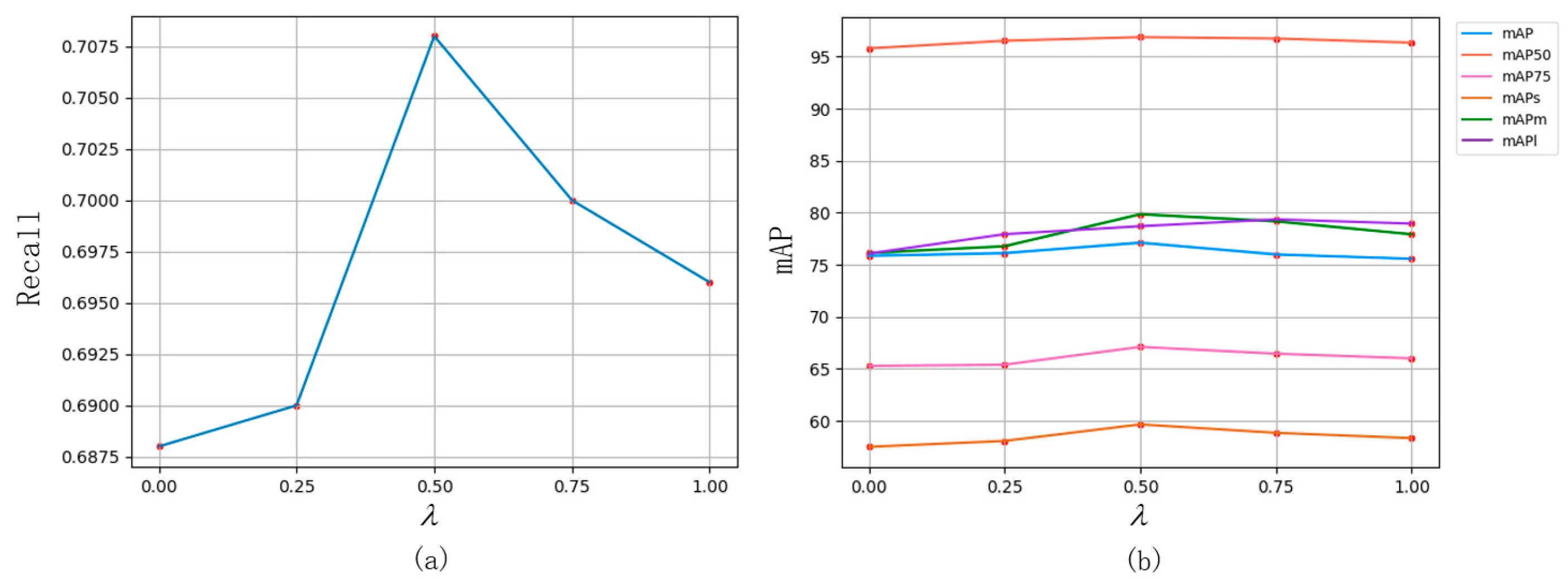
To obtain the best effect for the model with Focal_SIoU Loss, we experimented with different values of $\lambda$ and evaluated their impact on model accuracy. As shown in Figure 9, considering various metrics, it can be observed that overall model accuracy reaches its optimum when $\lambda$ is set to 0.5.

After determining the value of $\lambda$, we conducted experiments to compare the model accuracy of Mask R-CNN using its own Smooth L1 loss function with other IoU-based loss functions. We also tested the combination of various IoU-based loss functions with Focal Loss. The value of $\lambda$ was set to 0.5, as referenced in Figure 9. The experimental results are presented in

Table 2. A comparison of the experimental results with different bounding box regression loss functions. The first column, from top to bottom, represents seven different methods: Smooth L1, CIoU, EIoU [34], SIoU, Focal_CIoU (a combination of CIoU and Focal Loss), Focal_EIoU (a combination of EIoU and Focal Loss), and Focal_SIoU (a combination of SIoU and Focal Loss). Each row of the table presents the model metrics corresponding to each method. The results indicate that Focal_SIoU Loss performs optimally across all values, except for being slightly inferior to CIoU Loss in the segmentation of large targets.

Method	mAP	Recall	mAP@50	mAP@75	mAPs	mAPm	mAPl
Smooth L1 Loss	64.602	0.693	96.359	76.504	56.818	75.582	77.225
CIoU Loss	65.089	0.687	96.289	76.998	57.774	74.638	79.263
EIoU Loss	66.188	0.696	96.321	78.979	58.952	75.621	78.352
SIoU Loss	65.287	0.688	95.785	76.133	57.514	75.865	76.079
Focal_CIoU Loss	66.344	0.699	96.534	79.071	58.926	76.001	78.891
Focal_EIoU Loss	64.695	0.684	95.779	74.812	57.105	74.177	72.501
Focal_SIoU Loss	67.115	0.708	96.865	79.852	59.671	77.120	78.705

, demonstrating that Focal_SIoU Loss performed best in all indicators, except for a slight inferior segmentation of large objects when compared to CIoU Loss.

This performance gain can be interpreted from both geometric and optimization perspectives. SIoU improves upon IoU-based losses by incorporating directional alignment and distance penalties, which enhance the spatial consistency between the predicted and ground truth bounding boxes. However, SIoU alone treats all regression samples equally, making it susceptible to noisy or low-quality proposals—common in infrared scenes with blurred edges or occlusion. The introduction of the Focal weighting term addresses this limitation by emphasizing well-predicted boxes and down-weighting uncertain ones based on their IoU quality. This selective focus accelerates convergence and improves regression robustness, especially for small or low-contrast infrared targets. The results validate that the combination of SIoU’s geometric awareness and Focal Loss’s sample re-weighting contributes to more accurate and stable bounding box localization.

4.4. Experiments of Mask Loss Function

We tested the mask loss optimization method mentioned in Section 3.4, based on MBCE Loss. Firstly, we combined Dice Loss with MBCE Loss. From the results in

Table 3. A comparison of the experimental results using different mask loss functions. The first column of the table, from top to bottom, represents three methods: using MBCE Loss alone, the combination of MBCE Loss and Dice Loss, and the combination of MBCE Loss, Dice Loss, and Lovasz–Softmax loss, respectively. Each row of the table presents the model metrics corresponding to each method. The results indicate that under the condition of using the combination of MBCE Loss, Dice Loss, and Lovasz–Softmax loss, the model achieves optimal performance across all metrics.

Method	mAP	Recall	mAP@50	mAP@75	mAPs	mAPm	mAPl
MBCE Loss	64.602	0.693	96.359	76.504	56.818	75.582	77.225
MBCE Loss+Dice Loss	65.292	0.700	96.312	78.207	58.141	76.182	79.265
MBCE Loss+Dice Loss +Lovasz–Softmax loss	66.480	0.708	96.548	79.679	59.189	76.935	80.878

, it can be observed that the model achieved significantly improved accuracy in recognizing large targets with this combination. Then, we further optimized the model by adding Lovasz–Softmax loss, which learns the difference features of misclassified examples. The experimental results show that the model achieved optimal performance in various metrics by using the three loss functions simultaneously.

The effectiveness of the MBCE_Dice_LS loss function stems from the complementary strengths of its components. MBCE enhances per-pixel classification accuracy, which is essential for delineating fine mask details. Dice Loss mitigates the foreground–background imbalance common in infrared datasets by rewarding region-level overlap rather than pixel-wise agreement. Lovasz–Softmax directly optimizes the IoU score, aligning the training objective with the evaluation metric. Their combination allows the model to jointly learn local accuracy, shape integrity, and metric consistency. In infrared images where object contours are often unclear and boundaries may be diffuse, this compound loss helps maintain mask completeness while suppressing misclassification at object edges. The ablation results confirm that no single loss function alone achieves the same balance between detail preservation and segmentation reliability.

4.5. Comparison with Other Models

We proposed adding the BNSA module into the Mask-RCNN framework. Additionally, we used Focal_SIoU Loss as the bounding box regression loss function and MBCE_Dice_LS Loss as the mask loss function. To validate the effectiveness of our proposed method, we compared it not only with Mask R-CNN but also with mainstream segmentation network models such as BlendMask, CondInst, BoxInst, Solov2, and SparseInst. The results are shown in

Table 4. A performance comparison of different models. The first column lists te seven different methods used, namely Mask R-CNN, BlendMask, CondInst, BoxInst, Solov2, SparseInst, and Ours. Each row of the table presents the model metrics corresponding to each method. The results indicate that our method achieves the highest metrics across all categories, except for the segmentation of large targets where the accuracy is lower than that of Solov2.

Method	mAP	Recall	mAP@50	mAP@75	mAPs	mAPm	mAPl	params
Mask R-CNN	64.602	0.693	96.359	76.504	56.818	75.582	77.225	44.343 M
BlendMask	65.350	0.701	96.189	77.781	56.881	76.867	80.988	35.982 M
CondInst	57.389	0.624	96.042	58.268	48.629	72.254	77.091	34.564 M
BoxInst	27.978	0.371	68.117	19.437	24.344	37.661	41.480	34.260 M
Solov2	57.489	0.612	88.798	61.682	44.404	74.971	84.671	46.540 M
SparseInst	46.400	0.518	88.100	41.000	36.900	58.200	66.900	31.618 M
Ours	68.460	0.718	97.229	82.278	61.798	77.394	80.007	53.865 M

. To assess stability, we repeated key experiments three times with different random seeds. The observed standard deviation of the mAP values was below 0.3, indicating stable and consistent performance. In addition, we also conducted a statistical analysis of the complexity of each model, represented by the trainable parameters ‘params’ of the model. The larger the value of ‘params’, the higher the complexity of the model. From the results in Table 4, it can be observed that although our method has a large number of model parameters, all other metrics are the highest, except for the segmentation accuracy of large objects. Compared to the original Mask R-CNN module, our method improves mAP by 3.858%, Recall by 0.025, mAP@50 by 0.87%, and mAP@75 by 5.774%.

In addition to our self-constructed dataset, we evaluated our method on the FLIR thermal dataset to assess generalizability. As shown in

Table 5. Performance on FLIR dataset.

Method	mAP	Recall	mAP@50	mAP@75	mAPs	mAPm	mAPl
Mask R-CNN	63.135	0.720	91.283	56.847	44.382	60.372	68.948
Ours	65.672	0.741	92.259	60.278	48.283	63.843	70.378

, our approach outperforms the baseline Mask R-CNN network across all metrics, especially in mAP@75 and small-object segmentation (mAPs), indicating good transferability across thermal imaging domains.

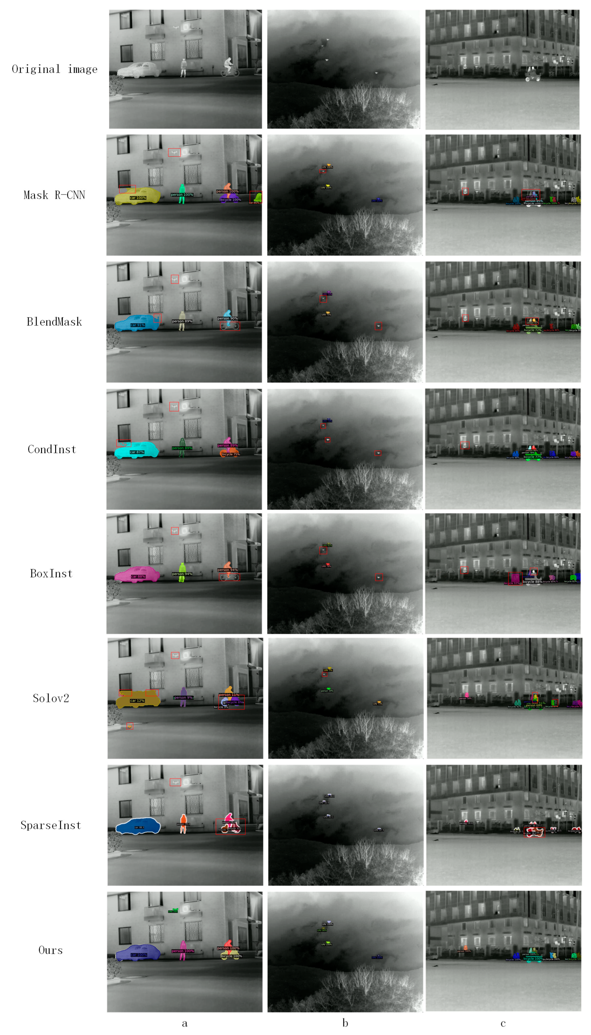
More intuitive segmentation results are displayed in Figure 10. We have selected three images from the dataset as examples. The red boxes indicate the parts of the results that were missed or misidentified. From Figure 10a, it can be observed that our proposed method detected all targets in the image and achieved more accurate overall segmentation results, without producing scattered color blocks as observed in other models. In Figure 10b, our method demonstrated its superiority in the segmentation of small targets. Even for drone objects with very small areas, our method can identify and segment them with high confidence. In Figure 10c, only the CondInst model and our method segmented multiple nearby targets correctly and completely. Moreover, our method exhibits higher confidence in the detection results compared to CondInst, ensuring the accuracy of segmentation.

In summary, our proposed method has certain advantages over other models in terms of detection accuracy, classification, and segmentation performance for infrared object detection. Compared to other mainstream instance segmentation models, the proposed method shows clear advantages in infrared scenarios characterized by background clutter, multi-class interference, and low target visibility. For example, CondInst and Solov2 rely heavily on mask head prediction without sufficient spatial refinement, often resulting in coarse or fragmented masks. BoxInst, while efficient in weakly supervised settings, lacks fine localization capability due to its limited reliance on pixel-level guidance. In contrast, our model benefits from the mid-level attention enhancement introduced by the BNSA module, which strengthens feature concentration around targets. Moreover, the redesigned loss functions contribute to stable training and precise mask boundary extraction. As visualized in Figure 10, our method generates more complete and accurate masks, especially for small objects such as UAVs and bicycles. This demonstrates the effectiveness of the proposed approach in addressing the inherent challenges of infrared image segmentation.

While the introduction of the BNSA attention modules leads to a slight increase in the number of trainable parameters, their computational cost remains relatively low due to the lightweight bottleneck structure. Moreover, since the modules are only inserted at selected mid-level layers (C3 and C4), the impact on overall inference speed is minimal. In practice, we observed that the increase in inference time per image was within an acceptable range, while yielding notable gains in segmentation accuracy—particularly for small and difficult infrared targets. Therefore, the performance–efficiency trade-off remains favorable.

5. Conclusions

In this paper, we utilized Mask R-CNN as the underlying framework for infrared image segmentation. We also added the BNSA module to the backbone network and optimized the bounding box regression loss and mask loss. The BNSA module incorporates global information from infrared images through the attention channel for feature learning. It enhances the segmentation accuracy of the model while introducing fewer parameters. The bounding box regression loss function, named ‘Focal_SIoU Loss’, comprises two aspects. One of them is the direction-guided nature of SIOU, and the other is the adjustment of the weight of the anchor boxes using Focal Loss. This approach accelerates the convergence speed of the network model. Further, the mask loss function of MBCE_Dice_LS Loss enhances model performance by considering global, local, and misclassification aspects without increasing model parameters. In addition, we created a new infrared image dataset to validate our proposed method. The experimental results demonstrate that our approach outperforms several mainstream segmentation networks in both accuracy and segmentation performance for infrared target recognition. In addition to improvements on our custom dataset, the model also shows consistent performance gains on the public FLIR thermal dataset, demonstrating its potential for broader infrared applications. Nonetheless, the proposed method still faces challenges, including relatively high model complexity and limited deployment flexibility. While the proposed method achieves strong results, there are still a few minor limitations worth noting. For example, although the BNSA module is lightweight and efficiently designed, it still introduces a slight increase in parameter count compared to the baseline. Additionally, the current framework does not explicitly consider temporal coherence, which may be relevant for certain video-based infrared applications. These aspects can be explored in future work to further enhance applicability.

In future work, we aim to make the model more suitable for deployment in practical infrared perception scenarios, such as UAV-based thermal monitoring, night-time surveillance, and industrial equipment inspection. In these applications, fast and accurate segmentation of low-contrast targets is critical. Therefore, future research will focus on compressing the network structure, reducing computational overhead, and enabling real-time inference on embedded platforms or edge devices with limited resources. In addition, we plan to explore domain adaptation techniques to improve the model’s robustness across varying thermal conditions and scene domains.