1. Introduction
In recent years, Deep Neural Networks (DNNs) have achieved unprecedented accuracy and results across a wide array of tasks [
1] ranging from image and speech recognition to natural language processing and autonomous control. However, training such models demands massive datasets, extensive computational resources, and deep expertise in architecture design and hyperparameter tuning. This investment of time, money, and human capital elevates high-performance NNs to the status of valuable Intellectual Property (IP) [
2], the protection of which is essential in both commercial and research contexts.
Prior to 2018, DNN inference was performed only on powerful cloud servers; however, this cloud-centric paradigm struggled to scale as the number of connected devices grew, raising concerns around connectivity availability, reliability, latency, privacy, and asset costs. To address these challenges, the TinyML (Tiny Machine Learning) community has emerged since 2018 [
3], enabling the deployment of “tiny” neural networks on microcontrollers (MCUs) and other resource-constrained low power edge devices. By compressing model architectures and quantizing their parameters (often to integers of 8 bits or even lower), TinyML approaches have enabled on-device intelligence with power budgets under a few milliwatts, fueling use cases from always-on keyword spotting to real-time anomaly detection in sensor networks [
4].
To provide an example, tiny NNs usually run on off-the-shelf MCUs that process information at several hundred MHz (the operative frequency of the MCU core), embedding up to 1 Mbyte of RAM and 2 Mbytes of FLASH on chip. The MCU can run tiny NNs that process data at either floating-point precision (fp32) or integer (e.g., 8 bits) with a range of performance adequate for most embedded edge AI applications currently available on the market.
While tiny networks have lower inference costs, they also exacerbate IP risks, since a small-footprint standalone binary embodying a trained model can be easily extracted, copied, or reverse-engineered [
5]. The Neural Network Watermarking (NNW) methodology has been proposed as a deterrent against unauthorized reuse and as a means to establish legal ownership. Inspired by classical multimedia watermarking in which hidden low-amplitude signals are embedded in images, audio, or video [
6], NNW seeks to embed a covert signature into the host model without degrading its performance.
Large NNs are inherently over-parameterized objects that can potentially perform well even after being subjected to simple transformations such as parameter quantization, pruning and fine-tuning aimed at overwriting the watermark. The effects of over-parameterization on the ability to make the DNN forget about specific information learned during training (e.g., the watermark) while maintaining high performances on the test set have been extensively studied in [
7]. NNs can also be easily duplicated. For these reasons, protection against tampering and integrity is not enough; it is also of paramount importance to guarantee that the watermark is robust against a wide range of transformations. Although numerous watermarking algorithms have been developed for large-scale DNNs, their applicability to tiny NNs is not straightforward. Tiny topologies feature far fewer parameters and operate under tight latency and memory constraints, leaving less “room” for watermark payloads and making them potentially more vulnerable to removal attacks. The ultimate goal of this work is to evaluate the viability of fine-tuning and post-training DNN watermarks in maintaining the extremely complex and precise task of training a DNN while embedding the watermark in the network as separately as possible.
The key contribution of this paper is to bridge the gap between NNW research and TinyML applications by adapting and evaluating three state-of-the-art watermarking techniques for resource-limited NNs. This work focuses on evaluating the efficacy of the implemented NNW methods on two image processing use cases: Image Classification (IC) by using the CIFAR-10 dataset [
8], and Visual Wake Words detection (VWW) using the COCO dataset [
9]. Specifically, this paper investigates the following:
Parameter-based embedding: A compact bit-string is injected into selected weight subsets during training (DeepSigns White-Box [
10]) or post-training (Tattooed [
11]).
Behavioral fingerprinting: Trigger inputs are designed that evoke unique activation patterns without compromising normal task performance (DeepSigns Black-Box [
10]).
Evaluation schemes: An attack pipeline is designed in order to attack both static and dynamic methods via common watermark overwriting attacks such as quantization, pruning, fine-tuning and Gaussian noise addition, allowing us to evaluate the strengths and weaknesses of different techniques when attacked using the most common DNN attack pipelines.
The experimental results demonstrate that all three approaches can reliably withstand realistic tampering while preserving the original accuracy, offering a practical toolkit for protecting TinyML models in real-world edge deployments.
2. Background on Watermarking
Watermarking refers to the process of embedding visible or imperceptible markers into host signals in order to assert ownership, verify authenticity, or trace distribution channels. Originating from physical watermarks in paper media, digital watermarking [
6] extends these concepts to multimedia data such as images, audio, video, etc., by covertly embedding meaningful information that survives even after common transformations are applied.
A Digital Watermark (DW) is a marker embedded within a carrier signal that can later be extracted or detected to prove ownership and/or integrity. A watermark usually does not increase the original file size and is designed to be robust against common processing techniques while remaining imperceptible to the end users unless specifically analyzed.
Digital watermarking schemes are categorized according to their resistance to modifications [
12]:
Fragile watermarks are destroyed by any modifications, and are used for tamper detection and proof of integrity.
Semi-fragile watermarks tolerate benign operations (e.g., compression of digital media) but detect malicious ones.
Robust watermarks survive a broad range of attacks, enabling copyright protection and source tracking.
Broadly speaking, watermarking schemes [
13] fall into two categories:
Static watermarking, in which a bit-string is encoded directly into weight values or network parameters during training.
Dynamic watermarking, where a special set of “trigger” inputs elicit an atypical yet deterministic response from the watermarked model, serving as a proof of ownership.
Both approaches must satisfy three key requirements:
Fidelity: The presence of the watermark should not degrade the original model’s accuracy.
Robustness: Watermark recovery should be guaranteed even after plausible tampering (e.g., fine-tuning or pruning, two of the most common ways of manipulating a DNN).
Capacity: The amount of information (i.e., number of watermark bits) that can be reliably embedded in the model.
The process of embedding a watermark inside an NN can be divided into two phases, namely, watermark embedding and watermark detection. The process begins by selecting a DW that will be embedded into the NN during the training or post-training phase. This can be achieved by subtly altering the parameters of the model, such as weights and biases, to inject the DW information; alternatively, it can be integrated into the inputs. After the DW has been embedded, the owner must be able to detect it in order to verify the authenticity of the model. This is typically performed using specialized extraction algorithms. These include trigger set-based detection [
14] carried out by analyzing model behavior on a set of specifically crafted inputs (the triggers), steganalysis-based detection [
15], and zero-bit watermarking [
16].
In the event that a malicious individual claims ownership of a copied proprietary IP, the watermarking method provides the true owner of the NN with an extraction method to detect and verify the presence of the watermark, allowing them to rightfully claim ownership of the model.
2.1. White-Box vs. Black-Box Watermarking
Based on the data accessible to the watermark extractor, DNN watermarking techniques can be divided into White-Box (WB) and Black-Box (BB) methods [
13]:
White-Box (
Figure 1a): The watermark is directly embedded among the model’s internal parameters and is extracted by directly accessing them. The internal parameters may correspond directly to the model weights or to the activations of the neurons in correspondence to specific inputs.
Black-Box (
Figure 1b): In this case, the watermark is also embedded in the model’s parameters, but only the final output of the DNN is accessible; extraction of the watermark is carried out by querying the model and checking the output of the DNN in correspondence to a specific set of inputs (trigger inputs).
2.2. Static vs. Dynamic Watermarking
An important distinction in watermarking techniques can be made between static and dynamic watermarking [
13].
Static (
Figure 2a): The watermark is statically embedded into the weights of the model; these weights are determined during training or post-training, and do not depend on the inputs provided to the NN.
Dynamic (
Figure 2b): The watermark is detected based on the behavior that the model exhibits in correspondence with specific inputs (triggers/keys); the watermark is still embedded by modifying the weights of the NN during training, but is retrieved by looking at the behavior of the model.
2.3. Embedding Modalities
Based on the moment in which the WM message is embedded within the DNN with respect to the training of the network on the main task, watermarking methods can be classified as training, fine-tuning, or post-training watermarking [
17]. The first attempts in DNN watermarking were carried out by embedding the watermark alongside training of the DNN on the main task in order to ensure optimal performance preservation during the embedding phase. However, when working with DNNs, embedding during training not always a viable possibility. Because training a large network can be an extremely expensive and time consuming practice, a great deal of research has also focused on the possibility of watermarking an already trained DNN by fine-tuning [
18], making the embedding process much faster and more convenient (
Figure 3a). In addition to these two already consolidated DNN watermarking strategies, post-training watermarking is also beginning to garner attention as an effective and very low-cost watermarking modality. The work proposed in [
11] represents one of the firsts post-training watermarking methods (
Figure 3b). This approach has proven to be robust to a wide array of attacks, making it an important step toward the future of DNN watermarking.
3. Related Works
In the past, only a limited number of certified institutions could serve as outlets for the distribution and monetization of IPs. This dynamic has shifted dramatically with the advent of digital media and technological advancements, which make it exceedingly easy to copy, modify, and redistribute digital objects, often with the intent to resell stolen IPs. In this chaotic landscape, digital watermarking emerges as a crucial solution to protect IPs from piracy [
19].
Digital watermarking is vital because it offers a secure and reliable method for copyright protection, content tracking, and rights management, ensuring that creators and rights holders maintain control over their digital assets even as they are shared and distributed online. The first significant approach to digital watermarking was introduced in 1994 by Tirkel et al. [
20] utilizing steganography. Steganography involves concealing information within another message or physical object such that the hidden information’s presence is not evident to an unsuspecting observer. Embedding a message inside a digital object in a manner detectable only under specific conditions, such as applying a particular algorithm or function, is central to many recent digital watermarking techniques.
3.1. Digital Image Watermarking
Digital image watermarking can be divided into two main categories: spatial domain techniques and transform domain techniques. In the spatial domain, the watermark is inserted directly into the pixel values, modifying only the least significant bits through methods such as LSB [
21] to covertly inject information without altering visual quality. Transform domain techniques involve transforming an image and embedding the watermark in the transformed image’s coefficients, which is achieved through methods such as the Discrete Cosine Transform (DCT) [
22], Discrete Wavelet Transform (DWT) [
23], Discrete Fourier Transform (DFT) [
24], or dimensionality reduction methods such as Singular Value Decomposition (SVD) [
25].
As discussed by Sri Vadana [
26], in addition to preserving visual quality in image and video watermarking, the ultimate goal is to develop watermarking methods that adhere to specific behavioral standards, including:
Robustness: The capability of the watermark to resist common transformation methods.
Security: Ensuring that the watermark cannot be read by a third party.
Fragility: The opposite of robustness; a fragile watermark is one that does not survive transformation (e.g., copying or forging).
Key Restrictions: The level of restrictions placed on the detection ability of the watermark.
False Positive Rate: The probability of falsely detecting a watermark in an unmarked object.
Multiple Watermarks: The ability to insert multiple watermarks into the same object.
Data Payload: The amount of information stored in the mark.
Computational Cost: The cost of injecting and detecting the mark.
While initially proposed for digital image watermarking, these properties remain valid for the evaluation of many other watermarking pipelines, including NNW, where they are used to study the behavior of models undergoing a range of attacks aimed at erasing watermarks.
3.2. Neural Network Watermarking
Similarly to digital images, where operations are applied on a matrix of pixel values, many layers in modern NNs posses at least one weight matrix (e.g dense, convolutional, or recurrent layers) [
27], making them optimal information carriers for watermarking purposes. It is exactly by leveraging the weight matrices that the first NNW pipelines emerged. Generally speaking, the NNW process can be divided into the following phases:
Message Encoding: In this phase, the message is transformed into an embeddable format.
Embedding: The encoded message is embedded in the model parameters.
Extraction: The watermark is extracted from the model using a specific algorithm.
Decoding: The extracted message can be decoded when necessary, usually by applying the inverse of the encoding transformation applied in the encoding step.
Verification: To confirm that the watermark is present in the model, the extracted message is compared to the original one evaluating the presence of the watermark in order to confirm model ownership.
As stated in
Section 2, watermarking pipelines can be divided into white-box and black-box methods based on the data accessed by the watermark extractor.
3.2.1. White-Box Watermarking
One of the first papers on WB NN watermarking was published by Uchida et al. [
28], who studied the possibility of embedding an
N-bit vector
in the parameters of one or more layers of a DNN by setting a custom regularizer in each target layer. The presence of the custom regularizer adds a regularization term to the original cost function, imposing a certain statistical bias during error-backpropagation that is inherited by the weights in the target model. A custom regularizer was also used in the creation of the first fingerprinting method for large-scale model distribution systems through model fine-tuning, as presented in [
14]. This approach embeds a
v-bit binary code vector
, where
is the index for each distributed user and
n is the total amount of users. As stated in
Section 2.2, watermarking information can also be embedded and extracted from dynamic components of the network, such as the activations of each layer, as presented in the white-box method of [
10]. There, the authors used a custom loss function to modify the probability distributions of the features computed by the target layers during a fine-tuning phase in order to embed the WM information.
3.2.2. Black-Box Watermarking
Unlike typical digital objects, NNs can be trained to exhibit specific behaviors when presented with abnormal inputs (e.g., trigger inputs) that would otherwise elicit completely different responses from an unmodified model. This unique property underlies many backdoor BB watermarking techniques adopted for DNN watermarking. One of the earliest efforts in this domain was presented by Zhang et al. [
29], who embedded meaningful content into original training samples to create trigger-based watermarks. A completely different approach was adopted in [
30], where the DNN was trained to produce watermarked images in response to designated triggers. This was achieved by incorporating a reconstructive regularization that instructed the model to map each trigger input to a predetermined output. Their work also emphasized the critical role of selecting an appropriate transformation function that produces a trigger set distribution maximally distinct from that of the original data, thereby enhancing watermark robustness and detectability. In
Table 1 are compared all the related White-box and Black-box NNW techniques explored in the work.
3.3. Attacks
As interest in DNN watermarking grows rapidly among researchers, numerous attack strategies have been developed to remove watermarks from DNNs while maintaining their performance. Consequently, ensuring the robustness of watermarks against such attacks has become a critical challenge in advancing DNN watermarking techniques. Among the various attack types, model modification and model extraction are considered the most effective methods for compromising the integrity of watermarks.
Table 2 summarizes common attack techniques designed to erase watermarks from DNNs.
4. Problem Statement
This manuscript addresses the challenge of applying white-box and black-box DNN watermarking techniques to tiny NNs while ensuring that the insertion of the watermark does not impact performance, inference time, or memory footprint (all critical constraints for the deployment of DNNs on resource-limited systems such as MCUs). Additionally, the methods explored in this work are chosen so as to avoid training the DNN from scratch.
Requirements for deployment on MCUs: The MCUs used in this paper consist of the popular off-the-shelf STM32, which has 1 MB of RAM and 2 MB of Flash memory integrated on chip along with an operational core frequency of up to 400 MHz. The DNNs must meet these constraints both before and after watermarking, focusing on maintaining low latency and preserving original performances.
Watermarking Modalities: This paper discusses methods for embedding watermarks without the need to retrain the model from scratch or modify the model topology utilizing fine-tuning or post-training techniques. For this reason, other well known state-of-the-art NNW techniques such as RIGA [
39] and Passport [
40] are not taken into consideration by this study. In this context, special attention is placed on choosing the appropriate data subset size and number of epochs required for the WM process in order to ensure a reasonable tradeoff between the amount of WM information embedded in the model and its impact on model accuracy.
Properties of the Watermark [
41]: The watermark should be
imperceptible, meaning that the difference between marked and unmarked models is undetectable to third parties. In addition, the model must have sufficient
Capacity, referring to the amount of watermark information that can be embedded while maintaining performance, while also ensuring
Uniqueness and
Secrecy. These latter two properties are vital for this work, as each watermarking process uses a unique secret key to generate the embedded message.
Robustness and Security: In order to be applicable to real world settings, a watermark must be robust against a wide range of model modification and model extraction attacks, allowing ownership verification for models suspected of being stolen or tampered with by malicious entities and ensuring effective IP protection. This paper presents the results after four of the most common modification attacks, namely, fine-tuning, pruning, Gaussian noise addition, and quantization; these results can be found in
Section 9.
5. Use Cases
MLCommons [
42] is an AI engineering consortium founded on the principle of open collaboration to enhance AI systems. By combining efforts from industry and academia, it aims to measure and improve the accuracy, safety, speed, and efficiency of AI technologies, aiding companies and universities in developing superior AI systems for societal benefit. Tiny MLPerf Inference, one of its working groups, has since 2020 established a benchmark suite that evaluates the speed and energy at which tiny edge device systems can process inputs and generate results using specific pretrained neural network models. The experimentation carried out in this work considers two of the four tiny MLPerf use cases: Image Classification (IC) and Visual Wake Words (VWW), which are explored in
Section 5.1 and
Section 5.2 respectively.
5.1. Image Classification
The CIFAR-10 dataset is used [
8] for the Image Classification (IC) task. This dataset consists of 60,000 32 × 32 × 3 color images divided into ten classes of 6000 images each; 50,000 images were used for training and validating the baseline models, while the remaining 10,000 were used for testing. The model used for IC is a custom resnet-8 [
43] provided by MLCommons, where the number of residual blocks was reduced from four to three. The model takes images with size 32 × 32 × 3 as inputs and produces a probability vector of size 10 as output. The pretrained model occupies 96 KiB after TensorFlow Lite (TFL) quantization, which is found on the vast majority of modern MCUs.
5.2. Visual Wake Words
The Visual Wake Words (VWW) dataset is used for the task of detecting the presence of a person in an image [
9]. It results from filtering of the COCO dataset [
44], and provides 115 k 96 × 96 × 3 images with “person” or “non-person” labels. Each image occupies only 27 KiB of storage, making it optimal for the development of models designed for visual tasks on MCUs. The network used for the VWW task is MobileNetV1 [
45], which takes inputs of size 96 × 96 and performs depth-wise convolutions that produce two-class outputs (i.e., person and no person). The TFL version of the pretrained model occupies only 325 KiB of memory, making it a valid option for human detection on edge devices.
6. Modeled Approaches
As discussed in
Section 2.3, the objective of this work is to explore and evaluate the applicability to tiny NNs of watermarking techniques that avoid training the NN from scratch. For this reason, our work investigates one fine-tuning-based WM technique for both WB and BB frameworks along with one post-training WB WM technique. These methods are explained in detail in
Section 6.1,
Section 6.2 and
Section 6.3 respectively. This paper also evaluates the effectiveness of these watermarking approaches and their effect on model performance. All the methods discussed in this paper have been tested for both IC (
Section 5.1) and VWW (
Section 5.2) use cases.
6.1. Fine-Tuning White-Box Method
Fine-tuning-based watermarking relies on carefully finding an optimal tradeoff between the resources used for the fine-tuning step (e.g., number of epochs, number of samples) and the robustness of the watermark to be embedded in the model through a limited number of training iterations. For this WM modality, the DeepSigns method [
10,
15] was chosen due to its box-agnostic approach, which makes it implementable for both WB and BB use cases. The WB implementation of DeepSigns is dynamic; the WM information is embedded in the features, computed from the activations of one or more target layers. The Probability Density Function (PDF) that characterizes the data distribution of the activations is assumed to be a Gaussian Mixture Model (GMM), a probabilistic model in which all the data points are generated from a mixture of a finite number of Gaussian distributions. By adding a regularization term to the total loss, as explained in
Section 6.1.1, the model is encouraged to generate activations that follow a Gaussian PDF with respect to each target class of the dataset. This ensures statistical symmetry and consequently robustness to extreme model perturbations, as described in
Section 9.
6.1.1. Embedding the Message
The process used to embed the watermark can be divided into the following two steps:
Key Generation: During this phase, all of the objects required for the watermarking procedure are generated. The user specifies the desired length N of the message to be embedded and the target classes s. These classes are then used to generate the activations of the target layers in which the watermark is going to be embedded, which coincide with the number of Gaussian distributions chosen to embed the WM. Next, one or more target layers l are selected. In the implementation presented in this paper, only one layer is chosen as the target, which is a layer in both ResNet8 and MobileNetV1.
The activations produced by the
l layers are used to compute the class means
(the mean values of the GMMs generated using the
s selected classes), where
M is the size of the feature space. A projection matrix
is also randomly generated to encrypt the class means into the binary space, as presented in the following equations:
Equation (
1) describes the generation of the matrix
that is obtained by applying a sigmoid function on the projected values. This procedure generates a matrix with values
with size
. As described in Equation (
2), this matrix is used to compute the extracted message
. The values of
are binarized using a threshold of
.
Model Fine-Tuning: To encode the WM in the model, only the activations generated by the target classes
s are used to compute the class means of the GMMs (following the Gaussian PDF assumption), and the distance between the original message
b and extracted message
is minimized during training. To ensure that both these requirements are met, two terms (
and
) are added to the original loss (
), among which
is a center-based contrastive loss [
46] that pushes the PDF distribution computed on the target classes into a Gaussian distribution in order to ensure the Gaussian distribution assumption, while
is a Binary Cross-Entropy (BCE) loss function [
47] that lets the model learn how to minimize the distance between
and
b, effectively embedding the watermark into the class means. The total loss is then computed as
where
and
are carefully selected hyperparameters. At the end of the fine-tuning process, DeepSigns inserts the WM information into the activation of layer
l and saves the original message
b, projection matrix
, and selected classes
s that will be needed later for WM extraction.
The watermarking process is shown in
Figure 4.
6.1.2. Extracting the Watermark
Watermark extraction follows the inverse procedure of the embedding process. A batch of 8192 samples taken from the original dataset is used as the input. The class means
of the GMMs are computed from the activations generated by the target layer
l on the selected classes
s. Then, following Equations (
1) and (
2) in this order, DeepSigns computes the extracted binary message
. To evaluate the presence of the watermark in the model, the Bit Error Rate (BER) is computed between
and the original message
b, calculating the percentage of mismatching bits between the two messages. Extraction of the watermark is carried out as shown in
Figure 5. A low BER value indicates that the original message
b and extracted message
are very similar, confirming that the watermark has been correctly embedded in the model activations.
6.2. Fine-Tuning Black-Box Method
The DeepSigns BB method is based on the idea of watermarking a DNN by backdooring it during a fine-tuning step. This approach, first explored by Adi et al. [
48], is carried out by mixing handcrafted inputs together with the original data.
6.2.1. Embedding the Watermark
The watermark embedding procedure follows three key steps:
Key Generation: A set of K unique input samples is generated, each of which is a tuple (data, label), where “data” refers to the pixel values of the trigger image and “label” is its crafted label. These form the trigger inputs used as watermarking keys. The first step of the WM process consists of passing the trigger inputs through the pretrained non-watermarked DNN, which outputs a set of K predictions. These predictions are then used to compute the mismatches scored by the unmarked model on the trigger set.
Fine-Tuning: During this step, the model is fine-tuned using a subset of the original dataset to which the trigger inputs generated in step 1 have been concatenated. During this phase, the model learns to predict the random labels assigned to the trigger data while also retaining its accuracy on the original dataset. By carefully selecting the number of samples taken from the original dataset with respect to the number of triggers used for WM, the model is overfitted on the triggers, effectively watermarking it while preserving its generalization capabilities on unseen data. This is verified by the results obtained in
Section 7.1 and
Section 7.2.
Key Selection: At the end of the fine-tuning process, the now-watermarked model is queried again on the trigger set, producing a new set of K predictions. Unlike the key generation step, only the correct predictions are used to select the key inputs that have been correctly classified. The set of mismatched key inputs (found in step 1) and those that have been classified correctly (found in step 3) are now intersected, meaning that only the trigger samples that were initially misclassified and that are now classified correctly after the fine-tuning step are selected, producing a set of valid keys . If the number of valid keys is at least equal to the desired length of the watermark, the process is terminated and the model can be considered successfully watermarked. Otherwise, the watermarked model is discarded and a new fine-tuning process begins by re-initializing the watermarking process from step 2.
The watermarking process is summarized in
Figure 6.
6.2.2. Extracting the Watermark
Watermark extraction and detection is carried out as shown in
Figure 7. First, the model is queried using the generated set of key inputs
, producing a set of predictions
; these are the output labels corresponding to the input keys. Second, the number of mismatches
between the ground truth labels
and predicted labels
is calculated. Finally, a decision threshold
is set; if
, then the presence of the WM is confirmed.
6.2.3. Trigger Datasets
A trigger dataset consists of a small specially-crafted collection of inputs paired with unique labels. These inputs have the same input format (e.g., dimensions, data types) expected by the DNN and are statistically unrelated to the standard training samples. Typically, the trigger set is composed of a small amount of samples, generally less than of the training data. A label is assigned to each trigger sample based on a secret mapping known only by the model’s owner; both the method used to generate these inputs and the labels mapping must remain confidential in order to ensure that only the owner can use them to identify the WM. During training, the trigger data are merged with the standard training samples; as a result, the NN learns to associate the trigger data with their assigned labels without losing accuracy on the original task. This procedure is also referred to as watermarking via backdooring. To prove the presence of the WM in the model and thereby demonstrate model ownership, the trigger data are fed to the model by consistently producing the secret labels, verifying the success of the WM procedure.
6.2.4. Trigger Set Composed of Random Symmetric Shapes and Colors
Each image is generated by first defining its two-dimensional coordinate grid, which serves as the drawing surface. A series of functions ranging from simple arithmetic and trigonometric operations to random color generators is then used recursively to build complex expressions. In this way, each pixel’s red, green, and blue values are computed using a unique mathematical formula. Following this procedure, a set of images containing a series of geometrically symmetric patterns and shapes (e.g., squares, circles, etc.) is generated. The presence of such patterns makes each trigger more distinct and easier to detect even at low resolutions. After computing this low-resolution prototype, the image is scaled up to the target size and its pixel intensities are quantized into standard 8-bit RGB values (0–255 range). Examples of images produced following this process can be seen in
Figure 8.
6.2.5. Trigger Set Composed of Preselected Images
Another approach consisted in using a preselected set of uncorrelated random images. This ensures that the trigger set is unique and not easily replicable, which are fundamental aspects for the security and confidentiality of the watermark. The images selected following this process (see
Figure 9) are then resized and processed for use as trigger samples.
6.2.6. Trigger Set Composed of GAN-Generated Images
Unique trigger samples can also be synthesized using a pretrained Generative Adversarial Network (GAN). The GAN is composed of two objects: the generator (G) and discriminator (D). During training, G and D take part in a two-player game in which G transforms random noise vectors into images while D learns to distinguish these fake images from real examples. By using feedback from D to refine G through alternating updates, the generator gradually learns to produce more convincing images. However, in the context of this paper the goal is not perfect realism but rather distinctiveness; each output needs to be classifiable while also being uncorrelated with the others. The generation process begins by first loading model G pretrained on the CIFAR-10 distribution, then feeding it random latent vectors consisting of compact numerical representations of the inputs in a lower-dimensional space and collecting its raw outputs. These images are initially at the GAN’s native resolution, with pixel values in the
interval due to the
activation. In the next step, they resized to meet the network’s input size requirements and remapped into standard RGB color space (0–255 range). Finally, the entire batch is saved as a NumPy array for ease of use. In the context of this work, the GAN is pretrained on the two datasets presented in
Section 5.1 and
Section 5.2 ensuring preservation of the latent symmetries (e.g., symmetric textures and patterns). This facilitates the training process, especially when working with low-resolution images. Examples of images generated following this procedure are shown in
Figure 10.
6.3. Post-Training White-Box Method
Post-training watermarking refers to the process of embedding a WM in an NN without the need to train or fine-tune the network. As an exmaple, insertion of the WM in the model can be carried out by carefully modifying its weight values. This is the method followed by TATTOOED [
11], the post-training WM method explored in this paper. The main challenge presented by this method is ensuring that the marked model is not subject to noticeable performance degradation while also embedding sufficient watermarking information to make the WM robust against a variety of model modification attacks aimed at overwriting it. To ensure robustness while keeping the memory footprint as low as possible, the CDMA and LDPC algorithms are selected to encode and decode the WM. Efficiency is achieved by leveraging symmetrical properties such as orthogonal low-correlation spreading codes for CDMA and regular repeating structures of the parity-check matrix for LDPC. The tradeoff margin between WM robustness and performance degradation becomes especially tight when working with tiny NNs, as the number of parameters that can carry WM information is limited. This causes degradation of rapid model performance with even small modifications to the model parameters.
6.3.1. Embedding the Watermark
Following the categorization presented in [
13], TATTOOED is a
white-box,
multi-bit, and
blind NN watermarking technique. It relies on the application of Code Division Multiple Access (CDMA), leveraging spread spectrum techniques to spread each bit of the
m-bit watermark using a different CDMA spreading code. In this way, TATTOOED is able to spread each bit of the message as if it were transmitted at the same time by a different user. The weights of the DNN chosen to house the watermarking information can be seen as noise in the communication channel. The use of CDMA makes the watermark hard to detect and robust to changes in the DNN’s weights.
During the WM embedding process, the watermark
m passes through a Low-Density Parity Check (LDPC) encoder. LDPC is a family of error correction codes that introduces redundancy in order to transform
m into a redundant message
with
P bits, which is then embedded into the model’s
W parameters. The use of LDPC is fundamental to ensuring that the watermark is robust against model modifications. A secret key known only by the user is used to produce a unique seed by passing it through a hashing function. The seed generated following this procedure is then used to set the RNG state of the entire process. The bits of the watermark are encoded as a vector of
values, and the code generated for each bit is represented by
, which is a vector of
values with length
R, where
R is the number of parameters of the model. Here,
C is the
matrix that collects all the codes; this matrix is a secret known only by the legitimate owner of the model, who also owns the secret key used to generate it. The procedure used to embed the watermark in the model parameters is presented by the following equation:
where
W represents the vector containing the model weights and
is a hyperparameter that affects the strength of the watermarking process. The procedure used to compute
is also shown in
Figure 11a.
6.3.2. Extracting the Watermark
The legitimate owner can recover the watermark by following the inverse of the WM procedure presented in
Section 6.3.1, as shown in
Figure 11b. With access to the weights of the Tattooed DNN
, the legitimate owner can retrieve each bit
i of the redundant message
as follows:
where
is the transpose of
. The message
reconstructed from each
bits passes through an LDPC decoder, retrieving the original message
m.
6.4. Experiment Settings
As stated in
Section 6.1,
Section 6.2 and
Section 6.3, the two DeepSigns methods are both carried out through model fine-tuning, while TATTOOED is a post-training method. Regarding method complexity, DeepSigns introduces a linear time complexity that is proportional to the number of epochs used in the fine-tuning step multiplied by the number of activations firing at each training step. TATTOOED also introduces a time complexity that is linearly proportional to the length of the WM message multiplied by the number of weights used to embed the WM. The settings used to conduct each experiment on the two use cases (IC and VWW) are summarized in the following sections.
6.4.1. DeepSigns White-Box
Image Classification: In the IC use case, two classes where chosen to carry the watermark information, with the second-to-last layer of the model chosen as target layer l. The model was fine-tuned to embed a 16-bit watermark using a batch of 8192 samples with two different learning rates: and . The lambda parameters were chosen as and , respectively.
Visual Wake Words: For the VWW case, which has only two possible classes, a single class was chosen to house the watermark; l was taken in the same way as in the IC case, and the watermark length was equal to 32 bits. The fine-tuning was carried out using a batch of 8192 values and with and . The chosen lambda values were equal to and , respectively.
6.4.2. DeepSigns Black-Box
Image Classification: The experiment was carried out by fine-tuning the model on 10,000 samples from the original dataset augmented with n generated trigger inputs using an and 10 epochs.
Visual Wake Words: The samples were taken in the same way as in the IC use case, and fine-tuning is carried out by using a for 5 epochs.
Two different WM lengths were used in the IC and VWW cases, respectively, allowing us to evaluate the impact on model accuracy and the robustness of the WM.
To update the learning rate, Stochastic Gradient Descent (SGD) was used in both the white-box (
Section 6.4.1) and black-box (
Section 6.4.2) settings, with
and
.
6.4.3. TATTOOED
Image Classification: A 32-bit WM was embedded using a ratio of parameters and with . The BER threshold used to define the success of the watermarking process was set as .
Visual Wake Words: In the VWW use case, the ability to use a significantly larger model (with almost three times the weight parameters of the model used for IC) makes it possible to embed a much larger WM. Thus, a 256-bit message was embedded using a ratio of and with . The threshold for the VWW case was set to .
7. Watermarking Results
This section reports the results achieved by both the non-watermarked and watermarked models on the original datasets using the three explored watermarking methods. The parameters used for each of the experiment configurations are those reported in
Section 6.4. It is also worth noting that the DeepSigns BB methods presented in
Table 3 and
Table 4 are those trained using the trigger datasets generated with the GAN following the process described in
Section 6.2.6.
7.1. Image Classification Results
The results shown in
Table 3 refers to the Image Classification (IC) task (see
Section 5.1). The findings indicate a decrease in accuracy on the original dataset compared to the baseline non-watermarked model, particularly for the two DeepSigns BB methods. This is attributed to the backdoor training approach used for these models, which makes them more susceptible to the effects of watermark embedding. DeepSigns WB and TATTOOED, although showing minimal main task accuracy drop, achieve worse WM detection results. This is expected, as both of these methods are white-box and the WM is computed by directly accessing the model parameters, making the extraction procedure more sensitive to the low number of the ResNet8 parameters.
When working with tiny NNs, the length of the watermarking message plays an important role in guaranteeing robustness and negligible model performance drop.
Figure 12 and
Figure 13 show how the main task accuracy and watermark accuracy of the DeepSigns models are affected by the insertion of WMs of different lengths inside the IC model.
Figure 12 shows the results obtained on models watermarked with DeepSigns BB; as expected, increasing the WM length and consequently increasing the number of trigger keys
causes the accuracy on the main task to drop progressively. Encouragingly, increasing the WM length from 16 to 256 bits induces only a minimal drop in main task accuracy (
) while leaving WM accuracy unaffected.
Figure 13 shows the results obtained using the DeepSigns WB pipeline. As explained in
Section 6.1.1, in the IC use case the watermark is embedded inside PDFs computed over two of the ten classes present in the dataset, meaning that the WM is a
matrix in which
and
N is the watermark length. As expected, increasing the length of the WM from 4 to 16 bits causes both the main task and WM accuracy to drop. Surprisingly, further increasing the number of bits causes the model to achieve considerably higher accuracy on the main task while leading to a substantial drop on WM accuracy. This behavior is caused by the limited amount of parameters in which to embed the WM; when the message is too long, the WM information cannot be meaningfully embedded in the features extracted from the target layer, and as the WM no longer acts as a valid constraint on the loss function, the model is now able to focus more on learning the main task.
7.2. Visual Wake Words Results
The results for the VWW task (see
Section 5.2) are shown in
Table 4. Similar to the IC case, a reduction in accuracy on the original dataset is observed. A key difference here is in the watermark accuracy achieved by the DeepSigns WB and TATTOOED methods. As white-box methods (see
Section 2.1), the watermark presence is determined from the model parameters. For this reason, the larger number of parameters in the MobileNetV1 network used for the VWW task compared to the ResNet8 network used for the IC task significantly benefits the watermark retrieval procedure.
7.3. Comparing the Results Obtained by Applying NNW on Large Models
This section compares the results obtained with tiny and large NN models when applying the same WM method from [
10,
11]. Both of these works embedded watermarks in large models with millions of parameters; in contrast, the ResNet8 and MobileNetV1 networks chosen for this study are composed of only tens or hundreds of thousands of parameters. For the BB and WB DeepSigns methods, the large network was WideResNet, with 36.5 million parameters [
10], while for TATTOOED the large network was VGG, composed of 132.8 million parameters [
11].
Table 5,
Table 6 and
Table 7 report the results for DeepSigns BB, DeepSigns WB and TATTOOED, respectively. The difference between pre-WM and post-WM accuracy was then computed to evaluate the effect of watermark insertion on the different models. As expected, the impact of watermarking on model accuracy is much smaller when embedded in larger models; nonetheless, the results obtained on the tiny NNs show that the accuracy loss induced by the watermark is not greater than
for the worst case. As in the previous experiments, ResNet8 was used for IC and MobileNetV1 was used for VWW.
8. Deployability
The deployability of baseline DNNs trained on the explored use cases (see
Section 5.1 and
Section 5.2) was evaluated based on the results achieved on ResNet8 and MobileNetV1 for the IC and VWW use cases, respectively. The MCU used to run the experiments was the NUCLEO-STM32H743ZI2, the specifications of which are shown in
Table 8.
Results of Deployment on MCU
Evaluation of the memory footprint and inference time of the DNNs was achieved through the ST Edge AI Developer Cloud (
https://stedgeai-dc.st.com/home, last access on 7 July 2025), a free online service that automatically deploys pretrained neural networks on ST MCUs by providing optimizations and achieving benchmarking on the real chip.
Table 9 shows the results measured after deploying the two DNNs on the NUCLEO-H743ZI2 board.
Because none of the watermarking methods presented in this paper require any modifications to the network topology, the original and watermarked models occupy the same amount of memory (Flash and RAM) and require the same inference time and energy for each inference. For these reasons and for the sake of brevity, only one model for each use case is listed in
Table 9.
9. Attack Results
To evaluate the robustness of the embedded watermarks, various model modification attacks were applied, with results shown in
Table 10 for the IC use case and
Table 11 for the VWW use case. The attacks included fine-tuning, weight quantization, weight pruning, and Gaussian noise addition, as listed in
Table 2. These attacks were applied to the models discussed in
Section 7.1 and
Section 7.2; refer to
Table 3 and
Table 4 for the baseline model performance before the attacks. Demonstrating watermark robustness against these attacks is crucial, as methods such as fine-tuning and quantization can be used without the intent to remove the watermark, especially in embedded environments where weight quantization and weight pruning are essential optimization techniques for reducing the amount of MCU assets required to run the DNN. The attacks were carried out using different strength values for each attack type:
Additive Gaussian Noise: Random values were sampled from a normal distribution , where S is the power of the attack and is the standard deviation. The sampled values were then summed to every weight parameter of the DNN.
L1 Pruning: For each model layer, the of the weight parameters with the smallest norm were set to 0.
Quantization: The model weights were quantized using a quantization interval of B bits.
Fine-tuning: The model was fine-tuned using and a number of epochs equal to E.
Each row in
Table 10 and
Table 11 corresponds to a particular type of attack with a specific strength. Each model was evaluated by measuring its accuracy on the original dataset and on the watermark before the attack (
acc_ref) and afterwards (
acc_atk). Different colors of the cells composing
Table 10 and
Table 11 are used to highlight the results with respect to specific thresholds computed on the original dataset and the watermark.
Original Dataset: Green color is used to highlight accuracy loss of the attacked model , yellow color to indicate results in which , and red color for all remaining results. These thresholds were set according to the experience acquired by deploying NNs on the edge devices; as observed in the field trials, accuracy drops of as much as can be tolerated.
Watermark: For the results achieved on the watermark, only two colors are used; results highlighted in green refer to correct detection of the WM after the attack, while those highlighted in red refer to cases in which the watermark could not be reliably recognized. The thresholds used for recognition of the trigger dataset or WM are shown in the two tables in the Computed Threshold row. To ensure reliability, this threshold value was algorithmically computed for each method based on factors such as the WM length, number of classes, and baseline accuracy. The accuracy achieved by the DeepSigns BB model on the watermark is referred to as the trigger dataset accuracy, while for DeepSigns WB and TATTOOED the accuracy on the watermark is computed as .
A watermarking method can be considered successful under the following conditions: (1) the accuracy on both the original and trigger datasets/watermark is valid (green or yellow for the original dataset, green for the trigger dataset/watermark); or (2) an attempt to remove the watermark (red in the trigger/watermark column) results in a significant drop in model accuracy on the original dataset (red in the original dataset column). The degradation trends of both main task accuracy and watermark accuracy after the attacks are visualized in
Figure 14 and
Figure 15 for the IC use case and in
Figure 16 and
Figure 17 for the VWW use case.
9.1. Attack Results for Image Classification Use Case
Following the reasoning provided in
Section 9, from
Table 10 it can be noted that each WM method applied to the models used for IC is robust against all tested attack types. The only way to successfully remove the watermark from the models is by using strong attack values that significantly degrade model performance, rendering the application housing the model unusable.
9.2. Attack Results for Visual Wake Words Use Case
Table 11 shows the results of attacks against the models used for the VWW task. As discussed in
Section 9, the success of the WM procedure is evaluated by considering both the accuracy of the attacked model on the original dataset and its performance on the watermark. Both DeepSigns black-box methods are particularly fragile to Gaussian noise attacks. With a strength value of
, it is possible to tamper with the original model by effectively removing the WM while maintaining acceptable accuracy on the main task, thereby compromising model ownership. Additionally, the 20-key version of the DeepSigns method is vulnerable to pruning attacks. With
, the WM can be successfully removed from the model. However, this is not the case for the 40-key version, where the watermark remains reliably recognized until the model becomes unusable. Other than these critical cases, all WM methods demonstrate robustness against the tested attack pipelines. This is especially true for the DeepSigns white-box and TATTOOED models, which exhibit a high degree of resilience against even the strongest attacks.
10. Conclusions
This work concerns about the applicability of fine-tuning and post-training neural network watermarking methods on tiny NNs. Three WM methods have been extensively evaluated to ensure that the watermark remains correctly identifiable and that the accuracy on the original data is not significantly affected by the WM process in order to verify the success of the watermarking procedures. We subjected watermarked DNNs to quantization, pruning, fine-tuning, and Gaussian noise attacks and extensively evaluated the results, proving the robustness of the watermarks against a series of malicious model modification attacks aimed at erasing them. While this paper has extensively studied the robustness of WMs to model modifications, other properties such as resistance to reverse engineering, imperceptibility, and probability of false positives have not been addressed and will be covered in future research. This work also verified the deployability of the presented DNNs by measuring the memory size, (RAM and FLASH) required by the networks and their respective inference times, for which we used the set of facilities provided by the ST Edge AI Developer Cloud service. For the black-box methods, three different alternatives for generating the trigger datasets were also tested. Considering the results achieved by the watermarked models before and after attacking them, the positive success of all tested watermarking procedures can be affirmed, validating their robustness against a wide array of attack pipelines as well as their applicability over tiny NNs developed for deployment on low-cost and low-power MCUs. Future research will thoroughly examine the ethical implications of embedding watermarks in tiny NNs, especially when deployed in sensitive or safety-critical applications. While watermarking is a valuable tool for IP protection, any alteration to the model, regardless of its scale, must be carefully evaluated for its potential effects on performance, reliability, and interpretability. Additionally, researchers should consider broader ethical concerns such as transparency, accountability, and the potential misuse of watermarking techniques in order to ensure that these practices align with societal and ethical standards.
Author Contributions
Conceptualization, R.A., A.C., M.L. and D.P.P.; methodology, R.A., A.C., M.L. and D.P.P.; software, R.A. and A.C.; validation, R.A. and A.C.; formal analysis, R.A., A.C., M.L. and D.P.P.; investigation R.A., A.C., M.L. and D.P.P.; resources, D.P.P.; data curation, R.A. and A.C.; writing—original draft preparation, R.A., A.C., M.L. and D.P.P.; writing—review and editing, R.A., A.C., M.L. and D.P.P.; visualization, R.A. and A.C.; supervision, M.L. and D.P.P.; project administration D.P.P.; funding acquisition, D.P.P. All authors have read and agreed to the published version of the manuscript.
Funding
This research received no funding.
Data Availability Statement
No new datasets were created by this work.
Conflicts of Interest
The authors declare no conflicts of interest.
Abbreviations
The following abbreviations are used in this manuscript:
| A | Adversary Network |
| AI | Artificial Intelligence |
| BB | Black-Box |
| BCE | Binary Cross-Entropy |
| BER | Bit Error Rate |
| CDMA | Code Division Multiple Access |
| CNN | Convolutional Neural Network |
| D | Discriminator |
| DCT | Discrete Cosine Transform |
| DFT | Discrete Fourier Transform |
| DNN | Deep Neural Network |
| DW | Digital Watermark |
| DWT | Discrete Wavelet Transform |
| FP32 | Floating Point 32 |
| G | Generator Network |
| GAN | Generative Adversarial Network |
| GMM | Gaussian Mixture Model |
| IC | Image Classification |
| IP | Intellectual Property |
| LDPC | Low-Density Parity Check |
| LSB | Least Significant Bits |
| ML | Machine Learning |
| NN | Neural Network |
| NNW | Neural Network Watermark |
| MCU | Micro-Controller Unit |
| PDF | Probability Density Function |
| RGB | Red Green Blue |
| SGD | Stochastic Gradient Descent |
| SVD | Singular Value Decomposition |
| TFL | TensorFlow Lite |
| TinyML | Tiny Machine Learning |
| V | Victim Network |
| VWW | Visual Wake Words |
| WB | White-Box |
| WM | Watermark |
References
- Schmidhuber, J. Deep Learning in Neural Networks: An Overview. arXiv 2014, arXiv:1404.7828. [Google Scholar] [CrossRef]
- Sun, Y.; Liu, T.; Hu, P.; Liao, Q.; Fu, S.; Yu, N.; Guo, D.; Liu, Y.; Liu, L. Deep Intellectual Property Protection: A Survey. arXiv 2023, arXiv:2304.14613. [Google Scholar]
- Lin, J.; Zhu, L.; Chen, W.M.; Wang, W.C.; Han, S. Tiny Machine Learning: Progress and Futures [Feature]. IEEE Circuits Syst. Mag. 2023, 23, 8–34. [Google Scholar] [CrossRef]
- Chen, Z.; Gao, Y.; Liang, J. A Self-Powered Sensing System with Embedded TinyML for Anomaly Detection. In Proceedings of the IEEE 3rd International Conference on Industrial Electronics for Sustainable Energy Systems (IESES), Shanghai, China, 26–28 July 2023; pp. 1–6. [Google Scholar] [CrossRef]
- Wang, J.; Wu, Y.; Liu, H.; Yuan, B.; Chamberlain, R.; Zhang, N. IP Protection in TinyML. In Proceedings of the 2023 60th ACM/IEEE Design Automation Conference (DAC), San Francisco, CA, USA, 9–13 July 2023; pp. 1–6. [Google Scholar] [CrossRef]
- Wadhera, S.; Kamra, D.; Rajpal, A.; Jain, A.; Jain, V. A Comprehensive Review on Digital Image Watermarking. arXiv 2022, arXiv:2207.06909. [Google Scholar]
- Alon, G.; Dar, Y. How Does Overparameterization Affect Machine Unlearning of Deep Neural Networks? arXiv 2025, arXiv:2503.08633. [Google Scholar]
- Krizhevsky, A.; Nair, V.; Hinton, G. CIFAR-10 and CIFAR-100 Datasets. 2009. Available online: https://www.cs.toronto.edu/~kriz/cifar.html (accessed on 7 July 2025).
- Chowdhery, A.; Warden, P.; Shlens, J.; Howard, A.; Rhodes, R. Visual Wake Words Dataset. arXiv 2019, arXiv:1906.05721. [Google Scholar]
- Rouhani, B.; Chen, H.; Koushanfar, F. DeepSigns: An End-to-End Watermarking Framework for Ownership Protection of Deep Neural Networks. In Proceedings of the Twenty-Fourth International Conference on Architectural Support for Programming Languages and Operating Systems, Providence, RI, USA, 13–17 April 2019. [Google Scholar] [CrossRef]
- Pagnotta, G.; Hitaj, D.; Hitaj, B.; Perez-Cruz, F.; Mancini, L.V. TATTOOED: A Robust Deep Neural Network Watermarking Scheme based on Spread-Spectrum Channel Coding. arXiv 2024, arXiv:2202.06091. [Google Scholar]
- Dixit, A.; Dixit, R. A Review on Digital Image Watermarking Techniques. Int. J. Image Graph. Signal Process. 2017, 9, 56–66. [Google Scholar] [CrossRef]
- Li, Y.; Wang, H.; Barni, M. A survey of deep neural network watermarking techniques. arXiv 2021, arXiv:2103.09274. [Google Scholar] [CrossRef]
- Chen, H.; Rouhani, B.; Fu, C.; Zhao, J.; Koushanfar, F. DeepMarks: A Secure Fingerprinting Framework for Digital Rights Management of Deep Learning Models. In Proceedings of the 2019 on International Conference on Multimedia Retrieval, Ottawa, ON, Canada, 10–13 June 2019. [Google Scholar] [CrossRef]
- Rouhani, B.D.; Chen, H.; Koushanfar, F. DeepSigns: A Generic Watermarking Framework for IP Protection of Deep Learning Models. arXiv 2018, arXiv:1804.00750. [Google Scholar]
- Furon, T. A constructive and unifying framework for zero-bit watermarking. arXiv 2006, arXiv:cs/0606034. [Google Scholar] [CrossRef]
- Nagai, Y.; Uchida, Y.; Sakazawa, S.; Satoh, S. Digital Watermarking for Deep Neural Networks. arXiv 2018, arXiv:1802.02601. [Google Scholar] [CrossRef]
- Wang, R.; Ren, J.; Li, B.; She, T.; Lin, C.; Fang, L.; Chen, J.; Shen, C.; Wang, L. Free Fine-tuning: A Plug-and-Play Watermarking Scheme for Deep Neural Networks. arXiv 2022, arXiv:2210.07809. [Google Scholar]
- Sadiku, M.; Ashaolu, T.J.; Ajayi-Majebi, A.; Musa, S. Digital Piracy. Int. J. Sci. Adv. 2021, 2, 797–800. [Google Scholar] [CrossRef]
- Tirkel, A.; Rankin, G.; van Schyndel, R.; Ho, W.; Mee, N.; Osborne, C. Electronic watermark. In Proceedings of the Digital Image Computing, Technology and Applications (DICTA’93), Sydney, Australia, 8–10 December 1993; pp. 666–673. [Google Scholar]
- Alanzy, M.; Alomrani, R.; Alqarni, B.; Almutairi, S. Image Steganography Using LSB and Hybrid Encryption Algorithms. Appl. Sci. 2023, 13, 11771. [Google Scholar] [CrossRef]
- Lin, S.D.; Shie, S.C.; Guo, J. Improving the robustness of DCT-based image watermarking against JPEG compression. Comput. Stand. Interfaces 2010, 32, 54–60. [Google Scholar] [CrossRef]
- Tao, P.; Eskicioglu, A.M. A robust multiple watermarking scheme in the discrete wavelet transform domain. In Proceedings of the SPIE Internet Multimedia Management Systems V, Philadelphia, PA, USA, 25–28 October 2004; Volume 5601, pp. 133–144. [Google Scholar] [CrossRef]
- Gunjal, B.; Manthalkar, R. An overview of transform domain robust digital image watermarking algorithms. J. Emerg. Trends Comput. Inf. Sci. 2010, 2, 37–42. [Google Scholar]
- Tsai, H.H.; Jhuang, Y.J.; Lai, Y.S. An SVD-based image watermarking in wavelet domain using SVR and PSO. Appl. Soft Comput. 2012, 12, 2442–2453. [Google Scholar] [CrossRef]
- Vadana, S. Digital Watermarking. Int. J. Technol. Res. Eng. 2013, 1, 13–17. [Google Scholar]
- Najmi, A.H.; Emmanuel, P.; Moon, T. Modern Neural Networks. APL Tech. Dig. 2022, 36, 14–34. [Google Scholar]
- Uchida, Y.; Nagai, Y.; Sakazawa, S.; Satoh, S. Embedding Watermarks into Deep Neural Networks. arXiv 2017, arXiv:1701.04082. [Google Scholar]
- Zhang, J.; Gu, Z.; Jang, J.; Wu, H.; Stoecklin, M.P.; Huang, H.; Molloy, I. Protecting Intellectual Property of Deep Neural Networks with Watermarking. In Proceedings of the 2018 on Asia Conference on Computer and Communications Security, New York, NY, USA, 4 June 2018; pp. 159–172. [Google Scholar] [CrossRef]
- Ong, D.S.; Chan, C.S.; Ng, K.W.; Fan, L.; Yang, Q. Protecting Intellectual Property of Generative Adversarial Networks From Ambiguity Attacks. In Proceedings of the IEEE/CVF Conference on Computer Vision and Pattern Recognition (CVPR), Nashville, TN, USA, 20–25 June 2021; pp. 3630–3639. [Google Scholar]
- Hubara, I.; Courbariaux, M.; Soudry, D.; El-Yaniv, R.; Bengio, Y. Quantized Neural Networks: Training Neural Networks with Low Precision Weights and Activations. arXiv 2016, arXiv:1609.07061. [Google Scholar]
- Zhu, M.; Gupta, S. To prune, or not to prune: Exploring the efficacy of pruning for model compression. arXiv 2017, arXiv:1710.01878. [Google Scholar]
- Trias, C.D.S.; Mitrea, M.; Fiandrotti, A.; Cagnazzo, M.; Chaudhuri, S.; Tartaglione, E. WaterMAS: Sharpness-Aware Maximization for Neural Network Watermarking. arXiv 2024, arXiv:2409.03902. [Google Scholar]
- Shafieinejad, M.; Wang, J.; Lukas, N.; Li, X.; Kerschbaum, F. On the Robustness of the Backdoor-based Watermarking in Deep Neural Networks. arXiv 2019, arXiv:1906.07745. [Google Scholar]
- Liu, K.; Dolan-Gavitt, B.; Garg, S. Fine-Pruning: Defending Against Backdooring Attacks on Deep Neural Networks. arXiv 2018, arXiv:1805.12185. [Google Scholar]
- Hinton, G.; Vinyals, O.; Dean, J. Distilling the Knowledge in a Neural Network. arXiv 2015, arXiv:1503.02531. [Google Scholar]
- Tramèr, F.; Zhang, F.; Juels, A.; Reiter, M.K.; Ristenpart, T. Stealing Machine Learning Models via Prediction APIs. arXiv 2016, arXiv:1609.02943. [Google Scholar]
- Orekondy, T.; Schiele, B.; Fritz, M. Knockoff Nets: Stealing Functionality of Black-Box Models. arXiv 2018, arXiv:1812.02766. [Google Scholar]
- Wang, T.; Kerschbaum, F. RIGA: Covert and Robust White-Box Watermarking of Deep Neural Networks. arXiv 2021, arXiv:1910.14268. [Google Scholar]
- Fan, L.; Ng, K.; Chan, C.S. Digital Passport: A Novel Technological Strategy for Intellectual Property Protection of Convolutional Neural Networks. arXiv 2019, arXiv:1905.04368. [Google Scholar]
- Luo, Y.; Tan, X.; Cai, Z. Robust Deep Image Watermarking: A Survey. Comput. Mater. Contin. 2024, 81, 133–160. [Google Scholar] [CrossRef]
- MLCommons—Better AI for Everyone. 2025. Available online: https://mlcommons.org/ (accessed on 7 July 2025).
- He, K.; Zhang, X.; Ren, S.; Sun, J. Deep Residual Learning for Image Recognition. arXiv 2015, arXiv:1512.03385. [Google Scholar]
- Lin, T.; Maire, M.; Belongie, S.J.; Bourdev, L.D.; Girshick, R.B.; Hays, J.; Perona, P.; Ramanan, D.; Dollár, P.; Zitnick, C.L. Microsoft COCO: Common Objects in Context. arXiv 2014, arXiv:1405.0312. [Google Scholar]
- Howard, A.G.; Zhu, M.; Chen, B.; Kalenichenko, D.; Wang, W.; Weyand, T.; Andreetto, M.; Adam, H. MobileNets: Efficient Convolutional Neural Networks for Mobile Vision Applications. arXiv 2017, arXiv:1704.04861. [Google Scholar]
- Qi, C.; Su, F. Contrastive-center loss for deep neural networks. arXiv 2017, arXiv:1707.07391. [Google Scholar]
- Ruby, U.; Yendapalli, V. Binary cross entropy with deep learning technique for Image classification. Int. J. Adv. Trends Comput. Sci. Eng. 2020, 9, 5393–5397. [Google Scholar] [CrossRef]
- Adi, Y.; Baum, C.; Cissé, M.; Pinkas, B.; Keshet, J. Turning Your Weakness Into a Strength: Watermarking Deep Neural Networks by Backdooring. arXiv 2018, arXiv:1802.04633. [Google Scholar]
Figure 1.
White-box (a) and black-box (b) watermarking procedures.
Figure 1.
White-box (a) and black-box (b) watermarking procedures.
Figure 2.
Static (a) vs. dynamic (b) watermarking frameworks.
Figure 2.
Static (a) vs. dynamic (b) watermarking frameworks.
Figure 3.
Fine-tuning (a) vs. post-training (b) watermark embedding modalities.
Figure 3.
Fine-tuning (a) vs. post-training (b) watermark embedding modalities.
Figure 4.
Watermarking flow of the DeepSigns white-box method.
Figure 4.
Watermarking flow of the DeepSigns white-box method.
Figure 5.
Watermark extraction process of DeepSigns white-box method.
Figure 5.
Watermark extraction process of DeepSigns white-box method.
Figure 6.
Watermarking flow of DeepSigns black-box method.
Figure 6.
Watermarking flow of DeepSigns black-box method.
Figure 7.
Watermark extraction process of DeepSigns black-box model.
Figure 7.
Watermark extraction process of DeepSigns black-box model.
Figure 8.
Examples of trigger images generated by composing random shapes and colors.
Figure 8.
Examples of trigger images generated by composing random shapes and colors.
Figure 9.
Examples of preselected images used as trigger samples.
Figure 9.
Examples of preselected images used as trigger samples.
Figure 10.
Examples of trigger images generated using the pretrained GAN. Content is not clear since original generated images have 32 × 32 pixels resolution.
Figure 10.
Examples of trigger images generated using the pretrained GAN. Content is not clear since original generated images have 32 × 32 pixels resolution.
Figure 11.
The embedding (a) and extraction (b) procedures of the TATTOOED watermarking method.
Figure 11.
The embedding (a) and extraction (b) procedures of the TATTOOED watermarking method.
Figure 12.
Accuracy variation of DeepSigns BB models on the main task (a) and watermark (b) when embedding watermarks of different lengths.
Figure 12.
Accuracy variation of DeepSigns BB models on the main task (a) and watermark (b) when embedding watermarks of different lengths.
Figure 13.
Accuracy variation of DeepSigns WB models on the main task (a) and watermark (b) when embedding watermarks of different lengths.
Figure 13.
Accuracy variation of DeepSigns WB models on the main task (a) and watermark (b) when embedding watermarks of different lengths.
Figure 14.
Visualization of degradation trends on Image Classification (IC) task after attacks.
Figure 14.
Visualization of degradation trends on Image Classification (IC) task after attacks.
Figure 15.
Visualization of watermark accuracy degradation trends after attacks for the IC use case.
Figure 15.
Visualization of watermark accuracy degradation trends after attacks for the IC use case.
Figure 16.
Visualization of degradation trends after attacks for the VWW use case.
Figure 16.
Visualization of degradation trends after attacks for the VWW use case.
Figure 17.
Visualization of watermark accuracy degradation trends after attacks for the VWW use case.
Figure 17.
Visualization of watermark accuracy degradation trends after attacks for the VWW use case.
Table 1.
Comparison between the white-box methods presented in
Section 3.2.1 and the black-box methods presented in
Section 3.2.2.
Table 1.
Comparison between the white-box methods presented in
Section 3.2.1 and the black-box methods presented in
Section 3.2.2.
| Method | Verification | Approach | Robustness |
|---|
| Uchida et al. [28] | White-Box | Embeds a bit-string watermark to statistically bias random model parameters | Robust against fine-tuning and model compression attacks. |
| Chen et al. [14] | White-Box | End-to-end unique watermarking scheme based on anti-collusion codebooks for individual users | Robust to fingerprint collusion, model fine-tuning, and parameter pruning. |
| Rouhani et al. [10] | WB/BB | The watermark is included in a probability density function of the network layers | Robust to parameter pruning, model fine-tuning, and watermark overwriting. |
| Zhang et al. [29] | Black-Box | The model is trained to predict certain inputs in a specific way such that the data act as the watermark trigger | Robust against parameter pruning and model fine-tuning attacks. |
| Ong et al. [30] | Black-Box | The model is trained to generate watermarked images in response to trigger inputs | Robust against fine-tuning, overwriting, and ambiguity attacks. |
Table 2.
Summary of common model modification and model extraction attack pipelines.
Table 2.
Summary of common model modification and model extraction attack pipelines.
| Attack | Type | Description |
|---|
| Fine-tuning 1 [28] | Model Modification | The NN is fine-tuned on small set of data in order to erase the watermark from the model parameters while preserving accuracy. |
| Weight Quantization 1 [31] | Model Modification | The weights of the DNN are quantized using an arbitrary number of bits. |
| Weight Pruning 1 [32] | Model Modification | A percentage of the least significant weight values (those closer to 0) are set to 0. |
| Gaussian Noise 1 [33] | Model Modification | Values taken from a normal distribution are added to the weight values of the NN. |
| Regularization [34] | Model Modification | Regularization is applied to the marked model before fine-tuning to normalize the weights and avoid overfitting, preventing the model from learning the misclassifications. |
| Watermark Overwriting [28] | Model Modification | An additional watermark is embedded in the network in order to overwrite the original one. |
| Fine-Pruning [35] | Model Modification | The DNN is first pruned and then fine-tuned, combining the benefits of both attacks. |
| Knowledge-Distillation [36] | Model Extraction | Knowledge is transferred to the distilled model by training it on a transfer set produced by using the original model with a high softmax temperature. |
| Retraining [37] | Model Extraction | This attack is aimed at extracting a model that achieves a low training error over a set of queried samples; different extraction strategies can be applied. |
| Knockoff Nets [38] | Model Extraction | A two-player game between a victim V and adversary A, where V’s goal is to deploy a trained model while A’s objective is to select a knockoff architecture and train it to mimic . |
Table 3.
Results on the Image Classification (IC) task.
Table 3.
Results on the Image Classification (IC) task.
| Model | WM Length (Bits) | Accuracy on Orig. Dataset | WM Accuracy |
|---|
| Unmarked ResNet8 | - | 86.50% | - |
| DeepSignsBB 1 | 20 | 82.50% | 100.00% |
| DeepSignsWB | 16 | 85.65% | 87.50% |
| TATTOOED | 32 | 84.70% | 78.00% |
Table 4.
Results on the Visual Wake Words (VWW) task.
Table 4.
Results on the Visual Wake Words (VWW) task.
| Model | WM Length (Bits) | Accuracy on Orig. Dataset | WM Accuracy |
|---|
| Unmarked MobileNetV1 | - | 82.50% | - |
| DeepSignsBB 1 | 20 | 78.60% | 100.00% |
| DeepSignsBB 1 | 40 | 78.70% | 100.00% |
| DeepSignsWB | 32 | 77.00% | 100.00% |
| TATTOOED | 256 | 81.00% | 100.00% |
Table 5.
Results of large vs. tiny models for DeepSigns BB.
Table 5.
Results of large vs. tiny models for DeepSigns BB.
| DeepSignsBB |
|---|
| Model | # Parameters | WM Length | Pre-WM
Accuracy | Post-WM
Accuracy | Accuracy
Difference on
Main Task | Accuracy
on WM |
|---|
| WideResNet | 36.5M | 20 | 91.42% | 89.74% | −1.68% | 100.00% |
| ResNet8 | 78,666 | 20 | 86.50% | 82.50% | −4.00% | 100.00% |
| MobileNetV1 | 221,794 | 20 | 82.50% | 78.60% | −3.90% | 100.00% |
Table 6.
Results of large vs. tiny models for DeepSigns WB.
Table 6.
Results of large vs. tiny models for DeepSigns WB.
| DeepSignsWB |
|---|
| Model | # Parameters | WM Length | Pre-WM
Accuracy | Post-WM
Accuracy | Accuracy
Difference on
Main Task | Accuracy
on WM |
|---|
| WideResNet | 36.5M | 20 | | | | |
| ResNet8 | 78,666 | 16 | | | | |
| MobileNetV1 | 221,794 | 32 | | | | |
Table 7.
Results of large vs. tiny models for TATTOOED.
Table 7.
Results of large vs. tiny models for TATTOOED.
| TATTOOED |
|---|
| Model | # Parameters | WM Length | Pre-WM
Accuracy | Post-WM
Accuracy | Accuracy
Difference on
Main Task | Accuracy
on WM |
|---|
| VGG | 132.8M | 8192 | | | | |
| ResNet8 | 78,666 | 32 | | | | |
| MobileNetV1 | 221,794 | 256 | | | | |
Table 8.
MCU board technical specifications.
Table 8.
MCU board technical specifications.
| Board | Flash [KiB] | RAM [KiB] | Core Freq. [Hz] |
|---|
| NUCLEO-STM32H743ZI2 | 1024 | 2048 | 480 |
Table 9.
Deployment results achieved on the NUCLEO-STM32H743ZI2 board; the inputs and outputs of the model are in Floating Point 32 (FP32) format.
Table 9.
Deployment results achieved on the NUCLEO-STM32H743ZI2 board; the inputs and outputs of the model are in Floating Point 32 (FP32) format.
| Model [FP32] | Flash [KiB] | RAM [KiB] | Inference Time [ms] |
|---|
| ResNet8 | 323 | 140 | 122.3 |
| MobileNetV1 | 855 | 160 | 109.2 |
Table 10.
Results of attacks on the Image Classification (IC) models. Cells are highlighted in green if the value is above the threshold and in yellow or red as the value degrades.
Table 10.
Results of attacks on the Image Classification (IC) models. Cells are highlighted in green if the value is above the threshold and in yellow or red as the value degrades.
| WMK Method | DeepSigns BB | DeepSigns BB | DeepSigns WB | Tattooed |
|---|
| WM len | 20 | 40 | 16 | 32 |
|---|
| Type | Power | Original Dataset Accuracy | Trigger Dataset Accuracy | Original Dataset Accuracy | Trigger Dataset Accuracy | Original Dataset Accuracy | Watermark Accuracy (1-BER)% | Original Dataset Accuracy | Watermark Accuracy (1-BER)% |
|---|
| Threshold | 1% | 40.00% | 1% | 30.00% | 1% | 75.00% | 1% | 70.00% |
| No Attack | 82.50% | 100.00% | 81.40% | 100.00% | 85.70% | 87.50% | 84.70% | 78.00% |
| Gaussian Noise | S = 0.001 | 82.50% | 100.00% | 81.30% | 100.00% | 85.60% | 87.50% | 84.70% | 78.00% |
| S = 0.01 | 82.30% | 90.00% | 81.00% | 100.00% | 85.40% | 87.50% | 84.70% | 78.00% |
| S = 0.1 | 76.50% | 45.00% | 76.00% | 57.50% | 67.00% | 78.10% | 80.20% | 79.00% |
| S = 1 | 10.00% | 15.00% | 11.80% | 5.00% | 10.00% | 59.40% | 10.00% | 60.00% |
| L1 Pruning | P = 0.1 | 81.10% | 85.00% | 80.10% | 97.50% | 85.10% | 87.50% | 84.30% | 75.00% |
| P = 0.2 | 75.90% | 25.00% | 69.00% | 42.50% | 78.50% | 84.37% | 82.60% | 78.00% |
| P = 0.3 | 56.30% | 30.00% | 59.00% | 27.50% | 64.00% | 78.10% | 54.00% | 75.00% |
| P = 0.4 | 43.20% | 15.00% | 35.60% | 17.50% | 30.00% | 78.10% | 49.50% | 75.00% |
| P = 0.5 | 20.00% | 0.00% | 26.00% | 10.00% | 18.50% | 72.00% | 31.00% | 72.00% |
| Quantization | B = 8 | 82.80% | 100.00% | 81.50% | 100.00% | 85.50% | 87.50% | 84.50% | 78.00% |
| B = 7 | 82.60% | 95.00% | 81.50% | 100.00% | 85.00% | 87.50% | 84.40% | 75.00% |
| B = 6 | 82.60% | 80.00% | 80.60% | 100.00% | 85.20% | 90.00% | 81.70% | 78.00% |
| B = 5 | 75.80% | 55.00% | 76.30% | 62.50% | 80.10% | 84.30% | 77.80% | 75.00% |
| B = 4 | 53.60% | 10.00% | 65.00% | 22.50% | 60.00% | 81.00% | 70.00% | 75.00% |
| Fine-tuning * | E = 5 | 83.70% | 100.00% | 82.80% | 100.00% | 86.00% | 87.50% | 79.40% | 78.00% |
| E = 10 | 84.20% | 90.00% | 83.30% | 100.00% | 85.90% | 84.37% | 77.00% | 78.00% |
Table 11.
Results of the attacks on the Visual Wake Word (VWW) models. Cells are highlighted in green if the value is above the threshold and in yellow or red as the value degrades.
Table 11.
Results of the attacks on the Visual Wake Word (VWW) models. Cells are highlighted in green if the value is above the threshold and in yellow or red as the value degrades.
| WMK Method | DeepSigns BB | DeepSigns BB | DeepSigns WB | Tattooed |
|---|
| WM len | 20 | 40 | 32 | 256 |
|---|
| Type | Power | Original Dataset Accuracy | Trigger Dataset Accuracy | Original Dataset Accuracy | Trigger Dataset Accuracy | Original Dataset Accuracy | Watermark Accuracy (1-BER)% | Original Dataset Accuracy | Watermark Accuracy (1-BER)% |
|---|
| Threshold | 1% | 75.00% | 1% | 75.00% | 1% | 90.00% | 1% | 87.50% |
| No Attack | 78.60% | 100.00% | 78.70% | 100.00% | 77.00% | 100.00% | 81.00% | 100.00% |
| Gaussian Noise | S = 0.001 | 78.60% | 100.00% | 78.60% | 100.00% | 77.00% | 100.00% | 80.00% | 100.00% |
| S = 0.01 | 78.60% | 100.00% | 78.50% | 97.50% | 77.00% | 100.00% | 81.00% | 100.00% |
| S = 0.1 | 76.10% | 45.00% | 76.70% | 50.00% | 74.00% | 100.00% | 72.90% | 100.00% |
| S = 1 | 50.00% | 15.00% | 49.60% | 22.50% | 50.00% | 53.10% | 50.00% | 90.00% |
| L1 Pruning | P = 0.1 | 78.30% | 100.00% | 78.30% | 92.50% | 76.60% | 100.00% | 80.60% | 100.00% |
| P = 0.2 | 77.70% | 65.00% | 77.90% | 95.00% | 75.80% | 100.00% | 78.86% | 100.00% |
| P = 0.3 | 76.80% | 55.00% | 73.20% | 72.50% | 71.40% | 100.00% | 65.48% | 100.00% |
| P = 0.4 | 67.50% | 15.00% | 70.50% | 72.50% | 71.30% | 100.00% | 54.43% | 100.00% |
| P = 0.5 | 64.30% | 35.00% | 58.60% | 37.50% | 67.50% | 100.00% | 50.00% | 100.00% |
| Quantization | B = 8 | 78.60% | 100.00% | 78.70% | 100.00% | 77.10% | 100.00% | 81.00% | 100.00% |
| B = 7 | 78.50% | 100.00% | 78.40% | 100.00% | 77.10% | 100.00% | 80.50% | 100.00% |
| B = 6 | 78.10% | 100.00% | 77.90% | 97.50% | 77.20% | 100.00% | 79.20% | 100.00% |
| B = 5 | 77.50% | 85.00% | 77.40% | 90.00% | 76.70% | 100.00% | 78.40% | 100.00% |
| B = 4 | 76.40% | 60.00% | 72.70% | 72.50% | 76.20% | 100.00% | 71.00% | 100.00% |
| Fine-tuning * | E = 5 | 80.00% | 95.00% | 80.20% | 90.00% | 79.30% | 100.00% | 82.00% | 100.00% |
| E = 10 | 80.00% | 80.00% | 80.00% | 97.50% | 79.50% | 100.00% | 82.10% | 100.00% |
| Disclaimer/Publisher’s Note: The statements, opinions and data contained in all publications are solely those of the individual author(s) and contributor(s) and not of MDPI and/or the editor(s). MDPI and/or the editor(s) disclaim responsibility for any injury to people or property resulting from any ideas, methods, instructions or products referred to in the content. |
© 2025 by the authors. Licensee MDPI, Basel, Switzerland. This article is an open access article distributed under the terms and conditions of the Creative Commons Attribution (CC BY) license (https://creativecommons.org/licenses/by/4.0/).


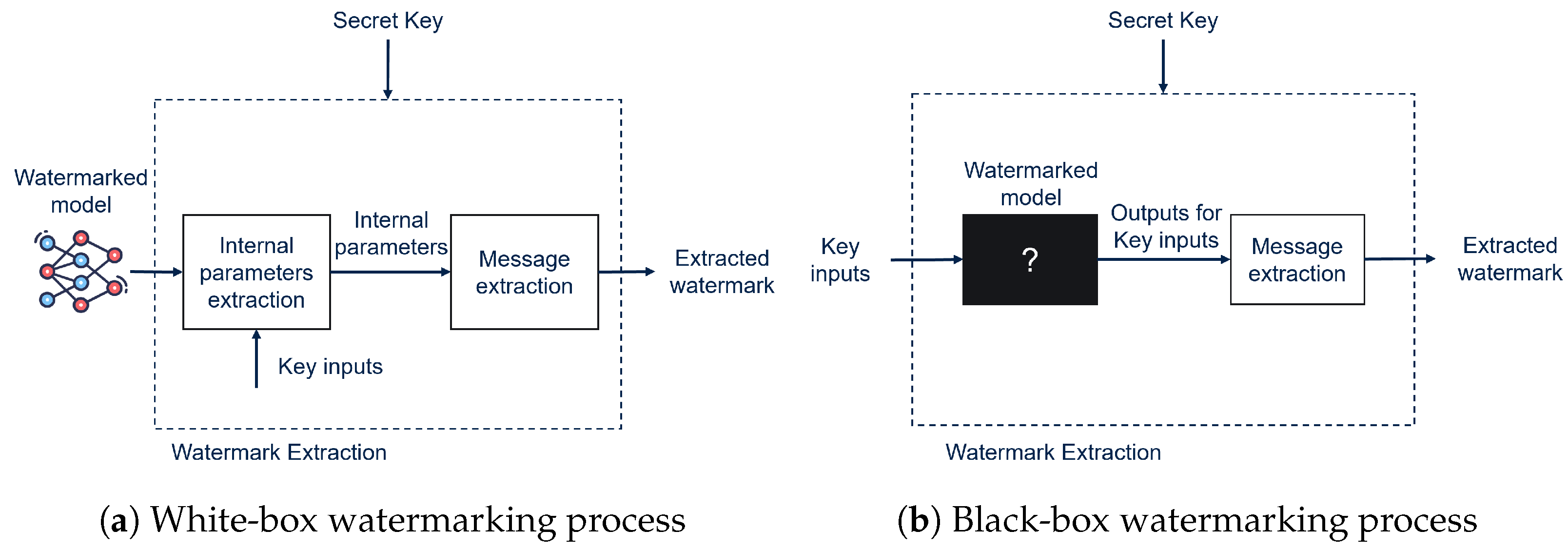

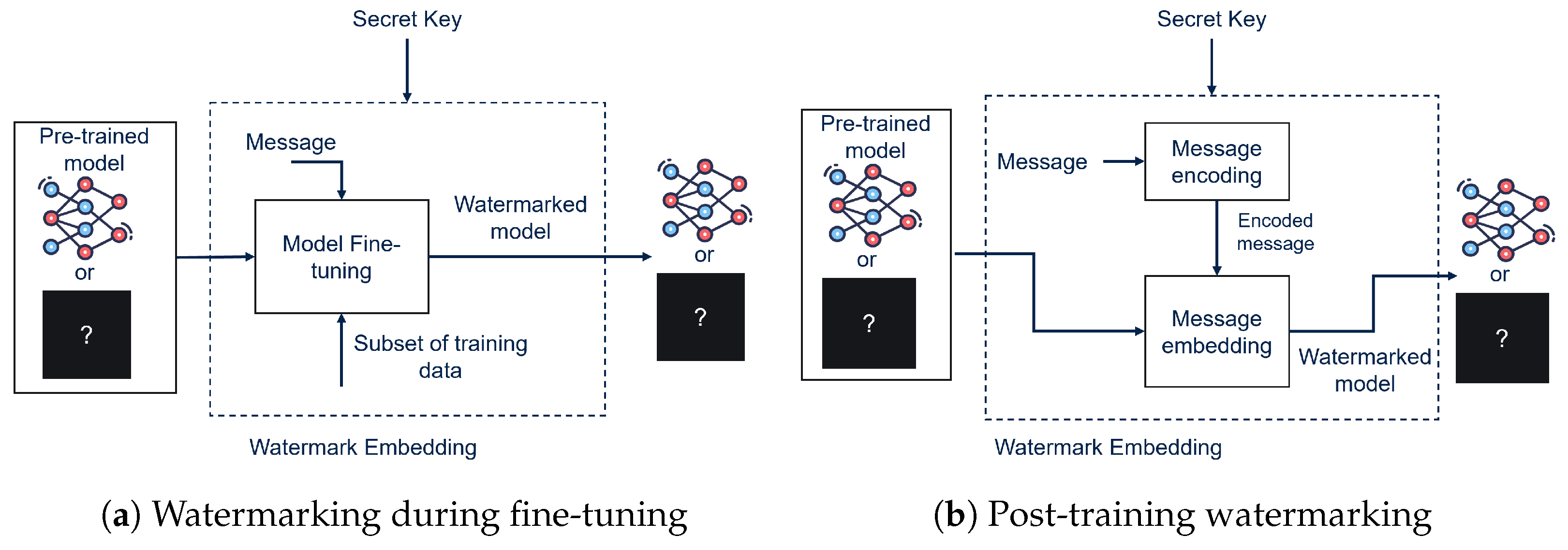
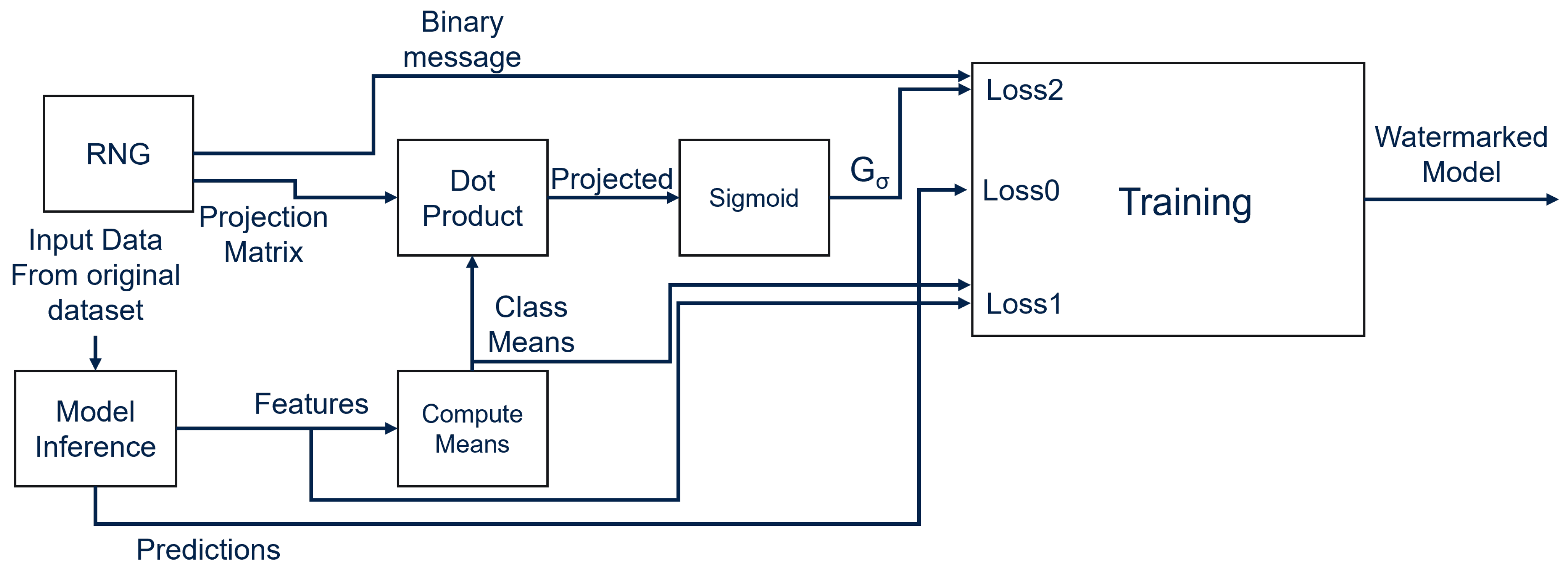
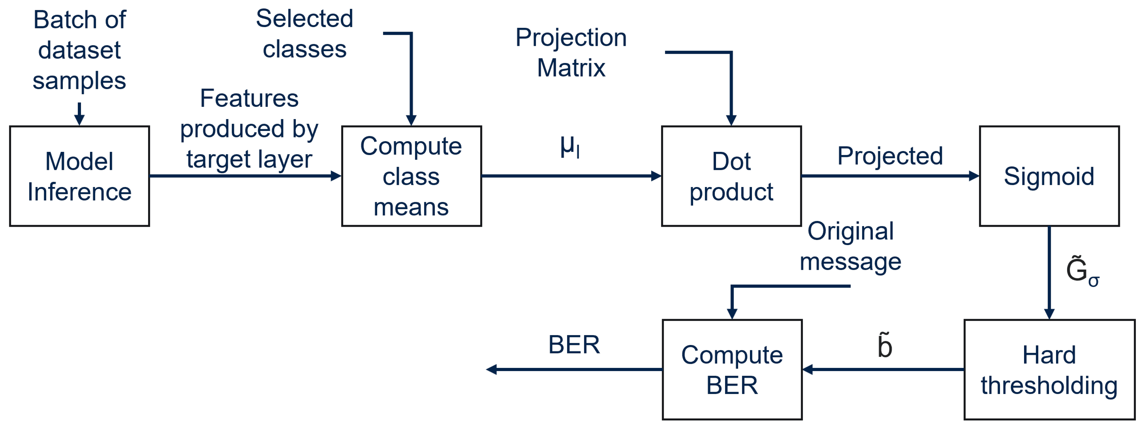

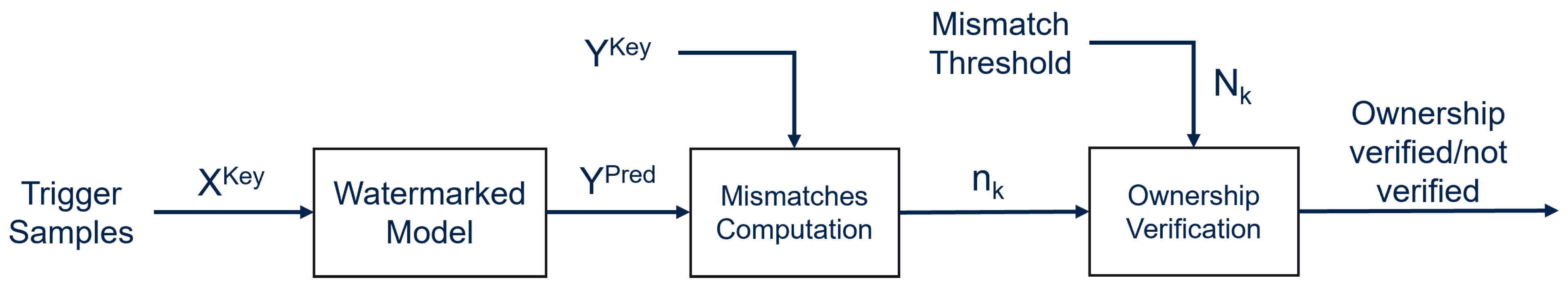
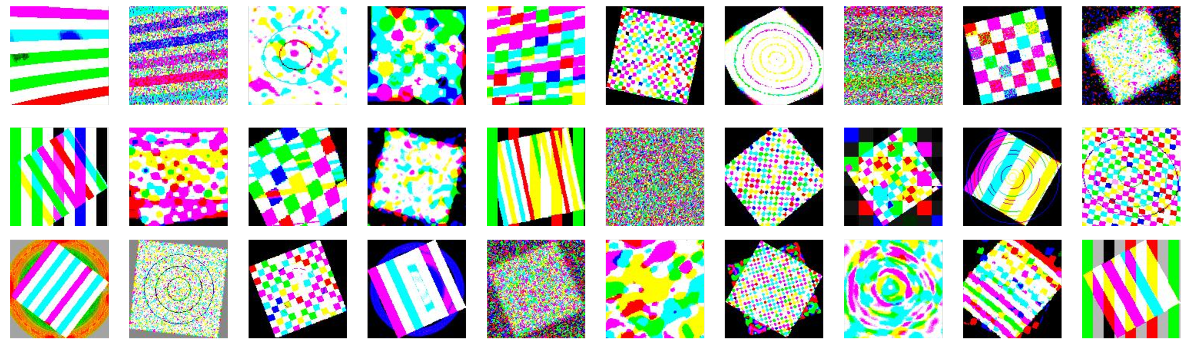
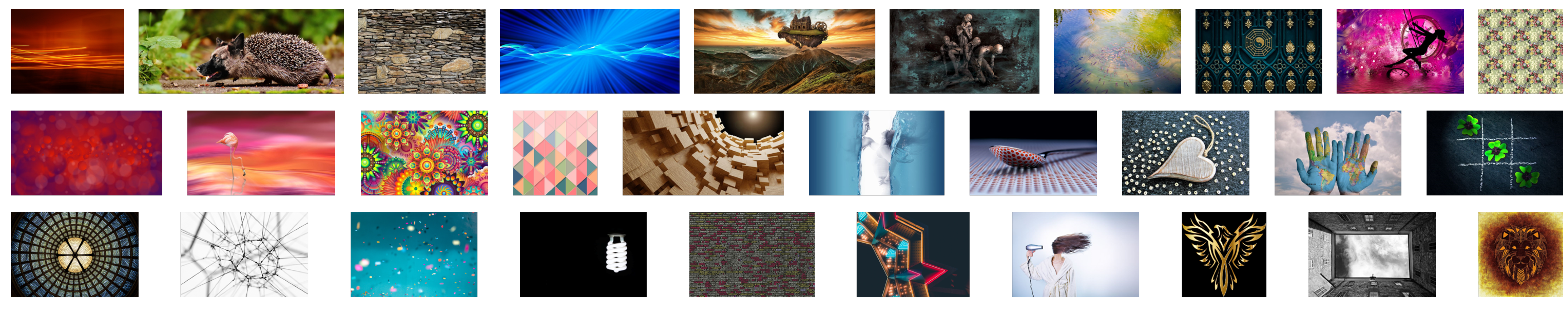
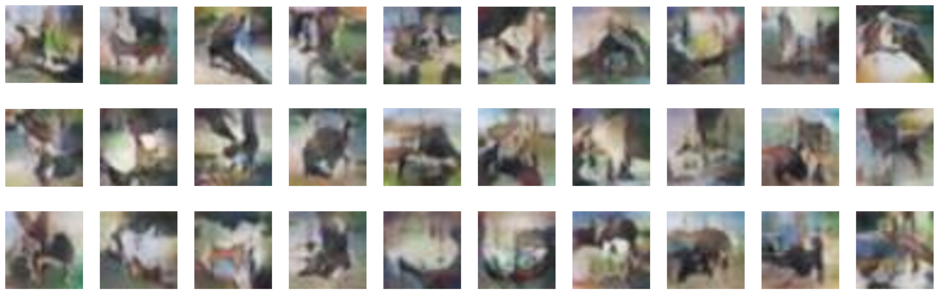
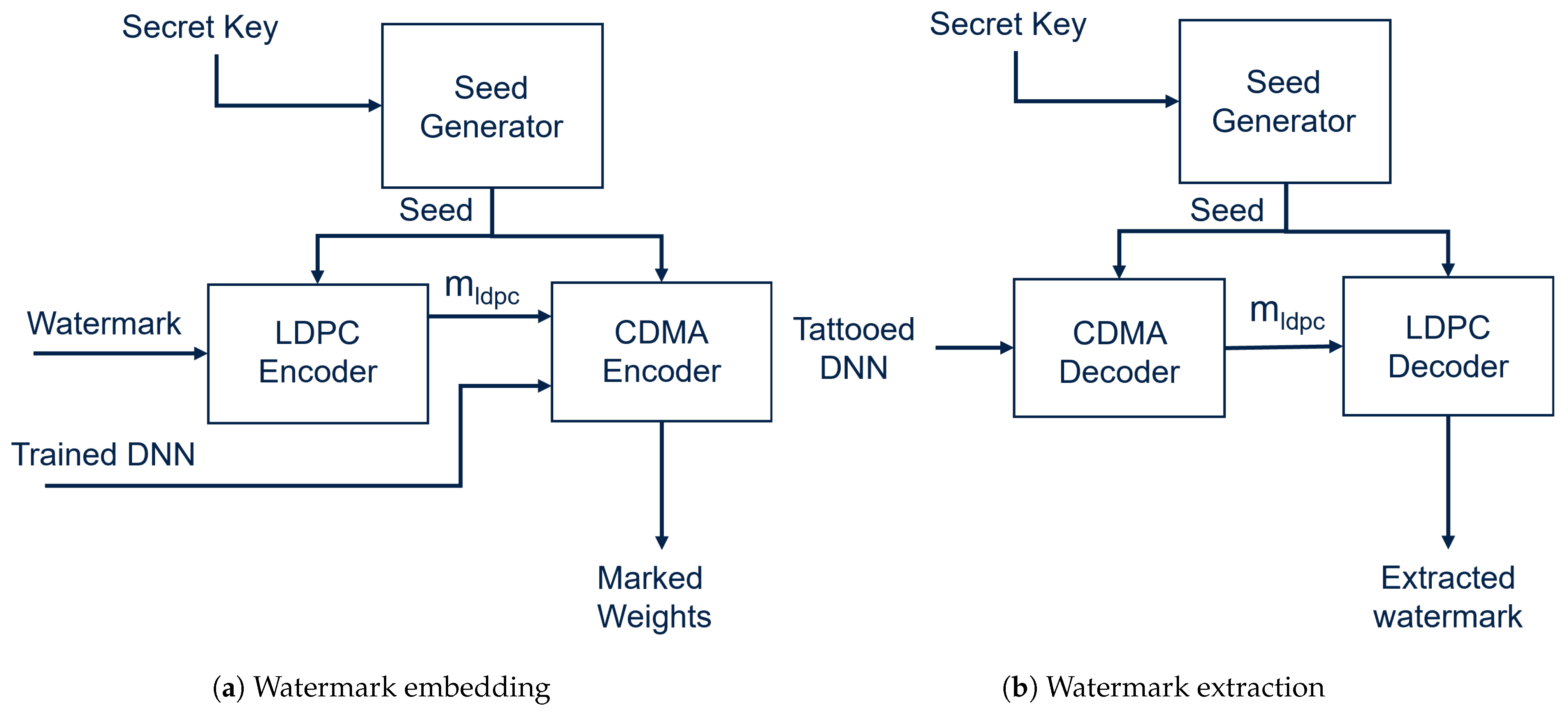
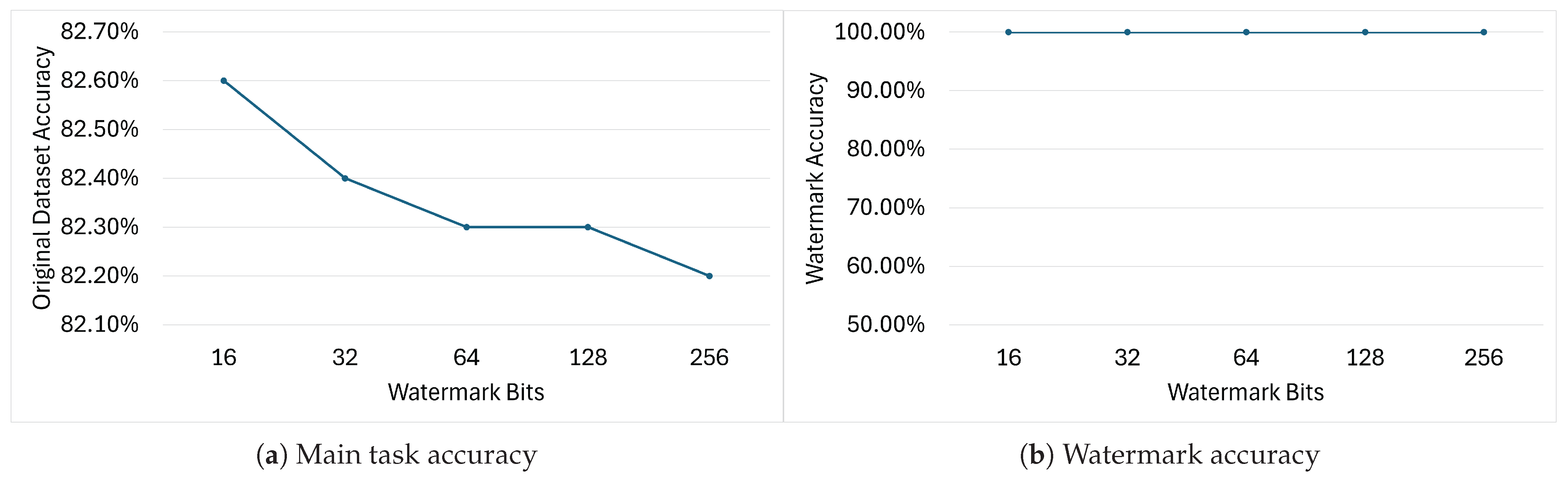
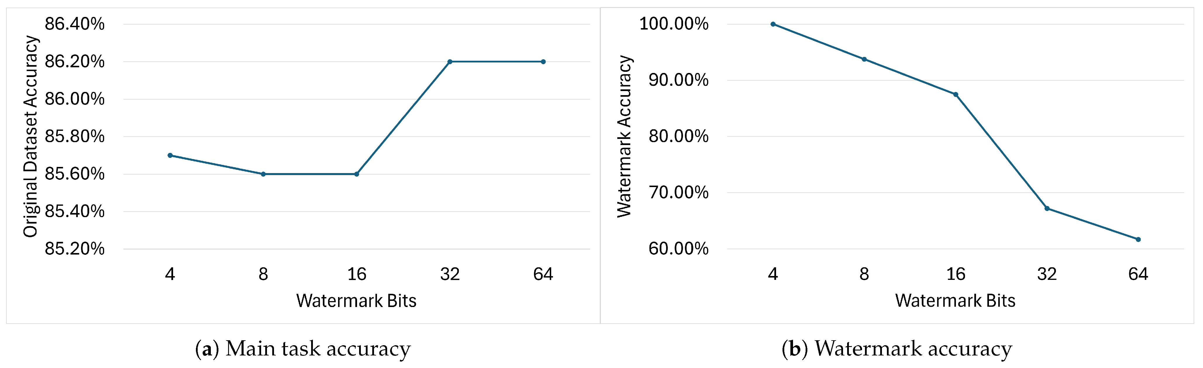

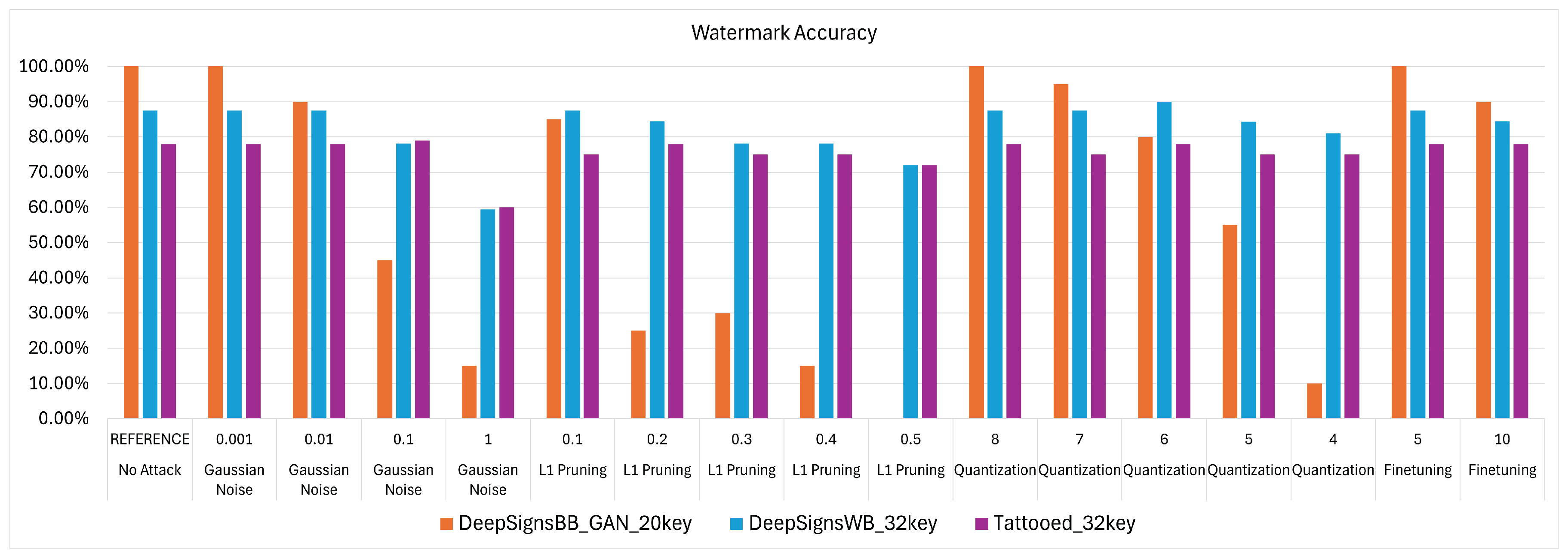
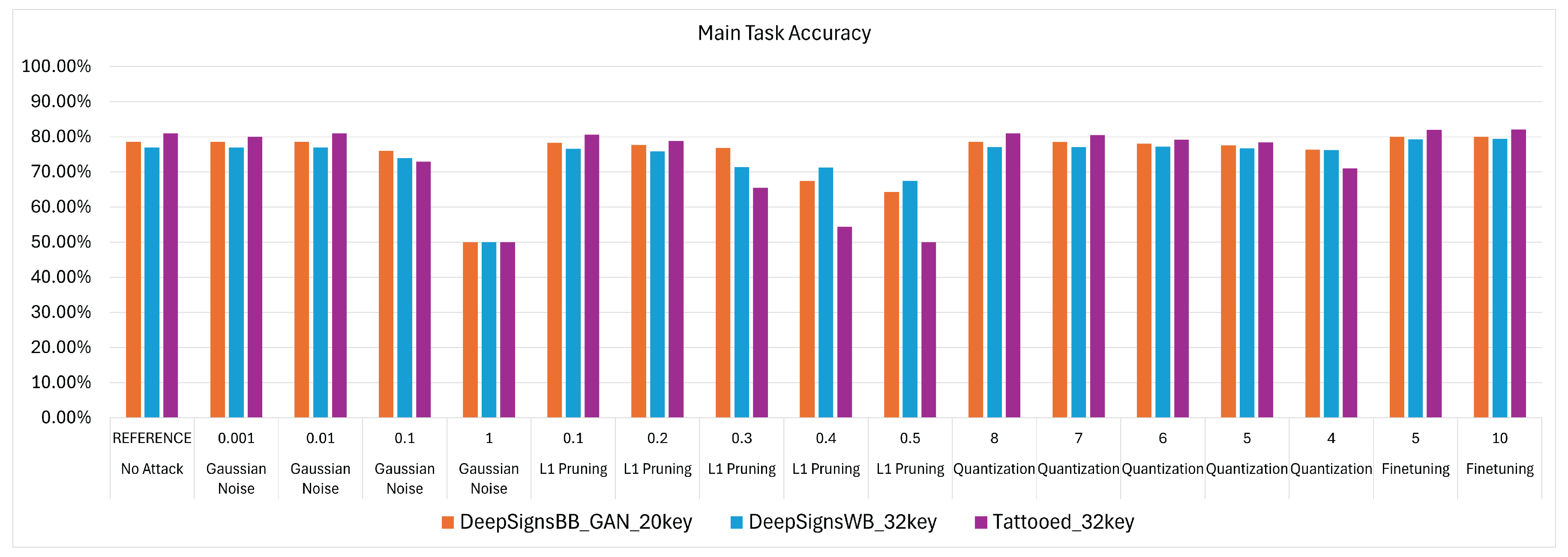

