More Details on Two Solutions with Ordered Sequences for Binomial Confidence Intervals

Abstract

While many continuous distributions are known, the list of discrete ones (usually derived from counting) often reported is relatively short. This list becomes even shorter when dealing with dichotomous observables: binomial, hypergeometric, negative binomial, and uniform. Binomial distribution is important for medical studies, since a finite sample from a population included in a medical study with yes/no outcome resembles a series of independent Bernoulli trials. The problem of calculating the confidence interval (CI, with conventional risk of 5% or otherwise) is revealed to be a problem of combinatorics. Several algorithms dispute the exact calculation, each according to a formal definition of its exactness. For two algorithms, four previously proposed case studies are provided, for sample sizes of 30, 50, 100, 150, and 300. In these cases, at 1% significance level, ordered sequences defining the confidence bounds were generated for two formal definitions. Images of the error’s alternation are provided and discussed. Both algorithms propose symmetric solutions in terms of both CIs and actual coverage probabilities. The CIs are not symmetric relative to the observed variable, but are mirrored symmetric relative to the middle of the observed variable domain. When comparing the solutions proposed by the algorithms, with the increase in the sample size, the ratio of identical confidence levels is increased and the difference between actual and imposed coverage is shrunk.

1. Introduction

In medical studies, sampling a dichotomous outcome emulates a Bernoulli trial, and the ratio between the desired (positive) outcome (x) and the number of trials (or sample size, m) leads to a proportion ($0\le x/m\le 1$). This is a sampling with replacement. The sampling strategy is foundational when dealing with finite populations. In sampling with replacement, after extracting an individual (or a case) from a population, it can be selected for insertion again, having a non-zero probability of being extracted again in the future, while sampling without replacement does not turn it back in the population.

The statistical experiment is as follows: taking a bag with green and yellow balls, we draw out and back in from the bag m balls (the sample), and count how many x are green (Figure 1).

In Figure 1 are illustrated a bag full of balls and a bag half full, after extraction of some of its balls. In a sampling with replacement, the bag is always full, since each ball extracted is immediately returned to the bag. This is the binomial experiment. On the other side, sampling without replacement takes the balls from the bag without returning them in it. Even if the outcome of the two side-by-side experiments may look the same (at the end of the extraction, in both instances x green and $m-x$ yellow balls may be recorded, the experiments are in fact different, and their associated statistics are different too. For instance, a sampling without replacement, if continued indefinitely, will exhaust the balls from the bag, while sampling with replacement will not, even if in the beginning, there are, for example, only two balls in the bag.

There usually is no counting function providing the total number of the balls in the bag (finite or not). To the question “How many green balls (x) out of m will be extracted if the experiment is repeated?”, the result can be expressed using a confidence interval (CI) assuming a success rate (the rate of success is usually 95%).

Fundamental in this context is the probability associated with the reproduction of the observed outcome ($f_{B2}$ in Equation (1)).

$$f_{\mathrm{B}2}(y;x,m,n)=\left({\displaystyle \genfrac{}{}{0pt}{}{n}{y}}\right){\left({\displaystyle \frac{x}{m}}\right)}^y{\left(1-{\displaystyle \frac{x}{m}}\right)}^{n-y}$$

(1)

where ($y,n$) is the second sampling with replacement experiment, while ($x,m$) is the first.

Imposing the size of the second sample at the value of the first one ($n\leftarrow m$), Equation (1) changes to Equation (2):

$$f_{\mathrm{B}}(y;x,m)=f_{\mathrm{B}2}(y;x,m,m)=\left({\displaystyle \genfrac{}{}{0pt}{}{m}{y}}\right){\left({\displaystyle \frac{x}{m}}\right)}^y{\left(1-{\displaystyle \frac{x}{m}}\right)}^{m-y}$$

(2)

In Equations (1) and (2), the true proportion rate (from the population) has been replaced by the observed value of it (from the sample). All information from the sampling has been used and no more information is available, so, Equations (1) and (2) define sufficient statistics.

In layman’s terms, one will never know what is to come from a draw or a sampling in the case of sampling with replacement. A resampling of size m will have a variable number of successes y. However, Equation (2) defines a probability mass function—it is easy to check that Equation (2) is the ($y+1$)-th term from binomial expansion (Equation (3)).

$${\left({\displaystyle \frac{x}{m}}+{\displaystyle \frac{m-x}{m}}\right)}^m=\sum _{y=0}^m\left({\displaystyle \genfrac{}{}{0pt}{}{m}{y}}\right){\left({\displaystyle \frac{x}{m}}\right)}^y{\left(1-{\displaystyle \frac{x}{m}}\right)}^{m-y}$$

(3)

With Equation (2), a CI supporting the drawing y successes from m trials could be constructed around the y value.

The first approach to binomial CI can be attributed to Clopper and Pearson ($C{I}_{\mathrm{CP}}$ in Equation (4)), where the problem was seen as providing an open interval $(p_1,p_2)$ for an observed $p=x/m$, the proportion of units x from a sample of m randomly drawn from a very large population [1]. However, the major limitation of their proposed method is that they give equal weights to the tails, which symmetrizes the confidence interval, making it more intuitive, but biased in the case of binomial. The second disadvantage is that it is expressed from a simple summation of the probabilities from the tails. Lastly, the third disadvantage is that it is expressed via an analytical formula from a continuous distribution (Equation (4)).

$$\begin{array}{cc}\hfill & C{I}_{\mathrm{CP}}(x;m,\alpha ,c_1,c_2)=\hfill \\ \hfill & \left({\left(1+{\displaystyle \frac{m-x+c_2}{x+c_1}}{\mathcal{F}}_{1-\alpha }^{-1}(2(m-x+c_2),2(x+c_1))\right)}^{-1},{\left(1+{\displaystyle \frac{m-x+c_1}{x+c_2}}{\mathcal{F}}_{1-\alpha }^{-1}(2(x+c_2),2(m-x+c_1))\right)}^{-1}\right)\hfill \end{array}$$

(4)

where $\mathcal{F}$ is Fisher’s distribution (the same can be expressed using Beta distribution), with $c_1=0$ and $c_2=1$.

Other alternatives were explored as well. Jeffreys [2] takes different values for the two constants: $c_1=0.5$ and $c_2=0.5$. One can imagine such many corrections. However, the main problem is still unsolved: all of those are patches, and none of those is optimal.

One major progress was made by Casella [3], which proposed refining of the CI by using algorithms instead of mathematical formulas. The solutions proposed here differ from the one proposed by Casella. Here, it is admitted that there is no ideal solution, only optimal ones, when the optimality condition needs to be specified.

2. Background

In the case of continuous distribution functions, the cumulative distribution function has an inverse, and a calculable CI is extracted from it. Fisher called this case fiducial [4].

Calculating the CI (with conventional risk of 5% or otherwise) for a discrete probability distribution is a problem of combinatorics, fact recognized since the beginning [1] but the complexity of the problem denied the availability of an exact method for its calculation until much later [5].

Discrete distribution functions play an important role in statistics. Take, for instance, the uniform discrete distribution, which is at the foundation of any random number generator [6]. The Poisson distribution often serves to provide a size for a sample to be drawn [7,8], while binomial and negative binomial distributions are twin correspondences of Gaussian and Gamma distributions [9,10].

To estimate the CI for a binomial distribution, a series of approximations has been proposed, speculating the normal asymptotic behavior of the binomial distribution [11,12,13,14,15,16]. The construction of exact intervals has been proposed as well [5,17,18,19,20].

3. From Wald’s to Binomial CI

In many ways, Wald’s CI [11], derived under the assumption of an infinite population, is a scholastic example of a CI.

Let us take an example, $z_{\alpha }=\Phi (1-\alpha /2)$, where $\Phi$ is the cumulative function of the normal distribution. For $\alpha$ = 0.01 $,z_{\alpha }$ is about 2.57583. A Wald CI [11] will be calculated by Equation (5).

$$C{I}_{Wald}(x,m,\alpha )=x\pm z_{\alpha }\sqrt{x(m-x)/m}$$

(5)

However, this interval makes no sense with boundaries smaller than 0 or larger than m. Furthermore, any non-integer value of the boundary makes no difference, since x takes only integer values.

A CI for binomial distribution should be seen as the outcome of an algorithm rather than of an simple mathematical formula.

The outcome of such an algorithm is a series of numbers, indexed from 0 to m: $N_0,N_1\dots ,N_m$. By symmetry, a CI should be constructed with these numbers for x out of m as a closed interval, as in Equation (6).

$$C{I}_{OIS}(x,m,\alpha )=[N_x,m-N_{m-x}]$$

(6)

where $N_0,\dots ,N_m$ depends on $\alpha$, but their dependence was not explicitated for the sake of simplification. The construction of $[N_x,m-N_{m-x}]$ should be made in a manner in which always $x\in [N_x,m-N_{m-x}]$ (or in a more convenient notation $N_x\le x\le m-N_{m-x}$).

In Equation (5), the symmetry is realized around x ($C{I}_{WaldL}(x,m,\alpha )$ + $C{I}_{WaldU}(x,m,\alpha )$ = $2x$), while in Equation (7), the antisymmetry is realized around m ($N_x+N_{m-x}=m$). This is a major transformation. However, in some instances, some simple functions can be used for the change.

One can try to apply the percepts of Equation (6) on the values provided by Equation (5). If $C{I}_{Wald}$ (Equation (5)) is expressed by its boundaries $C{I}_{WaldL}$ and $C{I}_{WaldU}$ (as a closed interval, $[C{I}_{WaldL},C{I}_{WaldU}]$), then symmetrization of it imposes the transformations given in Equation (7).

$$\begin{array}{c}\hfill C{I}_{WS}(x,m,\alpha )=[\lceil \max (C{I}_{WaldL}(x,m,\alpha ),0)\rceil ,\lfloor \min (C{I}_{WaldU}(x,m,\alpha ),m)\rfloor ]\end{array}$$

(7)

In Equation (7), the antisymmetry is realized with ceil ($\lceil ·\rceil$ and floor ($\lfloor ·\rfloor$) functions along with max and min. However, the solutions provided by Equation (7) are not optimal.

Table 1. From Wald’s ($C{I}_W$) to binomial ($C{I}_{WS}=[C{I}_{WSL},C{I}_{WSU}]$) CIs (case at $m=9$ and $\alpha =1\%$).

x	$\mathit{x}\pm {\mathit{CI}}_{\mathit{W}}$	${\mathit{CI}}_{\mathit{WS}}$	${\mathit{N}}_{\mathit{x}}$ and ${\mathit{N}}_{9-\mathit{x}}$	p
0	$0\pm 0.00$	[0, 0]	$N_0=0$; $9-N_{9-0}=0\Rightarrow N_9=9$	0.00%
1	$1\pm 2.43$	[0, 3]	$N_1=0$; $9-N_{9-1}=3\Rightarrow N_8=6$	1.21%
2	$2\pm 3.21$	[0, 5]	$N_2=0$; $9-N_{9-2}=5\Rightarrow N_7=4$	0.54%
3	$3\pm 3.64$	[0, 6]	$N_3=0$; $9-N_{9-3}=6\Rightarrow N_6=3$	0.83%
4	$4\pm 3.84$	[1, 7]	$N_4=1$; $9-N_{9-4}=7\Rightarrow N_5=2$	1.33%
5	$5\pm 3.84$	[2, 8]	$N_5=2$; $9-N_{9-5}=8\Rightarrow N_4=1$	1.33%
6	$6\pm 3.64$	[3, 9]	$N_6=3$; $9-N_{9-6}=9\Rightarrow N_3=0$	0.83%
7	$7\pm 3.21$	[4, 9]	$N_7=4$; $9-N_{9-7}=9\Rightarrow N_2=0$	0.54%
8	$8\pm 2.43$	[6, 9]	$N_8=6$; $9-N_{9-8}=9\Rightarrow N_1=0$	1.21%
9	$9\pm 0.00$	[9, 9]	$N_9=9$; $9-N_{9-9}=9\Rightarrow N_0=0$	0.00%

contains CIs calculated with Equation (5), their transformation into ordered numbers series as in Equation (6), and their coverage probabilities.

The p-value listed in Table 1 is the actual non-coverage probability. One can expect the value of p to be identical with imposed coverage probability ($\alpha$). However, it is possible to achieve this coincidence only for continuous distributions. In the case of discrete distributions, the actual coverage probability will always oscillate around the imposed value, and this is the central piece of the problem: how to construct the confidence interval to have the best agreement between the imposed and actual coverages. The solution depends on how the best agreement is defined.

Table 1 lists CIs for the binomial variables (x in Table 1) with nonnegative integers as boundaries.

One should notice the symmetry in the intervals provided in Table 1. The solution provided in Table 1 is not optimal. Thus,

• If it is optimal to provide an at least $1-\alpha$ coverage, then $C{I}_{WS}(1,9,0.01)$ should be [0, 4] instead of [0, 3], with a coverage of 99.86% instead of 98.79% and $C{I}_{WS}(8,9,0.01)$ should be [5, 9] instead of [6, 9], with a coverage of 99.86% instead of 98.79%; $C{I}_{WS}(4,9,0.01)$ should be [0, 7] instead of [1, 7], and $C{I}_{WS}(5,9,0.01)$ should be [0, 7] instead of [1, 7], each with a coverage of 95.27% and 96.12% instead of 92.44%;
• If it is optimal to provide an at most $1-\alpha$ coverage, then $C{I}_{WS}(2,9,0.01)$ should be [0, 4] instead of [0, 5], and $CI(7,9,0.01)$ should be [3, 9] instead of [4, 9], each with a coverage of 96.96% instead of 99.46%; $CI(3,9,0.01)$ should be [0, 5] or [1, 6] instead of [0, 6], and $CI(6,9,0.01)$ should be [4, 9] or [3, 8] instead of [3, 9], with a coverage of 95.76% or 96.57% instead of 99.17%;
• As it can be observed, imposing a single rule (such as “at least” or “at most”) is not enough—see alternatives for $CI(3,9,0.01)$ and $CI(6,9,0.01)$, where further action is to decide among two alternatives; in this instance, the closest one can be picked;
• If it is optimal to provide the closest coverage to the imposed, then $C{I}_{WS}(4,9,0.01)$ would be [0, 7] and $C{I}_{WS}(5,9,0.01)$ would be [2, 9], each with a 99.92% coverage instead of 98.67%;
• To be closest to the imposed coverage but at least equal to or at most equal to seems reasonable criteria as well.

The example given in Table 1 as well as the discussion from above clearly indicates that there is no unique recipe for an ideal CI for binomial distribution. There are many optimal solutions, depending on what is considered to be optimal.

A CI provided by a mathematical formula correcting another mathematical formula, such as Agresti–Coull [14] and Wilson [12], will only chop the interval, without regard to the associated probabilities. Furthermore, this applicability is limited to $\alpha =0.05$ imposed non-coverage error.

4. Algorithms for an Exact Calculation of the Binomial CIs

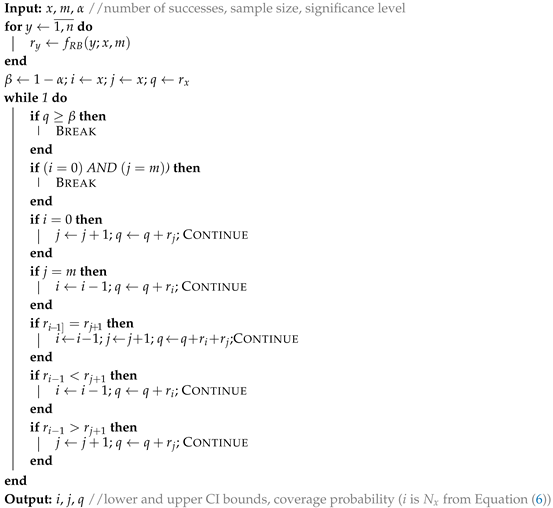
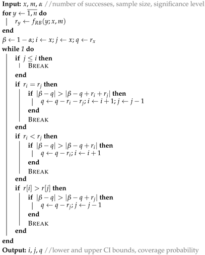
One should change the way in which one constructs a CI for a discrete distribution. In the case of binomial distribution, a mathematical formula is not able to encompass the complexity of the issue. Three algorithms have been proposed in [21]. In this instance, for two of the algorithms (out of three), simplified versions are considered (a best balanced and a best conservative), and their solutions are discussed.

In the following descriptions, $\alpha$ is the imposed level, x is the number of successes, m is the number of trials, $[i,j]$ is the CI, and q is its actual coverage.

The differences between the algorithms are as follows. Algorithm 1 systematically keeps the error below the imposed level, while Algorithm 2 systematicaly keeps the error closest to the imposed level. There is a symmetry in the CIs provided by both algorithms. Their general form is $[N_x,m-N_{m-x}]$, where m is the sample size and $x=0,1,\dots ,m$. Some $N_x$ series are listed in the Section 8 (Raw Data) for the following case studies. The $N_x$ series are monotonic for Algorithm 2, while they are not for Algorithm 1. As an effect of the simplified design of the CIs, which are mirrored relatively to the middle, the actual coverage probabilities series are also symmetric.

Algorithms 1 and 2 have great generality. By summing the probabilities of the events left out and summing the probabilities of the events included, Algorithm 2 provides the interval as the closest solution to the imposed level $\alpha$. By summing the probabilities of the events left out and summing the probabilities of the events included, Algorithm 1 provides the interval as the closest solution to the imposed level $\alpha$ under the specified constraint - the sum of the probabilities for the events left out is at most equal with the imposed level. One can feed Algorithms 1 and 2 with arbitrary values for x, m, and $\alpha$ (under the usual constraints, $0\le x\le m$, $2\le m$, $x,m\in \mathbb{N}$, and $\alpha \in (0,1)$, and even the analytical function $f_{RB}(y;x,m)$), without change to the outcome of the algorithms (the closest solution to the imposed level $\alpha$ without (Algorithm 2) or with (Algorithm 1) constraint regarding the sum of probabilities of events left out).

Algorithm 1: Conservative.

Algorithm 2: Balanced.

5. Case Studies

The CIs, designed CI2 (from Algorithm 2) and CI3 (from Algorithm 1), are calculable for any selection of $\alpha$ ($0<\alpha <1$), m ($1<m$), and x ($0\le x\le m$). However, differences between their outputs are significant for small sample sizes m. Two small ($m=30$ and $m=45$), one medium ($m=100$), and one big ($m=900$) sample sizes were chosen as case studies. For those samples, at significance level $\alpha =1\%$ (the risk of being in error), the CIs were generated.

One would ask which is the error rate if CI is obtained using other approaches. The answer to this question is shortly provided for the following cases, taking into consideration that, when one event is failed to be included in the coverage interval, the error is considered to be of type I (false positive, erroneous rejection). When one event is erroneously included in the coverage interval, then the error is considered to be of type II (false negative, erroneous failure).

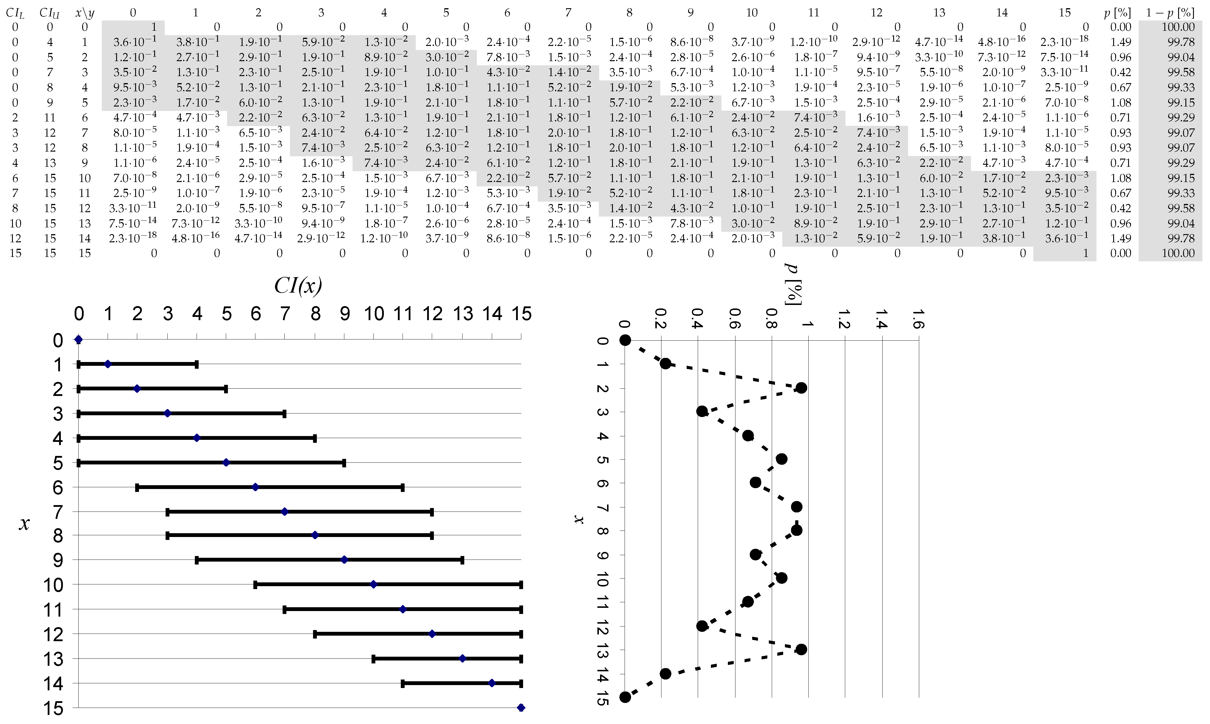
5.1. Case Study 1: m = 15

The $N_x$ values constructing CIs (as $[N_x,15-N_{15-x}]$) are given in the Appendix at $m=15$ entry ($N_0$, …, $N_{15}$). Figure 2 and Figure 3 below are given to illustrate the way in which the CI is constructed. At any number of successes x, the CI contains x, but unlike Wald’s CI, the borders are at not equal distance from x.

It can be observed in Figure 2 and Figure 3 that the CI is shortest at the ends of the domain (at $x=0$ and $x=m$), and is increasing monotonically in width until the middle (at $x=m/2$ for x even and at $x=(m\pm 1)/2$ for x odd), where it reaches its maximum width. The same behavior is for any value of m and $\alpha$.

The shaded parts in Figure 2 and Figure 3 represent the series of y values included in the confidence interval, while $1-p$ (shaded too) is its actual coverage probability (which is the sum of the individual probabilities shaded in its row). The increase in $1-p$ is caused by enlarging the CI, while the decreasing of it (by adding one unit wherever possible at its ends) is caused by the shrinking of it (by substracting one unit wherever possible at its ends).

There are differences between solutions proposed by Algorithms 1 and 2. The coverage of CI proposed by Algorithm 1 is always at least equal with the imposed level. Thus, if CI(1,15,0.01) with Algorithm 2 is [0, 3], with Algorithm 1, it is [0, 4]. The same can be said for CI(14,15,0.01). The enlarged CI from Algorithm 2 to Algorithm 1 is for $x=5$ (from [1, 9] to [0, 9]) and $x=10$ (from [6, 14] to [6, 15]) too. The CI proposed by Algorithm 1 is always equal or contains the CI proposed by Algorithm 2. There are 11 (out of 16, 68.75%) common $N_x$ values ($N_0$, $N_2$, $N_3$, $N_4$, $N_6$, $N_7$, $N_8$, $N_9$, $N_{11}$, $N_{12}$, $N_{13}$, and $N_{15}$).

If one uses Equation (5) instead of Algorithm 2, a number of 5 events will not be included in the CI, while another 5 will be omitted to be included, giving a total error rate of 8.77% (114 events are to be included in total). If one uses Equation (5) instead of Algorithm 1, a number of 7 events will not be included in the CI, while another 7 will be omitted to be included, giving a total error rate of 11.86% (118 events are to be included in total). Furthermore, in this instance, in 10 cases, the CI provided has a coverage smaller than the one imposed by the significance level, providing an error rate of 62.5% (there are 16 cases in total).

5.2. Case Study 2: m = 30

The $N_x$ values constructing CIs (as $[N_x,30-N_{30-x}]$) are given in the Appendix at $m=30$ entry ($N_0$, …, $N_{30}$). The plot of actual non-coverage probabilities is given in Figure 4.

The alternative proposed by Algorithm 2 on Figure 4 jumps below and above the imposed level of 1%, with the smallest deviation to it, while the one proposed by Algorithm 1 on Figure 4 is visible below the imposed level of 1%, being the closest choice to it. There are 13 (out of 31, 41.94%) common $N_x$ values ($N_0$, $N_3$, $N_7$, $N_9$, $N_{12}$, $N_{13}$, $N_{15}$, $N_{17}$, $N_{18}$, $N_{21}$, $N_{23}$, $N_{27}$, and $N_{30}$).

If one uses Equation (5) instead of Algorithm 2, a number of 9 events will not be included in the CI, while another 9 will be omitted to be included, giving a total error rate of 5.57% (323 events are to be included in total). If one uses Equation (5) instead of Algorithm 1, a number of 16 events will not be included in the CI, while another 16 will be omitted to be included, giving a total error rate of 9.38% (341 events are to be included in total). Furthermore, in this instance, in 22 cases, the CI provided has a coverage smaller than the one imposed by the significance level, providing an error rate of 71.0% (there are 31 cases in total).

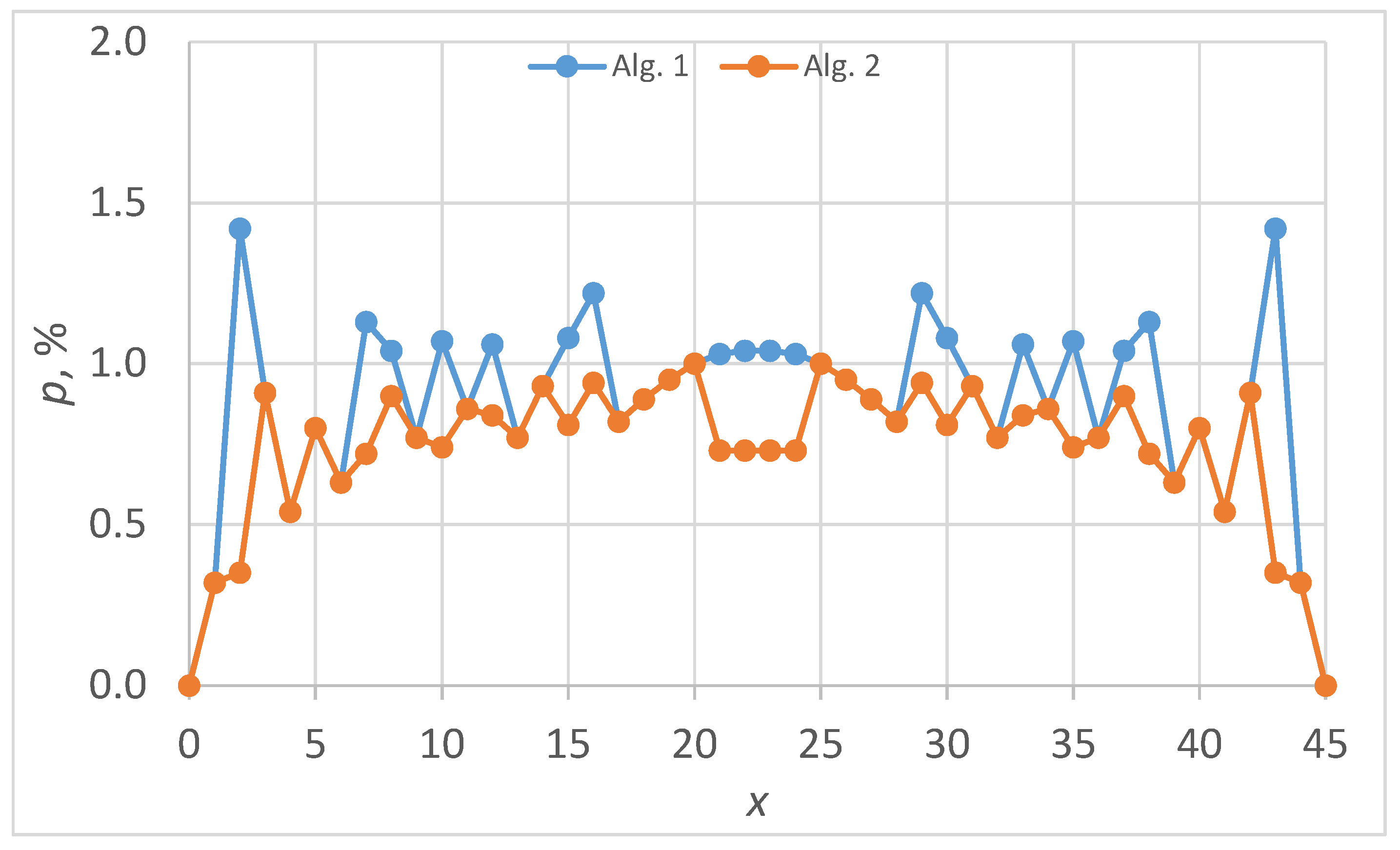
5.3. Case Study 2: m = 45

The $N_x$ values constructing CIs (as $[N_x,45-N_{45-x}]$) are given in the Appendix at $m=45$ entry ($N_0$, …, $N_{45}$). The plot of actual non-coverage probabilities is given in Figure 5.

The alternative proposed by Algorithm 2 on Figure 4 jumps below and above the imposed level of 1%, with the smallest deviation to it, while the one proposed by Algorithm 1 on Figure 4 is visible below the imposed level of 1%, being the closest choice to it. There are 24 (out of 46, 52.20%) common $N_x$ values.

If one use Equation (5) instead of Algorithm 2, a number of 15 events will not be included in the CI, while another 15 will be omitted to be included, giving a total error rate of 4.97% (604 events are to be included in total). If one use Equation (5) instead of Algorithm 1, a number of 22 events will not be included in the CI, while another 22 will be omitted to be included, giving a total error rate of 7.07% (622 events are to be included in total). Furthermore, in this instance, in 19 cases, the CI provided has a coverage smaller than the one imposed by the significance level, providing an error rate of 41.3% (there are 46 cases in total).

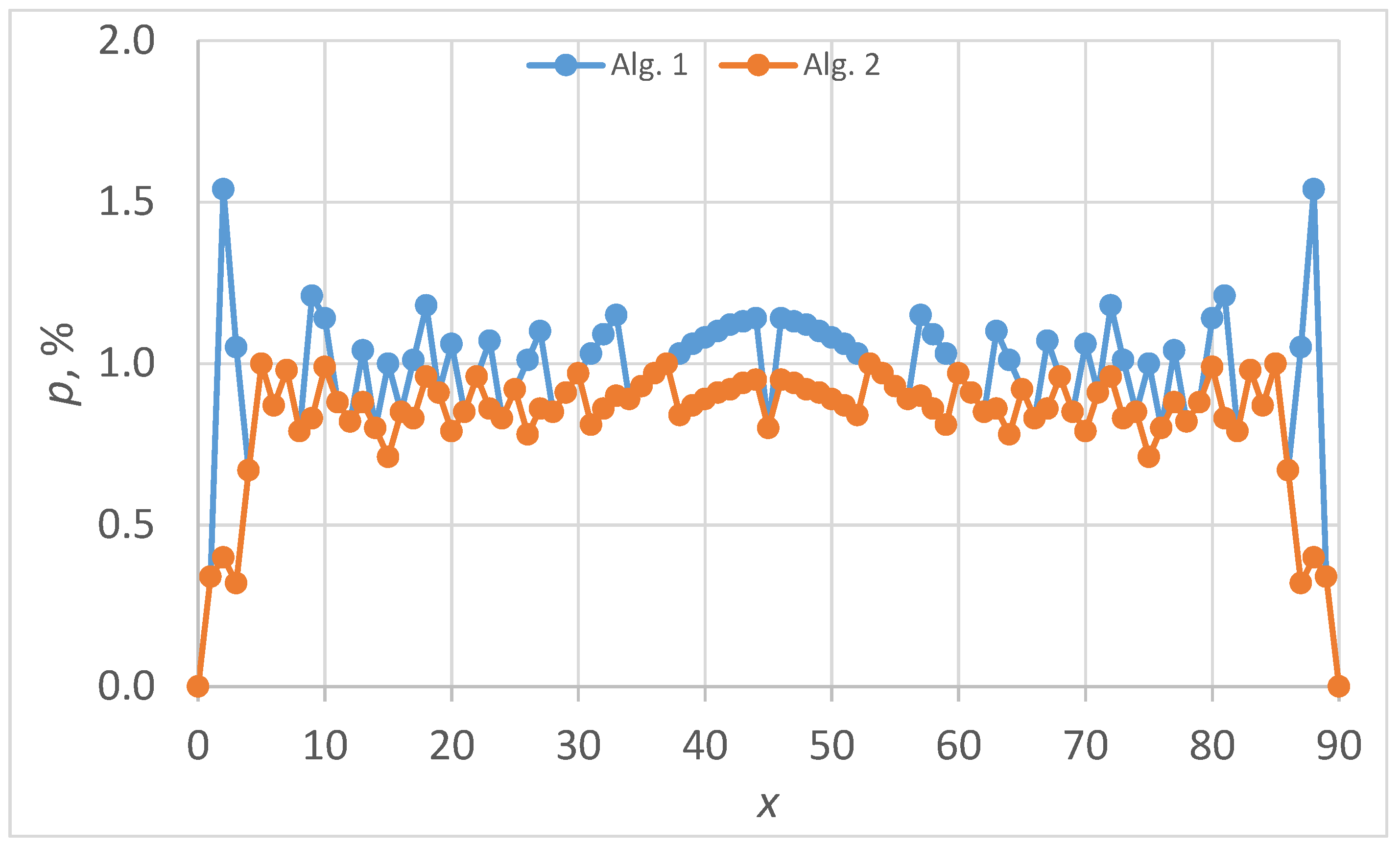
5.4. Case Study 3: m = 90

The $N_x$ values constructing CIs (as $[N_x,90-N_{90-x}]$) are given in the Appendix at $m=90$ entry ($N_0$, …, $N_{90}$). The plot of actual non-coverage probabilities is given in Figure 6.

The alternative proposed by Algorithm 2 on Figure 4 jumps below and above the imposed level of 1%, with the smallest deviation to it, while the one proposed by Algorithm 1 on Figure 4 is visible below the imposed level of 1%, being the closest choice to it. There are 69 (out of 91, 75.82%) common $N_x$ values.

If one uses Equation (5) instead of Algorithm 2, a number of 34 events will not be included in the CI, while another 34 will be omitted to be included, giving a total error rate of 3.97% (1715 events are to be included in total). If one uses Equation (5) instead of Algorithm 1, a number of 54 events will not be included in the CI, while another 54 will be omitted to be included, giving a total error rate of 6.14% (1759 events are to be included in total). Furthermore, in this instance, in 66 cases, the CI provided has a coverage smaller than the one imposed by the significance level, providing an error rate of 72.5% (there are 91 cases in total).

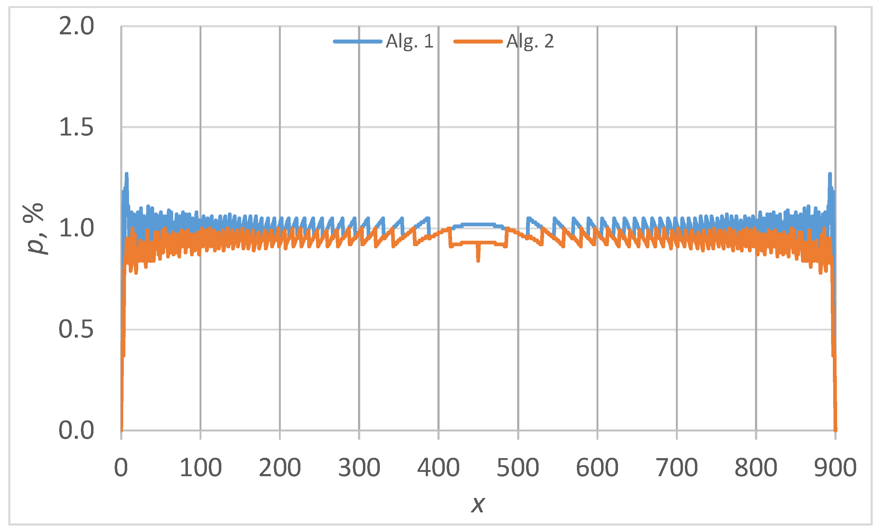
5.5. Case Study 4: m = 900

The values of the numbers constructing the confidence intervals with $[N_x,900-N_{900-x}]$ are given in Section 8 for $m=900$ ($N_0$, …, $N_{900}$). The coverages were obtained with Algorithm 2 for CI2 and Algorithm 1 for CI3. The plot of the actual non-coverage probabilities is given in Figure 7.

The CI2 vs. CI3 distinct points are hardly visible in Figure 7, confirming the tendency in decreasing their proportion.

If one uses Equation (5) instead of Algorithm 2, a number of 282 events will not be included in the CI, while another 282 will be omitted to be included, giving a total error rate of 1.03% (54,577 events are to be included in total). If one uses Equation (5) instead of Algorithm 1, a number of 452 events will not be included in the CI, while another 452 will be omitted to be included, giving a total error rate of 1.70% (55,037 events are to be included in total). Furthermore, in this instance, in 641 cases, the CI provided has a coverage smaller than the one imposed by the significance level, providing an error rate of 71.1% (there are 901 cases in total).

6. Discussion

The two proposed algorithms (Algorithms 1 and 2) work fine, and a series of cases were used to emphasize their behavior. The actual non-coverage probability proposed by Algorithm 2 is closer to the imposed level than the actual non-coverage probability proposed by Algorithm 1 in average. The averages are given in

Table 2. Comparing actual coverage probabilities for selected sample sizes at $\alpha =0.01$.

Sample	Alg.	$\mathit{m}=15$	$\mathit{m}=30$	$\mathit{m}=45$	$\mathit{m}=90$	$\mathit{m}=900$
Averages (%)	Algorithm 2	0.7825	0.9987	0.8817	0.9611	0.9947
	Algorithm 1	0.5950	0.6723	0.7370	0.8240	0.9352
Averages of departures from imposed level (%)	Algorithm 2	0.3600	0.2606	0.2130	0.1418	0.0395
	Algorithm 1	0.4050	0.3277	0.2630	0.1760	0.0648

.

The average of the actual non-coverage is not monotonically convergent to the imposed level (see the value of actual non-coverage for $m=30$ vs. for $m=15$ and $m=45$ from Algorithm 2). The averages for the actual non-coverage provided by the Algorithm 1 are slightly more departed (in average) from the imposed level, the constraint of always being smaller than the imposed level explaining this behavior. The tendency in convergence to the imposed level is with ${\displaystyle \frac{1}{m}}$ (about ${\displaystyle \frac{2.5}{m}}$ for Algorithm 2 CI average coverages and slightly more accelerated for Algorithm 2—about ${\displaystyle \frac{4.1}{m}}$).

One major point is to provide the simplest answers to simple questions. Here are three:

6.1. Question Q1

Are there differences when a different significance level is used?

There definitely are differences at any change of the imposed level of significance. With the increase in $\alpha$, the CI width is decreased. In the following cases, the value of $\alpha$ has been changed to $\alpha =0.05$ (five times bigger risk of being in error).

6.2. Question Q2

Having now two alternatives (Algorithms 1 and 2), which algorithm should be used to express the CI for a binomial variable?

The constraints defined in the algorithms, as well as run results provided in Figure 4, Figure 5, Figure 6 and Figure 7 and Table 2, indicate that Algorithm 2 is suited for the case when the request is to provide a CI with coverage as close as possible to the imposed value. On the other hand, Algorithm 1 is suited for the case when the request is to provide a CI with coverage closest but always at least equal to the imposed value.

6.3. Question Q3

How should one deal with binomial proportions instead of binomial variables?

The main issue is the habit of simplification. For instance, for ${\displaystyle \frac{1}{2}}$, one often writes $0.5$, for ${\displaystyle \frac{1}{3}}$, one writes $0.\left(3\right)$ or $0.33\dots$, but it is, in fact, not the same thing.

The preference for real numbers is obvious—people are much more comfortable with them and they quickly indicate the order of magnitude (0.0… or 0.1… is close to 0, 0.8… or 0.9… is close to 1, 0.4… or 0.5… is close to 0.5), which allows an instant interpretation. At the same time, however, it lets something slip through the cracks. One can express (with three decimal places for example) any real sub-unit number, but its exact value cannot be obtained as a proportion of two integers, except under certain conditions and very few situations (one of these being that the sample size is 1000; for the sample size 997, however, there is no non-trivial situation).

Thus, for $x=16$ positive outcomes from $m=20$ trials, in order to pass along all information, one would firstly need a convention to express the proportion as is, without simplifying it (binomial proportion is then ${\displaystyle \frac{16}{20}}$), and the CI is expressed accordingly with fractions too. For 95% CI, simply using the data given in Section 8, with Algorithm 2, CI is $[{\displaystyle \frac{13}{20}},{\displaystyle \frac{19}{20}}]$ and its actual coverage is 95.63%. Further examples are given in

Table 3. Examples of 95% CI with Algorithms 1 and 2.

x, m	Alg.	$\mathbf{CI}(\mathit{x};\mathit{m})$	$\mathbf{CI}\left(\frac{\mathit{x}}{\mathit{m}}\right)$	$1-\mathit{p}$	${\mathit{N}}_{\mathit{x}}$, ${\mathit{N}}_{\mathit{m}-\mathit{x}}$
19, 50	Algorithm 2	[13, 25]	$\left[{\displaystyle \frac{13}{50}},{\displaystyle \frac{25}{50}}\right]$	94.3%	13, 25
	Algorithm 1	[19, 25]	$\left[{\displaystyle \frac{12}{50}},{\displaystyle \frac{25}{50}}\right]$	95.7%	12, 25
75, 80	Algorithm 2	[71, 78]	$\left[{\displaystyle \frac{71}{80}},{\displaystyle \frac{78}{80}}\right]$	93.65%	71, 2
	Algorithm 1	[70, 78]	$\left[{\displaystyle \frac{70}{80}},{\displaystyle \frac{78}{80}}\right]$	95.28%	70, 2

p: actual coverage.

($N_x$ series given in Section 8).

6.4. Real-World Data Analysis

In [22], a study was conducted with 20 patients subject to dermal regeneration template placement over areas with exposed bone/tendon prior to split-thickness skin grafting, all being confirmed clinically and microbiologically negative for previously treated infection. With non-invasive fluorescence imaging, the bacterial load was identified using a defined threshold in eight out of twenty patients. Out of eight, four developed an infection. Three out of the four infections were positive for Pseudomonas. Based on the study data, the following research questions can be formed (the null hypothesis is that the effect being studied does not exist, and the observation can be merely by chance):

• Q4: Was the detection of the bacterial load with non-invasive fluorescence imaging statistically significant in the group, or can it be asserted as being observed by chance?
• Q5: Was the developing of a bacterial infection a real risk for the patients following the procedure, or can it be asserted as being observed by chance?
• Q6: Was Pseudomonas a real threat for the patients following the procedure, or can it be asserted as being observed by chance?
• Q7: Was the developing of a bacterial infection a real risk for the patients possessing bacterial load detected by non-invasive fluorescence imaging, or can it be asserted as being observed by chance?
• Q8: Was infection with Pseudomonas a real risk for the patients possessing bacterial load detected by non-invasive fluorescence imaging, or can it be asserted as being observed by chance?

Answers are given in

Table 4. Answers to research questions Q4–Q8 at risk of 5% being in error.

Question	Proportion	CI	Is $0\in$ CI?, Answer (p)
Q4	8 out of 20	[4, 12] and [4, 12]	$0\notin$ CI, Yes (3.6%)
Q5	4 out of 20	[1, 7] and [1, 7]	$0\notin$ CI, Yes (4.3%)
Q6	3 out of 20	[1, 6] and [1, 7]	$0\notin$ CI, Yes (6.1% with [1, 6] and 4.5% with [1, 7])
Q7	4 out of 8	[2, 6] and [1, 7]	$0\notin$ CI, Yes (7.0% with [2, 6] and 0.8% with [1, 7])
Q8	3 out of 8	[1, 5] and [0, 5]	Not a definite answer (associated risks: 5.9% and 3.6%) *

Note: CI was calculated with Algorithm 1 and with Algorithm 2. *: If 5.9% is an acceptable risk of being in error, then the CI is [1, 5] and the answer to Q8 is Yes (null hypothesis must be rejected); If 5.9% is not an acceptable risk of being in error, the alternative CI is [0, 5], the answer is No (one cannot assert the infection with Pseudomonas simply based on bacterial load detected by non-invasive fluorescence imaging), having the risk of being in error of 3.6% (and the null hypothesis cannot be rejected).

.

In [23], a survey study collected data from 28,346 cases of abortions performed before the ninth week of pregnancy, of which the MEFEEGO Pack facility was used. On 26 April 2023, the Japanese Ministry of Health, Labour and Welfare approved the use of the medical abortion pill package with the condition that the patient undergoes either hospitalization or outpatient observation at a facility with beds, called MEFEEGO Pack in Japan. This facility was used in 435 cases, with no serious complications. The question (let Q9 be this question) is if the patients with MEFEEGO Pack represented a significant proportion within the sample.

Table 5. Answers to Q9 at different risks of being in error.

Question	Proportion	Alg.	CI	Is $0\in$ CI?, Answer	p
$\alpha =0.05$ (imposed level of 5% risk being in error)
Q9	435 out of 28,346	Algorithm 2	[395, 475]	$0\notin$ CI, Answer: Yes	5%
		Algorithm 1	[394, 475]		4.8%
$\alpha =0.01$ (imposed level of 1% risk being in error)
Q9	435 out of 28,346	Algorithm 2	[383, 489]	$0\notin$ CI, Answer: Yes	0.97%
		Algorithm 1	[383, 489]		0.97%
$\alpha =0.001$ (imposed level of 1‰ risk being in error)
Q9	435 out of 28,346	Algorithm 2	[369, 504]	$0\notin$ CI, Answer: Yes	1.01‰
		Algorithm 1	[369, 505]		0.93‰

summarizes this analysis.

Observation by chance increases slowly with sample size. Thus, at a significance level of 1%,

• 3 out of 9 can be by chance; at 4 out of 9, the null hypothesis that the observation can be merely by chance must be rejected (see Table 1);
• 4 out of 15 can be by chance; at 5 out of 15, the null hypothesis that the observation can be merely by chance must be rejected (see $N_x$ series in Section 8 for $m=15$, Algorithm 2, and $\alpha =0.01$);
• 4 out of 15, 30, 45, of 90, and of 900 can be by chance; at 4 out of 15, 30, 45, of 90, and of 900, the null hypothesis that the observation can be merely by chance must be rejected (see $N_x$ series in Section 8 for Algorithm 2 and $\alpha =0.01$) at $m=15$, $m=30$, $m=45$, $m=90$, and $m=900$;
• For data in Table 5: 4 out of 28,346 can be by chance while at 5 out of 28,346, the null hypothesis that the observation can be merely by chance must be rejected.

Observation by chance increases much faster with significance level. Thus, if at significance level of 5%, 3 out of 28,346 can be by chance while 4 out of 28,346 cannot, at significance level of 1‰, 7 out of 28,346 is still by chance while 8 out of 28,346 is not.

7. Applications

In this section, for a series of data taken from two literature sources, the CIs using the proposed method are calculated in order to provide a clear reproducibility of the results and to make available a comparison with any other existing methods.

In [24], it was communicated that the primary efficacy end point was observed in 135 of 173 patients in the scaffold group and 48 of 88 patients in the angioplasty group. The authors used the Kaplan–Meier estimate [25] to get an absolute difference and its associated 95% CI. Using Algorithm 2, 95% CI for ${\displaystyle \frac{135}{173}}$ in the scaffold group is $\left[{\displaystyle \frac{125}{173}},{\displaystyle \frac{145}{173}}\right]$, with a true non-coverage of 5.3%, while with Algorithm 1, 95% CI is $\left[{\displaystyle \frac{125}{173}},{\displaystyle \frac{146}{173}}\right]$, with a true non-coverage of 4.6%. Using Algorithm 2, 95% CI for ${\displaystyle \frac{48}{88}}$ in the angioplasty group is $\left[{\displaystyle \frac{39}{88}},{\displaystyle \frac{56}{88}}\right]$, with a true non-coverage of 5.5%, while with Algorithm 1, 95% CI is $\left[{\displaystyle \frac{38}{88}},{\displaystyle \frac{56}{88}}\right]$, with a true non-coverage of 4.6%. In the same study [24], it was communicated that the primary safety end point was observed in 165 of 170 patients in the scaffold group and 90 of 90 patients in the angioplasty group. Involving Algorithm 2, 95% CI for ${\displaystyle \frac{165}{170}}$ in the scaffold group is obtained as $\left[{\displaystyle \frac{161}{170}},{\displaystyle \frac{169}{170}}\right]$, with a true non-coverage of 3.6%, while with Algorithm 1, 95% CI is obtained the same. Involving either of Algorithms 1 and 2, 95% CI for ${\displaystyle \frac{165}{170}}$ in the angioplasty group is obtained as $\left[{\displaystyle \frac{170}{170}},{\displaystyle \frac{170}{170}}\right]$, with a true non-coverage of 3.6%, while with Algorithm 1, 95% CI is obtained the same. In all cases, there is no overlap between the CIs of the scaffold and angioplasty groups, so there are statistically significant differences. To get an accurate CI for the difference of the two proportions (excess risk), an algorithm-based method (such as the ones reported in [26]) should be used.

In [27], 3200 women were split into intervention (1593) and control (1607) groups. After assignment, 3195 women remained eligible (1590 in the intervention group and 1605 in the control group). Overall, 3061 live births occurred, with 1536 in the intervention group and 1525 in the control group. A total of 85 severe pneumonia cases were identified in the intervention group of 1498 and 90 severe pneumonia cases in the control group of 1486, as well as 182 pneumonia cases, according to WHO IMCI (World Health Organization Integrated Management of Childhood Illness) guidelines [28] (see also Supplementary Appendix of [27]), in the intervention group of 1498 and 197 in the control group of 1498 (see Figure 2 in [27]). A first concern is if there is a statistical difference in the split between the two groups, calculating CI with Algorithms 1 and 2. Thus, with Algorithm 2,

• For ${\displaystyle \frac{1593}{3200}}$, 95% CI with Algorithm 2 is $\left[{\displaystyle \frac{1538}{3200}},{\displaystyle \frac{1648}{3200}}\right]$, and for ${\displaystyle \frac{1607}{3200}}$, 95% CI is $\left[{\displaystyle \frac{1552}{3200}},{\displaystyle \frac{1662}{3200}}\right]$ with an obvious overlap, so no statistical difference here;
• For ${\displaystyle \frac{1590}{3195}}$, 95% CI with Algorithm 2 is $\left[{\displaystyle \frac{1535}{3195}},{\displaystyle \frac{1645}{3195}}\right]$, and for ${\displaystyle \frac{1605}{3195}}$, 95% CI is $\left[{\displaystyle \frac{1550}{3195}},{\displaystyle \frac{1660}{3195}}\right]$ with an obvious overlap, so no statistical difference here either;
• For ${\displaystyle \frac{1536}{3061}}$, 95% CI with Algorithm 2 is $\left[{\displaystyle \frac{1482}{3061}},{\displaystyle \frac{1589}{3061}}\right]$, and for ${\displaystyle \frac{1525}{3061}}$, 95% CI is $\left[{\displaystyle \frac{1472}{3061}},{\displaystyle \frac{1579}{3061}}\right]$ with an obvious overlap, so no statistical difference here either.

Moreover, with Algorithm 1,

• For ${\displaystyle \frac{1593}{3200}}$, 95% CI with Algorithm 2 is $\left[{\displaystyle \frac{1538}{3200}},{\displaystyle \frac{1648}{3200}}\right]$, and for ${\displaystyle \frac{1607}{3200}}$, 95% CI is $\left[{\displaystyle \frac{1552}{3200}},{\displaystyle \frac{1662}{3200}}\right]$, identical with the one provided by Algorithm 2;
• For ${\displaystyle \frac{1590}{3195}}$, 95% CI with Algorithm 2 is $\left[{\displaystyle \frac{1535}{3195}},{\displaystyle \frac{1645}{3195}}\right]$, and for ${\displaystyle \frac{1605}{3195}}$, 95% CI is $\left[{\displaystyle \frac{1550}{3195}},{\displaystyle \frac{1660}{3195}}\right]$, identical with the one provided by Algorithm 2;
• For ${\displaystyle \frac{1536}{3061}}$, 95% CI with Algorithm 2 is $\left[{\displaystyle \frac{1481}{3061}},{\displaystyle \frac{1589}{3061}}\right]$, and for ${\displaystyle \frac{1525}{3061}}$, 95% CI is $\left[{\displaystyle \frac{1472}{3061}},{\displaystyle \frac{1580}{3061}}\right]$ with an obvious overlap, so no statistical difference here either.

As the results show, for large samples, there is a smaller likelihood that the CI provided by Algorithm 1 and Algorithm 2 is different (in the 2/3 cases above, it was identical). Continuing with the pneumonia cases, ${\displaystyle \frac{85}{1498}}$ have 95% CI with Algorithm 2 as $\left[{\displaystyle \frac{68}{1498}},{\displaystyle \frac{102}{1498}}\right]$, and ${\displaystyle \frac{90}{1486}}$ have 95% CI as $\left[{\displaystyle \frac{73}{1486}},{\displaystyle \frac{108}{1486}}\right]$ and with Algorithm 1 as $\left[{\displaystyle \frac{67}{1498}},{\displaystyle \frac{102}{1498}}\right]$, and ${\displaystyle \frac{90}{1486}}$ have 95% CI as $\left[{\displaystyle \frac{73}{1486}},{\displaystyle \frac{109}{1486}}\right]$. The CIs overlap, so no statistical difference here either. Finally, for pneumonia cases, according to WHO IMCI guidelines, ${\displaystyle \frac{182}{1498}}$ have 95% CI with Algorithm 2 as $\left[{\displaystyle \frac{158}{1498}},{\displaystyle \frac{207}{1498}}\right]$, and ${\displaystyle \frac{197}{1486}}$ have 95% CI as $\left[{\displaystyle \frac{172}{1486}},{\displaystyle \frac{222}{1486}}\right]$, and with Algorithm 1, ${\displaystyle \frac{182}{1498}}$ have 95% CI as $\left[{\displaystyle \frac{158}{1498}},{\displaystyle \frac{207}{1498}}\right]$, and ${\displaystyle \frac{197}{1486}}$ have 95% CI as $\left[{\displaystyle \frac{171}{1486}},{\displaystyle \frac{222}{1486}}\right]$. The CIs overlap, so no statistical difference here either, even if the difference (from 182 to 197) seemed significant.

8. Raw Data: Ordered Integer Sequences

8.1. $N_x$ Series for $m=15$, $m=30$, $m=45$, and $m=90$ at $\alpha =0.01$

The series of numbers are to be used to generate 99% coverage CIs ($\alpha =0.01$) for the binomial variables provided in

Table 6. Ordered integer sequences (N) for some sample sizes (m) at 99% coverage ($\alpha =0.01$) from Algorithms 1 and 2 (to be used to calculate binomial CIs).

m	Algorithm 2	Algorithm 1
15	0 0 0 0 0 1 2 3 3 4 6 7 8 10 12 15	0 0 0 0 0 0 2 3 3 4 6 7 8 10 11 15
30	0 0 0 0 0 1 1 2 3 3 4 5 6 7 8 8 9 10 11 13 14 15 16 17 19 20 22 23 25 27 30	0 0 0 0 0 0 0 2 3 3 3 4 6 7 8 8 8 10 11 13 14 15 15 17 19 20 21 23 24 26 30
45	0 0 0 0 0 1 1 2 2 3 4 4 5 6 7 8 9 9 10 11 12 13 14 15 16 17 18 19 20 21 22 23 24 26 27 28 29 31 32 33 34 36 38 40 41 45	0 0 0 0 0 1 1 1 1 3 4 4 4 6 7 8 9 9 10 11 12 12 13 15 16 17 18 19 20 20 21 23 24 26 27 27 29 31 32 33 34 36 38 39 41 45
90	0 0 0 0 0 1 1 2 2 3 3 4 5 5 6 7 7 8 9 10 11 11 12 13 14 15 16 17 17 18 19 20 21 22 23 24 25 26 27 28 29 30 31 32 33 33 34 35 36 37 38 39 40 41 42 43 44 46 47 48 49 50 51 52 53 54 55 57 58 59 60 61 63 64 65 66 67 69 69 71 73 74 75 76 78 79 81 83 85 86 90	0 0 0 0 0 1 1 2 2 2 2 4 5 4 6 7 7 7 8 10 11 11 12 12 14 15 16 17 17 18 19 19 20 21 23 24 25 26 27 28 29 30 31 32 33 33 33 34 35 36 37 38 39 41 42 43 44 46 47 48 49 50 51 51 52 54 55 57 58 59 59 61 63 64 65 65 67 69 69 71 73 74 75 76 78 79 81 82 84 86 90

N is indexed from 0 to m.

. For a variable x from a sample of size m, the interval is $[N_x,m-N_{m-x}]$.

8.2. $N_x$ Series for $m=900$ and $\alpha =0.01$

• From Algorithm 1: 0 0 0 0 0 1 0 2 1 3 3 4 4 4 6 6 6 8 8 8 10 11 11 11 13 14 14 14 16 17 17 17 19 20 21 21 21 23 24 25 25 25 27 28 29 29 30 30 32 33 34 34 35 35 37 38 39 39 40 40 41 43 44 45 45 46 46 48 49 50 49 51 52 52 53 55 56 55 56 58 59 59 60 62 62 62 63 65 66 66 67 69 69 69 70 71 73 74 74 76 76 77 78 78 79 81 82 83 84 85 85 86 87 87 88 90 91 92 93 94 94 95 96 96 97 98 100 101 102 103 104 105 105 106 107 107 108 109 111 112 113 114 115 116 116 117 118 118 119 120 122 123 124 125 126 127 128 128 129 130 130 131 132 133 135 136 137 138 139 140 141 141 142 143 143 144 145 146 148 149 150 151 152 153 154 155 155 156 157 158 158 159 160 161 163 164 165 166 167 168 169 170 171 171 172 173 174 174 175 176 177 178 180 181 182 183 184 185 186 187 188 189 189 190 191 192 193 193 194 195 196 197 199 200 201 202 203 204 205 206 207 208 209 209 210 211 212 213 213 214 215 216 217 218 220 221 222 223 224 225 226 227 228 229 230 231 232 232 233 234 235 236 237 237 238 239 240 241 242 243 245 246 247 248 249 250 251 252 253 254 255 256 257 258 259 259 260 261 262 263 264 265 266 267 267 268 269 270 271 272 273 274 276 277 278 279 280 281 282 283 284 285 286 287 288 289 290 291 292 293 294 294 295 296 297 298 299 300 301 302 303 304 305 305 306 307 308 309 310 311 312 313 314 315 316 318 319 320 321 322 323 324 325 326 327 328 329 330 331 332 333 334 335 336 337 338 339 340 341 342 343 344 345 346 347 348 349 350 350 351 352 353 354 355 356 357 358 359 360 361 362 363 364 365 366 367 368 369 370 371 372 373 374 375 376 376 377 378 379 380 381 382 383 384 385 386 387 388 389 390 391 392 393 394 395 396 397 398 399 400 401 402 403 404 405 406 407 408 409 410 411 413 414 415 416 417 418 419 420 421 422 423 424 425 426 427 428 429 430 431 432 433 434 435 436 437 438 439 440 441 442 443 444 445 446 447 448 449 450 451 452 453 454 455 456 457 458 459 460 461 462 463 464 465 466 467 468 469 470 471 472 473 474 474 475 476 477 478 479 480 481 482 483 484 485 486 487 488 489 490 491 493 494 495 496 497 498 499 500 501 502 503 504 505 506 507 509 510 511 512 513 514 515 516 517 518 519 520 521 522 523 524 525 526 527 528 529 530 531 532 532 533 534 535 536 537 538 539 540 541 543 544 545 546 547 548 549 550 551 553 554 555 556 557 558 559 560 561 562 563 564 565 566 567 568 569 569 570 571 572 573 574 575 577 578 579 580 581 582 583 584 586 587 588 589 590 591 592 593 594 595 596 597 598 598 599 600 601 602 603 604 606 607 608 609 610 611 613 614 615 616 617 618 619 620 621 622 623 623 624 625 626 627 628 630 631 632 633 634 636 637 638 639 640 641 642 643 644 645 645 646 647 648 649 651 652 653 654 655 657 658 659 660 661 662 663 664 665 665 666 667 668 670 671 672 673 674 676 677 678 679 680 681 682 683 683 684 685 686 688 689 690 691 693 694 695 696 697 698 699 699 700 701 702 704 705 706 708 709 710 711 712 713 714 714 715 716 718 719 720 721 723 724 725 726 727 728 728 729 730 732 733 734 736 737 738 739 740 741 741 742 743 745 746 747 749 750 751 752 753 754 754 755 757 758 759 761 762 763 764 765 765 766 768 769 770 772 773 774 775 776 776 778 779 780 782 783 784 785 785 787 788 789 790 792 793 794 794 796 797 798 799 801 802 802 803 805 806 807 808 810 809 811 812 814 815 816 816 817 819 821 822 823 824 824 826 827 829 830 831 831 832 834 836 837 838 838 840 841 843 844 844 845 847 849 850 850 852 853 855 856 856 858 860 861 861 863 865 866 866 868 870 871 872 874 875 876 878 879 880 882 882 885 885 888 888 891 892 894 896 900
• From Algorithm 2: 0 0 0 0 0 1 1 2 2 3 3 4 4 5 6 6 7 8 8 9 10 11 11 12 13 14 14 15 16 17 17 18 19 20 21 21 22 23 24 25 25 26 27 28 29 29 30 31 32 33 34 34 35 36 37 38 39 39 40 41 42 43 44 45 45 46 47 48 49 50 50 51 52 53 54 55 56 56 57 58 59 60 61 62 62 63 64 65 66 67 68 69 69 70 71 72 73 74 75 76 76 77 78 79 80 81 82 83 84 85 85 86 87 88 89 90 91 92 93 94 94 95 96 97 98 99 100 101 102 103 104 105 105 106 107 108 109 110 111 112 113 114 115 116 116 117 118 119 120 121 122 123 124 125 126 127 128 128 129 130 131 132 133 134 135 136 137 138 139 140 141 141 142 143 144 145 146 147 148 149 150 151 152 153 154 155 155 156 157 158 159 160 161 162 163 164 165 166 167 168 169 170 171 171 172 173 174 175 176 177 178 179 180 181 182 183 184 185 186 187 188 189 189 190 191 192 193 194 195 196 197 198 199 200 201 202 203 204 205 206 207 208 209 209 210 211 212 213 214 215 216 217 218 219 220 221 222 223 224 225 226 227 228 229 230 231 232 232 233 234 235 236 237 238 239 240 241 242 243 244 245 246 247 248 249 250 251 252 253 254 255 256 257 258 259 259 260 261 262 263 264 265 266 267 268 269 270 271 272 273 274 275 276 277 278 279 280 281 282 283 284 285 286 287 288 289 290 291 292 293 294 294 295 296 297 298 299 300 301 302 303 304 305 306 307 308 309 310 311 312 313 314 315 316 317 318 319 320 321 322 323 324 325 326 327 328 329 330 331 332 333 334 335 336 337 338 339 340 341 342 343 344 345 346 347 348 349 350 350 351 352 353 354 355 356 357 358 359 360 361 362 363 364 365 366 367 368 369 370 371 372 373 374 375 376 377 378 379 380 381 382 383 384 385 386 387 388 389 390 391 392 393 394 395 396 397 398 399 400 401 402 403 404 405 406 407 408 409 410 411 412 413 414 415 416 417 418 419 420 421 422 423 424 425 426 427 428 429 430 431 432 433 434 435 436 437 438 439 440 441 442 443 444 445 446 447 448 449 450 451 452 453 454 455 456 457 458 459 460 461 462 463 464 465 466 467 468 469 470 471 472 473 474 475 476 477 478 479 480 481 482 483 484 485 486 487 488 489 490 491 492 493 494 495 496 497 498 499 500 501 502 503 504 505 506 507 509 510 511 512 513 514 515 516 517 518 519 520 521 522 523 524 525 526 527 528 529 530 531 532 533 534 535 536 537 538 539 540 541 542 543 544 545 546 547 548 549 550 551 553 554 555 556 557 558 559 560 561 562 563 564 565 566 567 568 569 570 571 572 573 574 575 576 577 578 579 580 581 582 583 584 586 587 588 589 590 591 592 593 594 595 596 597 598 599 600 601 602 603 604 605 606 607 608 609 610 611 613 614 615 616 617 618 619 620 621 622 623 624 625 626 627 628 629 630 631 632 633 634 636 637 638 639 640 641 642 643 644 645 646 647 648 649 650 651 652 653 654 655 657 658 659 660 661 662 663 664 665 666 667 668 669 670 671 672 673 674 676 677 678 679 680 681 682 683 684 685 686 687 688 689 690 691 693 694 695 696 697 698 699 700 701 702 703 704 705 706 708 709 710 711 712 713 714 715 716 717 718 719 720 721 723 724 725 726 727 728 729 730 731 732 733 734 736 737 738 739 740 741 742 743 744 745 746 747 749 750 751 752 753 754 755 756 757 758 759 761 762 763 764 765 766 767 768 769 770 772 773 774 775 776 777 778 779 780 782 783 784 785 785 787 788 789 790 792 793 794 794 796 797 798 799 801 802 802 803 805 806 807 808 810 810 811 812 814 815 816 817 818 819 821 822 823 824 825 826 827 829 830 831 832 833 834 836 837 838 839 840 841 843 844 845 846 847 849 850 851 852 853 855 856 857 858 860 861 862 863 865 866 867 868 870 871 872 874 875 876 878 879 880 882 883 885 886 888 889 891 893 894 896 900

8.3. $N_x$ Series for $m=15$, $m=30$, $m=45$, and $m=90$, at $\alpha =0.05$

The series of numbers are to be used to generate 95% coverage CIs ($\alpha =0.05$) provided in

Table 7. Ordered integer sequences (N) for some sample sizes (m) at 95% coverage ($\alpha =0.05$) from Algorithms 1 and 2 (to be used to calculate binomial CIs).

m	Algorithm 2	Algorithm 1
8	0 0 0 1 2 3 4 6 8	0 0 0 0 1 3 4 5 8
20	0 0 0 1 1 2 3 4 4 5 6 7 8 9 10 11 13 14 16 18 20	0 0 0 1 1 2 3 4 4 5 6 7 8 7 9 11 13 13 16 17 20
50	0 0 0 0 1 2 2 3 4 4 5 6 7 8 9 9 10 11 12 13 14 15 16 17 18 19 19 20 21 22 23 25 26 27 28 29 30 31 32 34 35 36 37 38 40 41 43 44 46 48 50	0 0 0 0 0 2 2 3 4 4 5 5 7 8 9 9 10 10 11 12 14 15 16 17 18 18 19 20 21 22 23 25 26 27 28 29 29 30 32 34 35 36 36 38 40 40 43 44 46 47 50
80	0 0 0 0 1 2 2 3 4 4 5 6 6 7 8 9 10 11 11 12 13 14 15 16 17 18 19 19 20 21 22 23 24 25 26 27 28 29 30 31 32 32 33 34 36 37 38 39 40 41 42 43 44 45 46 47 48 49 50 52 53 54 55 56 57 58 60 61 62 63 64 66 67 68 70 71 73 74 76 78 80	0 0 0 0 0 2 1 3 4 4 5 6 6 7 7 9 10 11 11 12 12 13 15 16 17 18 19 19 20 21 22 22 23 24 25 26 27 29 30 31 31 32 33 34 36 37 38 39 40 41 42 43 44 45 45 46 47 49 50 52 53 54 55 55 56 58 60 61 62 62 64 66 66 68 70 70 73 74 75 77 80

N is indexed from 0 to m.

. For a variable x from a sample of size m, the interval is $[N_x,m-N_{m-x}]$.

9. Conclusions

The problem of calculating CIs (with conventional risk of 1% or otherwise) was solved using deterministic algorithms. Two algorithms were proposed: one to account for a minimum departure from the imposed level, and the other to account for minimum departure from the imposed level, but constrained to always be smaller than the imposed level. A series of examples served to illustrate and compare the solutions. When comparing the two solutions, with the increase in the sample size, the ratio of identic CIs is increasing. Also, the difference between the actual coverage and the imposed coverage is shrunk with the increase in the sample size. As the trend in the error rate (calculated for a series of increasing sample sizes) shows, in convergence, the CI calculated with Algorithm 2 and the CI calculated with Wald overlap (asymptotically).