AnnCoder: A Mti-Agent-Based Code Generation and Optimization Model

Abstract

The rapid progress of Large Language Models (LLMs) has greatly improved natural language tasks like code generation, boosting developer productivity. However, challenges persist. Generated code often appears “pseudo-correct”—passing functional tests but plagued by inefficiency or redundant structures. Many models rely on outdated methods like greedy selection, which trap them in local optima, limiting their ability to explore better solutions. We propose AnnCoder, a multi-agent framework that mimics the human “try-fix-adapt” cycle through closed-loop optimization. By combining the exploratory power of simulated annealing with the targeted evolution of genetic algorithms, AnnCoder balances wide-ranging searches and local refinements, dramatically increasing the likelihood of finding globally optimal solutions. We speculate that traditional approaches may struggle due to narrow optimization focuses. AnnCoder addresses this by introducing dynamic multi-criteria scoring, weighing functional correctness, efficiency (e.g., runtime/memory), and readability. Its adaptive temperature control dynamically modulates the cooling schedule, slowing cooling when solutions are diverse to encourage exploration, then accelerating convergence as they stabilize. This design elegantly avoids the pitfalls of earlier models by synergistically combining global exploration with local optimization capabilities. After conducting thorough experiments with multiple LLMs analyses across four problem-solving and program synthesis benchmarks—AnnCoder showcased remarkable code generation capabilities—HumanEval 90.85%, MBPP 90.68%, HumanEval-ET 85.37%, and EvalPlus 84.8%. AnnCoder has outstanding advantages in solving general programming problems. Moreover, our method consistently delivers superior performance across various programming languages.

1. Introduction

Code Generation, as one of the key challenges in artificial intelligence, aims to automatically convert natural language descriptions into executable code. Its applications span various domains, including Software Engineering Automation, educational tools, and complex system development, improving the quality of life. To boost programmer productivity, the automation of Code Generation represents a pivotal advancement. In recent years, the emergence of Large Language Models has greatly advanced this field. Models such as Mapcoder and Self-Organized Agents [1] are paving the way for an era where fully executable code can be generated without human intervention. Nevertheless, when addressing complex logical reasoning and stringent code quality demands, the existing approaches still exhibit limitations.

Early approaches utilizing LLMs for code generation employ a direct prompting approach [2], where LLMs generate code directly from problem descriptions and sample I/O. Recent methods like chain-of-thought [3], advocate for modular [4] or pseudo code-based generation to enhance planning and reduce errors, while retrieval-based approaches, such as leveraging relevant problems and solutions to guide LLMs’ code generations [5]. Modular design improves clarity but may weaken code coherence.

Current code generation methods face two fundamental limitations: the persistent risk of local optimum traps, where the premature convergence to superficially superior solutions prevents the discovery of globally optimal implementations; the prevalence of pseudo-correct outputs—it has passed the basic verification test, but its logical fragility and robustness are relatively poor. We introduce AnnCoder, a code generation model that merges multi-agent collaboration with evolutionary annealing optimization. AnnCoder makes key improvements over existing methods. Traditional approaches like Reflexion only accept better solutions, which can trap them in local optima during complex code optimization. For example, when restructuring a recursive algorithm temporarily hurts readability, these methods may reject potentially better solutions. To solve this, AnnCoder uses simulated annealing. It allows accepting slightly worse solutions sometimes to keep exploring better options, controlled by a temperature parameter T. For code robustness, methods like Self-Planning rely on fixing problems after they happen. Even simple issues may need multiple fixes, which is inefficient. AnnCoder takes a different approach: it builds in safety checks from the start by adding defensive templates during the genetic crossover step. This prevents problems early, making generated code more reliable and efficient.

We evaluated AnnCoder (framework shown in Figure 1) on four popular comprehensive benchmarks for general programming, including datasets HumanEval, MBPP, HumanEval-ET, and EvalPlus on multiple different LLMs, such as ChatGPT (gpt-3.5-turbo) and GPT-4 (gpt-4-turbo) [6]. Our method improved the accuracy rate of code generation and performed better than powerful baselines such as Reflexion and Self-Planning.

2. Related Work

Recently, the advent of large language models such as ChatGPT has revolutionized the domain of automatic code generation. These models have exhibited competence in tasks including code completion [7,8], code translation [9,10,11], and code repair [12,13], generating source code from natural language descriptions. This research domain has garnered substantial academic interest and considerable industrial attention, exemplified by the creation of tools such as GitHub Copilot (v1.16.5202) and CodeGeeX (v2.3.0) [14], and Amazon CodeWhisperer, which utilize advanced large language models to enhance software development efficiency.

Initial investigations into code generation predominantly depended on heuristic rules or expert systems, including frameworks grounded in probabilistic grammars and specialized language models [15,16]. These preliminary methods were frequently inflexible and challenging to scale. The advent of large language models has revolutionized the field. Due to their remarkable efficacy and adaptability, they have emerged as the preferred choice. A notable characteristic of large language models is their capacity to adhere to commands [17,18,19], enabling novice programmers to generate code merely by articulating their requirements. This novel capability has democratized programming, rendering it accessible to a significantly broader audience.

A trend toward diversification has arisen in the evolution of large language models. Models such as ChatGPT, GPT-4 [20], LLaMA [21], and Claude 3 [22,23] are intended for general-purpose applications, while others like StarVector [24], Benchmarking Llama  [25], DeepSeek-Coder [26], and Code Gemma are specifically tailored for code-centric jobs. Programming languages are increasingly incorporating the newest breakthroughs in LLMs, with these models being assessed for their capacity to fulfill software engineering requirements while also promoting the implementation of large language models in practical production settings.

Prompting strategies are essential for code generation and optimization. LLM prompts can be classified into three categories: retrieval [8,27,28], planning [29,30], and debugging [31]. From

Table 1. Comparison of AnnCoder with other baselines.

Method	Self-Retrieval	Planning	TestCase	Debugging	Training Domain
Reflexion	✕	✕	✓	✓	General
Self-Planning	✕	✓	✕	✕	Algorithmic
AlphaCodium	✕	✕	✓	✓	Competitive
MapCoder	✓	✓	✕	✓	Competitive
Anncoder (Ours)	✓	✓	✓	✓	Basic

, it can be concluded that Anncoder demonstrates a distinct advantage in component availability compared to other methods (Component comparison is shown in Table 1). Most methods have limited functionality in certain aspects. For instance, Reflexion lacks the self-retrieval and planning components; it can only perform general TestCase debugging and training in a general domain. Self-Planning, though capable of planning, falls short in self-retrieval and TestCase debugging, with its training domain confined to algorithmic aspects and lacking competitiveness. AlphaCodium is similar to Reflexion in missing the self-retrieval and planning components, but it shares the same training domain as Reflexion. MapCoder, while having self-retrieval and planning components as well as a competitive training domain, is deficient in TestCase debugging. In contrast, Anncoder excels in all components, including self-retrieval, planning, TestCase debugging, and has a basic training domain, making it more comprehensive and versatile than other methods.

Apart from component availability, implementation depth differentiates these methods. For example, Reflexion only debugs at the function level. It can spot failed test cases, but it cannot conduct an in-depth analysis of program execution paths. So, it only addresses surface-level program issues, not root causes. Thus, it is ineffective for most complex concurrency errors in our evaluation. MapCoder’s static retrieval is rigid and cannot adapt to API updates or deprecations. Unlike them, AnnCoder’s dual-layer retrieval combines semantic embeddings with structural pattern matching. This allows it to both understand code semantics and examine code form and structure, making it more versatile across projects and better at applying effective solutions to new projects.

3. Anncoder

3.1. AnnCoder Model Design

The primary objective of AnnCoder is to identify high-quality candidate solutions while circumventing the pitfalls of local optimum solutions, thereby producing code that adheres to the requirements of functional correctness, efficiency, and symmetry. AnnCoder utilizes a multi-dimensional scoring mechanism to assess solutions from several viewpoints, merging simulated annealing with evolutionary genetics to leverage the advantages of both methodologies. This approach significantly diminishes the probability of reaching local optimum solutions and improves the global search efficacy of independent evolutionary genetic algorithms. This section will examine the collaborative and self-enhancement processes of memory, generation, and debugging agents within the Multi-Agent Collaboration module, along with the interplay between the evolution-annealing optimization module and the multi-dimensional scoring mechanism in generating highly accurate and efficient code.

3.2. Multi-Agent Collaboration Module

3.2.1. Case Retrieval Agent

The case retrieval agent recalls past relevant problem-solving instances, akin to human memory. It finds k (user-defined) similar problems without manual crafting or external retrieval models. Our prompt extends the analogical prompting principles, generating examples and their solutions simultaneously, along with additional metadata (e.g., problem description, code) to provide the following agents as auxiliary data. We have employed a dual-layer retrieval technique, consisting of semantic embedding matching and structural pattern filtering, to accomplish this. (Examples of prompt words are shown in Figure 2).

This intelligent agent has exceptional proficiency in cross-project generalization. We have also included dynamic weight allocation, which prioritizes recently successful examples, thereby creating a positive feedback loop that enhances accuracy over time. For example, when confronted with the task of “establishing a thread-safe caching mechanism,” one can swiftly access solutions like Java (OpenJDK 21.0.3) ConcurrentHashMap and Python (v3.12.4) decorator pattern implementations, providing a broader array of reference styles for future code generation.

3.2.2. Code Synthesis Agent

The function of the Code Synthesis Agent is to transform algorithm descriptions into executable code, with its process segmented into three essential phases. Initially, in the constraint-aware generation phase, it utilizes algorithm examples obtained from the Case Retrieval Agent and employs large language models that have undergone instruction fine-tuning to produce foundational code that complies with API standards and syntactical constraints. Subsequently, during the adversarial testing phase, it utilizes a hybrid approach to generate a collection of test cases. It specifically analyzes function signatures to create test cases for boundary situations, such as empty inputs and extreme values, and then extends foundational code templates to build supplementary test cases. Ultimately, at the code expansion phase, it executes syntax-preserving transformations on the underlying code, including loop unrolling and API substitution, producing candidate code with many implementation alternatives, and incorporates defensive programming approaches to enhance code robustness. Furthermore, it assesses and enhances the efficacy of the test case suite using mutation testing, systematically eliminating ineffective test cases. For the task of “implementing quicksort,” it may generate many code versions, including recursive, iterative, and parallel divide-and-conquer optimizations, while guaranteeing each version includes test cases that account for exceptions in partitioning strategies. (The code synthesis process is shown in Figure 3).

3.2.3. Defect Diagnosis Agent

The Defect Diagnosis Agent serves as the ultimate safeguard in quality control, employing a hierarchical diagnostic strategy to evaluate and enhance unsuccessful solutions. Initially, it conducts a preliminary diagnosis by examining the logs of failed tests to ascertain the specific test case that failed and to identify the discrepancies between the anticipated and actual outputs. Consequently, it conducts a cursory analysis. It further uses control flow graphs and data dependency analysis to trace the issue to its origin and ascertain the fundamental cause of the code mistake. Ultimately, it provides repair recommendations and establishes a knowledge base of error patterns and repair strategies. It offers systematic remediation recommendations for prevalent faults, including insufficient management of boundary conditions and race condition problems. This intelligent agent is capable of conducting multi-level, multi-granularity analysis and diagnosis, including individual lines of code to comprehensive architectural patterns, while providing practical enhancement strategies. For instance, if it identifies insufficient safeguards against a “hash table collision attack”, it will advocate for the use of salt randomization and propose optimal practices for particular encryption libraries. (The diagnostic and safety agent prompt words are shown in Figure 4 and Figure 5).

3.2.4. Closed-Loop Feedback Mechanism

The overall process of the closed-loop feedback mechanism is as follows: When the defect diagnosis agent detects that high-frequency defects recur more than three times, such as abnormal null Pointers. It will generate structured defect reports, including types, frequencies and severity, and send them to the case retrieval agent to dynamically adjust the semantic weights, increase the retrieval weights of relevant code patterns (such as null value checks), and simultaneously reduce the weights of irrelevant patterns. This mechanism guides the code to generate error-proof templates, greatly improving the quality and efficiency of code generation. The generated code with defensive templates enters the test verification, and the failure logs are returned to the defect diagnosis agent again for iterative optimization.

3.3. Evolutionary Annealing Optimization Module

3.3.1. Objective of Module Design

The design of the evolutionary annealing optimization module aims to attain equilibrium in dynamic exploration by amalgamating evolutionary and annealing techniques to ascertain the ideal solution. The simulated annealing algorithm is a stochastic optimization technique derived from the concept of solid annealing. It evades local optima by probabilistically accepting suboptimal solutions in its pursuit of the global optimal solution. Nonetheless, this approach possesses a notable limitation: its sluggishness renders it inappropriate for intricate optimization challenges. We employ the evolutionary genetic algorithm to manage optimization jobs. This hybrid methodology integrates the global exploration potential of simulated annealing with the swift convergence of evolutionary algorithms, thereby augmenting optimization efficiency and bolstering the algorithm’s robustness. Consequently, it is better prepared to address intricate and evolving optimization situations.

3.3.2. Core Optimization Procedure

Optimization begins by setting initial parameters like temperature $T_0$ and cooling rate $\alpha$. During candidate solution generation, the fitness score difference from the previous solution is calculated. If the difference $\Delta \mathrm{Score}$ is positive, the new solution is accepted and passed to the genetic algorithm for optimization via selection, crossover, and mutation. It then returns to validation until the criteria are met. If the $\Delta \mathrm{Score}$ is negative, the solution’s acceptance probability depends on temperature T. Rejected solutions trigger feedback from the Defect Diagnosis Agent to adjust optimization. This feedback helps generate new solutions and avoid local optima (The decision-making process is detailed in Figure 6).

3.3.3. Multi-Dimensional Scoring System

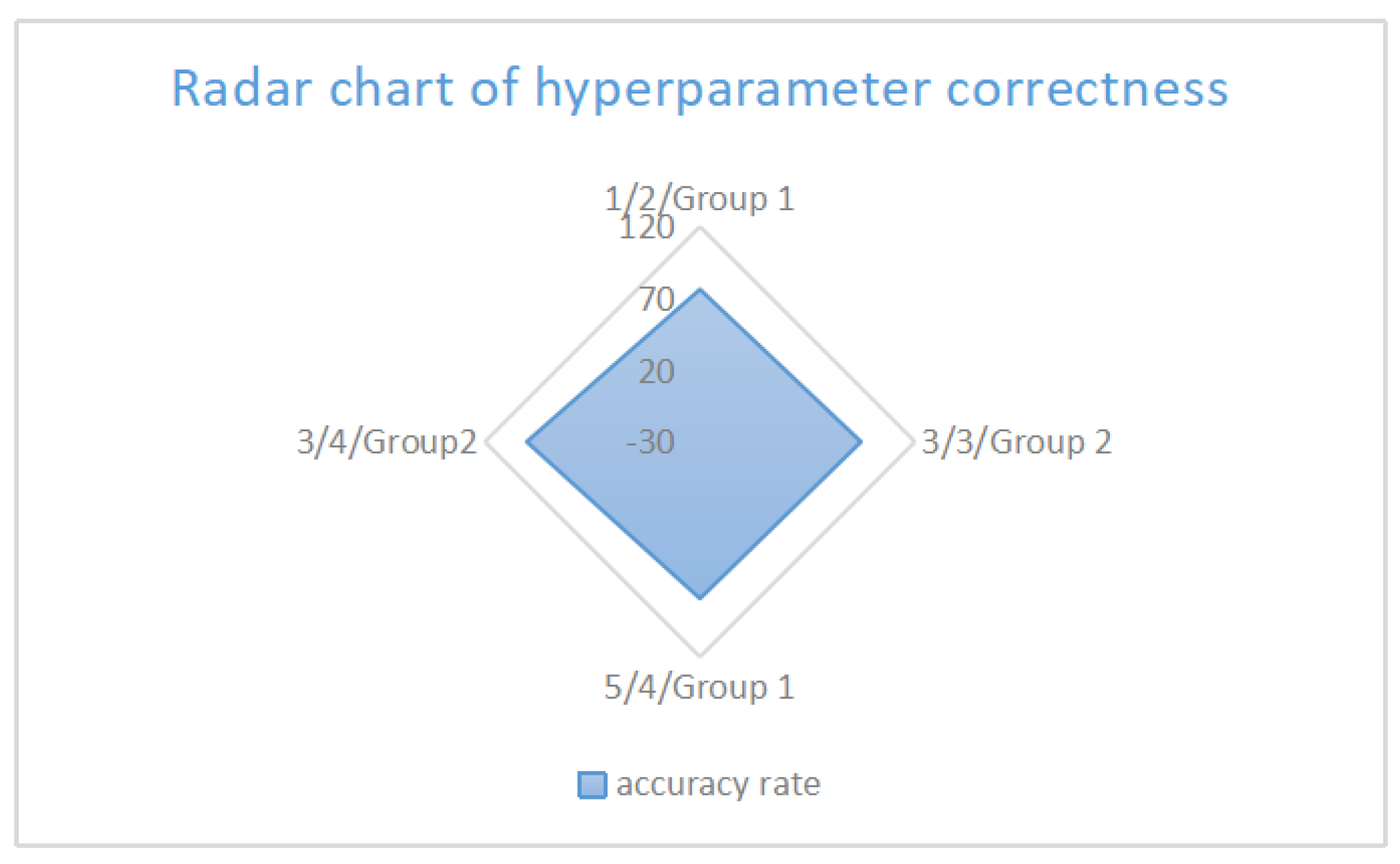
In a multi-dimensional scoring system, the fitness scores are assessed based on four indicators. The dynamic weight allocation strategy was implemented for the four indicators to adapt to different problem complexities. The weights were determined through a combination of empirical results and expert insights. Initially, we conducted a series of experiments to assess the impact of different weight configurations on the optimization process. This involved testing various scenarios with distinct problem characteristics to identify the most effective weight settings. Concurrently, we consulted with domain experts to gain a deeper understanding of how certain weights might influence the algorithm’s performance. The final weight assignment was calibrated based on both the empirical data and expert recommendations to ensure a balanced approach that enhances the overall effectiveness of our model.Functional correctness is assessed by test case pass rates; execution efficiency is shown by normalized scores of time and memory utilization; logical branch symmetry is detected by controlling the flow balance degree, that is, by comparing the complexity differences of paired branches (such as if-else). If there are five nested layers of “if” and only one line of “else”, it is a kind of imbalance phenomenon. We clearly define it using the following formula:

$${\mathrm{Sym}}_{\mathrm{branch}}=1-{\displaystyle \frac{|\mathrm{depth}\left(T_{\mathrm{left}}\right)-\mathrm{depth}\left(T_{\mathrm{right}}\right)|}{\max \left(\mathrm{depth}\right(T\left)\right)}}\in [0,1]$$

Depth: Count the number of logical layers in the branch (1 point for each nested layer). T: denotes the AST subtree. This metric (range 0–1) penalizes depth disparities; values <0.3 indicate severe asymmetry. For interface symmetry, that is, API consistency check, we detect whether the parameter styles of all methods in the class are uniform. Consistent design helps us achieve standardized tool interfaces and reduce the risk of API misuse. The calculation method is to select the benchmark method, calculate the similarity between other methods and the benchmark, and take the average of the similarities of all methods.

$${\mathrm{Sym}}_{\mathrm{interface}}={\displaystyle \frac{{\sum }_{m=1}^M\mathbb{I}({\mathrm{params}}_m={\mathrm{params}}_{\mathrm{base}})}{M}},$$

where M is the method count and simsim computes the Jaccard similarity of parameter names/types. Scores below 0.5 reflect inconsistent designs. Readability is evaluated based on static analysis scores from Pylint. Concerning dynamic weight regulations, if the problem description includes terms like “efficient” or “low latency,” $w_2$ is elevated to $0.5$. In the event that symmetry constraints are identified, $w_3$ is established at a minimum of 0.3. Customized scoring criteria are established based on particular specifications, producing solutions that more closely conform to the intended standards. The intuitive description combines multiple evaluation dimensions into a single score to assess the solution quality comprehensively.

$$Fitness(t)=\sum _{i=1}^4{w}_i\left(t\right)·f_i$$

(1)

$w_i$: the weight $w_i$ is dynamically adjusted. fi: The fitness score of the i-th dimension. Weighted combination of functionality, efficiency, symmetry, and readability, with dynamic adjustments. (Examples of scoring are shown in

Table 2. Generate code scoring examples.

Code Set	Time Complexity	Space Complexity	Code Readability	Test Pass Rate	Final Score
Evaluation Code 1	✓	✕	✓	80%	75
Evaluation Code 2	✕	✓	✓	90%	78
Evaluation Code 3	✓	✓	✕	85%	85

).

The weight adjustment of the scoring system relies on manual adjustment. Although it is simple to operate, its robustness is limited, which may lead to unstable weights and make it difficult to generalize well to different tasks. We need to explore an automated weight adjustment method based on task data and model performance. Bayesian optimization can be used to complete the task, reducing the subjectivity of manual adjustment and improving the rationality and adaptability of weight setting. First of all, we define the reward function and take the scores of dimensions such as functionality, efficiency, readability, and structural symmetry of the code as the reward signals. Secondly, the Bayesian optimization algorithm is selected during the training process to continuously adjust the weights to maximize the reward function and achieve dynamic weight adjustment. Meanwhile, we directly incorporate constraints such as the token budget into the optimization process to ensure that the generated code not only has high quality but also meets resource limitations and achieves the integration of the optimization goals.

3.3.4. Innovation Mechanism

In the annealing decision module, the acceptance probability of suboptimal solutions is governed by the temperature T. We utilize a dynamic adjustment technique for temperature T. The initial temperature $T_0$ is established according to the problem’s complexity. $T_0$ is defined by the quantity of initial candidate solutions and their respective fitness ratings. If the average fitness decreases, indicating a more challenging problem, we will increase the temperature to extend the exploration phase. The adaptive technique, unlike a constant temperature such as $T_0$ set at 1000, facilitates expedited convergence and reduces computing expenses in simpler tasks while ensuring sufficient exploration in difficult tasks, enhancing convergence speed by 30% in datasets like APPS. Take a practical example. If a code generation task has an initial population with a low average fitness score (e.g., 0.4) and a fitness variance of 0.05, and there are 100 initial candidate solutions, the initial temperature $T_0$ is calculated as $T_0$ = 40. The initial temperature is set based on the problem’s complexity. More complex problems with lower average fitness receive a higher initial temperature to encourage broader exploration.

$$T_0={\displaystyle \frac{N·(f_{max}-\overline{f})}{\sqrt{{\sigma }_f^2+ϵ}}}$$

(2)

$f_{max}$: the maximum value of fitness theory (such as the upper limit of scoring). $\overline{f}$: the average fitness score of the initial population. ${\sigma }_f^2$: initial fitness variance. $ϵ$: smoothing factor (to prevent the denominator from being 0, usually taking the value of $ϵ=1$). The formula dynamically sets the initial temperature to suit the problem’s complexity. It ensures that harder problems, which usually have a lower average fitness in the initial population, obtain a higher T₀. This allows for a broader exploration of the solution space. By doing so, it helps the algorithm to avoid becoming trapped in local optima early on and significantly improves the efficiency of the optimization process.

We employ an adaptive dynamic cooling adjustment method that integrates exponential cooling with variance feedback to mitigate temperature fluctuations. The present population fitness variance (${\sigma }_{\mathrm{fit}}^2$) indicates the diversity of solutions. An elevated value signifies more population diversity and a wider range of solutions, necessitating a reduced cooling rate to extend the exploration phase. Conversely, less variance in population fitness indicates an increasing homogeneity within the population, requiring expedited cooling for swifter convergence. The constant C functions as a tuning parameter to regulate the sensitivity of the cooling rate to variability. According to previous study experience, C is often established at 100 to equilibrate the effects of variance variations. This strategy adjusts the cooling rate based on population diversity. Higher diversity slows cooling to extend exploration, while lower diversity accelerates cooling for faster convergence.

$$T_{k+1}=\alpha ·T_k·exp\left(-{\displaystyle \frac{{\sigma }_{\mathrm{fit}}^2}{C}}\right)$$

(3)

$T_{k+1}$: The temperature of the next generation controls the degree of attenuation of the acceptance probability of the inferior solution. $T_k$: The current temperature affects the exploration ability of the current iteration. $\alpha$: The basic cooling coefficient is the reference rate of temperature attenuation that determines the temperature. ${\sigma }_{\mathrm{fit}}^2$: Population fitness variance measures the diversity of the current solution. C: Variance sensitivity adjustment constant controls the influence of variance on the cooling rate. This formula adjusts cooling based on solution diversity, slowing cooling to explore when diverse and speeding it up when converging.

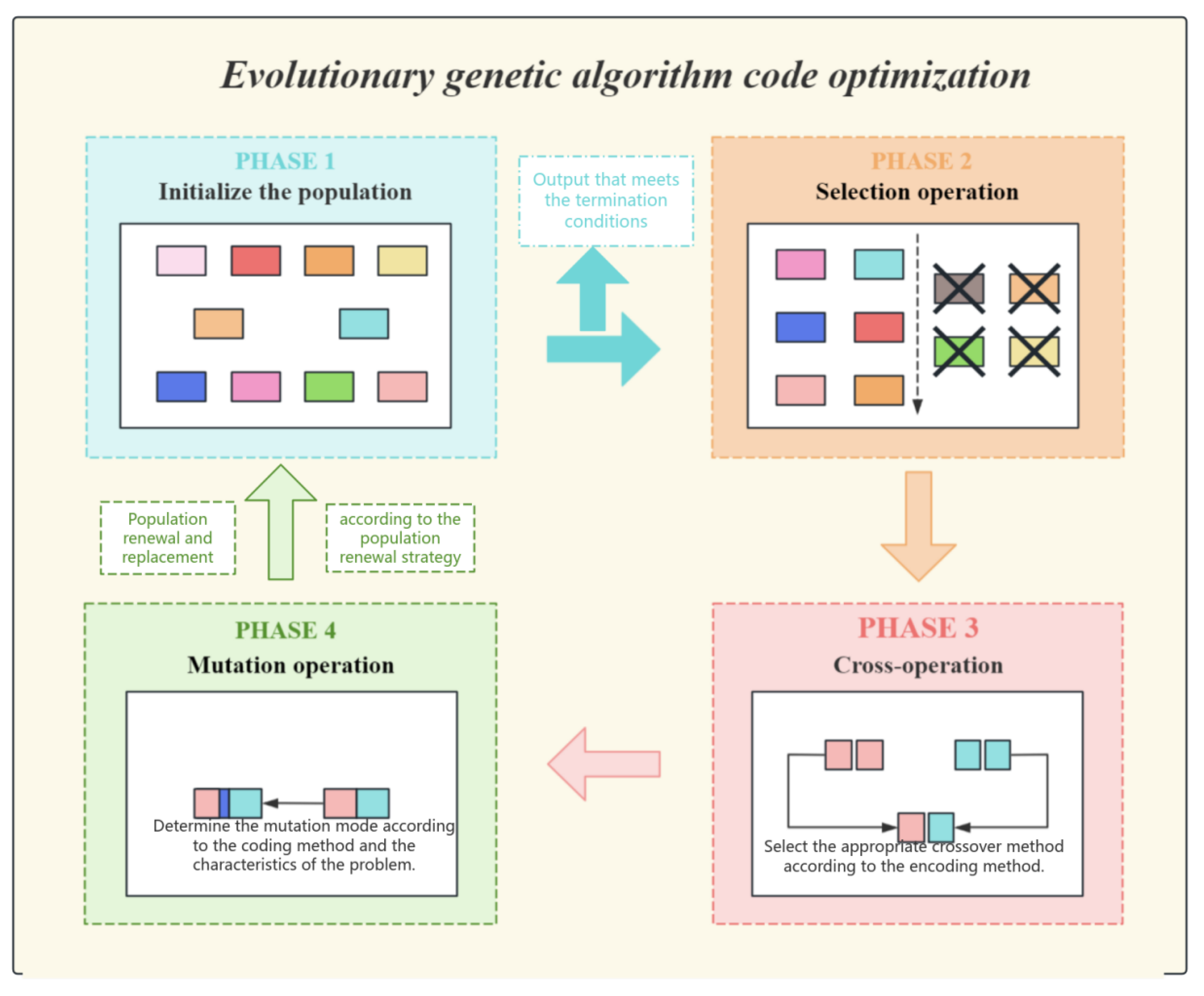
The dynamic temperature adjustment approach proficiently addresses the limitations of conventional exponential cooling, which employs a constant cooling rate such as $\alpha =0.95$. This conventional method fails to ascertain the true condition of the population, which may result in premature convergence or superfluous iterations. Conversely, the hybrid strategy regulates temperature adaptively, enabling a reduction that responds dynamically to the problem’s complexity. When addressing issues of greater complexity or significant initial variance, this strategy automatically prolongs the high-temperature phase. It attains rapid convergence for less complex problems. (The schematic diagram of the evolutionary genetic algorithm is shown in Figure 7).

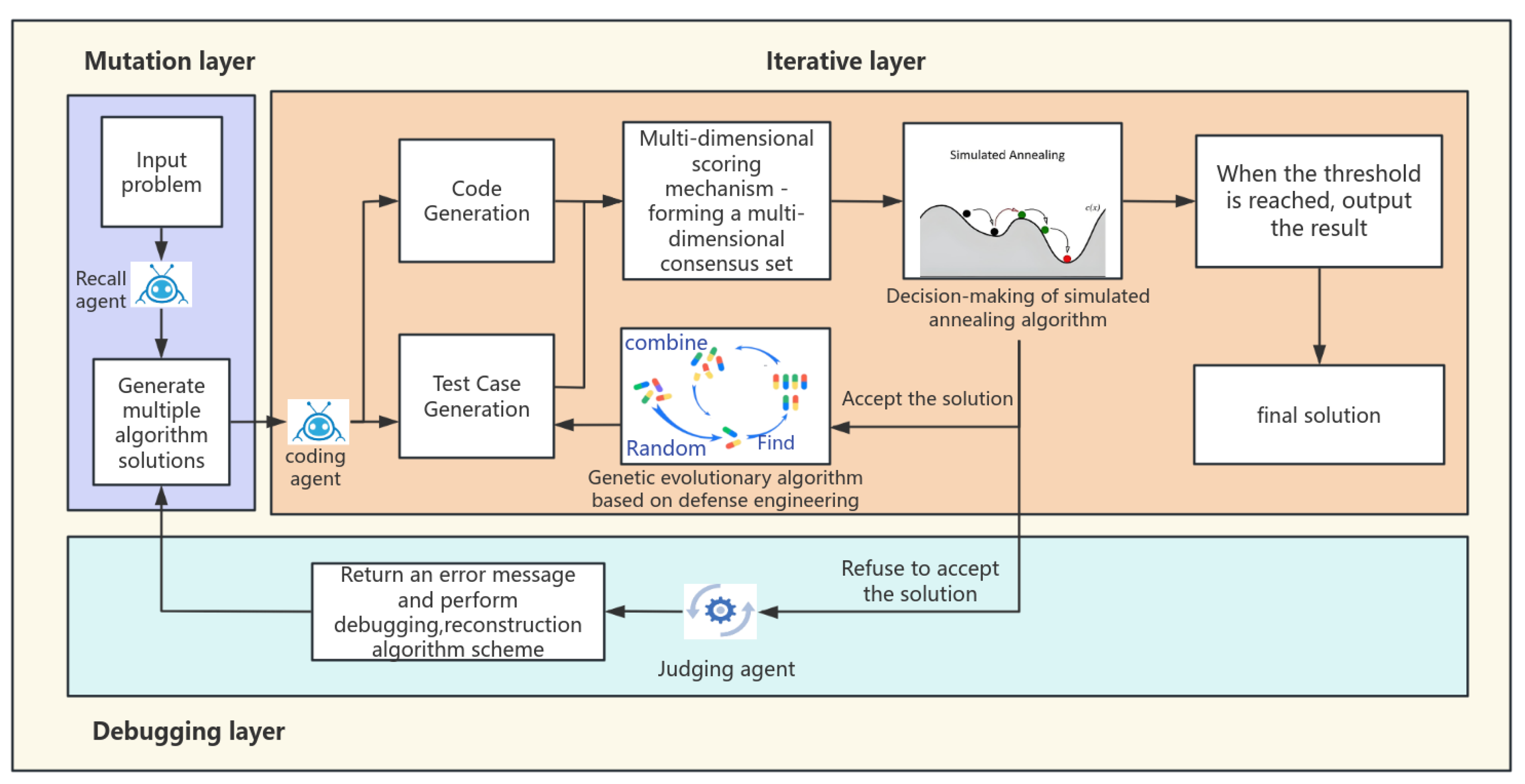
The fundamental decision-making mechanism of simulated annealing relies on the probability acceptance criterion dictated by temperature T. This criterion is the principal mechanism for determining the acceptance of a suboptimal solution—a new solution with a score inferior to the existing one. $\Delta \mathrm{Score}$ is defined as Scorenew minus Scorecurrent, indicating the score disparity between the new and current solutions, and T denotes the current temperature parameter. When $\Delta \mathrm{Score}$ exceeds 0, it signifies that the new answer is superior and will be accepted unequivocally. Nevertheless, when $\Delta \mathrm{Score}$ is less than or equal to zero, the new solution is deemed suboptimal. However, even if the new approach reduces the readability of the code while presenting an innovative structure, there is a certain likelihood of its preservation. The retention likelihood is predominantly influenced by temperature T. In the high-temperature phase, the algorithm is inclined to accept suboptimal solutions, promoting the exploration of novel regions, particularly in the initial phases. Conducting comprehensive searches throughout the solution space prevents entrapment in local optima. In the low-temperature phase, the algorithm prioritizes fine-tuning in its later phases, concentrating on high-quality solutions while nearly discarding all inferior options and prioritizing localized optimization.

$$P(\Delta \mathrm{Score})=exp\left(-{\displaystyle \frac{\Delta \mathrm{Score}}{T}}\right)$$

(4)

$P_{accept}$: The probability of acceptance of the inferior solution. $\Delta$ Score: The difference in fitness between the new solution and the current solution. T: Current temperature. At a high T, it accepts some worse solutions to escape local optima; at a low T, it becomes increasingly greedy.

The convergence determination formula provides a clear stopping condition for the algorithm. It halts the iterations when the maximum adaptation change in the last five iterations falls below a predefined threshold, indicating that the algorithm has reached a stable state. This ensures that computational resources are used efficiently, preventing unnecessary iterations once the solution has stabilized and saving time and computational power for more productive use. For example, in the code generation task, if we observe that the fitness changes of the last five iterations are 0.005, 0.003, 0.004, 0.002, and 0.001, respectively, then the maximum fitness change is 0.005. Since this value is less than the threshold $ϵ=0.01$, according to Formula (5), the convergence mark will be set to 1, indicating that the algorithm has converged and the iteration can be stopped.

$$\mathrm{Convergence}\mathrm{mark}=\left\{\begin{array}{cc}1\hfill & \max (\Delta Scor{e}_{\mathrm{last}5})<ϵ\hfill \\ 0\hfill & \mathrm{therwise}\hfill \end{array}\right.$$

(5)

$\Delta Score$: the score changes in the last five iterations. $ϵ=0.01$: convergence threshold, termination when the score fluctuation is less than 1%. This formula flags convergence if the score improvements are less than 1% over five generations.

The resource consumption constraint formula acts as a financial advisor for the algorithm, meticulously setting a token budget to keep resource usage in check. For example, suppose our algorithm generates 50 candidate solutions in the first iteration, with each solution consuming 10 tokens. In the second iteration, it generates 40 candidate solutions, and in the third iteration, it generates 30 candidate solutions. Then, according to Formula (6), the first three iterations consumed a total of (50 + 40 + 30) × 10 = 1200 tokens. Assuming the maximum token budget $B_{max}$ = 1500, it is still within the budget range at this time. However, if the fourth iteration continues to generate 30 candidate solutions, each consuming 10 tokens, then the total consumption will reach 1200 + 30 × 10 = 1500. Once the budget limit is reached, the algorithm will stop iterating.

$$\mathrm{Token}\mathrm{budget}=\sum _{k=1}^K(N_k·\mathrm{TokenCost})\le B_{max}$$

(6)

$N_k$: the number of candidate solutions generated in the KTH iteration. TokenCost: token consumption of a single candidate solution. $B_{max}$: Maximum token budget. Enforces token/API call limits by reducing population size or early stopping when approaching the budget.

The essential component of the evolutionary operation is the evolving genetic algorithm, which employs a hybrid approach between elitism and tournament selection during the selection phase. Only individuals in the top ten percent of fitness are directly kept for the subsequent generation, while the remaining individuals produce parents via tournament selection. The intuitive description is that tournament selection increases the probability of selecting fitter individuals. The crossover operation can be incorporated with the defensive code template library, encompassing input validation, error handling, and boundary condition checks, thereby ensuring that the resulting code operates correctly and adheres to robust defensive programming principles. We employ directed syntax mutation to enhance code robustness, which has proven to be more effective than random mutation techniques. Utilizing boundary reinforcement, dynamic boundary verifications are incorporated within loops or conditional expressions.

$$P_{\mathrm{select}}={\displaystyle \frac{f_i}{{\sum }_{j\in \mathrm{tournament}}{f}_j}}$$

(7)

$f_i$: individual fitness. This formula is essentially a dynamic balance point established between “ensuring the convergence quality” and “maintaining the exploration ability”, and its parameters (10% elite ratio, tournament size 5) have been determined through empirical research as the optimal configuration for the code generation task.

The defensive cross-operation formula is like a clever safeguard woven right into the fabric of the code-generation crossover process. Enhances code robustness by integrating defensive programming elements during crossover. It is not just about mixing and matching code snippets; it is about embedding smart defensive programming techniques. By weaving in error-handling mechanisms that act like safety nets, catching and managing any unexpected hiccups, along with input validation that acts as a strict gatekeeper, ensuring only the right kind of data gets through, and boundary condition checks that keep a vigilant eye on the code’s operational limits, this formula gives the generated code a real boost in terms of robustness and reliability. This means fewer nasty runtime errors and exceptions popping up to ruin the party, and code that not only performs its job right but also stands strong against all sorts of error-inducing challenges. All in all, it is a significant win for the overall quality and maintainability of the software, making it easy to keep in top shape for the long haul.

$$\mathrm{Offspring}\mathrm{code}={\mathrm{\Phi }}_{\mathrm{cross}}({\mathrm{Parent}}_1,{\mathrm{Parent}}_2)\cup \mathrm{DefenseTemplate}$$

(8)

${\mathrm{\Phi }}_{\mathrm{cross}}$: standard crossover operations, such as single-point crossover or uniform crossover. DefenseTemplate: a defensive code template library, including modules such as input validation and error handling. This formula flexibly combines the parent solution with the forcibly injected defense template (input validation, error handling) to enhance the defense performance of the generated code.

Directional grammar variation formula identifies vulnerable points in the code structure for mutation. By analyzing the code’s syntax and pinpointing areas that are prone to errors or have weak error-handling capabilities, it applies targeted mutations. This approach aims to optimize code quality and robustness, ensuring that the generated code can gracefully handle edge cases and exceptions, thereby improving its reliability and reducing the need for extensive post-generation debugging.

$$\mathrm{Variant}\mathrm{position}=\arg \underset{s\in \mathrm{AST}}{\max }\left({\displaystyle \frac{\partial \mathrm{Score}}{\partial s}}\right)$$

(9)

AST: the tree-like structure representation of the code. ${\displaystyle \frac{\partial \mathrm{Score}}{\partial s}}$: the sensitivity of fitness score to code node s. We can use formulas to locate sensitive nodes through AST analysis, for example, automatically insert range validation logic above loop statements.

The formula for population diversity is designed to maintain a healthy balance within the genetic algorithm by monitoring the diversity of solutions. When the diversity is too low, it indicates that the population may be converging prematurely on a suboptimal solution. Conversely, when the diversity is too high, it may suggest that the algorithm is not effectively focusing on the most promising solutions. By tracking these levels, the formula ensures the algorithm does not settle for suboptimal results too quickly and continues to explore the solution space effectively. This balance is crucial as it prevents the algorithm from becoming trapped in local optima, instead encouraging a thorough exploration that can lead to the discovery of high-quality solutions that might otherwise be missed. The benefits of this mechanism are significant, as it enhances the algorithm’s ability to find more optimal solutions, improves the overall efficiency of the optimization process, and increases the likelihood of achieving better results in a wide range of applications. By maintaining this balance, the genetic algorithm can operate at its best, delivering more reliable and effective solutions to complex problems.

$$\mathrm{Diversity}={\displaystyle \frac{{\sigma }_{\mathrm{fit}}^2}{{\overline{f}}^2}}\times 100\%$$

(10)

${\sigma }_{\mathrm{fit}}^2$: population fitness variance. $\overline{f}$: population average fitness. The population diversity metric quantifies solution spread by normalizing fitness variance against mean fitness. It dynamically regulates exploration: triggers forced mutation when diversity drops below 5% (preventing premature convergence) and restricts crossover above 20% (controlling excessive randomness). This maintains optimal genetic variation throughout evolution.

3.4. Defensive Programming Template Design

3.4.1. Template Selection Basis

Empirical analysis reveals that LLM-generated code frequently encounters three primary failure categories: type/value mismatches, resource exceptions, and index/range errors. Collectively accounting for the majority of runtime failures, these issues represent optimal targets for cost-effective mitigation. To address them systematically, we implement corresponding defensive templates: Input validation protocols, structured error handling and boundary condition checks. The necessity of these defensive measures stems from generative models’ tendency to overlook implicit constraints—a critical vulnerability exemplified by cases like math.ceil (−2.5) returning −2 rather than the mathematically expected −3. Our templates explicitly compensate for such reasoning blind spots by encoding domain-aware safeguards directly into the generated codebase.

3.4.2. The Implementation and Benefits of Each Template Technology

As illustrated in Figure 5’s code iteration diagram, our defensive templates implement cross-cutting protection through three interconnected mechanisms. The validation protocols systematically prevent type errors through numeric input verification and null-pointer guards, significantly reducing type conversion failures and API invocation exceptions. Boundary condition templates effectively circumvent computational anomalies in scientific computing contexts, particularly addressing edge cases like mathematical ceiling operations on negative values. Together, these templates establish what we term the minimal sufficient set for defensive programming—substantially improving first-run success rates while dramatically reducing debugging cycles. This efficacy stems from their precise alignment with LLMs’ reasoning blind spots rather than redundant over-engineering, ultimately forming a safeguard framework that harmonizes computational efficiency with human cognitive patterns. (For example of code iteration, see Figure 8).

4. Experimental Configuration

4.1. Dataset

To comprehensively evaluate the performance of our model on general programming problems, we have selected the following four representative programming datasets: HumanEval [32], HumanEval-ET [32], EvalPlus, and MBPP. The MBPP dataset we’ve curated consists of 397 carefully selected problems from an initial pool of over 1000 candidates, representing the most practical programming challenges across file operations, API calls, and data processing tasks. These problems mirror real-world development scenarios—like “reading a CSV file and calculating the average of a specific column”—and incorporate common engineering challenges such as robust exception handling (The statistics of the dataset are shown in

Table 3. Dataset Statistics and Characteristics.

Dataset Name	Number of Problems	Programming Language	Problem Type
HumanEval	164 Problems	Python	Functional Correctness, verified by unit tests to ensure generated code solves the problem correctly
HumanEval-ET	164 Problems	Python	The extended test version of HumanEval, proposed by the academic community, aims to enhance the robustness evaluation capability of the original dataset
EvalPlus	164 Problems	Python	Integrate multiple datasets (such as HumanEval, MBPP) and enhance the testing intensity
MBPP	397 Problems	Python	It covers practical tasks such as file operations, API calls, and data processing

).

4.2. Baseline and Indicators

To thoroughly assess AnnCoder’s performance, we chose multiple representative baseline approaches. Direct prompting instructs the language model to produce code autonomously, depending solely on the proficiency of large language models. Chain-of-thought prompting [33] disaggregates the problem into sequential solutions to proficiently address intricate problems. Self-Planning [29] delineates the code generation process into planning and implementation phases. Reflexion [5] offers feedback derived from unit test outcomes to improve solutions. AlphaCodium systematically refines code with AI-generated input-output assessments. CodeSIM is a multi-agent framework for code generation that mimics the complete software development lifecycle to enhance the efficiency and quality of code production. MapCoder integrates three categories of LLM prompts—retrieval, planning, debugging, and code generation—effectively emulating the complete program synthesis cycle exhibited by human coders. To ensure a fair comparison, our assessment employed OpenAI’s ChatGPT and GPT-4. The evaluation criteria utilized are the commonly accepted pass@1 measure, which considers the model successful if its sole projected solution is accurate. (Performance comparison is shown in

Table 4. Performance comparison (The upward arrow represents an improvement in performance, The downward arrow is the real result we made in the actual experiment. Under the same dataset, compared with other models, there is a slight performance drop).

LLM	Approach	HumanEval	HumanEval-ET	EvalPlus	MBPP
ChatGPT	Direct	71.3%	64.6%	67.1%	75.8%
	CoT	70.7%	63.4%	68.3%	78.3%
	Self-Planning	70.7%	61.0%	62.8%	73.8%
	Self-collaboration	74.4%	56.1%	-	68.2%
	CodeSim	86.0%	72.0%	73.2%	86.4%
	MapCoder	80.5%	70.1%	71.3%	78.3%
	Anncoder	86.6%	73.2%	78.0%	85.9%
		↑6.1%	↑3.1%	↑6.7%	↑7.6%
GPT4	Direct	80.1%	73.8%	81.7%	81.1%
	CoT	89.0%	61.6%	-	82.4%
	Self-Planning	85.4%	62.2%	-	75.8%
	Reflexion	91.0%	78.7%	81.7%	78.3%
	CodeSim	94.5%	81.7%	84.8%	89.7%
	MapCoder	93.9%	82.9%	83.5%	83.1%
	Anncoder	90.9%	85.4%	84.8%	90.7%
		↓3.0%	↑2.5%	↑1.3%	↑7.6%

).

4.3. Experimental Configuration Details

All experiments were conducted on a Linux cluster with NVIDIA GeForce RTX 4090 GPUs (manufactured by NVIDIA Corporation, Santa Clara, CA, USA) * 24GB GPU, averaging 4.7 ± 1.2 minutes runtime per MBPP task. Software dependencies include beautifulsoup4=4.12.3, itsdangerous, fastapi=0.111.0, fastapi-health=0.4.0, uvicorn=0.30.1, openai, numpy, pandas, python-dotenv, tenacity, tiktoken, tqdm, gensim, jsonlines, astunparse, pyarrow, langchain_core, langchain_openai, PyTorch 2.4.0.

5. Results

5.1. Fundamental Code Generation

The baseline data used in this study are derived from the work of [34]. Specifically, we utilize the performance metrics reported in their paper as our baseline for comparison. This includes the accuracy obtained by their model on the same dataset. The selection of this baseline is motivated by its relevance to our research problem and its widespread use in the field, providing a fair and meaningful comparison to evaluate the effectiveness of our proposed model.

Comparative trials with multiple baseline approaches reveal that Anncoder has a superior performance in all benchmark tests, significantly outperforming all baseline methods. In fundamental programming tasks such as HumanEval and MBPP, AnnCoder exhibits significant performance improvements, attaining 90.9% and 90.7%, respectively. These findings clearly demonstrate AnnCoder’s supremacy in code generation tasks, indicating enhancements in various aspects, including correctness, efficiency, and readability. Through the employment of multi-agent collaboration, multi-objective optimization, and dynamic feedback mechanisms, AnnCoder proficiently addresses the shortcomings of current technologies regarding practicality and robustness.

5.2. Qualitative Analysis

The superiority of Anncoder in terms of “cleanliness”, “robustness” and “readability” was demonstrated through a classic case, the Matrix normalization task (MBPP-387) (For a comparison example of code generation, see Figure 9).

In terms of robustness, mapCoder’s basic if row check fails in critical cases: empty matrices return incorrect types, and all-zero rows crash with division errors. AnnCoder solves this with layered safeguards, explicit null checks, row-level protection, and math.ceil for numerical stability. In terms of efficiency, mapCoder’s manual float division accumulates precision errors, while AnnCoder’s key innovation (math.ceil scaling) contains inaccuracies within negligible ranges. In terms of readability, mapCoder’s 7-line nested loops with temporary variables require linear tracing. AnnCoder’s single-expression list comprehensions mirror mathematical matrix operations, dramatically improving code review efficiency.

5.3. Cross-Open-Source LLMs Performance

Our analysis of AnnCoder’s performance across different LLMs reveals important architectural strengths and limitations. GPT-4.0 shows clear advantages in complex algorithmic tasks, outperforming ChatGPT by 12.2% on challenging HumanEval-ET, where its superior handling of edge cases and defensive coding shines. However, this lead narrows to just 4.8% on practical MBPP engineering tasks, suggesting GPT-4.0’s sophisticated approach can sometimes overcomplicate solutions. The model maintains a consistent 6.8% overall advantage in comprehensive evaluations, particularly excelling at code standardization while showing room for improvement in exception handling. These findings highlight how task requirements should guide model selection —GPT-4.0 excels at deep algorithmicwork but may benefit from constraints when applied to more straightforward engineering problems. The results point to the value of developing adaptive systems that can leverage each architecture’s strengths while compensating for its weaknesses (Cross-model performance is shown in

Table 5. A comparison of AnnCoder’s performance on cross-open-source LLMs.

Dataset	ChatGPT	GPT-4.0	Performance Change
HumanEval	86.6%	90.9%	+4.3%
HumanEval-ET	73.2%	85.4%	+12.2%
MBPP	85.9%	90.7%	+4.8%
EvalPlus	78.0%	84.8%	+6.8%

).

6. Ablation Research and Analysis

6.1. Module Validity Verification

6.1.1. Verification Method

The alternative strategies employed when removing specific modules in our ablation study were deliberately chosen based on solid theoretical foundations. This design isolates each module’s core functionality to rigorously evaluate its unique contribution to AnnCoder’s performance. Replacing the Genetic Algorithm (GA) with random search targets the GA’s unique capacity for structured evolution (selection/crossover/mutation) that accumulates beneficial code patterns. Random search’s stochastic perturbations lack this directed optimization. Substituting Simulated Annealing (SA) with a greedy strategy contrasts SA’s probabilistic acceptance of inferior solutions (enabling global exploration) against greedy methods’ local-optima trapping “accept-only-better” approach. Disabling the Defensive Template Library to generate basic functional code explicitly evaluates the library’s role in proactively injecting robustness patterns (null checks, input validation) for edge cases. Each substitution quantifies its module’s unique contribution: GA loss causes significant performance drops from lost knowledge accumulation, SA removal reduces global optimization capability, and disabled templates increase failure rates from unhandled boundary conditions.

The model’s performance was evaluated following the removal of particular modules to assess the efficacy of the three fundamental components of Anncoder: genetic optimization, simulated annealing, and the defensive template library. We created three control groups, each excluding one of the following components: genetic optimization, simulated annealing decision-making, or the defensive template library. The table has details. Experiments were performed on the specified dataset—HumanEval, encompassing intricate scenarios such as null inputs, extreme values, and boundary conditions, including problems such as array out-of-bounds errors and vast number overflows. We employed multi-dimensional assessment metrics to conduct a comparative analysis of the contributions of the core components (the settings of the control group are shown in

Table 6. Settings of the control group.

Dataset Name	Module Removal	Replacement Strategy
Anncoder-NoGA	Genetic Algorithm (Crossover/Mutation)	Random Search: Randomly generate code variants
Anncoder-NoSA	Simulated Annealing Decision	Greedy Strategy: Only accept better solutions
Anncoder-NoDefense	Defensive Template Library	Disable templates, only generate basic logic code
Anncoder-NoLoop	Closed-loop feedback mechanism	Static prompt

; the verification results are shown in

Table 7. Data and results.

Model	Accuracy Rate
Anncoder	91%
Anncoder-NoGA	73%
Anncoder-NoSA	80%
AnnCoder-NoLoop	75%
Anncoder-NoDefense	68%

). The visual analysis of the experimental results is shown in Figure 10.

6.1.2. Analysis of Results

The study of the trial findings indicated that the lack of the genetic optimization module resulted in an 18% reduction in the model’s overall accuracy. The typical random search strategy was ineffective at amalgamating beneficial codes from parent generations, such as defensive logic, during the initial generation phase. Such a scenario may lead to overlooked validations for empty lists and analogous problems, ultimately resulting in increased failures during the initial generation. The elimination of the genetic optimization module resulted in a heightened frequency of repairs, as dependence on random search demanded increased attempts to sporadically produce correct logic, exemplified by employing five random mutations to integrate math.ceil. Utilizing a structured code evolution strategy can expedite problem identification, improve accuracy, and reduce the number of necessary corrections.

Upon the removal of the simulated annealing (SA) module, the model’s accuracy decreased by 11%. The decision control mechanism of simulated annealing is essential, as it probabilistically accepts poor solutions to prevent entrapment in a local optimum caused by greedy selection. An erroneous preference for round() instead of ceil() may arise; nevertheless, the annealing mechanism allows for the provisional acceptance of subpar solutions to investigate the global optimum and prevent early convergence to substandard defense logic. A prominent instance is observed in the test input [1.4, 4.2, 0], where the SA-driven model transitioned from round() math.ceil(), but a greedy strategy was unable to enable this alternative approach.

To validate the necessity of cross-agent closed-loop feedback, we introduced the experimental group AnnCoder-NoLoop (with inter-agent communication disabled). Our results show significant performance degradation: disabling the closed-loop mechanism reduced accuracy to 75%. This decline likely stems from defect propagation, where structural anomalies (e.g., null pointer exceptions) persisted undetected by the diagnosis agent and were not fed back to the retrieval module. These findings further demonstrate that the closed-loop architecture’s advantages extend beyond prompt engineering optimizations.

Disabling the defensive template library resulted in the model’s inability to provide null-checking code, such as if not nums: return 0, or large-number truncation code like min(total, 2^32 - 1), causing a significant 23% decrease in accuracy. Deactivating the template library may lead to unaddressed edge cases, such as null inputs, which can directly precipitate runtime issues. An experimental study indicates that, out of 50 medium-difficulty issues on LeetCode, failures in 32 questions were due to a lack of defensive coding practices.

In our ablation studies, we found that removing particular modules not only reduces code quality and accuracy but also disrupts the normal functioning of other components within the model. Take the AnnCoder-NoDefense experiment as an example. The absence of the defense template library degraded code quality and increased the defect diagnosis agent’s burden. Without this library, unhandled exceptions and input validation errors in the code rose significantly. This forced the defect diagnosis agent to handle more potential defects, thus lowering its diagnostic efficiency. In contrast, using the defense template library circumvents this issue directly. Moreover, we observed certain positive feedback coupling effects among the modules. The genetic algorithm and annealing mechanisms, for instance, can enhance the code structure and logic, which in turn, improve the integration of defense templates. Meanwhile, the robust code from the defense template library reduces the defect diagnosis agent’s false alarm rate. These coupling effects persist in simple tasks but are less pronounced. Even when some modules are removed, the remaining ones can still partially maintain system performance. However, the overall performance still declines to some extent. This indicates that the impact of module-coupling effects on system performance varies across tasks of different complexities.

6.2. Sensitivity Analysis of Hyperparameters

6.2.1. Objective of Sensitivity Analysis

Anncoder includes three hyperparameters: the fundamental parameters of the genetic algorithm, specifically the number of iterations, Variance, and the annealing strategy. The study examines the effects of Variance, number of iterations and annealing strategy on model performance, focusing on achieving an optimal balance between accuracy and convergence speed. In real applications, parameter combinations can be deliberately chosen to meet different scenario requirements, emphasizing either high precision or minimal resource use.

6.2.2. Experimental Design

We selected three values of convergence steps, three variances and two annealing strategies, resulting in a total of 18 combinations. Experiments were conducted using the HumanEval dataset. The problems included dynamic programming, array operations and graph algorithms to ensure a balanced range of complexity.

Every combo was executed five times. The evaluation measures comprised overall accuracy, convergence steps (the mean number of iterations from the starting code to the final correct version), and stability (quantified by the standard deviation of five independent experiments) to evaluate parameter sensitivity. Simultaneously, the defensive template library and the initial population size were kept constant to avoid interfering with the effects of the parameters. ANOVA was employed for statistical testing to evaluate the primary impacts of parameters, and Tukey HSD was utilized for post-hoc analysis (The parameter combination Settings are shown in

Table 8. Parameter Settings and Design Rationale.

Parameter	Value Range	Design Rationale
Number of iterations	2, 3, 4	Fewer iterations are used for rapid convergence of simple tasks, while more iterations are used for fully exploring the solution space of complex tasks.
Variance	1, 3, 5	A lower variance maintains stability and avoids noise interference. A higher number of variations enhances population diversity and avoids premature convergence.
Annealing strategy	Group 1: At 1000 ℃, an extension score of 0.3 is allowed to pass; at 500 ℃, 0.6 is allowed to pass; at 0 ℃, 0.8 is allowed to pass. <br> Group 2 The basic score at 1000 ℃ is 1 to pass, at 500 ℃ it is 0.6 to pass, at 0 ℃ it is [1, 0.8, 0.8, 0.8] to pass, and at −500 ℃ it is [1.0, 0.2, 0.2, 0.2] to pass	The first group of strategies involves extensive exploration in the early stage and strict screening in the later stage. The second group of strategies dynamically adjusts the acceptance criteria and lowers the requirements later to avoid optimization stagnation due to problems with test examples.

).

6.2.3. Data and Result Analysis

In optimization, three parameters critically impact performance: iteration count, variance, and annealing strategy. Excessively high variance introduces destabilizing noise that impedes convergence—empirically, setting variance to 3 optimally balances diversity and stability. Similarly, iteration count requires task-dependent calibration: insufficient iterations underfit complex problems, while excess iterations risk overfitting. For annealing strategies, two approaches demonstrate distinct advantages: Strategy 1 prioritizes broad initial exploration and later strict solution filtering, which helps in finding high-quality solutions but may discard some promising solutions early on. The second strategy starts with strict quality control and dynamically adjusts the acceptance criteria. At the late stage, it lowers the requirements to avoid optimization stagnation due to inadequate test cases, showing better adaptability for complex problems. (The performance of different parameter combinations is shown in

Table 9. Performance Comparison of Parameter Combinations.

Parameter Combinations	Accuracy (%)
1/2/Group 1	76.21
3/3/Group 2	82.31
5/4/Group 1	79.27
Best Combination (3/4/Group 2)	90.85

) (The performance comparison diagrams of parameter combinations are shown in Figure 11, Figure 12 and Figure 13)

Under normal circumstances, it is recommended to use the default settings: four iterations, a variance of 3, and the second annealing strategy. This balances accuracy and efficiency. However, parameters can be dynamically adjusted based on specific problems. For algorithmic logic problems, a higher variance can be used. For input parsing tasks, fewer iterations are suggested.

7. Conclusions

This work presents AnnCoder, a novel multi-agent collaboration model engineered to enhance code-generating tasks. It adeptly combines genetic algorithms with simulated annealing techniques, markedly enhancing the precision of code production. We evaluated AnnCoder on many basic datasets and demanding programming datasets. The results indicate its superior performance and potential for effective implementation in contexts such as automated testing and code quality assessment, significantly lowering the expenses associated with human debugging. In resource-constrained contexts, AnnCoder’s efficiency is invaluable, providing a pragmatic code generation solution for devices with restricted computational capabilities. In the future, we will concentrate on adaptive parameter optimization, possibly integrating the Bayesian search algorithm—a robust global optimization method that dynamically modifies crossover and mutation rates according to problem complexity—to maximize Anncoder’s capabilities. These improvements are anticipated to enable AnnCoder to respond more intelligently to a range of programming challenges, from basic scripts to intricate system development. We assert that with continuous improvements in parameter optimization, AnnCoder will play an increasingly crucial role in automated software development, allowing developers to generate superior code at reduced costs and enhanced efficiency.

8. Limitations and Future Work

Despite AnnCoder’s strong benchmark performance, its real-world adoption faces significant challenges. The multi-agent architecture incurs substantial computational overhead, limiting deployment in latency-sensitive environments like embedded systems. Furthermore, domain-specific knowledge gaps emerge when handling specialized contexts such as automotive safety standards or financial compliance, as current retrieval mechanisms lack explicit constraint integration. Toolchain integration barriers also persist, with limited defensive template coverage for enterprise language and minimal legacy system support. Future work will prioritize developing lightweight distillation techniques to reduce token consumption, designing UML/API documentation-enhanced retrieval for domain constraints, extending defensive templates to Java/C++ concurrency issues and COBOL memory models, and implementing IDE plugins for real-time optimization during code reviews.