Adaptive Control of Nonlinear Non-Minimum Phase Systems Using Actor–Critic Reinforcement Learning

Abstract

This study introduces a novel control strategy tailored to nonlinear systems with non-minimum phase (NMP) characteristics. The framework leverages reinforcement learning within a cascade control architecture that integrates an Actor–Critic structure. Controlling NMP systems poses significant challenges due to the inherent instability of their internal dynamics, which hinders effective output tracking. To address this, the system is reformulated using the Byrnes–Isidori normal form, allowing the decoupling of the input–output pathway from the internal system behavior. The proposed control architecture consists of two nested loops: an inner loop that applies input–output feedback linearization to ensure accurate tracking performance, and an outer loop that constructs reference signals to stabilize the internal dynamics. A key innovation in this design lies in the incorporation of symmetry principles observed in both system behavior and control objectives. By identifying and utilizing these symmetrical structures, the learning algorithm can be guided toward more efficient and generalized policy solutions, enhancing robustness. Rather than relying on classical static optimization techniques, the method employs a learning-based strategy inspired by previous gradient-based approaches. In this setup, the Actor—modeled as a multilayer perceptron (MLP)—learns a time-varying control policy for generating intermediate reference signals, while the Critic evaluates the policy’s performance using Temporal Difference (TD) learning. The proposed methodology is validated through simulations on the well-known Inverted Pendulum system. The results demonstrate significant improvements in tracking accuracy, smoother control signals, and enhanced internal stability compared to conventional methods. These findings highlight the potential of Actor–Critic reinforcement learning, especially when symmetry is exploited, to enable intelligent and adaptive control of complex nonlinear systems.

1. Introduction

The control of nonlinear systems with non-minimum phase (NMP) behavior remains a fundamental and long-standing challenge in the field of control engineering. These systems are particularly difficult to handle due to the presence of unstable internal zeros, which hinder precise output tracking and jeopardize the stability of internal states. This issue has attracted significant research attention and led to the development of numerous control strategies.

For example, Jouili et al. [1] proposed an adaptive control approach for DC–DC converters under constant power load conditions, emphasizing the challenge of achieving both output regulation and internal stability. Cecconi et al. [2] analyzed benchmark output regulation problems in NMP systems and identified the limitations of conventional methods. In the context of fault-tolerant control, Elkhatem et al. [3] addressed robustness concerns in aircraft longitudinal dynamics with NMP characteristics. Sun et al. [4] introduced a model-assisted active disturbance rejection scheme, and Cannon et al. [5] presented dynamic compensation techniques for nonlinear SISO systems exhibiting non-minimum phase behavior.

Alongside these contributions, various classical approaches have also been developed to address NMP-related difficulties. Isidori [6] introduced the concept of stable inversion for nonlinear systems, which was later extended by Hu [7] to handle trajectory tracking in NMP configurations. Khalil [8] proposed approximation methods based on minimum-phase behavior, while Naiborhu [9] developed a direct gradient descent technique for stabilizing nonlinear systems. Although these strategies provide valuable insights, they often offer only local or approximate solutions and may be less effective in highly nonlinear or uncertain environments.

Other significant efforts include the approximate input–output linearization using spline functions introduced by Bortoff [10], the continuous-time nonlinear model predictive control investigated by Soroush and Kravaris [11], and the hybrid strategies combining backstepping and linearization for NMP converter control developed by Villarroel et al. [12,13].

Within this framework, Jouili and Benhadj Braiek [14] proposed a cascaded design composed of an inner loop for input–output linearization and an outer loop using a gradient descent algorithm to stabilize the internal dynamics. Their stability analysis, based on singular perturbation theory, could potentially be reinforced by identifying and leveraging symmetric properties inherent in system dynamics.

Nevertheless, the reliance on gradient-based optimization presents notable shortcomings, especially in uncertain or highly variable environments. These limitations underscore the need for more intelligent and adaptive solutions, where recognizing symmetrical patterns in control structures and system behavior may offer enhanced generalization and robustness.

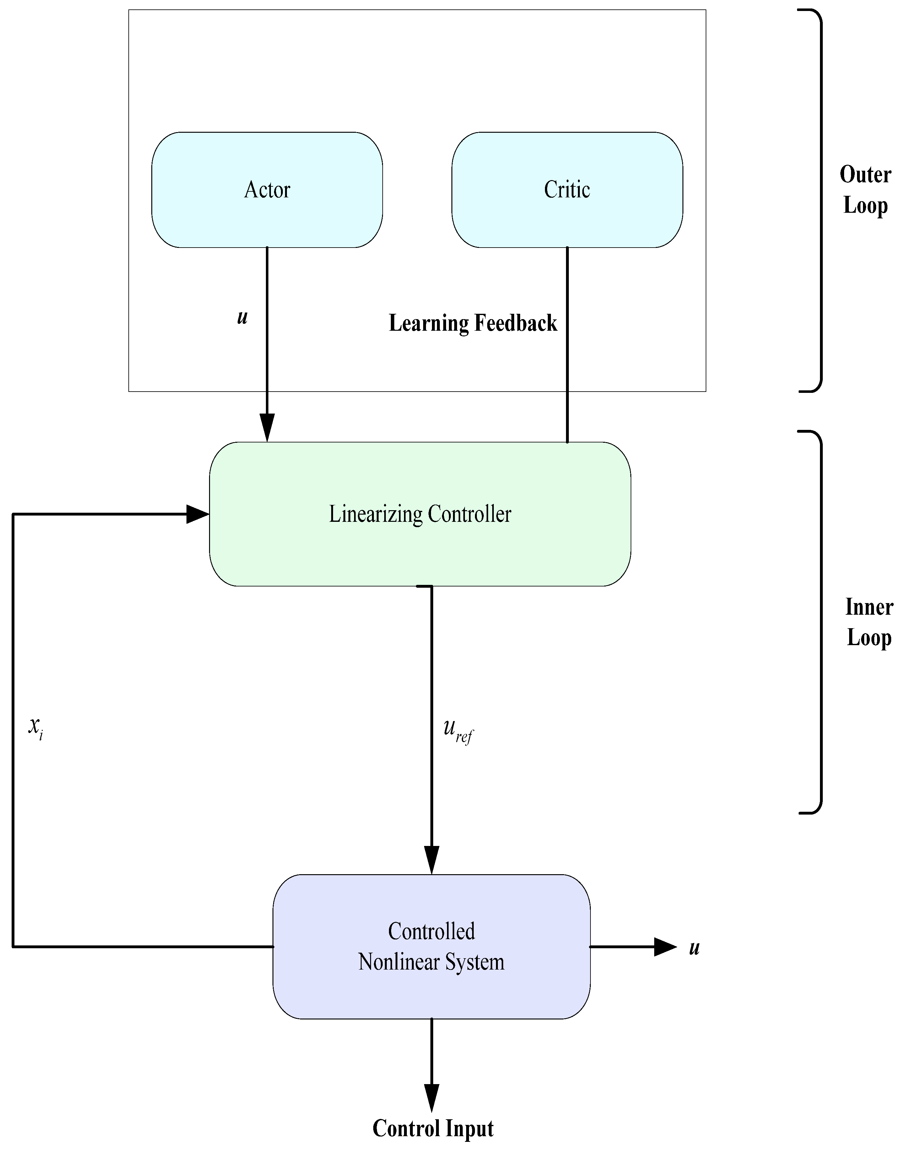
Our contribution lies in this direction: this article presents an innovative reformulation of the framework by Jouili and Benhadj Braiek [14], integrating a Reinforcement Learning (RL) approach, specifically through an Actor–Critic agent [15,16], to improve stability, robustness, and output tracking accuracy. The Actor–Critic approach allows an intelligent agent to learn an optimal control policy through continuous interaction with the system, guided by a reward function based on tracking accuracy and internal state stability. The Actor generates control actions, while the Critic evaluates the quality of these actions through value function estimates.

The resulting control scheme still relies on a cascaded architecture, where the inner loop is ensured by input–output linearization, and the outer loop is driven by the RL agent. The RL agent replaces the gradient descent controller with an adaptive and optimized policy during interaction. The stability analysis of the entire system is established using singular perturbation theory [8].

The proposed approach is evaluated through a case study involving an inverted pendulum on a cart, enabling a comparison of performance regarding tracking accuracy, stability, and transient response.

This article is organized as follows. Section 2 describes the architecture of the proposed control scheme. Section 3 covers the mathematical modeling of the system, while Section 4 discusses reinforcement-learning-based control. Section 5 presents the stability analysis of the control scheme, followed by the simulation results in Section 6. Finally, Section 7 concludes the article and suggests future research directions.

2. Proposed Control Scheme Architecture

2.1. A Gradient Descent Control Scheme

The control architecture introduced by Jouili and Benhadj Braiek [14] is based on a cascade structure aimed at managing the complexity of nonlinear, non-minimum phase systems in a hierarchical manner. This structure consists of two separate yet complementary control loops.

The inner loop focuses on input–output linearization. It uses the Byrnes–Isidori normal form, which separates the system’s dynamics into a directly observable part at the output and an unobservable internal part related to the non-minimum phase zeros. A linearizing controller is applied to convert the system into an equivalent linear model at the input–output level, ensuring precise trajectory tracking while simplifying the system’s observable dynamics.

The outer loop, in contrast, addresses the stabilization of the often unstable internal dynamics. In the classical setup, this stabilization is achieved through a gradient-descent-based controller, which generates a reference trajectory to guide the internal states toward stable behavior. The principle behind this method involves separating time scales by introducing a parameter ε, which differentiates the fast dynamics handled by the inner loop from the slower dynamics managed by the outer loop. This setup enables the application of singular perturbation theory for global stability analysis.

However, despite its theoretical rigor, this approach faces limitations in uncertain environments or when there are changes in the system dynamics. Specifically, the gradient descent controller requires precise parameter tuning and cannot adapt automatically to varying conditions.

2.2. Integration of the Actor–Critic Agent

To address these limitations, we propose replacing the gradient descent controller in the outer loop with a reinforcement-learning-based Actor–Critic agent. This adaptation allows the control scheme to dynamically optimize and adjust based on direct interactions between the agent and the system being controlled.

In this revised setup:

• The Actor generates the control actions based on the observed or estimated internal state of the system.
• The Critic evaluates the actions in real time, estimating their effectiveness through a reward function that considers both the stability of the internal dynamics and the accuracy of output tracking.

The learning process is iterative: after each cycle, the Critic updates its value function using a Temporal Difference (TD) learning method, while the Actor refines its policy to maximize future rewards. This approach enables the agent to converge toward an optimal control strategy without requiring explicit knowledge of the system’s dynamic model.

The resulting control scheme preserves the cascade structure: the inner loop continues to linearize the input–output dynamics, while the outer loop is enhanced by an autonomous learning process capable of adapting to and stabilizing the internal states as the system evolves. This hybrid combination of classical control techniques and artificial intelligence leads to a more robust, adaptable, and potentially higher-performing control system for complex real-world applications.

Figure 1 presents the architecture of a cascade control scheme incorporating a reinforcement learning agent based on the Actor–Critic model, where the secondary controller refines the agent’s actions to ensure optimal system performance.

3. Modeling of the System

3.1. Byrnes–Isidori Normal Form

Consider a Single-Input Single-Output (SISO) nonlinear system described by

$$\dot{x}=f\left(x\right)+g\left(x\right)u, y=h\left(x\right)$$

(1)

where $x\in {\Re }^n, u\in \Re$ and $y\in \Re$ and $f, g$ and $h$ are smooth functions (C^∞).

Assuming the system has a constant relative degree r < n and that the Lie derivative condition is satisfied:

$$L_g{L}_f^{\left(r-1\right)}h\left(x\right)\ne 0$$

(2)

We can apply a coordinate transformation to bring the system into the Byrnes–Isidori normal form. The new coordinates are defined as

$$z_1=h\left(x\right),z_2={\displaystyle \frac{d}{dt}}h\left(x\right),\dots , z_r={\displaystyle \frac{d^{\left(r-1\right)}}{{dt}^{\left(r-1\right)}}}h\left(x\right), \eta =\Phi \left(x\right)$$

(3)

where Φ (x) represents the internal dynamics (zero dynamics), and η $\in$ R^n−r.

The transformed system is given by

$${\dot{z}}_1=z_2, {\dot{z}}_2=z_3, \dots , {\dot{z}}_r=a\left(z, \eta \right)+b\left(z, \eta \right)u, \dot{\eta }=q\left(z, \eta \right), y=z_1$$

(4)

Here, z = (z₁, …, z_r) represents the linearized input–output dynamics, and η corresponds to the internal dynamics, which are typically non-minimum-phase and may be unstable.

The control law for feedback linearization is defined as

$$u={\displaystyle \frac{1}{b\left(z, \eta \right)}}\left[-a\left(z, \eta \right)+v\right]$$

(5)

Which results in the linearized input–output dynamics:

$${\dot{z}}_1=z_2, {\dot{z}}_2=z_3, \dots , {\dot{z}}_r=v$$

(6)

where v is a virtual input. However, the internal dynamics,

$$\dot{\eta }=q\left(z, \eta \right),$$

(7)

remain nonlinear and are not directly influenced by the control input u. Their stability is crucial for the overall system performance and must be treated separately.

3.2. Two-Time-Scale Formulation

To decouple the fast input–output dynamics from the slower internal dynamics, a two-time-scale representation is introduced using singular perturbation theory. A cascade control scheme is adopted as follows:

The inner loop performs the input–output linearization and forces the output z₁ to follow a desired reference trajectory $z_1^d$.

The outer loop generates the reference trajectory $z_1^d$, aiming to stabilize the internal dynamics η.

The complete control input is expressed as

$$u={\displaystyle \frac{1}{b\left(z, \eta \right)}}\left[-a\left(z, \eta \right)+{\ddot{z}}_d+{\displaystyle \sum _{i=1}^{r-1}{k}_i{\epsilon }_{i-1}{e}^{\left(i-1\right)}}\right]$$

(8)

where

$$e=z_1-z_1^d$$

(9)

is the output tracking error, ϵ ≪ 1 is a small positive parameter separating the time scales, and k_i represents the feedback gains designed to ensure rapid convergence of the output dynamics.

In the original work [14], the reference trajectory z_d is generated by a gradient descent law minimizing a cost function:

$$J\left(\eta , z_d\right)={\displaystyle \frac{1}{2}}{‖\eta ‖}^2$$

(10)

with:

$${\dot{z}}_d=-\epsilon {\displaystyle \frac{\partial J}{\partial z_d}}$$

(11)

This formulation leads to a slow evolution of z_d aimed at stabilizing η, while z tracks z_d rapidly. By introducing the fast-time variable $\tau ={\displaystyle \frac{t}{\epsilon }}$, the full system dynamics can be rewritten as

$$\left\{\begin{array}{l}\epsilon \dot{z}=f_1\left(z_1,\eta ,z_d\right)\\ \dot{\eta }=f_2\left(z_1,\eta \right)\\ {\dot{z}}_d=-\epsilon {\displaystyle \frac{\partial J}{\partial z_d}}\end{array}\right.$$

(12)

This is a singularly perturbed system, where z $\in$ R^r evolves on a fast-time scale, η $\in$ R^n−r evolves on a slow-time scale.

According to classical results from singular perturbation theory [8], if:

The fast subsystem (z→z_d) is asymptotically stable for fixed η,

The slow subsystem (η) is stable, when z = z_d, then the complete closed-loop system is asymptotically stable for sufficiently small ϵ.

In the next sections, we propose replacing the gradient descent mechanism with a reinforcement-learning-based agent, specifically using an Actor–Critic architecture, to generate z_d in a more adaptive and intelligent manner.

4. Reinforcement-Learning-Based Control

To overcome the inherent limitations of the gradient descent method used in the outer loop of classical control architectures, we propose replacing it with an RL strategy, specifically using an Actor–Critic framework. This structure enables an intelligent agent to dynamically generate the reference trajectory z_d based on the system’s current state, while simultaneously learning to maximize a reward associated with stability and tracking performance. The following control structure is proposed (Figure 2):

4.1. Actor–Critic Agent Structure

The Actor–Critic agent is composed of two main components:

• The Actor, which suggests an action a_t, i.e., an update to the reference trajectory z_d, based on the observed state s_t;
• The Critic, which evaluates this action by estimating the value function V(s_t) or the advantage function A(s_t, a_t), using the cumulative reward signal.

In our framework, the Actor generates an indirect control input that adjusts the desired output trajectory. Rather than relying on gradient descent:

$${\dot{z}}_d=-\epsilon {\displaystyle \frac{\partial J\left(\eta \right)}{\partial z_d}}$$

(13)

As used in traditional optimization, we adopt a policy-based update defined by:

$${\dot{z}}_d={\pi }_{\theta }\left(s_t\right)$$

(14)

where ${\pi }_{\theta }$ is the learned policy parameterized by neural network weights θ, and the state s_t = (η(t), z(t)) encapsulates the relevant system dynamics.

The Critic, on the other hand, estimates the expected return using the value function:

$$V_w\left(s_t\right)\approx {\rm E}\left[{\displaystyle \sum _{k=0}^{\infty }{\gamma }^k{r}_{t+k}/s_t}\right]$$

(15)

With the following notations:

ω: parameters of the Critic network, r_t: immediate reward and γ $\in$ [0, 1): discount factor.

4.2. Reward Function and Performance Criterion

The efficiency of the RL-based controller hinges on a well-designed reward function that encourages the agent to adopt a stabilizing and efficient policy. In our case, the reward is constructed from three key performance indicators:

i. Output tracking error:

$$e\left(t\right)=z_1\left(t\right)-z_{1d}\left(t\right)$$

(16)

ii. Internal dynamics energy (stability of η):

$$r_{\eta }\left(t\right)=-{‖\eta \left(t\right)‖}^2$$

(17)

iii. Control effort (energy injected by the controller):

$$r_u\left(t\right)=-{‖\eta \left(t\right)‖}^2$$

(18)

The overall reward at time t is thus a weighted combination:

$$r\left(t\right)=-{\alpha }_{1}e{\left(t\right)}^2-{\alpha }_2{‖\eta \left(t\right)‖}^2-{\alpha }_3{‖u\left(t\right)‖}^2$$

(19)

where α₁, α₂, α₃ are tunable weights that balance the contribution of each criterion.

This reward function serves as a virtual gradient that guides the update of z_d without the need for an explicit analytical computation of $\partial J/\partial z_d$, unlike in traditional gradient descent.

4.3. Learning Policy

The learning process of the Actor–Critic pair relies on updating the parameters θ and ω using TD learning. At each time step, the TD error is computed as

$${\delta }_t=r_t+\gamma V_w\left(s_{t+1}\right)-V_w\left(s_t\right)$$

(20)

This TD error is then used to:

Update the Critic by minimizing ${\delta }_t^2$

Update the Actor using the policy gradient rule:

$$\nabla J\left(\theta \right)\approx {\delta }_t{\nabla }_{\theta }\log {\pi }_{\theta }\left(a_t/s_t\right)$$

(21)

To encourage exploration during training, stochasticity is introduced into the Actor’s actions through the following:

• Gaussian noise: ${\pi }_{\theta }\left(s_t\right)+{\rm N}\left(0, {\sigma }^2\right)$;
• Epsilon-greedy strategy: where a random action is selected with probability ε.

As training progresses, the noise is gradually reduced to allow the agent to exploit the learned policy.

5. Stability Analysis of the Control Scheme

The stability analysis of the proposed control architecture is based on its cascade structure, composed of a fast inner loop (input–output feedback linearization) and a slow outer loop (reinforcement-learning-based adaptation). This time-scale separation is made possible by introducing a small parameter ϵ, as described in the theory of singularly perturbed systems.

5.1. Stability of the Inner Loop (Input–Output Linearization)

Once the system is transformed into its normal form, the input–output dynamics are linearized and reduced to a chain of integrators with feedback compensation:

$${\dot{e}}^{\left(r\right)}+k_{r-1}{\epsilon }^{r-2}{\dot{e}}^{\left(r-1\right)}+\dots +k_1\epsilon \dot{e}+k_{0}e=0,$$

(22)

The associated characteristic polynomial is

$$P\left(s\right)=s^r+k_{r-1}{\epsilon }^{r-2}{s}^{\left(r-1\right)}+\dots +k_0$$

(23)

If the feedback gains k_i are chosen such that P(s) is Hurwitz (i.e., all roots have strictly negative real parts), then the system is exponentially stable for any smooth reference trajectory z_d(t), provided ϵ\epsilonϵ is sufficiently small.

5.2. Stability of the Outer Loop (Reinforcement Learning Agent)

In the proposed control structure, the desired trajectory z_d is not computed analytically but is instead generated online by an Actor–Critic reinforcement learning agent using the policy (14), where s(t) is the observable state of the system, and π_θ is a parameterized policy, typically implemented as a neural network.

The training process is driven by a reward function designed to promote (19), which encourages the following:

• precise output tracking (e(t)→0);
• internal stability (η(t)→0);
• and control effort minimization (u(t) small).

The Critic estimates the state-value function using the temporal difference method (15), while the Actor updates its policy parameters to maximize the expected return. Once the policy converges to an optimal strategy π^∗, the internal dynamics evolve according to

$$\dot{\eta }=q\left(z_d, \eta \right)$$

(24)

and are designed to be asymptotically stable under this trajectory.

5.3. Global Stability of the Closed-Loop System

With both loops in place, we now present the main stability result for the full system.

Theorem 1. 

Global Asymptotic Stability under Actor–Critic Control

Consider a nonlinear system transformed into Byrnes–Isidori normal form, controlled using the cascade approach defined by Equations (22)–(24). Assume that:

i. 

The characteristic polynomial (23) is Hurwitz (ensuring inner-loop stability);

ii. 

The policy π_θ converges to a stabilizing policy π^∗, minimizing a cost function of the form ‖η‖²+ ‖e‖²+ ‖u‖²

iii. 

The functions f₁(z,η,z_d) and f₂(z,η) are locally Lipschitz and bounded.

Then, there exists ϵ^∗ > 0 such that for all ϵ$\in$(0, ϵ^∗), the closed-loop system is globally asymptotically stable.

Proof of Theorem 1. 

The proof is based on singular perturbation theory. Under the proposed cascaded control architecture, the overall closed-loop system can be formulated as a singularly perturbed system (12). The full closed-loop dynamics can be written as a singularly perturbed system:

$$\left\{\begin{array}{l}\epsilon \dot{z}=f_1\left(z_1,\eta ,z_d\right)\\ \dot{\eta }=f_2\left(z_1,\eta \right)\\ {\dot{z}}_d={\pi }_{\theta }\left(s\right)\end{array}\right.$$

(25)

In this formulation, the variable z represents the fast dynamics governed by the feedback-linearized inner loop, while η corresponds to the slow internal dynamics influenced by the trajectory z_d(t) generated by the reinforcement learning policy.

Given the Hurwitz nature of (23) and a sufficiently small ϵ, the fast dynamics governed by z→z_dz are uniformly exponentially stable. This ensures that z(t) quickly tracks z_d(t).

Assuming that the policy π_θ converges to an optimal policy π^∗, the generated trajectory z_d(t) stabilizes the internal dynamics, such that the reduced system $\dot{\eta }=q\left(z_d, \eta \right)$ is asymptotically stable.

According to Tikhonov’s theorem see [8], if:

• the boundary-layer (fast) subsystem is exponentially stable,
• and the reduced (slow) subsystem is asymptotically stable,

then the full system (25) is globally asymptotically stable for sufficiently small ϵ $\in$ (0, ϵ^∗). □

Remark 1. 

• The small parameter ϵ governs the speed of convergence of the inner loop relative to the outer loop.
• The structure critically depends on a well-designed reward function (19), which ensures that learning aligns with the control objectives.
• This hybrid architecture offers a robust, adaptive, and model-agnostic control solution, capable of handling uncertainty and nonlinearities more effectively than traditional fixed controllers.

6. Simulation Results

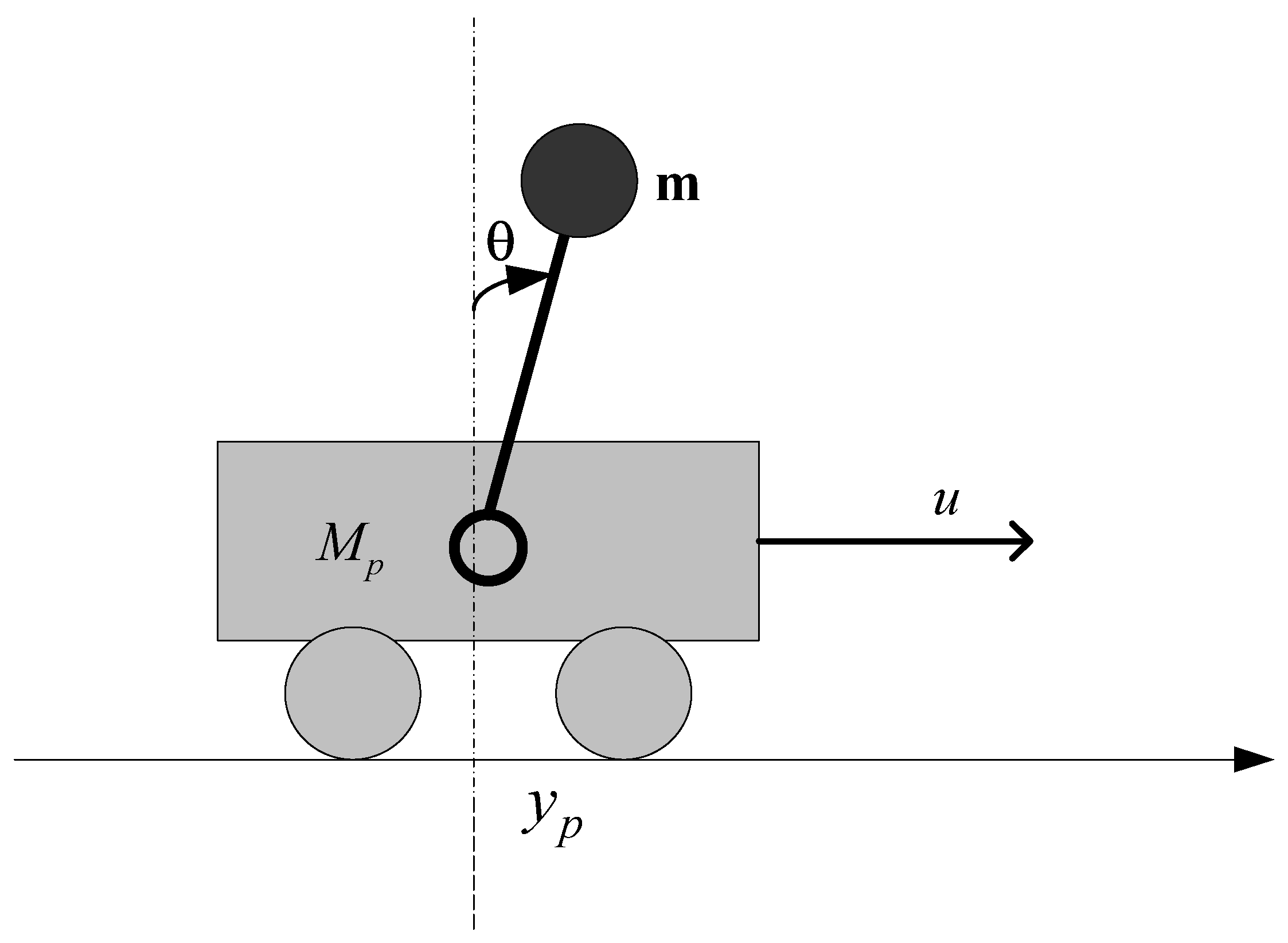
To evaluate the effectiveness of the proposed cascade control architecture integrating an Actor–Critic agent, we present a case study involving a benchmark nonlinear system: the inverted pendulum mounted on a cart (Figure 3). This system is well known in control theory for its pronounced nonlinear characteristics and non-minimum phase behavior, making it an ideal candidate for testing intelligent and adaptive control strategies.

The system consists of a horizontally moving cart of mass M, on which a pendulum of mass m and length l is hinged. The pendulum can freely swing around its pivot point. The system state is defined by four variables: the cart position x, the pendulum angle θ measured from the vertical, and their respective time derivatives $\dot{x}$ and $\dot{\theta }$. By applying Lagrange’s equations to this mechanical configuration, one obtains a set of two coupled nonlinear differential equations describing the system dynamics:

$$\left\{\begin{array}{l}\left(M+m\right)\ddot{x}+ml\ddot{\theta }cos\left(\theta \right)+ml{\dot{\theta }}^{2}sin\left(\theta \right)=u\\ l\ddot{\theta }-\ddot{x}cos\left(\theta \right)-gsin\left(\theta \right)=0\end{array}\right.$$

(26)

where u is the external control force applied to the cart, and $g=9.8 \mathrm{m}/{\mathrm{s}}^2$ is the gravitational constant. The control objective is to regulate the pendulum angle θ, which acts as a non-minimum phase output due to the unstable dynamics associated with the cart position x.

Consider $x_1$ as the output and let $x={\left[\begin{array}{cccc}\theta & \dot{\theta }& x& \dot{x}\end{array}\right]}^T$. The inverted cart–pendulum can be written as the system (1). Hence, one has the following:

$$f\left(x\right)=\left[\begin{array}{l}{x}_2\\ {\displaystyle \frac{1}{l}}\left(gsin\left(x_1\right)-{\displaystyle \frac{m\left(l{x}_2^2+gcos\left(x_1\right)\right)sin\left(x_1\right)}{M+m{\left(sin\left(x_1\right)\right)}^2}}cos\left(x_1\right)\right)\\ x_3\\ {\displaystyle \frac{m\left(l{x}_2^2+gcos\left(x_1\right)\right)sin\left(x_1\right)}{M+m{\left(sin\left(x_1\right)\right)}^2}}\end{array}\right], g\left(x\right)=\left[\begin{array}{l}0\\ {\displaystyle \frac{cos\left(x_1\right)}{M_p+m{\left(sin\left(x_1\right)\right)}^2}}\\ 0\\ {\displaystyle \frac{1}{M_p+m{\left(sin\left(x_1\right)\right)}^2}}\end{array}\right]$$

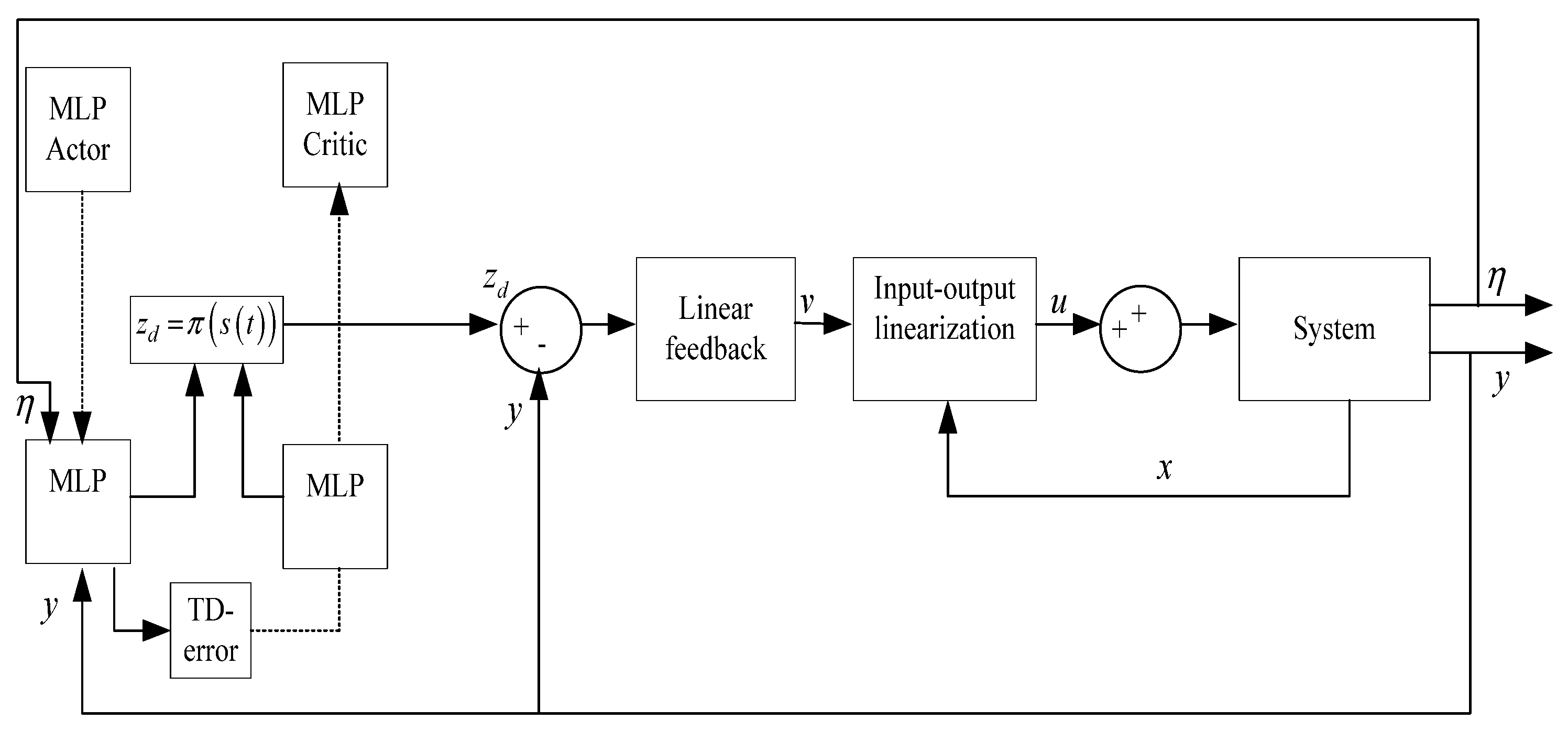
To facilitate controller design, the system is first transformed into its Byrnes–Isidori normal form, enabling the separation between the input–output dynamics, which are directly controllable, and the internal dynamics, which must be stabilized indirectly. The control input is then applied to the output θ using input–output linearization, while the internal state x is indirectly regulated through reference trajectory generation.

Two control strategies were developed and evaluated within an identical cascade control framework. The first strategy, used as a benchmark and inspired by the approach in reference [1], generates the desired trajectory z_d(t) through a conventional gradient descent algorithm, following the methodology proposed by Jouili and Benhadj Braiek [14]. In contrast, our proposed approach generates the reference signal in real time using an Actor–Critic agent trained via reinforcement learning. This agent leverages a reward function tailored to meet specific performance objectives, as outlined in Section 5. For both strategies, the inner control loop applies the same linearizing control law (22); the main difference resides in the outer loop, which defines the mechanism for reference trajectory generation.

Our approach is based on the integration of an Actor–Critic agent, trained online using a specifically designed reward function to optimize the behavior of the inverted pendulum on a cart system.

The goal of the agent is to generate a dynamic reference trajectory z_d(t) that feeds into the inner linearizing control law to stabilize the pendulum, while ensuring robustness of the internal dynamics.

i. 

Actor: MLP Producing the Intermediate Reference z_d(t)

The Actor is a Multi-Layer Perceptron (MLP) neural network, representing a parameterized policy:

$$z_d\left(t\right)={\pi }_{\theta }\left(s\left(t\right)\right)$$

(27)

where θ represents the weights and biases of the neural network.

• Input: The full system state:

$$s\left(t\right)=\left[\begin{array}{cccc}x\left(t\right)& \dot{x}\left(t\right)& \theta \left(t\right)& \dot{\theta }\left(t\right)\end{array}\right]\in {\Re }^4$$

(28)

• Output: The virtual reference $z_d\left(t\right)\in \Re$, injected into the cascade control scheme.

The typical MLP Architecture is as follows:

• Layer 1: 10 neurons with tanh activation
• Output layer: 1 neuron with linear activation

Formally:

$$\left\{\begin{array}{l}h\left(t\right)=\tanh \left(W_{1}s\left(t\right)+b_1\right)\\ z_d\left(t\right)=W_{2}h\left(t\right)+b_2\end{array}\right.$$

(29)

This output z_d(t) is passed to the control law:

$$u\left(t\right)={\displaystyle \frac{M+m\left(1-co{s}^2\left(\theta \right)\right)}{mlcos\left(\theta \right)}}\left[{\displaystyle \frac{m\mathrm{l}{\dot{\theta }}^2\sin \left(\theta \right)cos\left(\theta \right)-\sin \left(\theta \right)\left(M+m\right)}{M+m\left(1-co{s}^2\left(\theta \right)\right)}}+{\ddot{z}}_d\left(t\right)-k_1\epsilon \dot{e}-k_{0}e\right]$$

(30)

which drives the physical system.

ii. 

Critic: MLP Estimating the Value Function V(s(t))

The Critic evaluates the quality of each state s(t) by approximating the value function:

$$V^{\pi }\left(s\left(t\right)\right)\approx {\widehat{V}}_{\varphi }\left(s\left(t\right)\right)$$

(31)

where ϕ represents the Critic’s weights and biases.

• Input: s(t) $\in$ R⁴
• Output: A scalar value estimate $\widehat{V}\left(s\left(t\right)\right)\in \Re$

The typical MLP Architecture for the Critic is as follows:

• Layer 1: 20 neurons with ReLU
• Layer 2: 10 neurons with ReLU
• Output layer: 1 neuron (linear)

$${\widehat{V}}_{\varphi }\left(s\left(t\right)\right)=W_3\mathrm{Re}LU\left(\left(W_{1}s\left(t\right)+b_1\right)+b_2\right)+b_3$$

(32)

iii. 

Learning via Backpropagation—TD Update

The learning process is driven by the TD error, computed at each time step.

The Reward Function: To reflect the control objectives, the reward function is defined as

$${\widehat{V}}_{\varphi }\left(s\left(t\right)\right)=W_3\mathrm{Re}LU\left(\left(W_{1}s\left(t\right)+b_1\right)+b_2\right)+b_3$$

(33)

and TD Error as

$${\delta }_t=r\left(t\right)+\gamma \widehat{V}\left(s\left(t+1\right)\right)-\widehat{V}\left(s\left(t\right)\right)$$

(34)

with the discount factor γ = 0.99.

The weight updates:

• Critic Update:

$$\varphi \leftarrow \varphi -{\alpha }_V{\nabla }_{\varphi }\left({\delta }_t^2\right)$$

(35)

• Actor Update:

$$\theta \leftarrow \theta +{\alpha }_{\pi }{\delta }_t{\nabla }_{\theta }{\pi }_{\theta }\left(s\left(t\right)\right)$$

(36)

The gradients are obtained through automatic differentiation implemented using MATLAB 2023a.

iv. 

Online Reinforcement Learning Process

The learning is updated continuously, at every time step, using the following procedure:

a. 

Observe current state s(t)

b. 

Compute action $z_d\left(t\right)={\pi }_{\theta }\left(s\left(t\right)\right)$

c. 

Apply control u(t) using the cascade linearized control law

d. 

Simulate system to reach next state s(t + 1)

e. 

Compute reward r(t)

f. 

Compute TD error δ_t

g. 

Update Critic network (minimize ${\delta }_t^2$)

h. 

Update Actor network (maximize expected return)

The simulations were conducted using MATLAB R2023a and Simulink on a Windows 11 platform, utilizing both the Reinforcement Learning Toolbox and the Deep Learning Toolbox. The Actor–Critic agent was trained online through a custom implementation integrated into Simulink, with neural network updates managed via MATLAB 2023a scripts using the trainNetwork() function and rlRepresentation objects, with the following parameters: a cart mass of M = 1.0 kg, a pendulum mass of m = 0.1 kg, a pendulum length of l = 0.5 m, $\epsilon =0.01, k_0=4.8, k_1=6.2$, initial angle θ(0) = 0.3 rad, initial angular velocity $\dot{\theta }\left(0\right)=0 \mathrm{rad}/\mathrm{s}$, a total simulation time of 10 s, and a sampling period of 0.01 s.

The selected sampling interval is 10 ms, corresponding to a frequency of 100 Hz, which is sufficient to maintain the stability and performance of the controlled system. Both neural networks—the Actor and the Critic—are updated at each time step using discretized versions of the inputs, system states, and rewards. The continuous control signal, as defined in Equation (30), is computed at every sampling instant and then applied in a discrete manner to the simulated system operating in a closed-loop configuration. Finally, the numerical integration of the differential equations is carried out using a fixed-step solver, such as a fourth-order Runge–Kutta or an adjusted ode45, while the controller itself operates in a step-by-step mode.

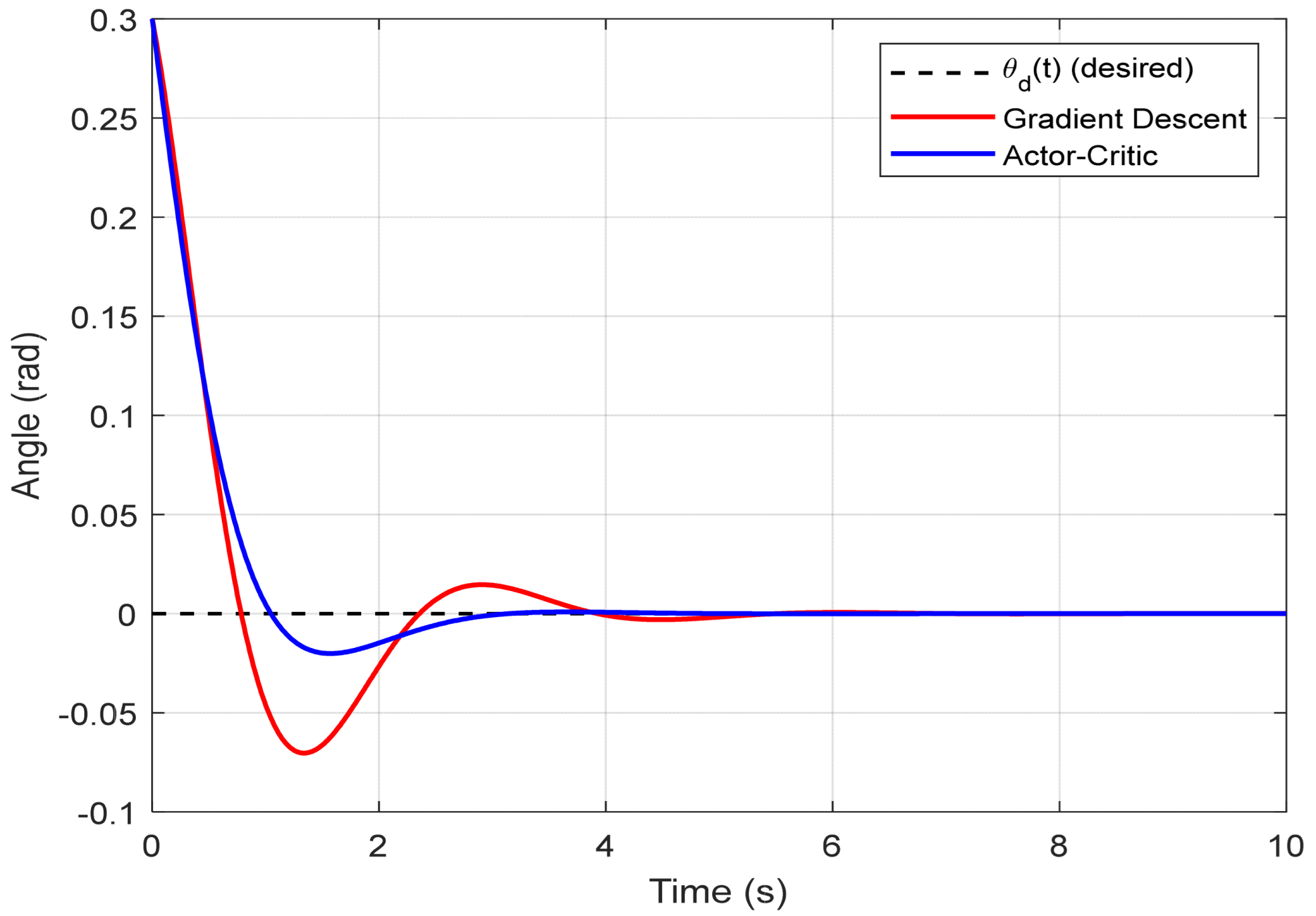
The simulation outcomes are illustrated in three comparative plots that highlight the dynamic performance of both control strategies. In Figure 4, which presents the evolution of the pendulum angle θ(t), it is evident that the Actor–Critic approach achieves faster convergence with significantly reduced oscillations compared to the gradient descent method. The pendulum under RL-based control stabilizes around the vertical position within approximately 2.1 s, whereas the gradient descent strategy requires around 3.5 s to reach a similar state, exhibiting more pronounced transient deviations.

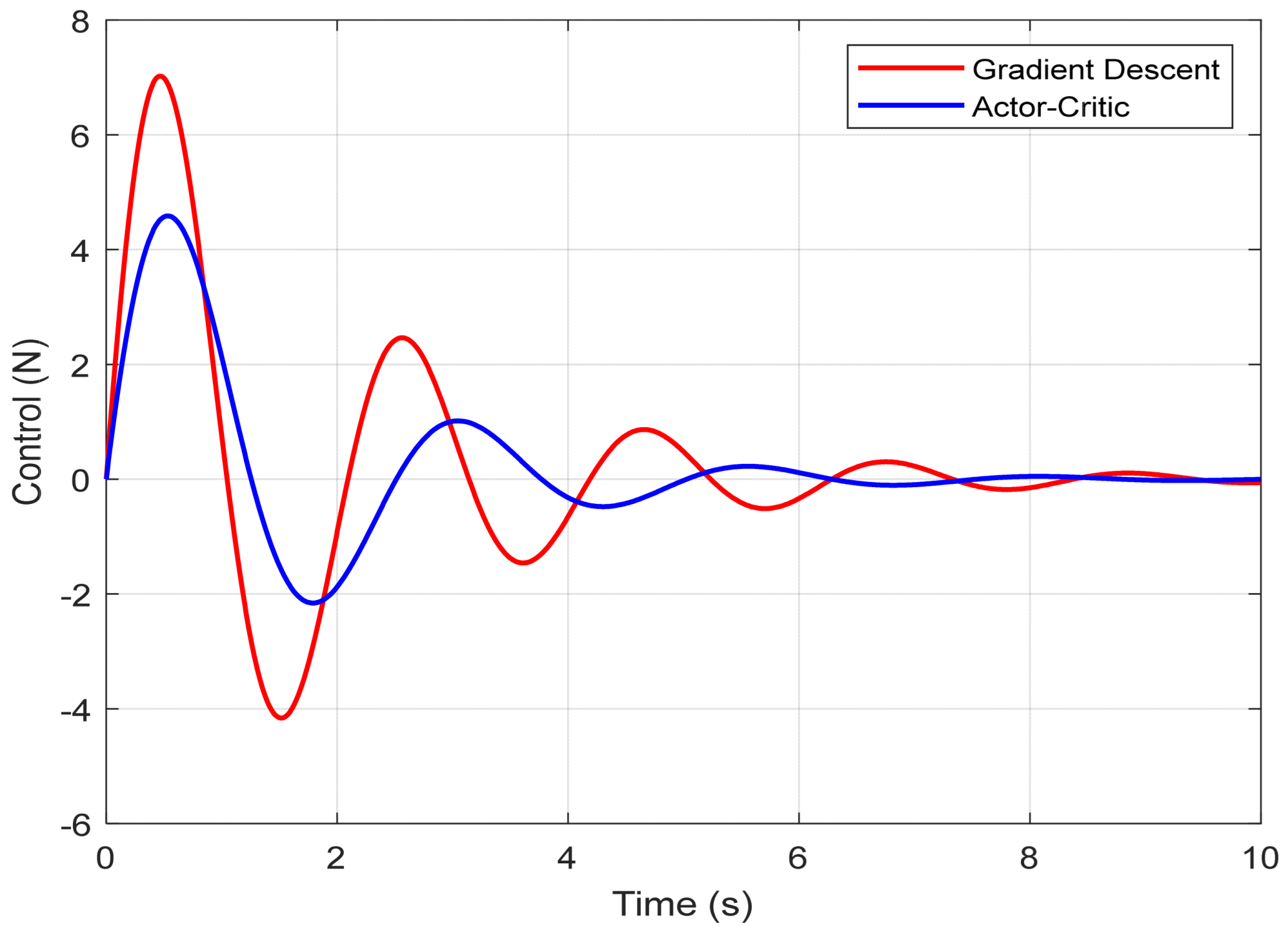
Figure 5 shows the control signal u(t) applied to the cart. The Actor–Critic agent generates a smoother and more energy-efficient control input, with lower peak magnitudes. The maximum control force produced using the RL method is approximately 6.7 newtons, while the traditional approach leads to more abrupt control actions, peaking at around 9.3 newtons. This indicates a clear advantage in terms of actuator stress and potential energy consumption when using the Actor–Critic controller.

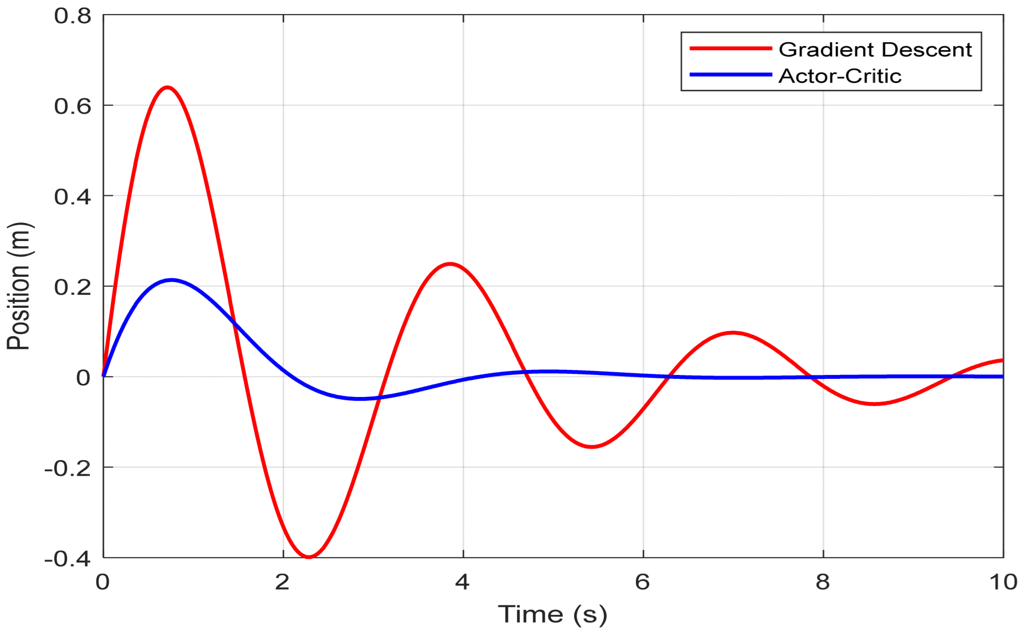
In Figure 6, the position of the cart x(t) is displayed over time. The cart displacement is better contained when using the Actor–Critic policy. The maximum lateral deviation of the cart is limited to approximately 0.55 m, compared to a more substantial swing of about 0.82 m observed with the gradient-descent-based control. This improved containment demonstrates the RL agent’s ability to better regulate the internal dynamics of the system while simultaneously stabilizing the output.

The performance of the two control strategies was evaluated based on three criteria: the mean squared error (MSE) of the pendulum angle θ(t), the maximum control effort ∣u(t)∣, and the settling time of the cart position x(t). Figure 7, Figure 8 and Figure 9 provide a quantitative comparison between the classical gradient descent method and the Actor–Critic reinforcement learning approach across these key performance metrics.

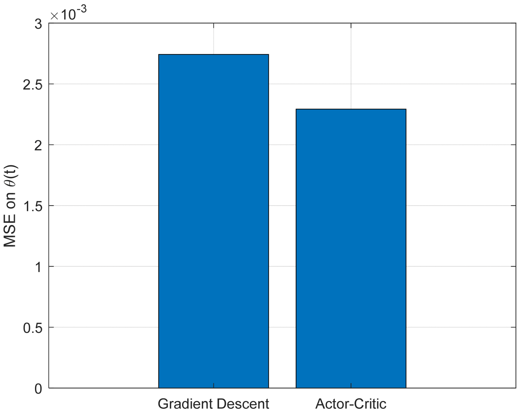
Figure 7 depicts the tracking mean squared error of the angle θ(t). It is evident that the Actor–Critic method significantly reduces the tracking error compared to the traditional approach, demonstrating improved accuracy in stabilizing the desired trajectory.

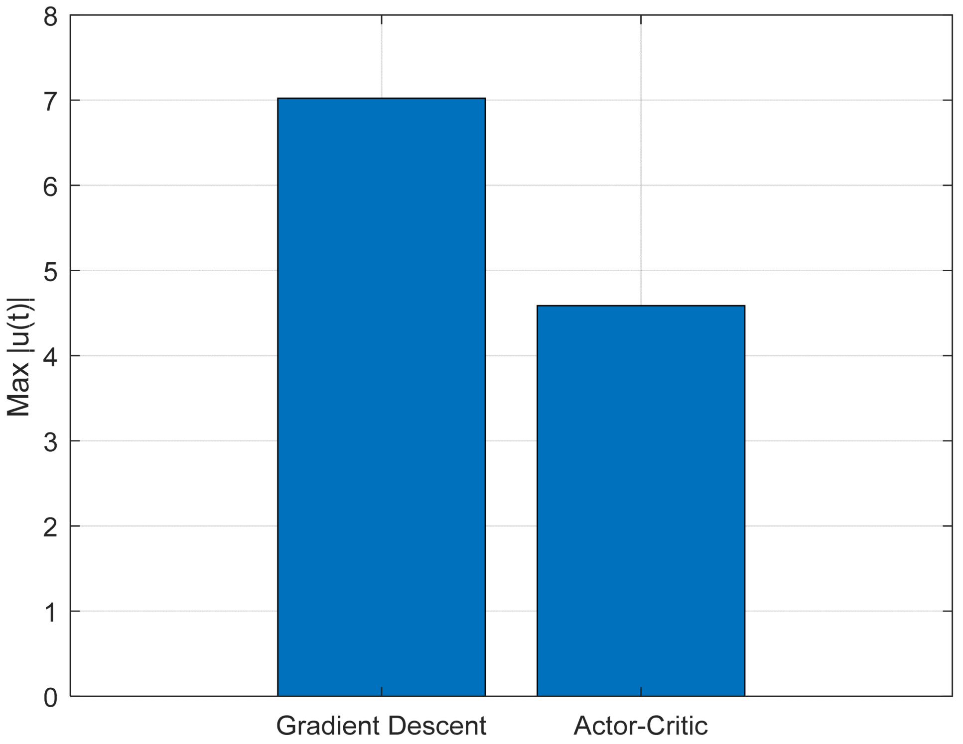
Figure 8 illustrates the maximum control effort ∣u(t)∣ produced by each method. The Actor–Critic algorithm generates a more moderate control signal, indicating a more efficient and energy-saving control action, which is advantageous for resource-constrained real-world systems.

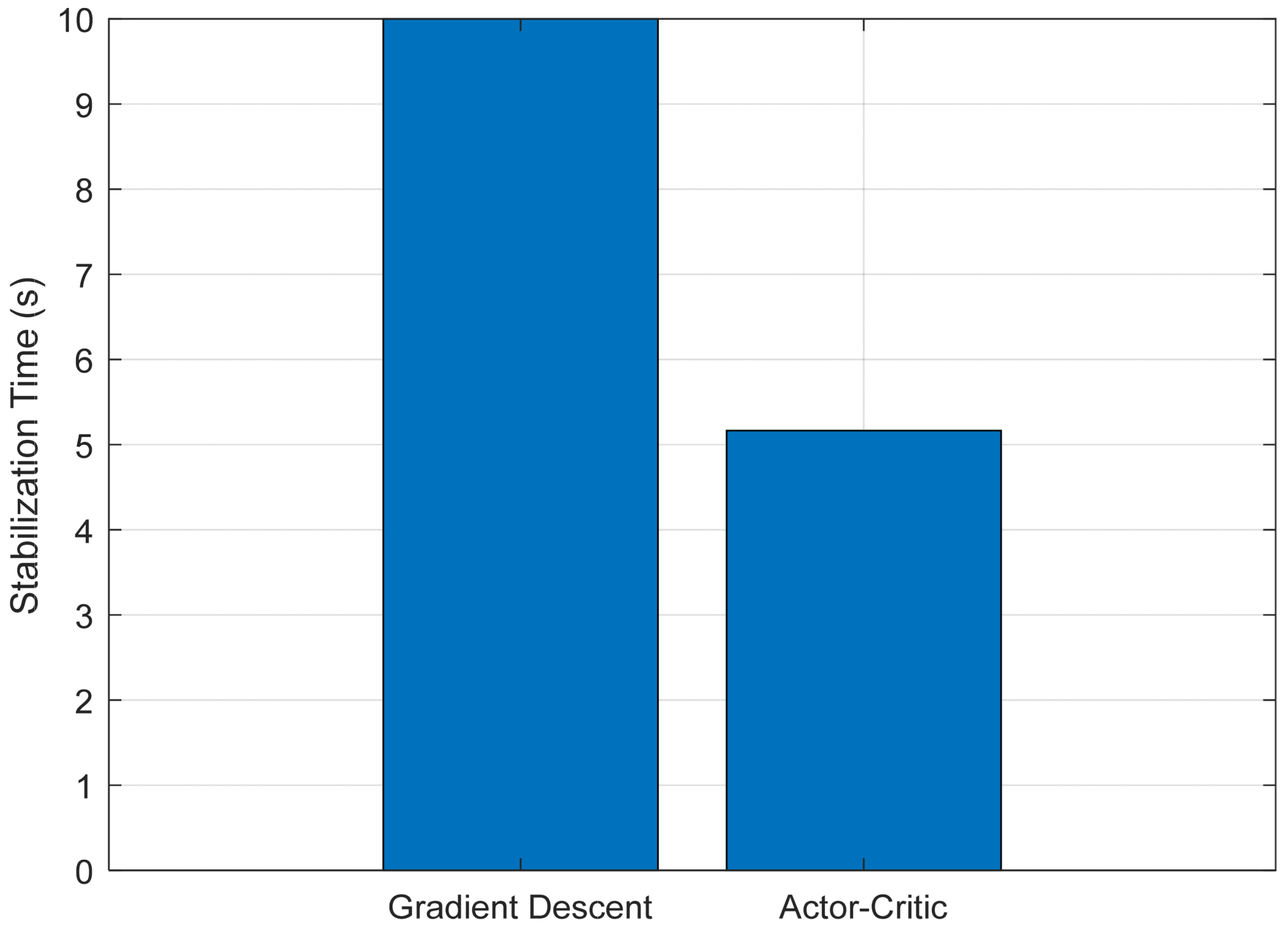
Finally, Figure 9 shows the settling time of the cart position x(t), defined as the moment after which the response remains within ±5% of its maximum amplitude. The RL-based controller achieves faster stabilization due to better damping of internal oscillations.

These results confirm the effectiveness of the Actor–Critic approach, which enhances the precision, stability, and control effort efficiency of the nonlinear system.

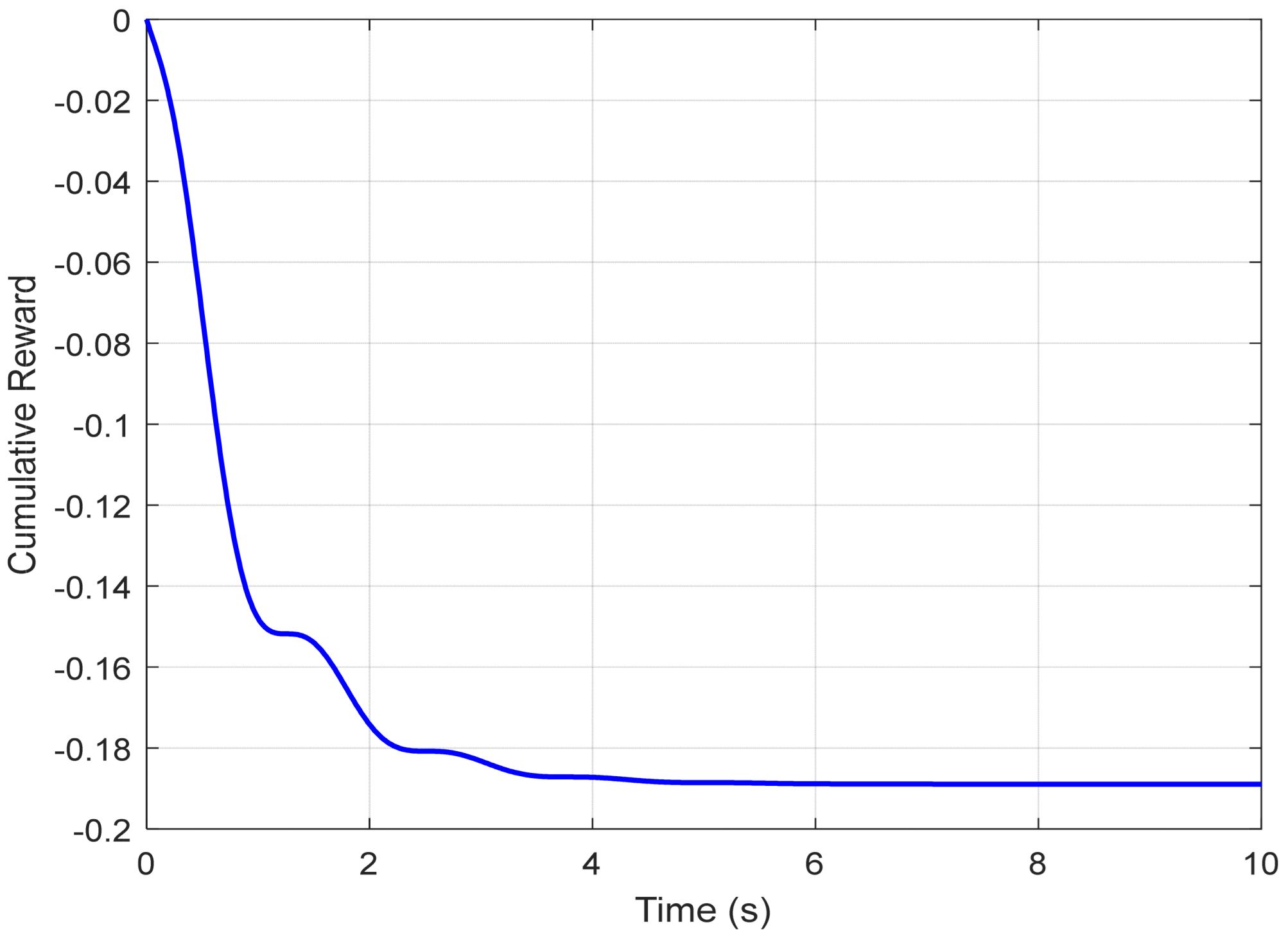
A new figure illustrates the evolution of the cumulative reward obtained by the agent over time, highlighting the gradual convergence of the learned policy toward a stable and efficient solution. Simultaneously, another plot depicts the time-varying tracking error for each control strategy, specifically comparing the Actor–Critic method and gradient descent. This visual representation enables a comparative analysis of the error magnitude, the speed of stabilization, and the overall tracking performance. To complement these visual results, quantitative indicators such as the mean squared error (MSE) have been included in a comparative table, offering an objective assessment of each approach’s effectiveness.

The presented figures provide a detailed insight into the learning dynamics and performance of the proposed control strategy. Figure 10 shows the evolution of the cumulative reward achieved by the Actor–Critic agent throughout the simulation episode. The increasing trend of this curve demonstrates the agent’s ability to progressively improve its control policy, indicating convergence toward increasingly optimal behavior.

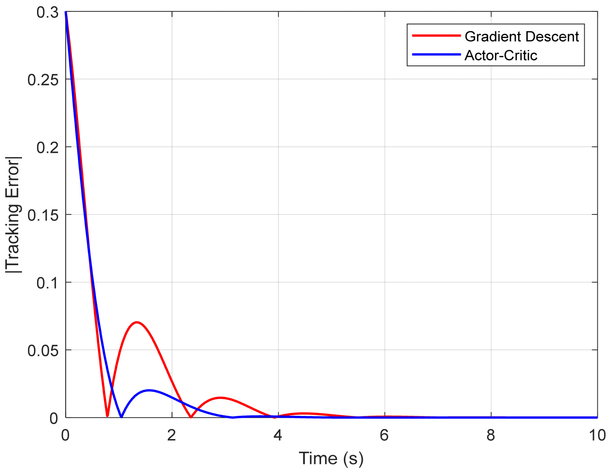
Figure 11 illustrates the absolute tracking error of the pendulum angle θ(t) with respect to the reference signal for both control strategies: gradient descent and Actor–Critic. It can be observed that the reinforcement-learning-based algorithm is able to reduce the initial error more quickly and maintain more accurate tracking over time, with fewer oscillations.

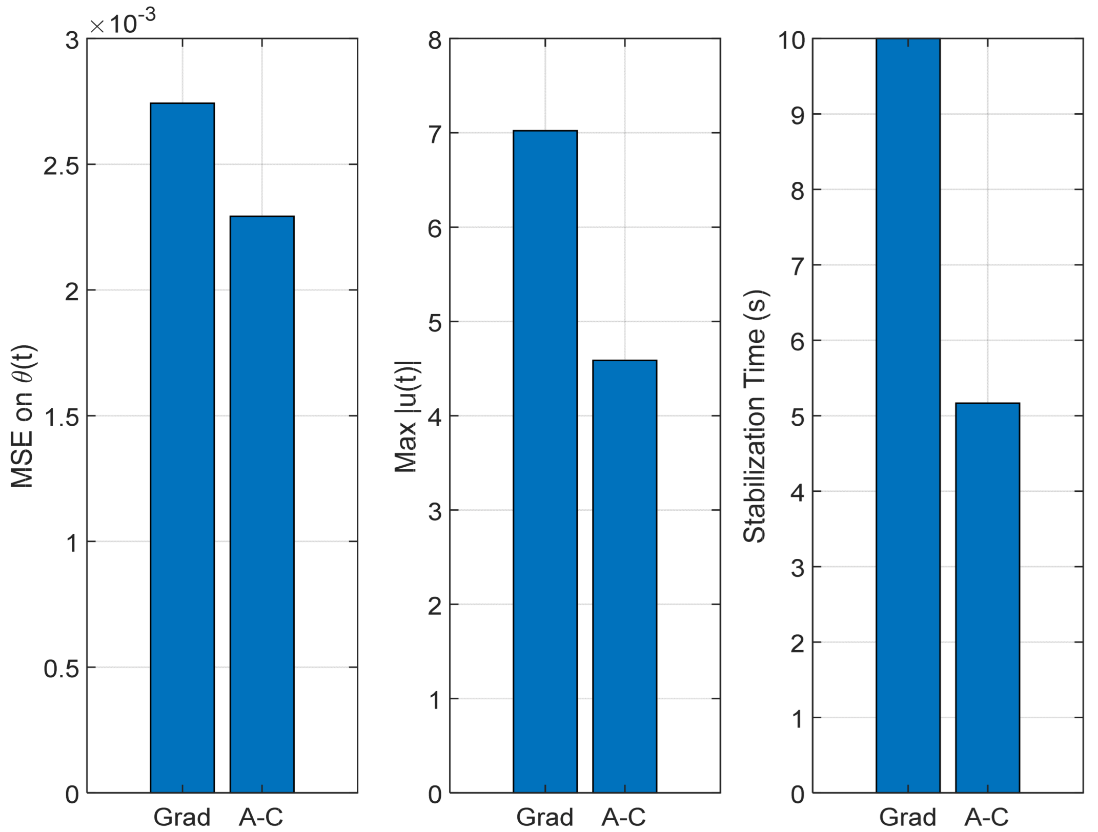
Figure 12 presents the key performance indicators used to assess the effectiveness of the proposed control approach: mean squared error (MSE), peak control effort, and stabilization time. The MSE measures how accurately the system follows the desired trajectory. The peak control effort indicates the highest level of control input applied during operation, and the stabilization time reflects how quickly the system settles into a steady state. Together, these metrics provide a well-rounded evaluation of the system’s performance in terms of precision, efficiency, and responsiveness.

7. Conclusions and Perspectives

This study introduced a novel cascade control strategy tailored to nonlinear non-minimum phase systems by embedding reinforcement learning techniques within a traditional control architecture. The core contribution lies in replacing fixed, gradient-based trajectory generation with a dynamic policy learned online by an Actor–Critic agent, enabling the system to adapt continuously to evolving conditions. The effectiveness of this approach was validated using the inverted pendulum on a cart—an established benchmark for testing nonlinear control schemes. By reformulating the system into the Byrnes–Isidori normal form, the method enabled clear decoupling between the controllable input–output dynamics and the internal dynamics, which were regulated indirectly through the learned intermediate reference signal z_d(t). Within this framework, the Actor, modeled as an MLP, was responsible for generating context-sensitive control references based on the system state, while the Critic, also implemented as an MLP, estimated the long-term performance of those decisions using temporal difference learning. The learning process was driven by a carefully designed reward function that balanced trajectory tracking, internal stability, and control efficiency. Comparative simulations confirmed that this intelligent control strategy outperformed traditional gradient-based methods across multiple dimensions, including faster stabilization, reduced oscillations, and lower actuator effort, thereby demonstrating its potential for adaptive real-time control of NNMP systems.

Building upon the promising results obtained, several directions for future research are envisioned. First, the current formulation, applied to a SISO system, can be extended to MIMO systems, where inter-channel dependencies require more advanced coordination strategies. Second, the Critic component could be further enhanced using model predictive control concepts, allowing for the integration of predictive dynamics in value estimation to better anticipate system behavior. Third, and crucially, moving from simulation to real-world experimentation—using physical testbeds such as robotic platforms, inverted pendulum rigs, or autonomous vehicles—will be essential to assess the robustness, generalization, and practical viability of the proposed method under real-time constraints and disturbances.

In conclusion, the results of this work illustrate the significant promise of combining reinforcement learning with classical nonlinear control techniques. The integration of Actor–Critic learning into a cascade control structure offers a scalable and intelligent solution for tackling the challenges of NNMP systems, paving the way for more autonomous, resilient, and energy-efficient control architectures.

References

1. Jouili, K.; Charfeddine, M.; Alquerni, M. An adaptive feedback control of nonminimum phase Boost Converter with Constant Power Load. Symmetry 2024, 16, 352–367. [Google Scholar] [CrossRef]
2. Cecconi, A.; Bin, M.; Bernard, P.; Marconi, L. On a Benchmark in Output Regulation of Non-Minimum Phase Systems. IFAC-Paper 2024, 58, 85–89. [Google Scholar] [CrossRef]
3. Elkhatem, A.S.; Engin, S.N.; Pasha, A.A.; Rahman, M.M.; Pillai, S.N. Robust Control for Non-Minimum Phase Systems with Actuator Faults: Application to Aircraft Longitudinal Flight Control. Appl. Sci. 2021, 11, 11705. [Google Scholar] [CrossRef]
4. Sun, L.; Li, D.; Gao, Z.; Yang, Z.; Zhao, S. Combined feedforward and model-assisted active disturbance rejection control for non-minimum phase system. ISA Trans. 2016, 64, 24–33. [Google Scholar] [CrossRef] [PubMed]
5. Cannon, M.; Bacic, M.; Kouvaritakis, B. Dynamic non-minimum phase compensation for SISO nonlinear affine-in-the-input systems. Automatica 2006, 42, 1969–1975. [Google Scholar] [CrossRef]
6. Isidori, A. Nonlinear Control Systems: An Introduction, 3rd ed.; Springer: Berlin/Heidelberg, Germany, 1995. [Google Scholar]
7. Hu, X.; Guo, Y.; Zhang, L.; Alsaedi, A.; Hayat, T.; Ahmad, B. Fuzzy stable inversion-based output tracking for nonlinear non-minimum phase system and application to FAHVs. J. Frankl. Inst. 2015, 352, 5529–5550. [Google Scholar] [CrossRef]
8. Khalil, H.K. Nonlinear Systems, 3rd ed.; Prentice Hall: Englewood Cliffs, NJ, USA, 2002. [Google Scholar]
9. Naiborhu, J.; Shimizu, K. Direct gradient descent control for global stabilization of general nonlinear control systems. IEICE Trans. Fundam. 2000, 83, 516–523. [Google Scholar]
10. Bortoff, S.A. Approximate state-feedback linearization using spline functions. Automatica 1997, 33, 1449–1458. [Google Scholar] [CrossRef]
11. Soroush, M.; Kravaris, C. A continuous-time formulation of nonlinear model predictive control. Int. J. Control 1996, 63, 121–146. [Google Scholar] [CrossRef]
12. Villarroel, F.A.; Espinoza, J.R.; Pérez, M.A.; Ramírez, R.O.; Baier, C.R.; Sbárbaro, D.; Silva, J.J.; Reyes, M.A. A Predictive Shortest-Horizon Voltage Control Algorithm for Non-Minimum Phase Three-Phase Rectifiers. IEEE Access 2022, 10, 107598–107615. [Google Scholar] [CrossRef]
13. Villarroel, F.A.; Espinoza, J.R.; Pérez, M.A.; Ramírez, R.O.; Baier, C.R.; Sbárbaro, D.; Silva, J.J.; Reyes, M.A. Stable Shortest Horizon FCS-MPC Output Voltage Control in Non-Minimum Phase Boost-Type Converters Based on Input-State Linearization. IEEE Trans. Energy Convers. 2021, 36, 1378–1390. [Google Scholar] [CrossRef]
14. Jouili, K.; Benhadj Braiek, N. A gradient descent control for output tracking of a class of non-minimum phase nonlinear systems. J. Appl. Res. Technol. 2016, 14, 383–395. [Google Scholar] [CrossRef]
15. Hu, J.; Liu, C.; Yang, G.H. A novel observer-based neural-network finite-time output control for high-order uncertain nonlinear systems. IEEE Trans. Neural Netw. Learn. Syst. 2023, 34, 334–347. [Google Scholar]
16. Zhang, X.; Liu, J.; Xu, X.; Yu, S.; Chen, H. Robust learning-based predictive control for discrete-time nonlinear systems with unknown dynamics and state constraints. IEEE Trans. Syst. Man Cybern. Syst. 2022, 52, 7314–7327. [Google Scholar] [CrossRef]
Figure 1. Architecture of a cascade control scheme incorporating a reinforcement learning agent based on the Actor–Critic model.
Symmetry 17 01083 g001
Figure 2. Cascade control architecture combining input–output linearization with Actor–Critic reinforcement learning.
Symmetry 17 01083 g002
Figure 3. Structural representation of the cart–pendulum system.
Symmetry 17 01083 g003
Figure 4. Pendulum angle tracking θ t : Comparison between the proposed Actor–Critic reinforcement learning method and the gradient descent approach from [14].
Symmetry 17 01083 g004
Figure 5. Control input comparison: Proposed Actor–Critic reinforcement learning method versus the gradient descent strategy from [14].
Symmetry 17 01083 g005
Figure 6. Cart position x(t): Comparison between the proposed Actor–Critic reinforcement learning strategy and the gradient descent method from [14].
Symmetry 17 01083 g006
Figure 7. Tracking accuracy: mean squared error comparison.
Symmetry 17 01083 g007
Figure 8. Comparison of maximum control inputs.
Symmetry 17 01083 g008
Figure 9. Settling time comparison for x(t) response.
Symmetry 17 01083 g009
Figure 10. Evolution of cumulative reward using the Actor–Critic algorithm.
Symmetry 17 01083 g010
Figure 11. Evolution of absolute tracking error |θ(t) − θ(ref)(t)|.
Symmetry 17 01083 g011
Figure 12. Performance metrics: mean squared error, peak control effort, and stabilization time.
Symmetry 17 01083 g012
Disclaimer/Publisher’s Note: The statements, opinions and data contained in all publications are solely those of the individual author(s) and contributor(s) and not of MDPI and/or the editor(s). MDPI and/or the editor(s) disclaim responsibility for any injury to people or property resulting from any ideas, methods, instructions or products referred to in the content.