Establishment and Identification of Fractional-Order Model for Structurally Symmetric Flexible Two-Link Manipulator System

Abstract

Integer-order models cannot characterize the dynamic behavior of the flexible two-link manipulator (FTLM) system accurately due to its viscoelastic characteristics and flexible oscillation. Hence, this paper proposes a fractional-order modeling method and identification algorithm for the FTLM system. Firstly, we exploit the memory and history-dependent properties of fractional calculus to describe the flexible link’s viscoelastic potential energy and viscous friction. Secondly, we establish a fractional-order differential equation for the flexible link based on the fractional-order Euler–Lagrange equation to characterize the flexible oscillation process accurately. Accordingly, we derive the fractional-order model of the FTLM system by analyzing the motor–link coupling as well as the symmetry of the system structure. Additionally, a system identification algorithm based on the multi-innovation integration operational matrix (MIOM) is proposed. The multi-innovation technique is combined with the least-squares algorithm to solve the operational matrix and achieve accurate system identification. Finally, experiments based on actual data are conducted to verify the effectiveness of the proposed modeling method and identification algorithm. The results show that the MIOM algorithm can improve system identification accuracy and that the fractional-order model can describe the dynamic behavior of the FTLM system more accurately than the integer-order model.

1. Introduction

The flexible two-link manipulator (FTLM) system, characterized by high flexibility, high adaptability, and lightness, is widely used in precision machining [1,2,3], intelligent manufacturing [4], medical equipment [5,6,7], aerospace [8], and other fields. Compared with rigid-link manipulators, the flexible materials used in flexible-link manipulators enable complex tasks to be performed more easily with higher precision and agility. However, FTLM systems have viscoelastic characteristics and exhibit flexible oscillations during movement [9], which makes their numerical modeling fairly complicated [10].

In recent years, extensive research has been conducted on the modeling of flexible-link manipulators. Nejad et al. [11] derived an integer-order state-space model by performing dynamic analysis on the motor and connecting rod of a flexible single-link manipulator. Alandoli et al. [12] combined the finite-element method with Euler–Lagrange equations to construct an integer-order model for a flexible single-link manipulator system. Liu et al. [13] established an integer-order model based on the Lagrangian principle and assumed-mode method by ignoring the non-linear characteristics of flexible links. Huang et al. [14] used coupled Duffing oscillators to describe the non-linear characteristics of flexible single-link manipulators and constructed an integer-order non-linear model accordingly. Loudini et al. [15] utilized the Kelvin–Voigt units to describe the viscoelastic behavior and constructed an integer-order model of a lightweight elastic link robot manipulator. Yin et al. [16] established an integer-order model for a flexible-link manipulator based on Hamilton’s principle and the assumed-mode method, considering the non-linear elastic deformation within the system. Zhang et al. [17] simplified the flexible link into a Euler–Bernoulli beam and established an FTLM model based on Hamilton’s principle.

In summary, flexible-link manipulators have mostly been analyzed using integer-order models established based on theories such as the assumed-mode method and Hamilton’s principle. However, such models oversimplify the non-linear or viscoelastic characteristics of flexible-link systems and cannot accurately characterize their flexible oscillation; thus, theoretical simulations performed using such models deviate from the actual dynamic behavior of flexible-link manipulators.

Thus far, scholars have applied the fractional-order theory to medicine, control science, and intelligent optimization. Abdoon et al. [18] used the Atangana–Baleanu Caputo fractional-order derivative operator to establish a fractional-order model of influenza. Biswas et al. [19] proposed a fractional order model of a two-link manipulator system with non-linearities. Bueno et al. [20] introduced fractional-order viscous damping coefficients and established a fractional-order model for non-linear rotational flexible structures. Cheng et al. [21] established a fractional-order model for flexible-joint robots that concisely describes the viscoelastic characteristics of such systems. Haro-Olmo et al. [22] proposed two fractional-order damping methods to describe the internal and external friction in flexible robots. Cristina et al. [23] established a fractional-order model for a flexible smart beam. Xu et al. [24] used a fractional-order derivative to describe viscoelastic effects and established a fractional-order model for a high-order viscoelastic shear beam. Wei et al. [25] proposed an improved fractional single-optimization-parameter gray model and used a genetic optimization algorithm to optimize the order of the fractional cumulants. Danca et al. [26] used the escape time algorithm adapted for the fractional-order case in the research process of the fractional-order Mandelbrot and Julia sets in the sense of q-th Caputo-like discrete fractional differences.

In addition, the Haar wavelet has a simple structure, is easy to operate, and has a fast calculation speed compared to other wavelets [27,28,29]. Moreover, the MIOM algorithm can transform the fractional-order model identification process into an algebraic equation solving problem [30,31,32,33]. By solving the algebraic equations, the fractional order and model parameters can be identified simultaneously, which simplifies the identification process and improves the identification accuracy.

The abovementioned research shows that fractional-order models can accurately describe the non-linear or viscoelasticity characteristics and dynamic behavior of flexible systems. Therefore, we leverage the history dependence and memory characteristics inherent to fractional-order calculus to establish a fractional order for the FTLM system, in addition to utilizing the multi-innovation integration operational matrix (MIOM) algorithm to identify the system’s parameters. The main contributions of this study are as follows:

• A fractional differential operator is introduced to characterize the viscoelastic potential energy and viscous friction of the FTLM system, which is more consistent with the dynamic characteristics of the FTLM system.
• A fractional-order model of the FTLM system is established based on a fractional-order Euler–Lagrange equation and the symmetry of the system structure; this model is used to describe the flexible oscillation process of the system accurately.
• A fractional-order system identification algorithm based on the MIOM is proposed. The multi-innovation technique is combined with the least-squares method to solve the FTLM system’s operational matrix and improve system identification accuracy.
• The established fractional-order model can describe the dynamic characteristics of the system more accurately than integer-order models and is more suitable for engineering applications. It can provide an accurate model for fast, accurate, and stable control of the FTLM system.

The remainder of this paper is organized as follows: Section 2 introduces the basic theory of fractional calculus. Section 3 describes the establishment of the FTLM system’s fractional-order model. Section 4 presents the MIOM algorithm-based FTLM system identification method. Section 5 details the experimental verification procedure. Finally, the conclusions are drawn in Section 6.

2. Theory of Fractional Calculus

Fractional calculus is a generalization of integer-order differentials and integrals, extending the traditional integer-order differentials or integral orders to the real-number domain. The fractional calculus operator of an arbitrary function $f(t)$ is defined as [34]

$$D^{\alpha }f(t)=\left\{\begin{array}{c}{\displaystyle \frac{d^{\alpha }}{d{t}^{\alpha }}},\\ f(t),\\ {\displaystyle \int f(t)d{t}^{-\alpha },}\end{array}\right.\begin{array}{c}\alpha >0\\ \alpha =0\\ \alpha <0\end{array}$$

(1)

where $\alpha$ represents the order of the fractional calculus operator.

Fractional calculus has three main definitions: the Grünwald–Letnikov (G-L) definition, the Riemann–Liouville (R-L) definition and the Caputo definition. These definitions are described as follows [35]:

1.

Grünwald–Letnikov (G-L) definition:

The $\alpha$-order fractional calculus of an arbitrary function $f(t)$ under the G-L definition can be expressed as

$$D^{\alpha }f(t)=\underset{h\to 0}{\lim }{\displaystyle \frac{1}{h^{\alpha }}}{\displaystyle \sum _{j=0}^{\left[\frac{t-\alpha }{h}\right]}{(-1)}^j}\left[\begin{array}{c}a\\ j\end{array}\right]f(t-jh),$$

(2)

where $\left[·\right]$ represents the rounding operation, $\left[\begin{array}{c}a\\ j\end{array}\right]={\displaystyle \frac{\mathrm{\Gamma }(\alpha +1)}{\mathrm{\Gamma }(j+1)\mathrm{\Gamma }(\alpha -j+1)}}$, and $\mathrm{\Gamma }\left(·\right)$ is the gamma function.

2.

Riemann–Liouville (R-L) definition

The fractional differential $D^{\alpha }f(t)$ of an arbitrary function $f(t)$ under the R-L definition can be expressed as

$$D^{\alpha }f(t)={\displaystyle \frac{1}{\mathsf{\Gamma }(n-a)}}{({\displaystyle \frac{d}{dt}})}^n{\displaystyle {\int }_a^t\frac{f(\tau )}{{(t-\tau )}^{\alpha -n+1}}d\tau }$$

(3)

where $\alpha$ satisfies $n-1<\alpha <n,n\in N$.

The fractional integral $I^{\alpha }f(t)$ of $f(t)$ under the R-L definition can be expressed as

$$I^{\alpha }f(t)={\displaystyle \frac{1}{\mathsf{\Gamma }(-a)}}{\displaystyle {\int }_a^t\frac{f(\tau )}{{(t-\tau )}^{\alpha +1}}d\tau }$$

(4)

3.

Caputo definition

The $\alpha$-order fractional differential of the function $f(t)$ is expressed as

$$D^{\alpha }f(t)={\displaystyle \frac{1}{\mathsf{\Gamma }(m-a)}}{\displaystyle {\int }_a^t\frac{f^{(m)}(\tau )}{{(t-\tau )}^{\alpha -m+1}}d\tau }$$

(5)

where $m=\left[\alpha \right]$ represents the integer part of $\alpha$.

The $\alpha$-order fractional integral of the function $f(t)$ is expressed as

$$I^{\alpha }f(t)={\displaystyle \frac{1}{\mathsf{\Gamma }(-a)}}{\displaystyle {\int }_a^t\frac{f(\tau )}{{(t-\tau )}^{\alpha +1}}d\tau }$$

(6)

Compared with the G-L definition, the R-L definition and the Caputo definition can avoid solving the limit problem, and the R-L definition can simplify the solution process. Herein, we use the R-L definition to establish the FTLM system’s fractional-order model.

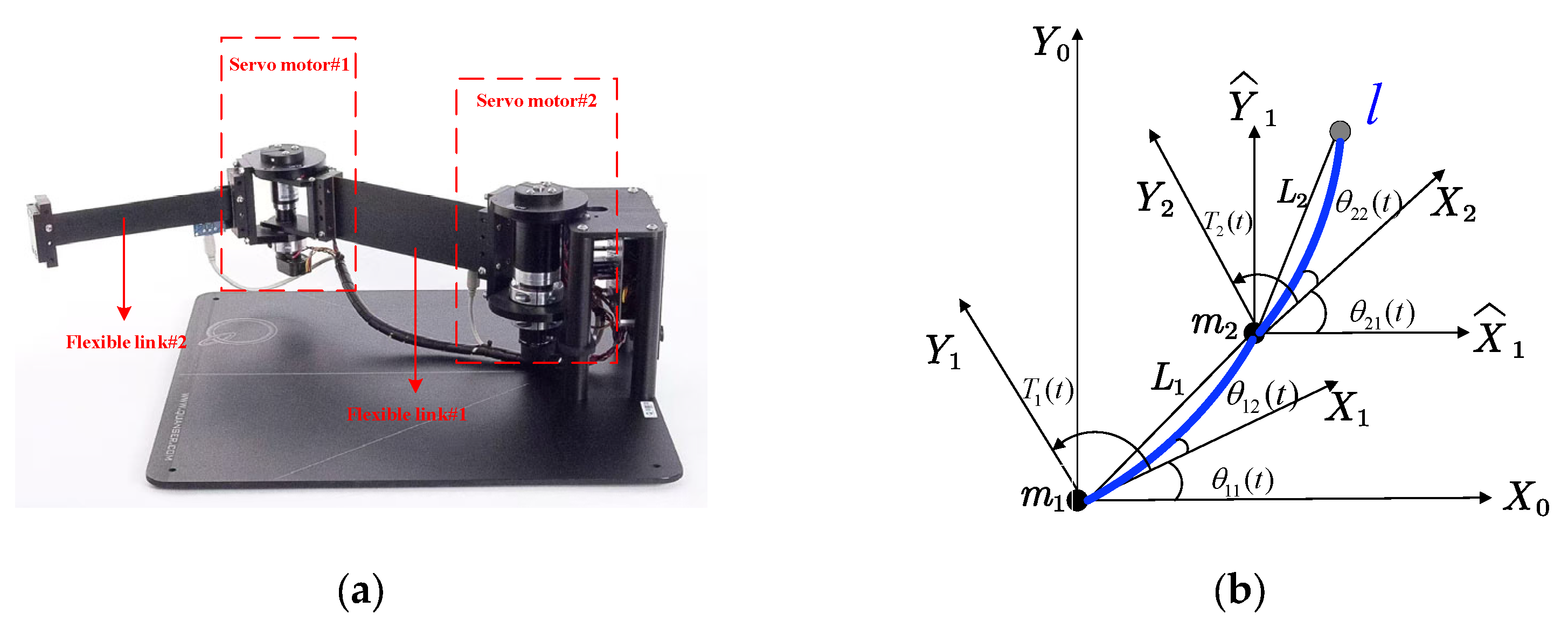
3. Establishment of the FTLM System’s Fractional-Order Model

Figure 1a shows the FTLM system. The device comprises two structurally identical servo motors and two identical flexible links. The input to the two motors is a 0.3 A current, and the outputs are two servo angles, ${\theta }_{11}(t)$ and ${\theta }_{21}(t)$. When the motors rotate, they generate torques $T_1(t)$ and $T_2(t)$, which drive the two flexible links to execute planar deflection; simultaneously, the sensors at the ends of the flexible links measure the two oscillation deflection angles, ${\theta }_{12}(t)$ and ${\theta }_{22}(t)$.

Figure 1b presents a block diagram of the FTLM system, where $X_0{Y}_0$ is the global inertial coordinate system; ${\widehat{X}}_1{\widehat{Y}}_1$ is the local inertial coordinate system centered on the second servo motor; $X_1{Y}_1$ and $X_2{Y}_2$ are the local rotating reference frames centered on the first and the second servo motors, respectively; $L_1$ and $L_2$ are the two flexible links; and the blue line $l$ represents the deformation of the two flexible links during movement.

When the motor drives the flexible link to move, the link undergoes flexible deformation, exhibiting flexible oscillation during its movement; this causes viscoelastic damping in the link’s deflection motion [15]. The history dependence and memory effects associated with fractional calculus can be used to describe the viscoelastic characteristics of flexible systems accurately [36]. Therefore, we employ fractional calculus to describe the viscoelastic characteristics of the FTLM system.

As the two servo motors and two flexible links have identical structures, we divide the FTLM system into two flexible oscillation deflection subsystems, each consisting of a motor and a flexible link, and the structures of the two subsystems are symmetrical. Taking the first subsystem as an example, we establish its fractional-order model.

According to fractional calculus and kinetic theory, the total potential energy of the first-stage subsystem equals the viscoelastic potential energy, $V_{e{T}_{12}}(t)$, of the flexible link, which can be expressed as

$$V_{e{T}_{12}}(t)={\displaystyle \frac{1}{2}}{K}_{\mathrm{s}1}{(D^{{\beta }_2}{\theta }_{12}(t))}^2,$$

(7)

where $K_{s1}$ is the viscoelastic coefficient of the flexible link and $D^{{\beta }_2}{\theta }_{12}(t)$ represents the ${\beta }_2$-order fractional differential of the oscillation deflection angle ${\theta }_{12}(t)$.

The kinetic energies of the first-stage servo motor $T_{r11}(t)$ and first-stage flexible link $T_{r12}(t)$ can be expressed as

$$\begin{array}{l}T{r}_{11}(t)={\displaystyle \frac{1}{2}}{J}_{11}{(D^{{\gamma }_1}{\theta }_{11}(t))}^2\\ T_{r12}(t)={\displaystyle \frac{1}{2}}{J}_{12}{(D^{{\gamma }_1}{\theta }_{11}(t)+D^{{\mu }_2}{\theta }_{12}(t))}^2\end{array}$$

(8)

where $J_{11}$ is the equivalent rotor moment of inertia of the first-stage harmonic drive shaft, $J_{12}$ is the moment of inertia of the first-stage flexible link, $D^{{\gamma }_1}{\theta }_{11}(t)$ represents the ${\gamma }_1$-order fractional differentials of the first-stage servo angle ${\theta }_{11}(t)$, and $D^{{\mu }_2}{\theta }_{12}(t)$ represents the ${\mu }_2$-order fractional differential of the oscillation deflection angle ${\theta }_{12}(t)$ of the first-stage flexible link.

The total kinetic energy $Tr(t)$ of the first-stage flexible oscillation deflection subsystem is the sum of $T_{r11}(t)$ and $T_{r12}(t)$.

$$\begin{array}{l}Tr(t)=T{r}_{12}(t)+T{r}_{11}(t)\\ ={\displaystyle \frac{1}{2}}{J}_{12}{(D^{{\gamma }_1}{\theta }_{11}(t)+D^{{\mu }_2}{\theta }_{12}(t))}^2+{\displaystyle \frac{1}{2}}{J}_{11}(D^{{\gamma }_1}{\theta }_{11}(t){)}^2\\ ={\displaystyle \frac{1}{2}}{J}_{12}[{(D^{{\gamma }_1}{\theta }_{11}(t))}^2+{(D^{{\mu }_2}{\theta }_{12}(t))}^2+2D^{{\gamma }_1}{\theta }_{11}(t)D^{{\mu }_2}{\theta }_{12}(t))]+{\displaystyle \frac{1}{2}}{J}_{11}{(D^{{\gamma }_1}{\theta }_{11}(t))}^2\\ =({\displaystyle \frac{1}{2}}{J}_{11}+{\displaystyle \frac{1}{2}}{J}_{12}){(D^{{\gamma }_1}{\theta }_{11}(t))}^2+J_{12}{D}^{{\mu }_2}{\theta }_{12}(t)D^{{\gamma }_1}{\theta }_{11}(t)+{\displaystyle \frac{1}{2}}{J}_{12}{(D^{{\mu }_2}{\theta }_{12}(t))}^2\end{array}$$

(9)

The non-conservative generalized force acting on the first-stage servo motor can be defined as [37]

$$\begin{array}{l}{Q}_{11}(t)=T_1(t)-B_{11}{D}^{{\gamma }_1}{\theta }_{11}(t)\\ T_1(t)=K_{\tau 1}{I}_1(t)\end{array}$$

(10)

where $B_{11}$, $K_{\tau 1}$, and $I_1(t)$ are the rotational friction coefficient, torque constant, and input current of the first-stage servo motor, respectively.

When the flexible link is in motion, viscous friction acts at the mechanical connection at the end of the link [38]. The non-conservative generalized force $Q_{12}(t)$ acting on the first-stage flexible link satisfies

$$Q_{12}(t)=-B_{12}{D}^{{\mu }_2}{\theta }_{12}(t)$$

(11)

where $B_{12}$ is the viscous friction coefficient of the first-stage flexible link.

Let $L(t)=Tr(t)-V_{e{T}_{12}}(t)$; then, according to Hamilton’s principle and the fractional-order Euler–Lagrange equation, the fractional differential equations of the first-stage servo motor and the first-stage flexible link are [39]

$$D^{{\alpha }_1-{\gamma }_1}\left[{\displaystyle \frac{\partial L(t)}{\partial D^{{\gamma }_1}{\theta }_{11}(t)}}\right]-{\displaystyle \frac{\partial L(t)}{\partial {\theta }_{11}(t)}}=Q_{11}(t)$$

(12)

$$D^{{\alpha }_2-{\mu }_2}\left[{\displaystyle \frac{\partial L(t)}{\partial D^{{\mu }_2}{\theta }_{12}(t)}}\right]-{\displaystyle \frac{\partial L(t)}{\partial D^{{\beta }_2}{\theta }_{12}(t)}}=Q_{12}(t)$$

(13)

where ${\alpha }_1>{\gamma }_1$ and ${\alpha }_2>{\mu }_2$. By substituting the total potential energy $V_{e{T}_{12}}(t)$ (Equation (7)), the total kinetic energy $Tr(t)$ (Equation (9)), the generalized force $Q_{11}(t)$ on the first-stage servo motor, and the generalized force $Q_{12}(t)$ on the first-stage flexible link into Equations (12) and (10) separately, we obtain the fractional differential equations of the first-stage flexible oscillation deflection subsystem:

$$(J_{11}+J_{12})D^{{\alpha }_1}{\theta }_{11}(t)+J_{12}{D}^{{\alpha }_1-{\gamma }_1+{\mu }_2}{\theta }_{12}(t)=K_{\tau 1}{I}_1(t)-B_{11}{D}^{{\gamma }_1}{\theta }_{11}(t)$$

(14)

$$J_{12}{D}^{{\alpha }_2-{\mu }_2+{\gamma }_1}{\theta }_{11}(t)+J_{12}{D}^{{\alpha }_2}{\theta }_{12}(t)+K_{s1}{D}^{{\beta }_2}{\theta }_{12}(t)=-B_{12}{D}^{{\mu }_2}{\theta }_{12}(t)$$

(15)

Performing ${\alpha }_1-{\beta }_1+{\beta }_0-{\alpha }_0$-order fractional differentiation on both sides of Equation (15) yields

$$J_{12}{D}^{{\alpha }_1}{\theta }_{11}(t)+J_{12}{D}^{{\alpha }_1+{\mu }_2-{\gamma }_1}{\theta }_{12}(t)+K_{s1}{D}^{{\alpha }_1-{\alpha }_2+{\mu }_2-{\gamma }_1+{\beta }_2}{\theta }_{12}(t)=-B_{12}{D}^{{\alpha }_1-{\alpha }_2+2{\mu }_2-{\gamma }_1}{\theta }_{12}(t)$$

(16)

Because a coupling relationship exists between the servo motor and the flexible link in the first-stage oscillation deflection subsystem, Equations (14) and (16) are subtracted to eliminate the common factors in the two equations. This yields the coupled fractional-order model of the servo motor in the first-stage oscillation deflection subsystem:

$$D^{{\alpha }_1}{\theta }_{11}(t)={\displaystyle \frac{K_{s1}}{J_{11}}}{D}^{{\alpha }_1-{\alpha }_2+{\mu }_2-{\gamma }_1+{\beta }_2}{\theta }_{12}(t)-{\displaystyle \frac{B_{11}}{J_{11}}}{D}^{{\gamma }_1}{\theta }_{11}(t)+{\displaystyle \frac{B_{12}}{J_{11}}}{D}^{{\alpha }_1-{\alpha }_2+2{\mu }_2-{\gamma }_1}{\theta }_{12}(t)+{\displaystyle \frac{K_{\tau 1}}{J_{11}}}{I}_1(t)$$

(17)

Similarly, by performing ${\alpha }_2-{\mu }_2+{\gamma }_1-{\alpha }_1$-order fractional differentiation on both sides of Equation (17) and substituting the result into Equation (15), we obtain the coupled fractional-order model of the flexible link in the first-stage oscillation deflection subsystem:

$$\begin{array}{l}{D}^{{\alpha }_2-{\mu }_2+{\gamma }_1}{\theta }_{11}(t)={\displaystyle \frac{K_{s1}}{J_{11}}}{D}^{{\beta }_2}{\theta }_{12}(t)-{\displaystyle \frac{B_{11}}{J_{11}}}{D}^{{\alpha }_2-{\mu }_2+2{\gamma }_1-{\alpha }_1}{\theta }_{11}(t)+{\displaystyle \frac{B_{12}}{J_{11}}}{D}^{{\mu }_2}{\theta }_{12}(t)+{\displaystyle \frac{K_{\tau 1}}{J_{11}}}{I}_1(t)\\ =-{\displaystyle \frac{B_{12}}{J_{12}}}{D}^{{\mu }_2}{\theta }_{12}(t)-D^{{\alpha }_2}{\theta }_{12}(t)-{\displaystyle \frac{K_{s1}}{J_{12}}}{D}^{{\beta }_2}{\theta }_{12}(t)\end{array}$$

(18)

Equation (18) can be rewritten as

$$D^{{\alpha }_2}{\theta }_{12}(t)=-{\displaystyle \frac{(J_{11}+J_{12})K_{s1}}{J_{11}{J}_{12}}}{D}^{{\beta }_2}{\theta }_{12}(t)+{\displaystyle \frac{B_{11}}{J_{11}}}{D}^{2{\gamma }_1-{\alpha }_1+{\alpha }_2-{\mu }_2}{\theta }_{11}(t)-{\displaystyle \frac{\left(J_{12}{B}_{12}+J_{11}{B}_{12}\right)}{J_{11}{J}_{12}}}{D}^{{\mu }_2}{\theta }_{12}(t)-{\displaystyle \frac{K_{\tau 1}{\mathrm{I}}_1(t)}{J_{11}}}$$

(19)

As the structures of the two subsystems are symmetrical, the foregoing derivation process also yields the coupled fractional-order model of the servo motor and flexible link in the second-stage oscillation deflection subsystem:

$$D^{{\alpha }_3}{\theta }_{21}(t)={\displaystyle \frac{K_{s2}}{J_{21}}}{D}^{{\alpha }_3-{\alpha }_4+{\mu }_4-{\gamma }_3+{\beta }_4}{\theta }_{22}(t)-{\displaystyle \frac{B_{21}}{J_{21}}}{D}^{{\gamma }_3}{\theta }_{21}(t)+{\displaystyle \frac{B_{22}}{J_{21}}}{D}^{{\alpha }_3-{\alpha }_4+2{\mu }_4-{\gamma }_3}{\theta }_{22}(t)+{\displaystyle \frac{K_{\tau 2}}{J_{21}}}{I}_2(t)$$

(20)

$$D^{{\alpha }_4}{\theta }_{22}(t)=-{\displaystyle \frac{(J_{21}+J_{22})K_{s2}}{J_{21}{J}_{22}}}{D}^{{\beta }_4}{\theta }_{22}(t)+{\displaystyle \frac{B_{21}}{J_{21}}}{D}^{2{\gamma }_3-{\alpha }_3+{\alpha }_4-{\mu }_4}{\theta }_{21}(t) -{\displaystyle \frac{\left(J_{22}{B}_{22}+J_{21}{B}_{22}\right)}{J_{21}{J}_{22}}}{D}^{{\mu }_4}{\theta }_{22}(t)-{\displaystyle \frac{K_{\tau 2}{I}_2(t)}{J_{21}}}$$

(21)

where $K_{\tau 2}$ is the torque constant of the first-stage servo motor. $D^{{\gamma }_3}{\theta }_{21}(t)$ and $D^{{\alpha }_3}{\theta }_{21}(t)$ represent the ${\gamma }_3$-order and ${\alpha }_3$-order fractional differentials of the second-stage servo angle ${\theta }_{21}(t)$, respectively; $D^{{\mu }_4}{\theta }_{22}(t)$, $D^{{\alpha }_4}{\theta }_{22}(t)$, and $D^{{\beta }_4}{\theta }_{22}(t)$ represent the ${\mu }_4$-order, ${\alpha }_4$-order, and ${\beta }_4$-order fractional differentials of the second-stage oscillation deflection angle ${\theta }_{22}(t)$, respectively; and $J_{22}$, $B_{22}$, and $K_{s2}$ represent the inertia moment, viscous friction coefficient, and viscoelastic coefficient of the second-stage flexible link, respectively.

The complete set of symbols is shown in

Table 1. The complete set of symbols in the modeling process.

Symbol Name	Description
${\theta }_{11}(t)$	first-stage servo angle
${\theta }_{12}(t)$	first-stage oscillation deflection angle
${\theta }_{21}(t)$	second-stage servo angle
${\theta }_{22}(t)$	second-stage oscillation deflection angle
$I_1(t)$	input current of the first-stage servo motor
$I_2(t)$	input current of the second-stage servo motor
$T_1(t)$	torque produced by first-stage servo motor
$T_2(t)$	torque produced by second-stage servo motor
$V_{e{T}_{12}}(t)$	viscoelastic potential energy of the first-stage flexible link
$T_{r11}(t)$	kinetic energies of the first-stage servo motor
$T_{r12}(t)$	kinetic energies of the first-stage flexible link
$Tr(t)$	total kinetic energy of the first-stage flexible oscillation deflection subsystem
$Q_{11}(t)$	non-conservative generalized force of the first-stage servo motor
$Q_{12}(t)$	non-conservative generalized force of the first-stage flexible link
$D^{{\alpha }_1}{\theta }_{11}(t)$	${\alpha }_1$$-\mathrm{order} \mathrm{fractional} \mathrm{differential} \mathrm{of} \mathrm{the} \mathrm{first}-\mathrm{stage} \mathrm{servo} \mathrm{angle} {\theta }_{11}(t)$
$D^{{\alpha }_2}{\theta }_{12}(t)$	${\alpha }_2$-order fractional differential of the first-stage oscillation deflection angle ${\theta }_{12}(t)$
$D^{{\alpha }_3}{\theta }_{21}(t)$	${\alpha }_3$-order fractional differential of the second-stage servo angle ${\theta }_{21}(t)$
$D^{{\alpha }_4}{\theta }_{22}(t)$	${\alpha }_4$-order fractional differential of the second-stage oscillation deflection angle ${\theta }_{22}(t)$
$D^{{\gamma }_1}{\theta }_{11}(t)$	${\gamma }_1$$-\mathrm{order} \mathrm{fractional} \mathrm{differential} \mathrm{of} \mathrm{the} \mathrm{first}-\mathrm{stage} \mathrm{servo} \mathrm{angle} {\theta }_{11}(t)$
$D^{{\gamma }_3}{\theta }_{21}(t)$	${\gamma }_3$$-\mathrm{order} \mathrm{fractional} \mathrm{differential} \mathrm{of} \mathrm{the} \sec \mathrm{ond}-\mathrm{stage} \mathrm{servo} \mathrm{angle} {\theta }_{21}(t)$
$D^{{\beta }_2}{\theta }_{12}(t)$	${\beta }_2$-order fractional differential of the first-stage oscillation deflection angle ${\theta }_{12}(t)$
$D^{{\beta }_4}{\theta }_{22}(t)$	${\beta }_4$-order fractional differential of the second-stage oscillation deflection angle ${\theta }_{22}(t)$
$D^{{\mu }_2}{\theta }_{12}(t)$	${\mu }_2$-order fractional differential of the first-stage oscillation deflection angle ${\theta }_{12}(t)$
$D^{{\mu }_4}{\theta }_{22}(t)$	${\mu }_4$-order fractional differential of the second-stage oscillation deflection angle ${\theta }_{22}(t)$

.

Based on the foregoing analysis, Equations (17) and (19)–(21) constitute the fractional-order model of the FTLM system. To simplify the expression of the FTLM system’s fractional-order model, we assume the following: in Equation (17), fractional orders ${\beta }_1={\alpha }_1-{\alpha }_2+{\mu }_2-{\gamma }_1+{\beta }_2$ and ${\mu }_1={\alpha }_1-{\alpha }_2+2{\mu }_2-{\gamma }_1$ and coefficients $a_1=K_{s1}/J_{11}$, $b_1=-B_{11}/J_{11}$, $d_1=B_{12}/J_{11}$, and $g_1=K_{\tau 1}/J_{11}$; in Equation (19), fractional order ${\gamma }_2=2{\gamma }_1-{\alpha }_1+{\alpha }_2-{\mu }_2$ and coefficients $a_2=-(J_{11}+J_{12})K_{s1}/J_{11}{J}_{12}$, $b_2=B_{11}/J_{11}$, $d_2=-\left(J_{12}{B}_{12}+J_{11}{B}_{12}\right)/J_{11}{J}_{12}$, and $g_2=-K_{\tau 1}/J_{11}$; in Equation (20), fractional orders ${\beta }_3={\alpha }_3-{\alpha }_4+{\mu }_4-{\gamma }_3+{\beta }_4$ and ${\mu }_3={\alpha }_3-{\alpha }_4+2{\mu }_4-{\gamma }_3$ and coefficients $a_3=K_{s2}/J_{21}$, $b_3=-B_{21}/J_{21}$, and $d_3=B_{22}/J_{21}$,$g_3=K_{\tau 2}/J_{21}$; in Equation (21), fractional order ${\gamma }_4=2{\gamma }_3-{\alpha }_3+{\alpha }_4-{\mu }_4$ and coefficients $a_4=-(J_{21}+J_{22})K_{s2}/J_{21}{J}_{22}$, $b_4=B_{21}/J_{21}$, $d_4=-\left(J_{22}{B}_{22}+J_{21}{B}_{22}\right)/J_{21}{J}_{22}$, and $g_4=-K_{\tau 2}/J_{21}$. Equations (17) and (19)–(21) can be simplified as follows:

$$D^{{\alpha }_1}{\theta }_{11}(t)=a_1{D}^{{\beta }_1}{\theta }_{12}(t)+b_1{D}^{{\gamma }_1}{\theta }_{11}(t)+d_1{D}^{{\mu }_1}{\theta }_{12}(t)+g_1{I}_1(t)$$

(22)

$$D^{{\alpha }_2}{\theta }_{12}(t)=a_2{D}^{{\beta }_2}{\theta }_{12}(t)+b_2{D}^{{\gamma }_2}{\theta }_{11}(t)+d_2{D}^{{\mu }_2}{\theta }_{12}(t)+g_2{I}_1(t)$$

(23)

$$D^{{\alpha }_3}{\theta }_{21}(t)=a_3{D}^{{\beta }_3}{\theta }_{22}(t)+b_3{D}^{{\gamma }_3}{\theta }_{21}(t)+d_3{D}^{{\mu }_3}{\theta }_{22}(t)+g_3{I}_2(t)$$

(24)

$$D^{{\alpha }_4}{\theta }_{22}(t)=a_4{D}^{{\beta }_4}{\theta }_{22}(t)+b_4{D}^{{\gamma }_4}{\theta }_{21}(t)+d_4{D}^{{\mu }_4}{\theta }_{22}(t)+g_4{I}_2(t)$$

(25)

Based on the above, we consider setting ${\alpha }_n={\alpha }_1,{\alpha }_2,{\alpha }_3,{\alpha }_4,$${\beta }_n={\beta }_1,{\beta }_2,{\beta }_3,{\beta }_4,$${\gamma }_n={\gamma }_1,{\gamma }_2,{\gamma }_3,{\gamma }_4,$${\mu }_n={\mu }_1,{\mu }_2,{\mu }_3,{\mu }_4,$$a_n=a_1,a_2,a_3,a_4,$$b_n=b_1,b_2,b_3,b_4,$$d_n=d_1,d_2,d_3,d_4,$ and $g_n=g_1,g_2,g_3,g_4$, so we can obtain a recursive formula for the FTLM system:

$$D^{{\alpha }_n}{\theta }_{j.x}(t)=a_n{D}^{{\beta }_n}{\theta }_{j,x}(t)+b_n{D}^{{\gamma }_n}{\theta }_{j,x}(t)+d_n{D}^{{\mu }_n}{\theta }_{j,x}(t)+g_n{I}_j(t)$$

(26)

where $D^{{\alpha }_n}{\theta }_{j,x}(t)$, $D^{{\beta }_n}{\theta }_{j,x}(t)$, $D^{{\gamma }_n}{\theta }_{j,x}(t)$, and $D^{{\mu }_n}{\theta }_{j,x}(t)$ represent the different fractional orders that need to be identified for the two servo angles ${\theta }_{11}(t)$ and ${\theta }_{21}(t)$ and the two oscillating deflection angles ${\theta }_{12}(t)$ and ${\theta }_{22}(t)$, respectively. $a_n$, $b_n$, $d_n$, and $g_n$ represent the model parameters that need to be identified. $n=1,2,3,4. j=1,2 . x=1,2$.

4. Identification of Fractional-Order FTLM System Model

Since the order of the FLTM system’s fractional-order model has changed, the parameters of the fractional-order FTLM system’s model are different from those of the integer-order model. To accurately characterize the dynamic behavior of the FTLM system and establish a precise fractional-order model, a fractional-order system identification framework based on the MIOM algorithm is proposed. This algorithm first transforms the FTLM system’s fractional-order model into an algebraic equation using a Haar wavelet-based integration operational matrix. Then, the operational matrix is solved using the multi-innovation technique combined with the least-squares method to achieve accurate system identification. Finally, the fractional order is determined using the loop-nesting method.

4.1. Haar Wavelet-Based Integration Operational Matrix

The Haar wavelet is a piecewise-constant function featuring a simple structure and fast calculation capability. Multi-scale wavelets can be generated by translating and scaling it. Haar wavelets are defined as [40]

$$h_{\sigma }(t)={\displaystyle \frac{1}{\sqrt{m}}}\left\{\begin{array}{c}{2}^{{\displaystyle \frac{\delta }{2}}}\\ -2^{{\displaystyle \frac{\delta }{2}}}\\ 0\end{array}\right. \begin{array}{c}{\displaystyle \frac{\varsigma }{2^{\delta }}}\le t<{\displaystyle \frac{\varsigma +0.5}{2^{\delta }}}\\ {\displaystyle \frac{\varsigma +0.5}{2^{\delta }}}\le t<{\displaystyle \frac{\varsigma +1}{2^{\delta }}}\\ \mathrm{elsewhere}\end{array}$$

(27)

where $m=2^{\omega }$ represents the resolution; $\sigma =1,2,\dots ,(m-1)$; $\delta$ and $\varsigma$ represent the integer decomposition of $\sigma$, respectively; $\sigma =2^{\delta }+\varsigma$; $\delta =0,1,\dots ,(\omega -1)$; $\varsigma =0,1,2,\dots ,(2^{\delta }-1)$; and $m,\sigma ,\varsigma \in Z$.

The first M terms of the arbitrary function $f(t)$ can be expanded using the following Haar wavelet:

$$f(t)={\displaystyle \sum _{i=0}^{M-1}{c}_{\sigma }}{h}_{\sigma }(t)=c_M^T{H}_M(t)$$

(28)

where $c_M\triangleq {[c_0,c_1,\dots ,c_{M-1}]}^{\mathrm{T}}$ represents the Haar wavelet coefficient vector, $H_M(t)\triangleq {[h_0(t),h_1(t)\dots h_{M-1}(t)]}^{\mathrm{T}}$ represents the Haar wavelet function vector of $f(t)$, and T and M represent the transpose and dimensions of the matrix, respectively.

Assuming $t_i={\displaystyle \frac{2i-1}{2M}}$, $i=1,2,3\dots M$, the M-square Haar matrix ${\mathbf{\Phi }}_{M\times M}$ can be expressed as

$${\mathbf{\Phi }}_{M\times M}=\left[H_M\left({\displaystyle \frac{1}{2M}}\right),H_M\left({\displaystyle \frac{3}{2M}}\right),\dots ,H_M\left({\displaystyle \frac{2M-1}{2M}}\right)\right]$$

(29)

The block pulse function (BPF) is introduced to obtain the Haar wavelet-based fractional integration operational matrix. The BPF across the interval [0, $T_f$] is defined as [41]

$${\varphi }_i(t)=\left\{\begin{array}{c}1,\\ 0,\end{array}\begin{array}{c} {\displaystyle \frac{i-1}{M}}{T}_f\le t\le {\displaystyle \frac{i}{M}}{T}_f\\ \mathrm{elsewhere}\end{array}\right.$$

(30)

The fractional integral of the BPF can be expressed as [42]

$$I^{\eta }{B}_M(t)={\mathbf{F}}_{M\times M}^{\eta }{B}_M(t)$$

(31)

where $B_M(t)={\left[{\varphi }_1(t),{\varphi }_2(t),\dots ,{\varphi }_M(t)\right]}^{\mathrm{T}}$ is the BPF basis vector and $F_{M\times M}^{\eta }$ is the M-square fractional integration operational matrix of the BPF, which is defined as [43]

$${\mathbf{F}}_{M\times M}^{\eta }={\left({\displaystyle \frac{T_f}{M}}\right)}^{\eta }{\displaystyle \frac{1}{\mathsf{\Gamma }(\eta +2)}}{\left[\begin{array}{ccccc}{v}_1& v_2& v_3& \dots & v_M\\ 0& v_1& v_2& \dots & v_{M-1}\\ ⋮& 0& v_1& \dots & v_{M-2}\\ ⋮& \ddots & 0& \dots & ⋮\\ 0& \dots & \dots & 0& v_1\end{array}\right]}_{M\times M},$$

(32)

where $v_1=1,\hspace{1em}{v}_n=n^{\eta +1}-2{(n-1)}^{\eta +1}+{(n-2)}^{\eta +1}$, and $n=2,3,\dots M$.

The Haar wavelet vector can be expressed using the Haar wavelet matrix and the BPF, as follows:

$$H_M(t)={\mathbf{\Phi }}_{M\times M}{B}_M(t)$$

(33)

By performing fractional integration on Equation (33) and combining the result with Equation (31), we can obtain

$$I^{\eta }{H}_M(t)={\mathbf{\Phi }}_{M\times M}{I}^{\eta }{B}_M(t)={\mathbf{\Phi }}_{M\times M}{\mathbf{F}}_{M\times M}^{\eta }{B}_M(t)$$

(34)

We assume that an M-square Haar wavelet-based fractional integration operational matrix $P_{\mathrm{M}\times \mathrm{M}}^{\alpha }$ exists, such that

$$I^{\eta }{H}_M(t)={\mathbf{P}}_{M\times M}^{\eta }{H}_M(t)$$

(35)

Then, combining Equation (33) with Equation (35) yields

$$I^{\eta }{H}_M(t)={\mathbf{P}}_{M\times M}^{\eta }{\mathbf{\Phi }}_{M\times M}{B}_M(t)$$

(36)

Upon substituting Equation (34) into Equation (36), $P_{\mathrm{M}\times \mathrm{M}}^{\alpha }$ can be expressed as

$${\mathbf{P}}_{M\times M}^{\eta }={\mathbf{\Phi }}_{M\times M}{\mathbf{F}}_{M\times M}^{\eta }{\mathbf{\Phi }}_{M\times M}^{-1}$$

(37)

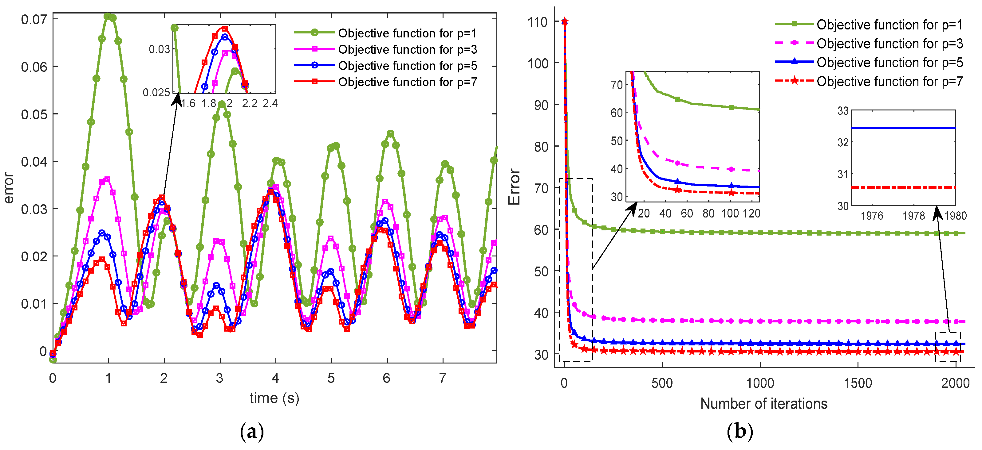
4.2. Fractional-Order FTLM System Model Identification

Considering that there are unknown parameters $a_n,b_n,d_n,g_n$ in the fractional-order recursive model of the FTLM. Assuming that ${\alpha }_n$ is the highest order in Equation (26), dividing both sides of Equation (26) by the highest-order differential yields the following fractional integral equation:

$${\theta }_{j.x}(t)=a_n{D}^{{\alpha }_n-{\beta }_n}{\theta }_{j,x}(t)+b_n{D}^{{\alpha }_n-{\gamma }_n}{\theta }_{j,x}(t)+d_n{D}^{{\alpha }_n-{\mu }_n}{\theta }_{j,x}(t)+g_n{I}^{{\alpha }_n}{I}_j(t)$$

(38)

The system input $I_j(t)$, the output servo angles, and the oscillation deflection angles ${\theta }_{j,x}(t)$ can be measured experimentally. As data on these parameters are known, they can be expanded using Haar wavelets as follows:

$$I_j(t)=U_j^T{H}_M(t), {\theta }_{j,x}(t)=Y_{j,x}^T{H}_M(t)$$

(39)

where $U_j^{\mathrm{T}}$ and $I_j(t)$ represent the Haar wavelet coefficient of the input signals $I_j(t)$ and the output signals ${\theta }_{j,x}(t)$ for the FTLM system, respectively. Substituting Equation (29) into Equation (38) and combining the result with Equation (35) yields

$$Y_{j,x}^T{H}_M(t)=a_n{Y}_{j,x}^T{\mathbf{P}}_{M\times M}^{{\alpha }_n-{\beta }_n}{H}_M(t)+b_n{Y}_{j,x}^T{\mathbf{P}}_{M\times M}^{{\alpha }_n-{\gamma }_n}{H}_M(t)+d_n{Y}_{j,x}^T{\mathbf{P}}_{M\times M}^{{\alpha }_n-{\mu }_n}{H}_M(t)+g_n{U}_j^T{\mathbf{P}}_{M\times M}^{{\alpha }_n}{H}_M(t)$$

(40)

In Equation (40), $H_M(t)$ is a Haar wavelet vector; hence, Equation (40) can be simplified to

$$Y_{j,x}^T=a_n{Y}_{j,x}^T{\mathbf{P}}_{M\times M}^{{\alpha }_n-{\beta }_n}+b_n{Y}_{j,x}^T{\mathbf{P}}_{M\times M}^{{\alpha }_n-{\gamma }_n}+d_n{Y}_{j,x}^T{\mathbf{P}}_{M\times M}^{{\alpha }_n-{\mu }_n}+g_n{U}_j^T{\mathbf{P}}_{M\times M}^{{\alpha }_n}$$

(41)

where $U_j^{\mathrm{T}}$ and $Y_{j,x}^T$ are known. The abovementioned transformation converts the fractional-order differential equation of the FTLM system into an integration operational matrix.

The MIOM algorithm-based identification framework for the FTLM system combines the multi-innovation technique with the least-squares method to solve the operational matrix. Introducing a specific innovation length accelerates the algorithm’s convergence and improves the parameter identification accuracy [30,44].

Let

$$Q=[Y_{j,x}^T{\mathbf{P}}_{M\times M}^{{\alpha }_n-{\beta }_n};Y_{j,x}^T{\mathbf{P}}_{M\times M}^{{\alpha }_n-{\gamma }_n};Y_{j,x}^T{\mathbf{P}}_{M\times M}^{{\alpha }_n-{\mu }_n};U_j^T{\mathbf{P}}_{M\times M}^{{\alpha }_n}], X=[a_n;b_n;d_n;g_n], M=Y_{j,x}^T$$

(42)

Then, the multi-innovation-based least-squares method is used to solve for the unknown parameter $X$ in the integral operation matrix, and the multi-innovation theory is used to expand $Q$ and $M$ into the following multi-innovation form:

$$\begin{array}{l}Q(p,M)={[Q(M),Q(M-1),\dots ,Q(M-p+1)]}^T;\\ M(p,M)={[M(M),M(M-1),\dots ,M(M-p+1)]}^T\end{array}$$

(43)

where $p\in Z^{+}$ is the innovation length. The multi-innovation-based least-squares algorithm for solving the integration operational matrix can be expressed as

$$\begin{array}{l}X(M)=X(M-1)+K(M)Q(p,M)J(p,M)\\ J(p,M)=M(p,M)-Q^T(p,M)X(M-1)\\ K^{-1}(M)=K^{-1}(M-1)+Q(p,M)Q^T(p,M)\end{array}$$

(44)

The unknown parameter $X=[a_n;b_n;d_n;g_n]$ in the fractional-order model of the FTLM system can be identified based on Equation (44). However, as $Q=[Y_{j,x}^T{\mathbf{P}}_{M\times M}^{{\alpha }_n-{\beta }_n};Y_{j,x}^T{\mathbf{P}}_{M\times M}^{{\alpha }_n-{\gamma }_n};Y_{j,x}^T{\mathbf{P}}_{M\times M}^{{\alpha }_n-{\mu }_n};U_j^T{\mathbf{P}}_{M\times M}^{{\alpha }_n}]$ contains unknown fractional orders, we use loop nesting to identify the unknown fractional orders ${\alpha }_n$, ${\beta }_n$, ${\gamma }_n$, and ${\mu }_n$ in $Q$.

Firstly, we define the identification interval and step size of the unknown fractional order. Secondly, we assign each order a value within this identification interval. Then, Equation (44) is solved to identify the model parameters. Thereafter, the model parameters and fractional orders are substituted into the fractional-order FTLM model (Equation (26)) to identify the output servo angles and the oscillation deflection angles ${\widehat{\theta }}_{j,x}(t)$. Finally, the fractional order of the system is changed cyclically within the identification interval. The error between the system identification output ${\widehat{\theta }}_{j,x}(t)$ and the actual output data ${\theta }_{j,x}(t)$ are compared, and the fractional order and model parameters corresponding to the minimum error are selected as the optimal solution. The error between ${\widehat{\theta }}_{j,x}(t)$ and ${\theta }_{j,x}(t)$ can be calculated using the following equation:

$$erro{r}_{j,x}(t)=\sum _{t=0}^{T_f}\left|\left.{\theta }_{j,x}(t)-{\widehat{\theta }}_{j,x}(t)\right|,\right. j=1,2, x=1,2$$

(45)

The process from physical modeling to system identification for the FTLM system is shown in Figure 2.

In the process of constructing the fractional-order model of the FTLM system, firstly, we analyze the dynamic characteristics of the FTLM system and perform a force analysis to derive its viscoelastic potential energy, kinetic energy, and generalized forces (Equations (7)–(11)). Secondly, we combine Hamilton’s principle and the fractional-order Euler–Lagrange equations to obtain the fractional-order differential equations for the FTLM system (Equations (14) and (15)). Thirdly, we obtain the coupled fractional-order model of the FTLM system based on the coupling relationship within the FTLM system (Equations (17) and (19)–(21)). Then, in order to simplify the mathematical formulation while maintaining theoretical rigor, we establish a fractional-order recursive equation to support subsequent system identification (Equation (26)). Finally, we use the MIOM algorithm (Equations (38)–(44)) to identify the unknown parameters and fractional-order degree of the FTLM system. The identification of the fractional-order model for the FTLM system can be summarized as shown in

Table 2. Identification algorithm based on the MIOM for the FTLM system.

Algorithm	Identification Algorithm Based on MIOM for FTLM System
Step 1	Collect input, $I_1(t)$ and $I_2(t)$, and output, ${\theta }_{11}(t)$, ${\theta }_{12}(t)$, ${\theta }_{21}(t)$, and ${\theta }_{22}(t)$, data.
Step 2	Determine the Haar wavelet matrix dimension, M, and generate the Haar wavelet integral operation matrix.
Step 3	Convert the FTLM system’s fractional-order model into a fractional-order integral equation using Equation (38).
Step 4	Use Equation (39) to expand the input and output data into Haar wavelets.
Step 5	Determine the system parameters to be identified, including the model parameters, fractional order, and identification interval. Cyclically change the fractional order of the system within the identification interval and use Equation (44) to identify the FTLM model parameter, $X$ .
Step 6	Substitute the model parameters and fractional orders into the fractional-order FTLM model (Equation (26)) and then calculate the error between ${\widehat{\theta }}_{j,x}(t)$ and ${\theta }_{j,x}(t)$ using Equation (45).
Step 7	Select the fractional order and model parameters corresponding to the minimum error as the optimal solution for the FTLM model.

.

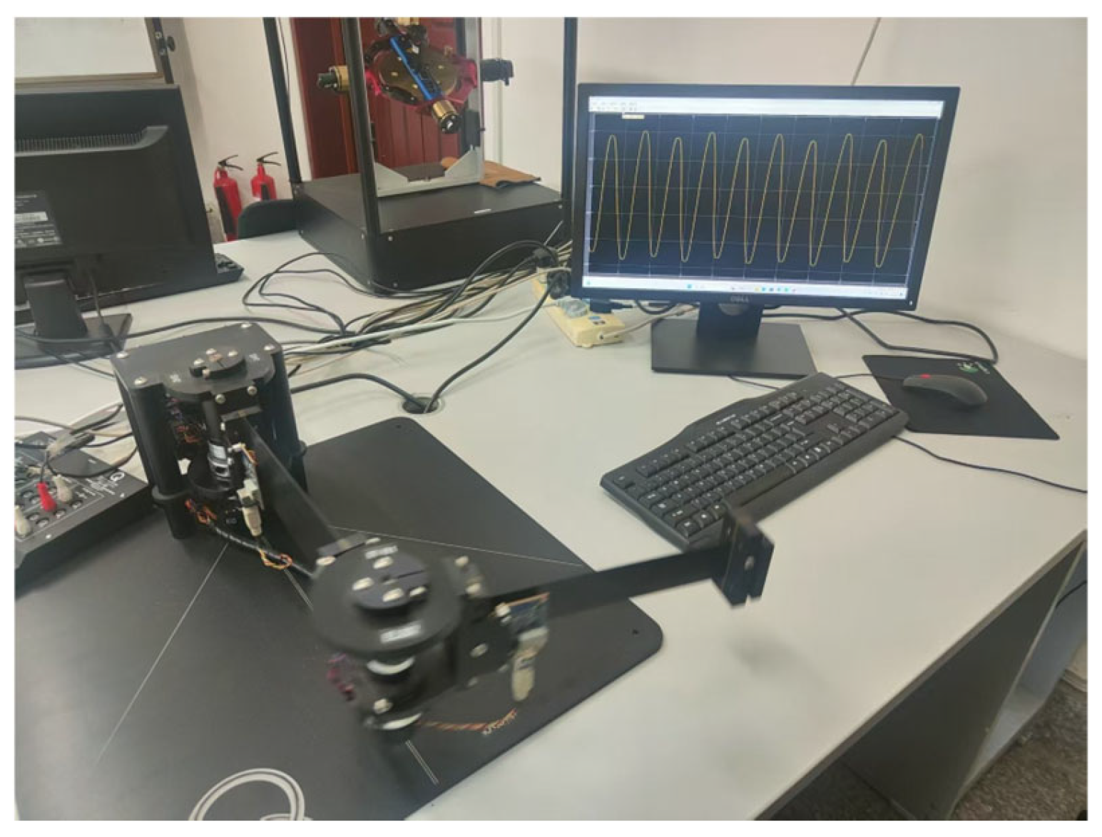
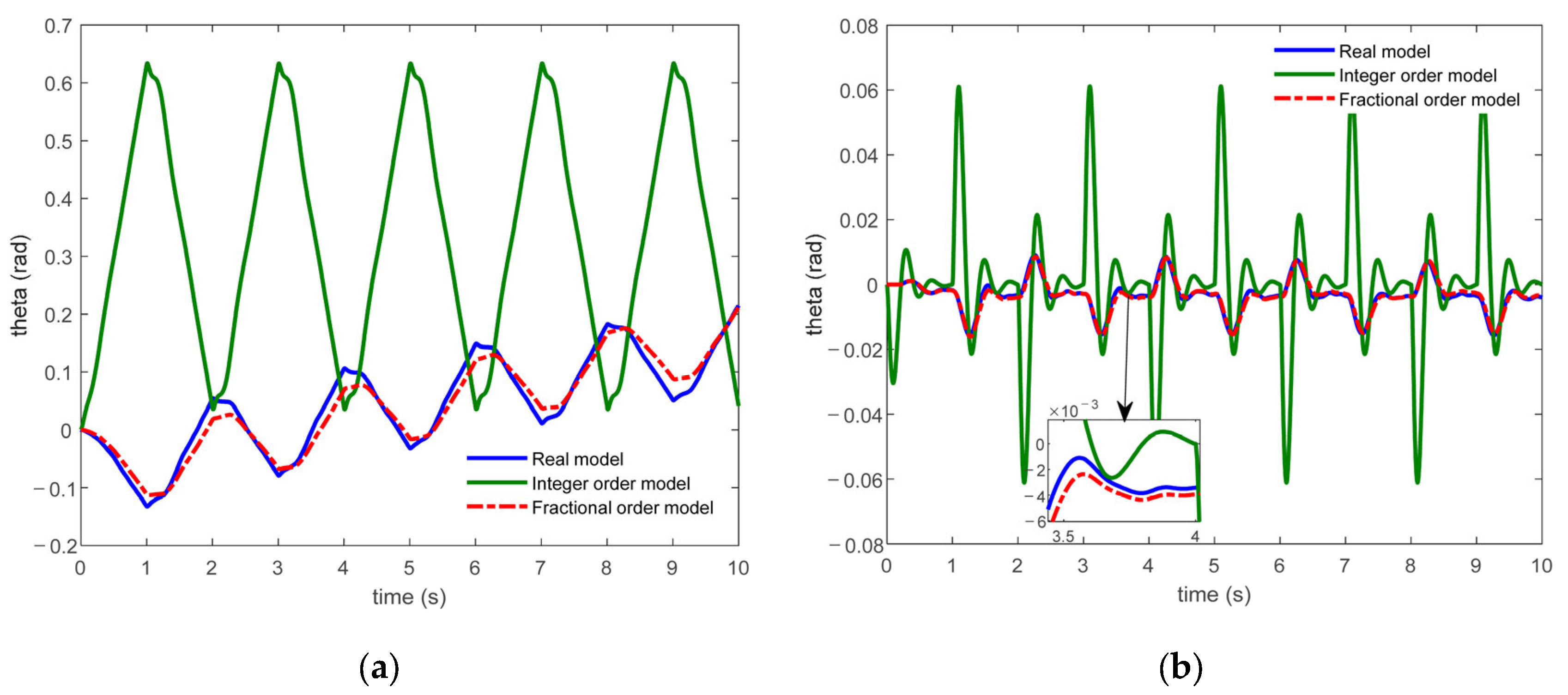
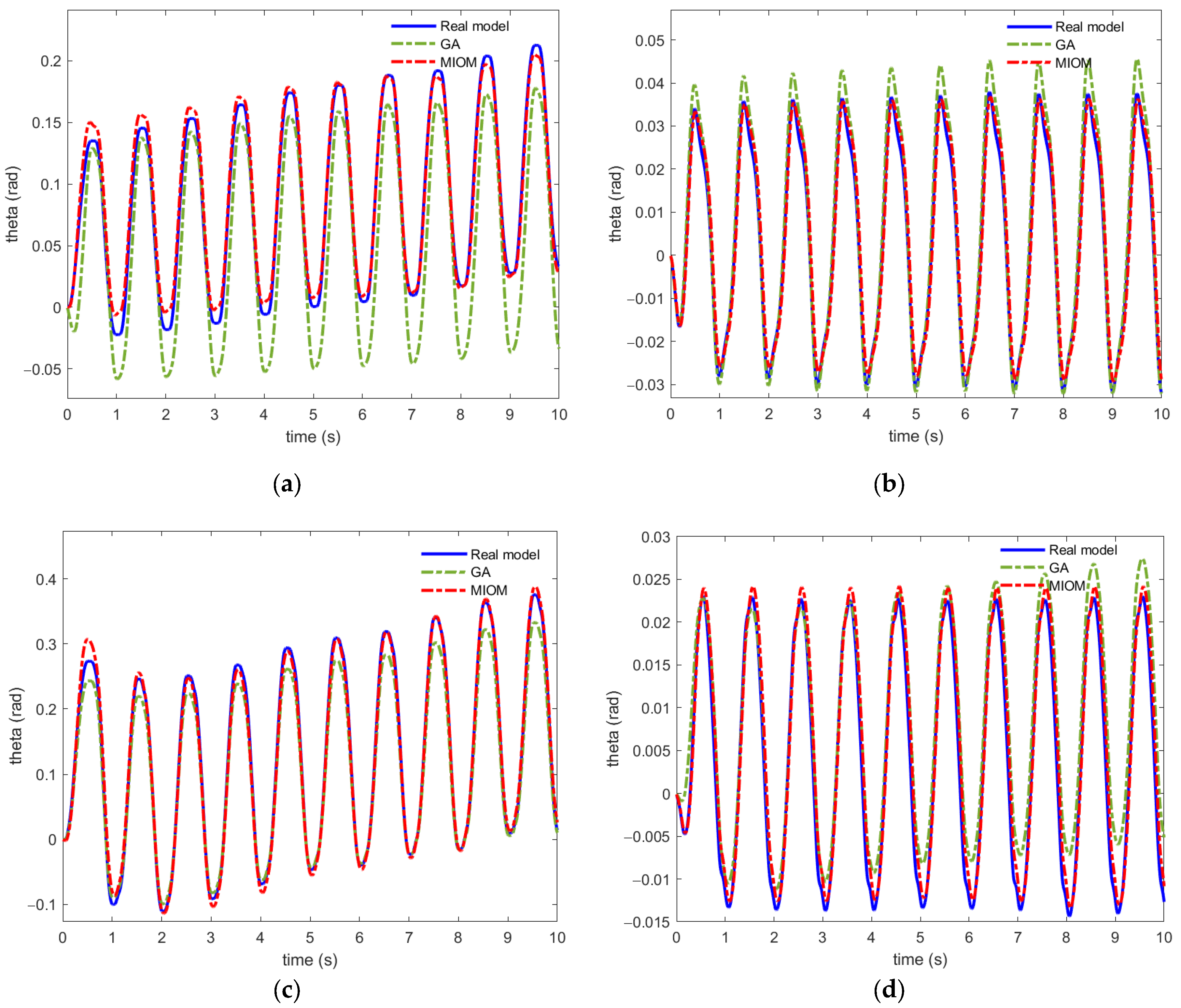
5. Experimental Verification

To verify the effectiveness of the proposed modeling method and identification algorithm, the fractional-order FTLM model is compared with the integer-order model. Figure 3 depicts the experimental verification platform, which comprises the FTLM (Quanser Inc., Markham, ON, Canada), a Q8-USB data acquisition device (Quanser Inc., Markham, ON, Canada), two servo motor angle sensors (Quanser Inc., Markham, ON, Canada), two oscillation deflection angle sensors (Quanser Inc., Markham, ON, Canada), and a PC. The operating system of this PC is Windows 11, and it is equipped with the 14th generation Core i7 processor developed by Intel. The Q-8 data acquisition device is connected to the computer via a USB 2.0 cable, and its operating voltage is 14–16 V. The digital angular position measurement of the angle sensor, using a high-resolution orthogonal optical encoder (US Digital Corporation, Vancouver, WA, USA), has 1024 lines per revolution. In the process of testing, the driving signal is input through the PC using MATLAB R2024a and QUARC (2024 SP1(24.1.4682), Quanser Inc., Markham, ON, Canada), which prompts the flexible link to undergo planar deflection. The servo angles and oscillation deflection angles are, respectively, recorded by digital angular position measurement and the strain gauge sensor and fed back to the PC through the data acquisition card. Based on the collected experimental data, the fractional-order model of the FTLM system is identified. During the experiment, we used different input signals, and each sampling time was set to 10 s. During the model configuration process, the solver type was ode1 (Euler), and the fundamental sample time was 0.002 s with a fixed step size. For the model identification process, the dimension of the Haar wavelet-based integration operational matrix was set to $\mathrm{M}=2048$. The fractional-order identification interval step size was 0.05. The hardware parameters of the FTLM system are listed in

Table 3. The parameter value of the FTLM system.

Parameter Name	Description	Value	Unit
$L_1$	length of the first-stage flexible link	0.3493	m
$L_2$	length of the second-stage flexible link	0.2975	$\mathrm{m}$
$J_{11}$	moment of inertia of the first-stage servo motor	0.0635	$\mathrm{k}\mathrm{g}{\mathrm{m}}^2$
$J_{12}$	moment of inertia of the first-stage flexible link	0.1704	$\mathrm{k}\mathrm{g}{\mathrm{m}}^2$
$B_{11}$	rotational friction coefficient of the first-stage servo motor	4.0	$\mathrm{N}{\mathrm{m}}^2$
$B_{12}$	viscous friction coefficient of the first-stage flexible link	0.421	$\mathrm{N}{\mathrm{m}}^2$
$J_{21}$	moment of inertia of the second-stage servo motor	0.003	$\mathrm{k}\mathrm{g}{\mathrm{m}}^2$
$J_{22}$	moment of inertia of the second-stage flexible link	0.0064	$\mathrm{k}\mathrm{g}{\mathrm{m}}^2$
$B_{21}$	rotational friction coefficient of the second-stage servo motor	1.5	$\mathrm{N}{\mathrm{m}}^2$
$B_{22}$	viscous friction coefficient of the second-stage flexible link	0.856	$\mathrm{N}{\mathrm{m}}^2$
$K_{s1}$	viscoelastic coefficient of the first-stage flexible link	2.69	$\mathrm{N}{\mathrm{m}}^2$
$K_{s2}$	viscoelastic coefficient of the second-stage flexible link	0.463	$\mathrm{N}{\mathrm{m}}^2$
$K_{\tau 1}$	torque constant of the first-stage servo motor	0.119	$\mathrm{N}{\mathrm{m}}^2$
$K_{\tau 2}$	torque constant of the second-stage servo motor	0.0234	$\mathrm{N}{\mathrm{m}}^2$

.

On the PC side, we input square-wave signals $I_1(t)$ and $I_2(t)$ with an amplitude of 0.3, a duty cycle of 50%, and a period of 2 s, in addition to collecting the measured output servo angles ${\theta }_{11}(t)$ and ${\theta }_{21}(t)$ and oscillation deflection angles ${\theta }_{12}(t)$ and ${\theta }_{22}(t)$. The FTLM model’s parameters and orders are identified using the MIOM algorithm, as shown in

Table 4. Identification results for first-stage flexible oscillation deflection subsystem of FTLM system.

Parameters and Orders	${\mathit{\gamma }}_1$	${\mathit{\alpha }}_1$	${\mathit{\beta }}_1$	${\mathit{\mu }}_1$	${\mathit{a}}_1$	${\mathit{b}}_1$	${\mathit{d}}_1$	${\mathit{g}}_1$	$\mathit{e}\mathit{r}\mathit{r}\mathit{o}\mathit{r}$	$\mathit{R}\mathit{M}\mathit{S}\mathit{E}$	$\mathit{N}\mathit{R}$
Integer-order models [17]	1	2	-	1	628.89	−62.956	-	140.47	640.31	0.3829	4.2028
FOM with p = 1	1.9	2	1.85	1.8	−0.5002	0.0253	0.0186	0.0345	58.973	0.0336	0.3683
FOM with p = 3	1.9	2	1.85	1.8	−0.7798	0.0339	0.0214	0.0115	37.764	0.0212	0.2323
FOM with p = 5	1.9	2	1.85	1.8	−0.8789	0.0321	0.0155	0.0029	32.426	0.0186	0.2045
FOM with p = 7	1.9	2	1.85	1.8	−0.9302	0.0277	0.0077	−0.0015	30.561	0.0180	0.1974
Parameters and Orders	${\gamma }_2$	${\alpha }_2$	${\beta }_2$	${\mu }_2$	$a_2$	$b_2$	$d_2$	$g_2$	$error$	$RMSE$	$NR$
Integer-order models [17]	1	2	-	1	−863.33	62.956	-	−140.47	23.764	0.0205	3.4665
FOM with p = 1	1.95	2	1.9	1.85	−0.7308	0.0039	−0.4494	−0.0016	1.5643	0.00097	0.1653
FOM with p = 3	1.95	2	1.9	1.85	−0.9449	0.0016	−0.2617	−0.0018	1.4834	0.00092	0.1559
FOM with p = 5	1.95	2	1.9	1.85	−1.1164	0.0011	−0.0825	−0.0018	1.3957	0.00087	0.1465
FOM with p = 7	1.95	2	1.9	1.85	−1.2655	0.0008	0.0779	−0.0017	1.3136	0.00081	0.1378

and

Table 5. Identification results for second-stage flexible oscillation deflection subsystem of FTLM system.

Parameters and Orders	${\gamma }_{\mathbf{3}}$	${\alpha }_{\mathbf{3}}$	${\beta }_{\mathbf{3}}$	${\mu }_{\mathbf{3}}$	$a_{\mathbf{3}}$	${\mathit{b}}_{\mathbf{3}}$	${\mathit{d}}_{\mathbf{3}}$	${\mathit{g}}_{\mathbf{4}}$	$\mathit{e}\mathit{r}\mathit{r}\mathit{o}\mathit{r}$	$\mathit{RMSE}$	$\mathit{NR}$
Integer-order models [17]	1	2	-	1	2271.12	−496.76	28.35	288.12	242.16	0.2312	1.6330
FOM with p = 1	1.9	2	1.85	1.8	−0.8114	0.0108	0.0067	0.0228	81.229	0.0447	0.3155
FOM with p = 3	1.9	2	1.85	1.8	−1.0049	0.0043	−0.0028	0.0395	57.369	0.0329	0.2322
FOM with p = 5	1.9	2	1.85	1.8	−1.0556	0.0048	−0.0146	0.0439	54.504	0.0321	0.2267
FOM with p = 7	1.9	2	1.85	1.8	−1.0791	0.0144	−0.0266	0.0459	53.989	0.0320	0.2266
Parameters and Orders	${\gamma }_4$	${\alpha }_4$	${\beta }_4$	${\mu }_4$	$a_4$	$b_4$	$d_4$	$g_4$	$error$	$RMSE$	$NR$
Integer-order models [17]	1	2	-	1	−3336.18	496.76	−41.65	−288.12	244.79	0.1045	29.967
FOM with p = 1	1.95	2	1.9	1.85	−0.5149	0.0053	−0.4219	−0.0006	1.1985	0.00072	0.2051
FOM with p = 3	1.95	2	1.9	1.85	−0.6531	0.0026	−0.4494	−0.0009	1.0105	0.00062	0.1781
FOM with p = 5	1.95	2	1.9	1.85	−0.7226	0.0019	−0.4173	0.0010	0.9917	0.00061	0.1756
FOM with p = 7	1.95	2	1.9	1.85	−0.7787	0.0017	−0.3759	0.0010	0.9791	0.00060	0.1737

. Figure 4, Figure 5, Figure 6, Figure 7, Figure 8 and Figure 9 present the system identification results and compare the fractional-order model (FOM) with the integer-order model. During the experiment, we incorporated the Root Mean Square Error (RMSE) and Normalized Residual (NR) to further verify the effectiveness of the method proposed in this paper.

$$RMSE=\sqrt{{\displaystyle \frac{{({\theta }_{j,x}(t)-{\widehat{\theta }}_{j,x}(t))}^2}{M}}},j=1,2, x=1,2$$

(46)

$$NR={\displaystyle \frac{e({\theta }_{j,x}(t)-{\widehat{\theta }}_{j,x}(t))}{ \sigma {\theta }_{j,x}(t)}}$$

(47)

As shown in Table 4 and Table 5, the fractional-order FTLM system model established in this study exhibits smaller errors compared to the integer-order model, which verifies the effectiveness of the proposed modeling method and MIOM algorithm. Furthermore, Figure 4 and Figure 5 show that the convergence speeds of the objective function for the servo angle ${\theta }_{11}(t)$ and deflection oscillation angle ${\theta }_{12}(t)$ gradually increase with the multi-innovation length p. For p = 7, the objective function value, RMSE, and NR are minimized, indicating that the corresponding fractional-order model more accurately characterizes the dynamic behavior of both the servo angle and the oscillations of the flexible link.

Figure 6 shows that the fractional-order model can describe the changes in the physical system—both the dynamic behavior of the servo angle and the oscillation deflection of the flexible link—in response to the square-wave input signal more accurately than the integer-order model can. This verifies the superiority of the proposed modeling method and identification algorithm in describing the dynamic characteristics of FTLM systems.

As seen in Figure 7 and Figure 8, the identification results for the fractional-order model of the second-stage subsystem are similar to those of the first-stage subsystem. As p increases, the convergence of the MIOM algorithm is gradually accelerated, the identification accuracy gradually improves, and the error between the fractional-order model and the system output in terms of ${\theta }_{21}(t)$ and ${\theta }_{22}(t)$ gradually decreases. For p = 7, the objective function values of ${\theta }_{21}(t)$ and ${\theta }_{22}(t)$ are 53.989 and 0.9791, respectively; the RMSE values are 0.0320 and 0.0006, respectively; and the NR values are 0.2266 and 0.1737, respectively, which are the smallest.

Figure 9 compares the fractional-order model with the integer-order model. The results in Figure 9 and Table 5 highlight that the integer-order model cannot characterize the dynamic behavior of ${\theta }_{21}(t)$ and ${\theta }_{22}(t)$ accurately; specifically, with regard to the flexible oscillation deflection process, the objective function error reaches 244.79. In comparison, the fractional-order model captures the dynamic behavior of the actual system more accurately. This is because the history dependence and memory effects inherent to fractional-order calculus can reflect the viscoelastic characteristics of flexible systems.

To verify the generalizability of the FTLM system’s fractional-order model, we input sine-wave signals, $I_1(t)$ and $I_2(t)$, with an amplitude of 0.6 and a frequency of 6.3 rad/s and collect the output servo angles, ${\theta }_{11}(t)$ and ${\theta }_{21}(t)$, and the oscillation deflection angles, ${\theta }_{12}(t)$ and ${\theta }_{22}(t)$. Figure 10 compares the results between the integer-order model and fractional-order models.

Figure 10 clearly shows that for both the first-stage and second-stage flexible oscillation deflection subsystems, the fractional-order model with p = 7 can characterize the dynamic behavior of the actual output servo angles, ${\theta }_{11}(t)$ and ${\theta }_{21}(t)$, and the oscillation deflection angles, ${\theta }_{12}(t)$ and ${\theta }_{22}(t)$, more accurately. The fractional-order model’s output is more consistent with the physical system’s response than the integer-order model’s output is. This confirms the generalizability and effectiveness of the proposed fractional-order modeling method and MIOM algorithm.

In order to further verify the effectiveness of the MIOM identification method, we added the FTLM fractional-order model identification method based on a genetic algorithm (GA) and compared the GA and MIOM identification results. The results are shown in Figure 11 and

Table 6. Identification results of the FTLM system by GA.

Identification Results of GA	${\mathit{\gamma }}_{\mathit{n}}$	${\mathit{\alpha }}_{\mathit{n}}$	${\mathit{\beta }}_{\mathit{n}}$	${\mathit{\mu }}_{\mathit{n}}$	${\mathit{\alpha }}_{\mathit{n}}$	${\mathit{b}}_{\mathit{n}}$	${\mathit{d}}_{\mathit{n}}$	${\mathit{g}}_{\mathit{n}}$
$n=1$	1.9299	1.9722	1.8977	1.8655	−0.2832	4.8206	−4.1504	0.0112
$n=2$	1.9621	1.9722	1.9299	1.8977	−0.0159	0.0238	0.5145	0.0172
$n=3$	1.9299	1.9722	1.8977	1.8655	−0.4537	−9.0544	9.5132	0.0006
$n=4$	1.9621	1.9722	1.9299	1.8977	−0.0231	−0.0009	0.2365	0.0012

and

Table 7. Comparison of performance indicators between GA and MIOM.

Comparison of Performance Indicators
Name of Performance Indicators	$\mathit{Error}$ $\mathit{GA}$$\mathit{MIOM}$		$\mathit{RMSE}$ $\mathit{GA}$$\mathit{MIOM}$		$\mathit{NR}$ $\mathit{GA}$$\mathit{MIOM}$
$FOM with n=1$	70.844	30.561	0.0401	0.0180	0.3554	0.1974
$FOM with n=2$	6.8453	1.3136	0.0042	0.0008	0.1812	0.1378
$FOM with n=3$	65.306	53.989	0.0395	0.0320	0.2270	0.2266
$FOM with n=4$	7.3449	0.9791	0.0042	0.0006	0.3058	0.1737

.

Figure 11 shows that the MIOM algorithm is superior to the GA, and the fractional-order model constructed by it can more accurately represent the dynamic characteristics of the FTLM system. Furthermore, the error, RMSE and NR of the MIOM algorithms are all lower than the GA’s. Based on this, we further verified the superiority of MIOM algorithms for identifying the fractional-order system of an FTLM.

6. Conclusions

This paper proposes a fractional-order modeling method for the FTLM system, along with the MIOM algorithm for system identification. Firstly, a fractional differential operator is used to describe the viscoelastic properties of the flexible link. Secondly, a fractional-order differential equation for the flexible link is established to characterize the flexible oscillation process accurately. Then, the FTLM system’s fractional-order model is derived by utilizing the coupling relationship between the motor and the flexible link. To achieve system identification, the FTLM system is transformed into a Haar wavelet-based integral operation matrix, which is solved by combining the multiple-innovation technique with the least-squares method. Finally, experiments are conducted to verify the effectiveness of the proposed modeling method and system identification algorithm. The results show that, compared with the integer-order model, the fractional-order model can describe the viscoelastic characteristics of the FTLM system more accurately in terms of both the dynamic behavior of the servo angle and the oscillation deflection angle. Additionally, with regard to system identification based on the MIOM algorithm, increasing the multi-innovation length gradually improves the identification accuracy of the FTLM model’s parameters and accelerates the algorithm’s convergence. Thus, the proposed model can enable fast, accurate, and stable control of FTLM systems. Moreover, the MIOM algorithm can be extended to non-linear fractional-order systems or other complex fractional-order systems, such as heat transfer systems, engineering control system, and wind power systems. Future research will focus on designing active vibration suppression strategies for the flexible oscillations existing in the FTLM system, including but not limited to the design of two-layer control strategies based on disturbance observers and the fractional-order control strategy design based on extended state observers. It is particularly important to note that in the design of vibration suppression control strategies, applying the defined torque input during the system’s response state can help better evaluate the accuracy and the stability of the control system

References

1. Dehkordi, S.F. Dynamic analysis of flexible-link manipulator in underwater applications using Gibbs-Appell formulations. Ocean Eng. 2021, 241, 110057. [Google Scholar] [CrossRef]
2. Pu, Y.X.; Li, X.B.; Zhang, F. Hybrid control of piezoelectric flexible manipulator based on Volterra filtered-xLMS algorithm. J. Vib. Control 2023, 29, 185–199. [Google Scholar] [CrossRef]
3. Mo, H.J.; Wei, R.F.; Bo, O.Y.; Xing, L.X.; Shan, Y.H.; Liu, Y.H.; Sun, D. Control of a flexible continuum manipulator for laser beam steering. IEEE Rob. Autom. Lett. 2021, 6, 1074–1081. [Google Scholar] [CrossRef]
4. Chen, X.A. The computational design of a fractal-inspired soft robotic. Alex. Eng. J. 2023, 84, 37–46. [Google Scholar] [CrossRef]
5. Ma, X.; Wang, P.; Ye, M.X.; Chiu, P.W.Y.; Li, Z. Shared autonomy of a flexible manipulator in constrained endoluminal surgical tasks. IEEE Rob. Autom. Lett. 2019, 4, 3106–3112. [Google Scholar] [CrossRef]
6. Mehedi, I.M.; Rao, K.P. Surgical robotic arm control for tissue ablation. J. Robot. Surg. 2020, 14, 881–887. [Google Scholar] [CrossRef]
7. Kim, J.; de Mathelin, M.; Ikuta, K.; Kwon, D.S. Advancement of flexible robot technologies for endoluminal surgeries. Proc. IEEE 2022, 110, 909–931. [Google Scholar] [CrossRef]
8. Qiao, J.Z.; Wu, H.; Yu, X. High-precision attitude tracking control of space manipulator system under multiple disturbances. IEEE Trans. Syst. Man Cybern. Syst. 2019, 51, 4274–4284. [Google Scholar] [CrossRef]
9. Ranjan, R.; Dwivedy, S.K. Dynamic analysis of flexible manipulators, a literature review. Mech. Mach. Theory 2006, 41, 749–777. [Google Scholar] [CrossRef]
10. Subudhi, B.; Morris, A.S. Dynamic modelling, simulation and control of a manipulator with flexible links and joints. Rob. Auton. Syst. 2002, 41, 257–270. [Google Scholar] [CrossRef]
11. Nejad, F.H.; Fayazi, A.; Zadeh, H.G.; Marj, H.F.; HosseinNia, S.H. Precise tip-positioning control of a single-link flexible arm using a fractional-order sliding mode controller. J. Vib. Control 2020, 26, 1683–1696. [Google Scholar] [CrossRef]
12. Alandoli, E.A.; Lee, T.S.; Lin, Y.J.; Vijayakumar, V. Dynamic model and intelligent optimal controller of flexible link manipulator system with payload uncertainty. Arab. J. Sci. Eng. 2021, 46, 7423–7433. [Google Scholar] [CrossRef]
13. Liu, J.Q.; Li, X.P.; Yin, M.; Wei, L.; Wang, H.Z. Modeling and Rotation Control Strategy for Space Planar Flexible Robotic Arm Based on Fuzzy Adjustment and Disturbance Observer. Mathematics 2024, 12, 2513. [Google Scholar] [CrossRef]
14. Huang, J.; Ji, J.C. Vibration control of coupled Duffing oscillators in flexible single-link manipulators. J. Vib. Control 2021, 27, 2058–2068. [Google Scholar] [CrossRef]
15. Loudini, M.; Boukhetala, D.; Tadjine, M.; Boumehdi, M.A. Application of Timoshenko beam theory for deriving motion equations of a lightweight elastic link robot manipulator. Int. J. Autom. Robot. Auton. Systems. 2006, 5, 11–18. [Google Scholar]
16. Yin, H.B.; Li, Y.G.; Li, J.F. Decomposed dynamic control for a flexible robotic arm in consideration of nonlinearity and the effect of gravity. Adv. Mech. Eng. 2017, 9, 1687814017694104. [Google Scholar] [CrossRef]
17. Zhang, S.; Zhao, X.N.; Liu, Z.J.; Li, Q. Boundary torque control of a flexible two-link manipulator and its experimental investigation. IEEE Trans. Ind. Electron. 2020, 68, 8708–8717. [Google Scholar] [CrossRef]
18. Abdoon, M.A.; Saadeh, R.; Berir, M.; EL Guma, F.; Ali, M. Analysis, modeling and simulation of a fractional-order influenza model. Alex. Eng. J. 2023, 74, 231–240. [Google Scholar] [CrossRef]
19. Biswas, D.; Sharma, K.D. Real-time fractional order φ1 adaptive control strategy for fractional order two link manipulator. Phys. Scr. 2024, 99, 075272. [Google Scholar] [CrossRef]
20. Bueno, A.M.; Daltin, D.C.; Serni, P.J.A.; Balthazar, J.M.; Tusset, A.M. Suboptimal State Tracking Control Applied to a Nonlinear Fractional-Order Slewing Motion Flexible Structure. J. Comput. Nonlinear Dyn. 2022, 17, 091005. [Google Scholar] [CrossRef]
21. Cheng, C.; Shen, H.k. Fractional-order dynamics and adaptive dynamic surface control of flexible-joint robots. Asian J. Control 2023, 25, 3029–3044. [Google Scholar] [CrossRef]
22. Haro-Olmo, M.I.; Tejado, I.; Vinagre, B.M.; Feliu-Batlle, V. Fractional-Order Models of Damping Phenomena in a Flexible Sensing Antenna Used for Haptic Robot Navigation. Fractal Fract. 2023, 7, 621. [Google Scholar] [CrossRef]
23. Muresan, C.I.; Folea, S.; Birs, I.R.; Ionescu, C. A novel fractional-order model and controller for vibration suppression in flexible smart beam. Nonlinear Dyn. 2018, 93, 525–541. [Google Scholar] [CrossRef]
24. Xu, Y.Q.; Wei, P.J. Dynamic response of fractional-order viscoelastic high-order shear beam based on nonlocal strain gradient elasticity. Acta Mech. Solida Sin. 2023, 36, 875–883. [Google Scholar] [CrossRef]
25. Wei, J.T.; Wu, Y.H. Improved Fractional Order Single Optimization Parameter Grey Model. J. Grey System. 2023, 35, 154–171. [Google Scholar]
26. Danca, M.F.; Feckan, M. Mandelbrot set and Julia sets of fractional order. Nonlinear Dyn. 2023, 111, 9555–9570. [Google Scholar] [CrossRef]
27. Cattani, C. Haar wavelet fractional derivative. Proc. Est. Acad. Sci. 2022, 71, 55–64. [Google Scholar] [CrossRef]
28. Arafa, H.M.; Ramadan, M.A.; Althobaiti, N.A. Numerical Technique Based on Bernoulli Wavelet Operational Matrices for Solving a Class of Fractional Order Differential Equations. Fractal Fract. 2023, 7, 604. [Google Scholar] [CrossRef]
29. Shree, R.V.; Mallikarjun, B.P.; Souayeh, B.; Bhattacharya, S. Application of fibonacci wavelet frame operational matrix for the analysis of arrhenius-controlled heat transfer flow in a microchannel. Case Stud. Therm. Eng. 2024, 63, 105326. [Google Scholar] [CrossRef]
30. Wang, Z.S.; Liang, S.N.; Chen, B.C.; Sun, H.L. Identification of fractional order time delay system with measurement noise using variable period integration operational matrix. Mech. Syst. Sig. Process. 2025, 223, 111930. [Google Scholar] [CrossRef]
31. Shiralashetti, S.C.; Pala, V.R.; Hanaji, S.I. Legendre wavelet integration operational matrix method for the numerical solution of unsteady MHD nanofluid flow between moving parallel plates. Numer. Heat Transfer, Part B 2024, 1–24. [Google Scholar] [CrossRef]
32. Wang, Y.X.; Zhu, L.; Hu, D.L. Euler wavelets operational matrix of integration and its application in the calculus of variations. Int. J. Comput. Math. 2024, 101, 386–406. [Google Scholar] [CrossRef]
33. Turan-Dincel, A.; Tural-Polat, S.N. Operational matrix method approach for fractional partial differential-equations. Phys. Scr. 2024, 99, 125254. [Google Scholar] [CrossRef]
34. Podlubny, I. Fractional Differential Equations; Academic Press: Cambridge, MA, USA, 1999. [Google Scholar]
35. Podlubny, I. Geometrical and physical interpretation of fractional integration and fractional diggerentiation. Fract. Calc. Appl. Anal. 2002, 5, 357–366. [Google Scholar]
36. Chen, B.; Li, C.Y.; Wilson, B.; Huang, Y.J. Fractional modeling and analysis of coupled MR damping system. IEEE/CAA J. Autom. Sin. 2016, 3, 288–294. [Google Scholar] [CrossRef]
37. Zhu, J.W.; Chen, D.Y.; Zhao, H.; Ma, R.F. Nonlinear dynamic analysis and modeling of fractional permanent magnet synchronous motors. J. Vib. Control 2016, 22, 1855–1875. [Google Scholar] [CrossRef]
38. Lazarevic, M.P.; Mandić, P.D.; Ostojic, S. Further results on advanced robust iterative learning control and modeling of robotic systems. J. Mech. Eng. Sci. 2021, 235, 4719–4734. [Google Scholar] [CrossRef]
39. Lavin-Delgado, J.E.; Solis-Perez, J.E.; Gomez-Aguilar, J.F.; Escobar-Jimenez, R.F. Trajectory tracking control based on non-singular fractional derivatives for the PUMA 560 robot arm. Multibody Sys. Dyn. 2020, 50, 259–303. [Google Scholar] [CrossRef]
40. Jiang, G.; Ke, T.; Deng, M.T. Least square method based on Haar wavelet to solve multi-dimensional stochastic Itô-Volterra integral equations. Appl. Math. Serb. 2023, 38, 591–603. [Google Scholar] [CrossRef]
41. Tang, Y.G.; Li, N.; Liu, M.M.; Lu, Y.; Weng, W.W. Identification of fractional-order systems with time delays using block pulse functions. Mech. Syst. Sig. Process. 2017, 91, 382–394. [Google Scholar] [CrossRef]
42. Wu, J.L.; Chen, C.H.; Chen, C.F. Numerical inversion of Laplace transform using Haar wavelet operational matrices. IEEE Trans. Circuits Syst. I Fundam. Theory Appl. 2001, 48, 120–122. [Google Scholar] [CrossRef]
43. Hsiao, C.H. A Haar wavelets method of solving differential equations characterizing the dynamics of a current collection system for an electric locomotive. Appl. Math. Comput. 2015, 265, 928–935. [Google Scholar] [CrossRef]
44. Ding, F. Several multi-innovation identification methods. Digit. Signal Process. 2010, 20, 1027–1039. [Google Scholar] [CrossRef]
Figure 1. FTLM system and its block diagram: (a) FTLM system; (b) block diagram of FTLM system.
Symmetry 17 01072 g001
Figure 2. The process from physical modeling to system identification for the FTLM system.
Symmetry 17 01072 g002
Figure 3. The FTLM experimental platform.
Symmetry 17 01072 g003
Figure 4. Comparison of the first-stage servo angle, θ 11 ( t ) , identification results under different innovation lengths: (a) absolute error in identification result; (b) comparison of convergence speeds.
Symmetry 17 01072 g004
Figure 5. Comparison of the first-stage flexible link’s oscillation deflection angle, θ 12 ( t ) , under different innovation lengths: (a) absolute error in identification result; (b) comparison of convergence speeds.
Symmetry 17 01072 g005
Figure 6. Comparison between integer-order model and fractional-order model with square-wave input signal: (a) comparison of the first-stage servo angle, θ 11 ( t ) ; (b) comparison of the first-stage flexible link’s oscillation deflection angle, θ 12 ( t ) .
Symmetry 17 01072 g006
Figure 7. Comparison of the second-stage servo angle, θ 21 ( t ) , identification results under different innovation lengths: (a) absolute error in identification result; (b) comparison of convergence speeds.
Symmetry 17 01072 g007
Figure 8. Comparison of the second-stage flexible link’s oscillation deflection angle, θ 22 ( t ) , under different innovation lengths: (a) absolute error in identification result; (b) comparison of convergence speeds.
Symmetry 17 01072 g008
Figure 9. Comparison between integer-order model and fractional-order model with square-wave input signal: (a) comparison of the second-stage servo angle, θ 21 ( t ) ; (b) comparison of the second-stage flexible link’s oscillation deflection angle, θ 22 ( t ) .
Symmetry 17 01072 g009
Figure 10. Comparison between integer-order and fractional-order models with sine-wave input signal: (a) comparison of the first-stage servo angle θ 11 ( t ) ; (b) comparison of the first-stage flexible link’s oscillation deflection angle θ 12 ( t ) ; (c) comparison of the second-stage servo angle θ 21 ( t ) ; (d) comparison of the second-stage flexible link’s oscillation deflection angle θ 22 ( t ) .
Symmetry 17 01072 g010
Figure 11. Comparison between GA and MIOM with sine-wave input signal: (a) comparison of the first-stage servo angle θ 11 ( t ) ; (b) comparison of the first-stage flexible link’s oscillation deflection angle θ 12 ( t ) ; (c) comparison of the second-stage servo angle θ 21 ( t ) ; (d) comparison of the second-stage flexible link’s oscillation deflection angle θ 22 ( t ) .
Symmetry 17 01072 g011