VBTCKN: A Time Series Forecasting Model Based on Variational Mode Decomposition with Two-Channel Cross-Attention Network

Abstract

Time series forecasting serves a critical function in domains such as energy, meteorology, and power systems by leveraging historical data to predict future trends. However, existing methods often prioritize long-term dependencies while neglecting the integration of local features and global patterns, resulting in limited accuracy for short-term predictions of non-stationary multivariate sequences. To address these challenges, this paper proposes a time series forecasting model named VBTCKN based on variational mode decomposition and a dual-channel cross-attention network. First, the model employs variational mode decomposition (VMD) to decompose the time series into multiple frequency-complementary modal components, thereby reducing sequence volatility. Subsequently, the BiLSTM channel extracts temporal dependencies between sequences, while the transformer channel captures dynamic correlations between local features and global patterns. The cross-attention mechanism dynamically fuses features from both channels, enhancing complementary information integration. Finally, prediction results are generated through Kolmogorov–Arnold networks (KAN). Experiments conducted on four public datasets demonstrated that VBTCKN outperformed other state-of-the-art methods in both accuracy and robustness. Compared with BiLSTM, VBTCKN reduced RMSE by 63.32%, 68.31%, 57.98%, and 90.76%, respectively.

1. Introduction

As the Internet of Things (IoT) and big data technologies continue to evolve rapidly, the volume of data in fields such as industrial engineering, environmental monitoring, and natural sciences has significantly increased, with time series data (data recorded in chronological order) occupying an important place [1]. By extracting patterns from historical data, time series forecasting can identify trends, periodic fluctuations, and seasonal variations, thereby enabling the accurate prediction of future states and offering substantial application value across various domains. For instance, in the power sector, forecasting transformer temperatures can provide early warnings of potential overheating and equipment failures; in the finance domain, forecasting stock prices and cash flows aids investors in optimizing risk management and decision-making [2]; and in the transportation sector, predicting traffic flow helps to optimize resource allocation and alleviate peak pressure [3]. Additionally, in the meteorological domain, time series forecasting supports weather prediction and the assessment of climate change trends, providing a scientific basis for decision-making in critical areas such as agricultural planning, tourism scheduling, and public safety alerts. At the core of time series forecasting is the utilization of observations from the first T time steps to identify patterns and characteristic change dynamics in data, thereby predicting the value at the T+1 time step to project future trends, which is integral to data-driven decision-making. Despite its widespread applications, the practical implementation of time series forecasting faces the following challenges: susceptibility to noise interference, non-stationary fluctuations, missing values, and irregular disturbances, all of which directly compromise prediction accuracy; moreover, single-channel models struggle to balance local patterns with global dependencies, while dual-channel models may incur limitations if feature fusion is insufficient, and insufficient data volume may restrict prediction effectiveness; additionally, deficiencies in non-linear feature mapping capabilities further constrain prediction efficacy. Given the profound significance of time series prediction, many researchers have conducted extensive exploration in this field.

Time series forecasting methods are typically grouped into two principal classes based on their underlying principles, which are traditional forecasting approaches and machine learning-based methodologies. Among these, Autoregressive (AR) [4], Moving Average (MA) [5], Autoregressive Moving Average (ARMA) [6], and Autoregressive Integrated Moving Average (ARIMA) [7] represent quintessential traditional forecasting techniques. However, these conventional methods require data to exhibit stationarity, linear relationships, and low-noise characteristics, imposing certain limitations in forecasting; they are primarily suitable for stationary, smooth sequences with clear trends and seasonal patterns. In practical applications, data often exhibit high volatility and instability, leading to limited prediction accuracy with traditional methods. With the sustained advancement of artificial intelligence technologies, researchers have increasingly prioritized neural network-based and deep learning approaches for time series forecasting, dedicating significant efforts to addressing the complexities and uncertainties inherent in temporal data. Currently, prevalent deep learning models include convolutional neural networks (CNN) [8], recurrent neural networks (RNN) [9], gated recurrent units (GRU) [10], long short-term memory networks (LSTM) [11], and bidirectional LSTM (BiLSTM) [12]. These approaches effectively surmount limitations exhibited by traditional methods when processing relevant sequential analysis problems. An increasing body of recent research has shifted its focus toward adopting attention mechanisms as the primary architectural component for forecasting time-dependent data; for complex time series data, attention mechanisms enable models to automatically identify the most informative segments, overcoming the constraints of traditional fixed time windows or sequential processing. Transformers equipped with attention mechanisms, as a cutting-edge approach in current sequence modeling, have become a commonly employed solution in time series prediction [13].

Despite significant successes achieved by deep learning in time series forecasting, current research still faces challenges, including non-stationarity issues, limitations in feature extraction, and insufficient nonlinear mapping capabilities. Non-stationarity hinders models from capturing subtle features and trend variations within complex, nonlinear time series, thereby reducing prediction accuracy. Adopting a decomposition strategy to split the original sequence into various frequency components effectively extracts subtle patterns and trend features, thus enabling a deeper understanding of complex temporal dynamics. Currently prevalent decomposition strategies include empirical mode decomposition (EMD) [14] and variational mode decomposition (VMD) [15]. However, the multiscale decomposition of EMD is constrained by pattern mixing issues, which limits the forecasting accuracy of models. As an established adaptive recursive mode decomposition method, VMD effectively overcomes the mode aliasing problem inherent in EMD, thus enhancing modeling accuracy for highly complex data. To address feature extraction limitations, single-channel deep learning models (such as BiLSTM or transformer) typically focus on capturing a single type of temporal dependency, struggling to simultaneously model local patterns, global dependencies, and complex dynamics effectively; designing a new dual-channel architecture can effectively overcome the limitations of single-channel models. Regarding insufficient nonlinear mapping capabilities, most existing studies employ MLP (multi-layer perceptron) architectures as the final forecasting model, incurring constraints in nonlinear mapping capabilities; although the MLP structure is simple and efficient, it is limited in capturing both temporal dependencies and nonlinear sequence patterns, particularly when handling time series with complex modal components, leading to inadequate forecasting capabilities. In contrast, the emerging KAN (Kolmogorov–Arnold networks) network architecture [16], based on the Kolmogorov–Arnold theorem, decomposes high-dimensional, nonlinear complex mappings into a series of simple nonlinear and linear combinations, achieving the efficient fitting of complex feature spaces and thereby enhancing the model’s adaptability in modeling complex non-stationary sequences.

To tackle the aforementioned issues, we introduce VBTCKN, a novel model for time series forecasting. The model adopts symmetry-guided variational mode decomposition (VMD), significantly reducing the volatility of non-stationary sequences and enhancing decomposition accuracy through the introduction of adaptive symmetric constraints. Simultaneously, the model utilizes a dual-channel architecture to comprehensively extract temporal features and employs a hybrid cross-attention mechanism with gating to dynamically fuse dual-channel features, achieving the efficient integration of short-term temporal characteristics and global patterns. Furthermore, by replacing traditional MLP with Kolmogorov–Arnold networks (KAN), the model substantially enhances nonlinear mapping capabilities for complex non-stationary sequences. The primary contributions of this study can be outlined as follows.

(1) A dual-channel hybrid model with both local feature extraction and global dependency modeling capabilities is proposed. The proposed model employs a dual-channel architecture based on the bidirectional long short-term memory network (BiLSTM) and the transformer, designed for separately extracting short-term local features and global dependencies within time series. Meanwhile, the model integrates various techniques such as variational mode decomposition (VMD), cross-attention mechanism, and KAN network, which effectively improve both time series prediction accuracy and model robustness.

(2) By synergistically integrating multiple techniques, the model enhances its capabilities in feature extraction and dependency modeling, and the effectiveness of this approach is validated. The new model adopts the synergistic design of dual-channel architecture, improved cross-attention mechanism, and KAN network, which significantly enhances the ability of extracting complex features and modeling short-term dependencies. The key role of each component in improving prediction accuracy is verified through ablation experiments. Comparative results confirm that the proposed model outperforms existing mainstream models in predictive accuracy.

(3) The applicability of the model is substantiated through experiments conducted on real datasets. Experiments were conducted on four public datasets, comparing the proposed model against mainstream time-series forecasting models across various forecasting horizons. This analysis validates the applicability of the proposed model in diverse forecasting scenarios.

2. Related Work

Time series data are generally categorized into smooth and non-smooth types based on their statistical properties. Smooth time series exhibit relatively stable mean and variance without distinct periodic patterns, whereas non-smooth time series display significant seasonal variations. Accordingly, forecasting approaches primarily rely on both traditional and machine learning techniques to handle the characteristics of these two data categories.

2.1. Traditional Methods

For smooth time series data, traditional forecasting methods achieve effective predictions by constructing simplified models such as Autoregressive (AR), Moving Average (MA), and Autoregressive Moving Average (ARMA) models. These approaches are particularly suitable for series with pronounced short-term dependencies and generally deliver superior forecasting accuracy. When addressing non-smooth time series, Exponential Smoothing [17] and Autoregressive Integrated Moving Average (ARIMA) models are employed for modeling. By combining Autoregressive structures with smoothing techniques and applying transformations to stabilize non-stationary sequences, these methods effectively adapt to seasonal fluctuations. Nevertheless, they inadequately account for interdependencies among multiple variables, potentially resulting in significant prediction errors. Moreover, computational efficiency remains suboptimal with prolonged computation times when processing large-scale datasets.

2.2. Machine Learning Methods

Owing to the inefficiency of traditional methods, machine learning has become the mainstream approach for predicting non-stationary time series. Propelled by deep learning advancements, researchers have proliferated substantial research efforts in this domain. Wang et al. [18] proposed a multiple CNN model to capture global information in periodic nonlinear time series, demonstrating its effectiveness in forecasting; however, the model struggled with capturing long-term dependencies. For nonlinear data exhibiting significant temporal dependencies and high volatility, Wang et al. [19] introduced a novel sequential training-based dual-LSTM approach. Comparisons with Extended Kalman Filter (EKF), Autoregressive (AR), and Autoregressive Integrated Moving Average (ARIMA) models on real-world datasets demonstrated LSTM’s efficacy in complex time series forecasting, yet this study did not benchmark against other deep learning methods, leaving room for improvement in accuracy. Building on this, Wu et al. [20] proposed a novel time series forecasting method combining Vector Autoregression and a deep enhanced bidirectional LSTM. Results showed that the feature-enhanced bidirectional LSTM performed well on complex time series when compared to traditional methods and advanced deep learning techniques. Attention mechanisms, capable of effectively focusing on data at critical time points, have also gained significant interest in time series forecasting. Liu et al. [21] presented an attention mechanism model (AM) integrating CNN and bidirectional LSTM (BiLSTM) for short-term photovoltaic power prediction, demonstrating significantly superior accuracy over many traditional models. Farsani et al. [22] proposed a transformer model incorporating self-attention mechanisms, which demonstrated outstanding performance in time series forecasting tasks. Its effectiveness has been validated by using electricity consumption and traffic datasets. Zhou et al. [23] introduced a frequency-enhanced novel transformer architecture that fully incorporated seasonal trends from time series decomposition and leveraged the sparse representation of basis functions in transformers, achieving state-of-the-art accuracy in long-term time series forecasting. Liu et al. [24] further improved the transformer architecture by applying attention and feed-forward networks along the inverted dimension, enhancing its performance in long-term forecasting tasks, though room for improvement remains in short-term prediction. Additionally, Khan et al. [25] proposed a hybrid deep learning model based on transformer and bidirectional LSTM for short-term electricity price forecasting, combining transformer’s advantages in capturing global patterns with BiLSTM’s capability in learning long-term dependencies. Experimental results confirmed its superiority over single models, validating the strength of hybrid approaches. Moudgil et al. [26] developed a dual-channel encoded bidirectional LSTM model for multi-building short-term load forecasting. By aggregating load features and temporal features separately through its dual-channel design, the model comprehensively enhanced feature extraction capabilities and significantly outperformed traditional LSTM and single-channel methods on real multi-building datasets, highlighting the substantial benefits of dual-channel architectures; though, its relevant features still relied on manual design. To further enhance understanding and prediction capabilities for complex data, Meng et al. [27] proposed an integrated method for short-term load forecasting that combined empirical mode decomposition (EMD), bidirectional LSTM (BiLSTM), and an attention mechanism. Validation on real datasets confirmed the effectiveness of data decomposition techniques for time series forecasting; however, the method exhibited strong dependency on data preprocessing. Chen et al. [28] introduced a hybrid time series forecasting model integrating variational mode decomposition (VMD) and LSTM, which effectively removed noise from time series data and proved VMD’s efficacy in handling noisy prediction tasks. Zhang et al. [29] proposed an innovative model integrating Kolmogorov–Arnold networks (KAN) with TCN, BiLSTM, and transformer for electricity demand forecasting. It demonstrated significantly lower errors than traditional models on real datasets, indicating that KAN substantially enhances the model’s capacity to represent sophisticated temporal dependencies; however, limited datasets were used in this work, leaving room for improved robustness.

In summary, most of the current research methods mainly adopt a single-channel architecture and do not consider the advantages of multi-channel architecture. In addition, current multi-channel models struggle to capture complex temporal and nonlinear patterns, leading to limited accuracy gains over traditional or hybrid methods. For short-term time series forecasting, the existing studies show certain limitations when facing complex nonlinear and non-smooth data. Therefore, a time series forecasting model integrating variational mode decomposition and a two-channel cross-attention mechanism is proposed.

3. Methods

3.1. Problem Definition

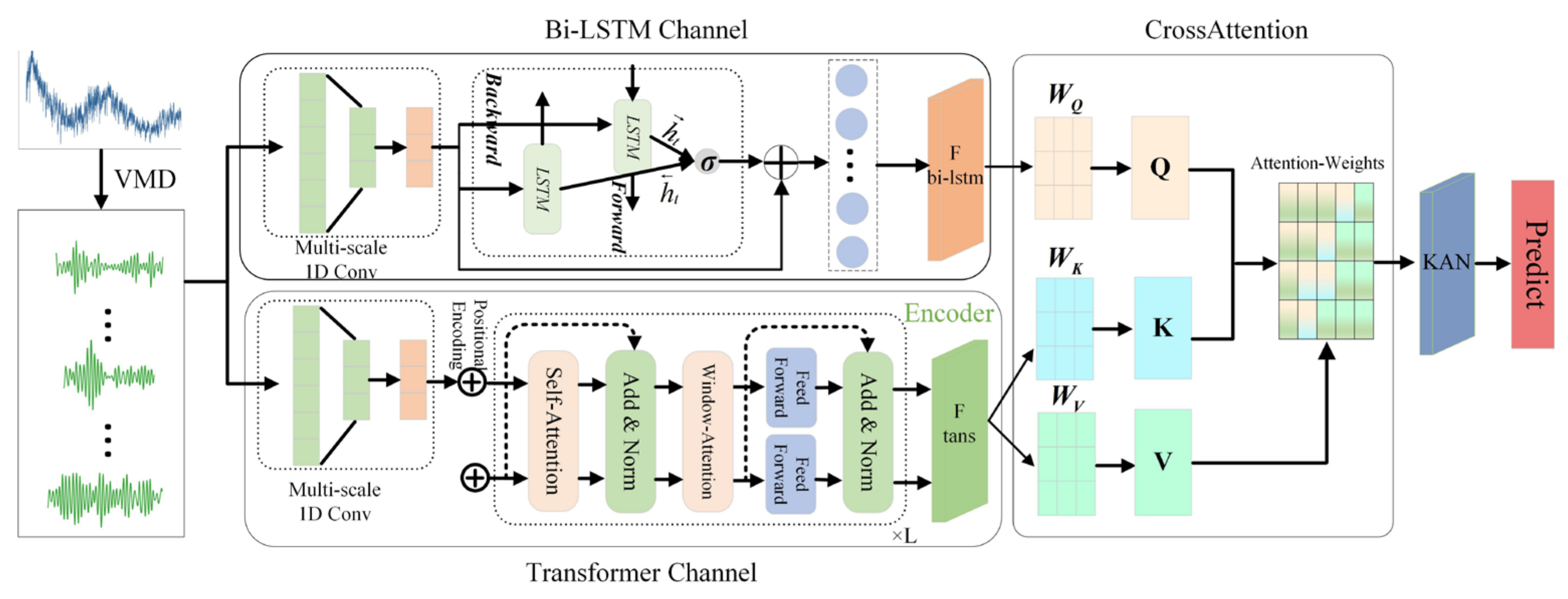
Consider the multivariate time series data $X=\left(X^{\left(1\right)}, X^{\left(2\right)}{,\dots ,X}^{\left(n\right)}\right)\in {\mathbb{R}}^{n\times T}$, where n represents the dimensionality of the multivariate time series, and T denotes the length of the time window. The i-th multivariate time series data $X^{\left(i\right)}$ is denoted as $X^{\left(i\right)}=\left(X_1^{\left(i\right)}, X_2^{\left(i\right)},\dots ,X_T^{\left(i\right)}\right)\in {\mathbb{R}}^T$, where the length of $X^{\left(i\right)}$ is T. The target time series is defined as $Y=\left(y_1,y_2 ,\dots ,y_T\right)\in {\mathbb{R}}^T$, and the length is still T. Given the original multivariate time series data $X^{\left(i\right)}=\left(X_1^{\left(i\right)}, X_2^{\left(i\right)},\dots ,X_T^{\left(i\right)}\right)$ and the target series $Y=\left(y_1,y_2 ,\dots ,y_T\right)$, our target is to predict $\widehat{Y}=\left({\widehat{y}}_{T+1},{\widehat{y}}_{T+2},\dots ,{\widehat{y}}_{T+\tau }\right)\in {\mathbb{R}}^{\tau }$, where τ denotes the forecasting horizon, and this process can be formally represented by the following Equation (1):

$${\widehat{y}}_{T+1},{\widehat{y}}_{T+2},\dots ,{\widehat{y}}_{T+\tau }=F\left(X_1,X_2,\dots ,X_T,Y\right)$$

(1)

where $F\left(·\right)$ is the nonlinear mapping we aim to learn.

3.2. VBTCKN Model

This section begins with an overview of the VBTCKN architecture; then we introduce the various components employed by the model, including the theoretical foundation of variational mode decomposition, the basic architectures of the BiLSTM model, and those of the transformer encoder model; and then we elaborate on the cross-attention mechanism and KAN networks. Finally, a comprehensive explanation of the VBTCKN is provided.

Given the complexity of time series forecasting tasks, our proposed VBTCKN model integrates multiple key components, including variational mode decomposition (VMD), bidirectional long short-term memory (BiLSTM), transformer encoder, cross-attention mechanism, and Kolmogorov–Arnold networks (KAN). Each component serves distinct purposes, shown as follows: VMD eliminates noise from time series data, the transformer encoder extracts global signals, and BiLSTM effectively captures short-term temporal dependencies. To streamline the model and accelerate computation, we retain only the encoder portion of the transformer architecture, incorporating a windowed attention mechanism within it. Preceding both the BiLSTM and transformer channels, multi-scale 1D convolutional layers are added; this design enables the rapid extraction of local features through convolutional operations, effectively reducing computational complexity while preserving rich feature representation capabilities. Furthermore, temporal dependency features extracted by BiLSTM and global dependency features are dynamically fused using an enhanced cross-attention mechanism. The incorporation of Kolmogorov–Arnold networks (KAN) allows the model to better identify temporal dynamics and nonlinear correlations in time series data, resulting in better forecasts. Figure 1 presents the structure of the proposed hybrid network, VBTCKN.

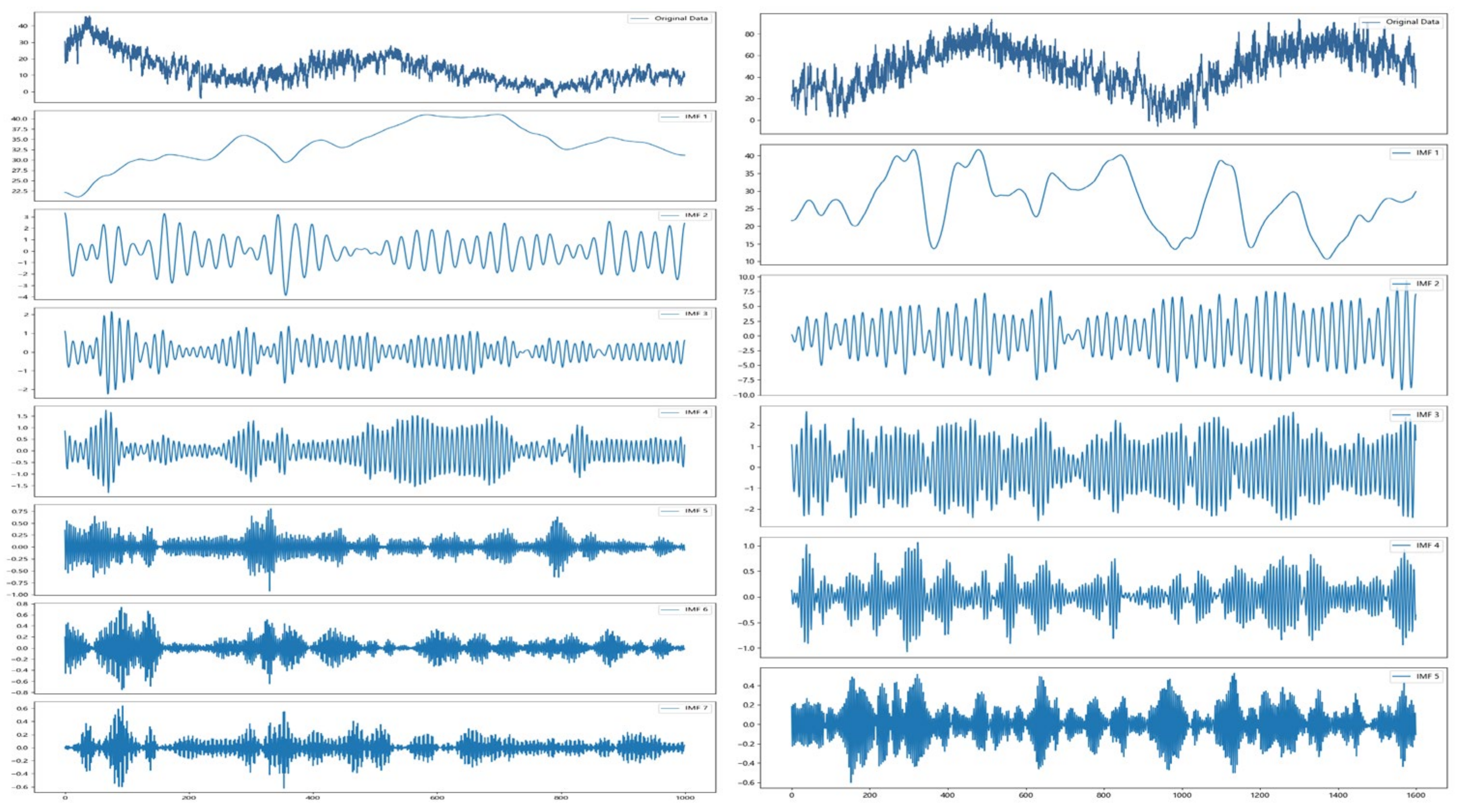
3.2.1. Variational Mode Decomposition

First introduced by Dragomiretskiy in 2013, variational mode decomposition (VMD) [30] is a signal processing method characterized by its adaptiveness and non-recursive structure. It accurately decomposes complex signals into a collection of intrinsic mode functions (IMFs) to facilitate feature extraction and analysis. Compared with alternative decomposition methods, VMD offers configurable mode quantity determination and a rigorous theoretical framework [31], effectively mitigating non-stationary characteristics in highly complex nonlinear time series.

In order to obtain specific frequencies and bandwidths for each modal function after VMD decomposition, the original signal $f\left(t\right)$ undergoes decomposition into multiple intrinsic mode functions (IMFs), and these modal functions are denoted by $u_i\left(t\right)$, where i = 1, 2, ..., K. The equation is shown as follows:

$$\begin{array}{c}min\\ \left\{{\mu }_i\right\}\left\{{\omega }_i\right\}\end{array}\left\{{\sum }_{i=1}^K{‖{\partial }_t\left[\left(\delta \left(t\right)+{\displaystyle \frac{j}{\pi t}}\right)\ast u_i\left(t\right)\right]e^{-j{\omega }_{i}t}‖}_2^2\right\}$$

(2)

$$s.t.{\sum }_{i=1}^K{u}_i\left(t\right)=f\left(t\right)$$

where $K$ is the total number of $IMFs$, $u_{kt}$ indicates the set of the $IMF$, $w_i$ signifies the center frequency set of the i-th mode, ${\delta }_t$ denotes the Dirac function, and ∗ indicates the convolution operation. To address this issue, the problem can be transformed into an unconstrained optimization formulation using the augmented Lagrangian method as follows:

$$L\left(\left\{u_i\right\},\left\{{\omega }_i\right\},\lambda \right)=\alpha {\sum }_{i=1}^K{‖{\partial }_t\left[\left(\delta \left(t\right)+{\displaystyle \frac{j}{\pi t}}\right)\ast u_i\left(t\right)\right]e^{-j{\omega }_{i}t}‖}_2^2$$

(3)

$$+‖f\left(t\right)-{\sum }_{i=1}^K{u}_i\left(t\right)‖+⟨{\lambda }_{\left(t\right)},f\left(t\right)-{\sum }_{i=1}^K{u}_i\left(t\right)⟩$$

where $\lambda$ represents the Lagrange multiplier, and $\alpha$ denotes the quadratic penalty term. The values of $\left\{u_i\right\}$ and $\left\{{\omega }_i\right\}$ can be derived through the Alternating Direction Method of Multipliers (ADMM).

To demonstrate the processing capability of variational mode decomposition in complex time series, we randomly selected the ETTh1 and GEFCom2014-E datasets from those used in this study, decomposing and visualizing their respective target time series. The ETTh1 dataset features date information and six load characteristics that collectively influence the target variable (oil temperature) through fluctuations at different frequencies, while the GEFCom2014-E dataset directly employs hourly-level load variations to affect the target oil temperature. As shown in Figure 2, VMD decomposes the target sequences of ETTh1 and GEFCom2014-E datasets into 7 and 5 subsequences, respectively, effectively reconstructing low-frequency trends, medium-frequency fluctuations, and high-frequency perturbations. This frequency–domain decomposition effectively suppresses noise interference while enhancing sequence stationarity, demonstrating VMD’s decoupling efficacy for complex temporal features. Consequently, the proposed method applies VMD to decompose the target time series, thereby mitigating noise interference in forecasting.

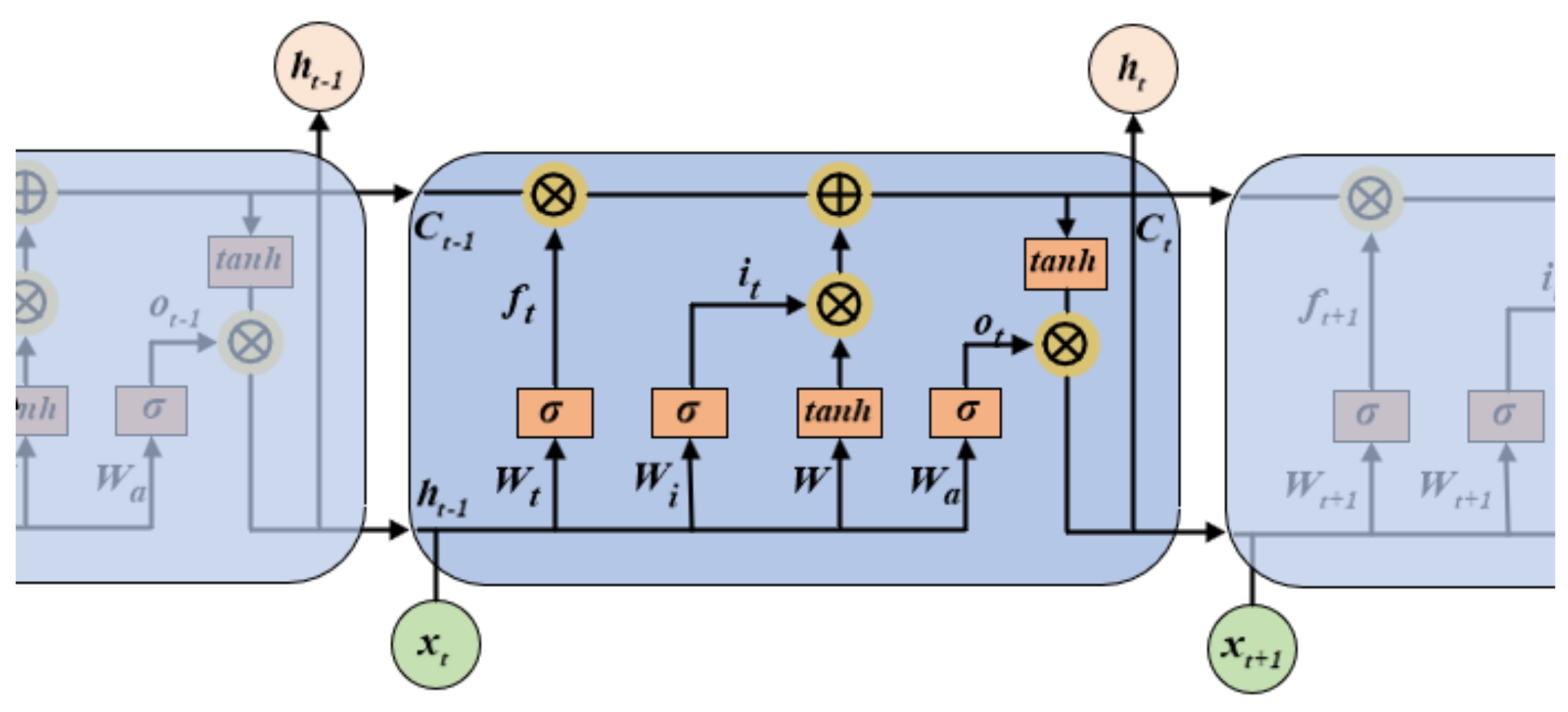
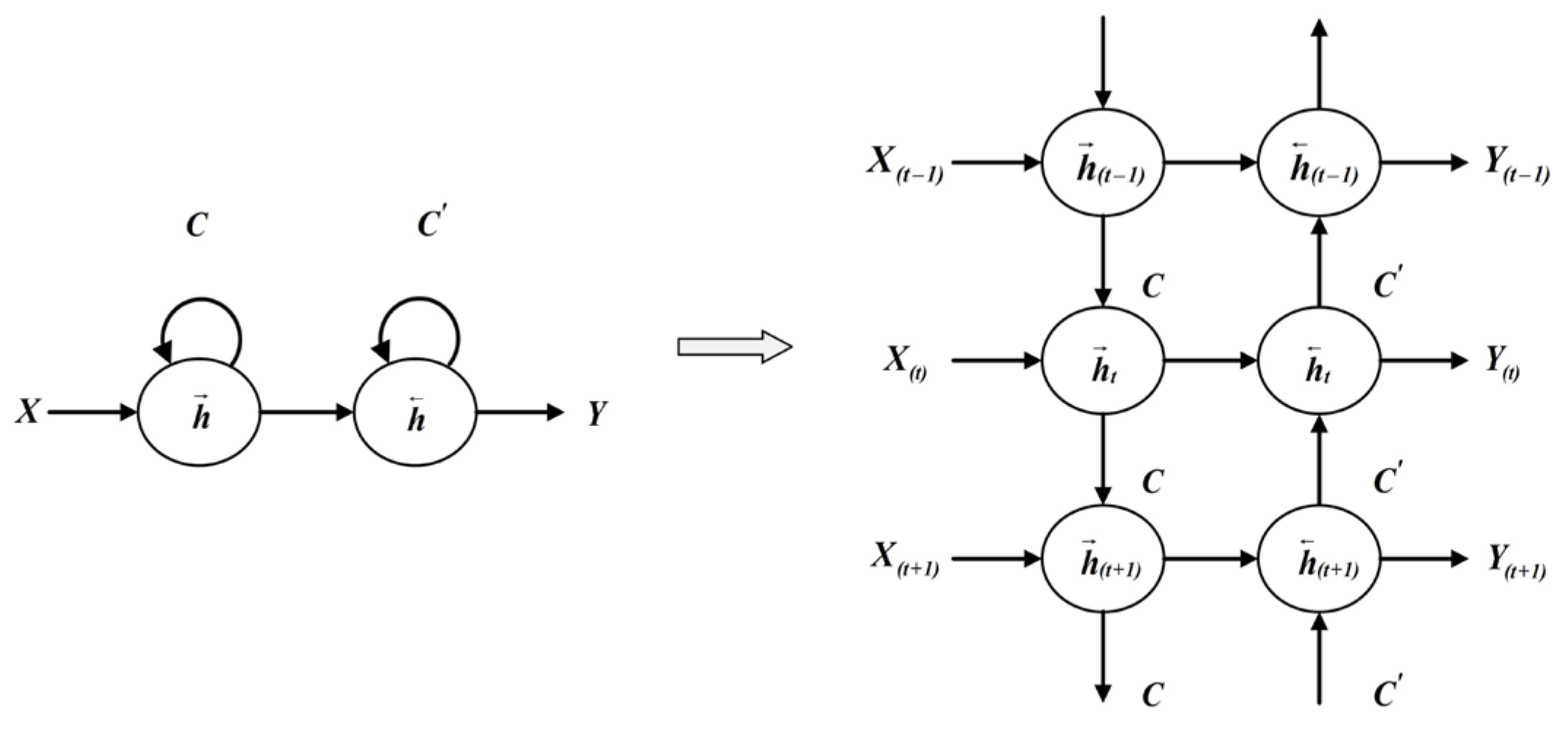
3.2.2. Bidirectional Long Short-Term Memory Network (BiLSTM)

Long short-term memory (LSTM), an enhanced architecture of recurrent neural networks (RNNs), alleviates the issues of vanishing and exploding gradients in traditional RNNs by incorporating gating mechanisms [32]. This architecture overcomes short-term memory constraints caused by sequential chain rules during backpropagation in deep RNNs, enabling the long-term selective retention of state information.

The essence of LSTM lies in its gating mechanism, which is responsible for achieving critical state control and information transmission. The forget gate filters out redundant information, the input gate controls how new data enters the cell state, and the output gate shapes the expression of state information. This functional architecture endows LSTM with superior long-term dependency capturing capacity, making it particularly suitable for addressing time-delayed phenomena in time series forecasting. Figure 3 illustrates its architecture [33].

Bidirectional long short-term memory networks (BiLSTM) represent an enhancement over LSTM, effectively processing sequential data and capturing complex dependencies between sequences with accelerated learning speed compared to unidirectional LSTMs. Bidirectional long short-term memory networks (BiLSTM) achieve the bidirectional temporal modeling of sequential data by integrating forward and backward recurrent components. Its structure comprises an input gate, an output gate, and a forget gate, each utilizing the sigmoid function to regulate information filtering and output, while integrating the tanh function to coordinate new information injection. This design circumvents the temporal constraints of unidirectional LSTM by synchronously analyzing contextual features from both directions to generate prediction outputs at time step “t”. Within each hidden layer node of BiLSTM, the following two distinct memory zones are established: one preserving historical information and the other retaining prospective information, thereby enabling the efficient storage and processing of bidirectional data flows [34]. The folded and unfolded topologies of the BiLSTM architecture are illustrated in Figure 4.

Bidirectional long short-term memory networks (BiLSTM) capture past and future input information simultaneously during time series analysis through layered stacking, enabling bidirectional data flow. Crucially, forward and backward state outputs remain logically independent, meaning weight updates for input layer and output layer neurons occur asynchronously. During forward propagation, forward and backward state information first propagates to the output layer; during backpropagation, this information passes backward via output layer neurons. Consequently, BiLSTM computes forward hidden sequences initially, subsequently processes backward hidden sequences, and finally integrates bidirectional sequences to generate outputs. This methodology fully capitalizes on contextual sequence information, providing optimized learning pathways for complex sequential patterns.

The input layer is denoted as ‘x’, the output layer as ‘y’, the hidden state as ‘h’, the bias as ‘b ‘, the weight matrix as ‘w’, the forward cell state as ‘C’, the backward state as ‘C’’, the activation function as ‘H’, and the time step as ‘t’.

The forward propagation hidden layer vector sequence is expressed as follows in Equation (4):

$$\overrightarrow{h_t}=H(w_{x\overrightarrow{h}}{x}_t+w_{\overrightarrow{h}\overrightarrow{h}}{\overrightarrow{h}}_{t-1}+b_{\overrightarrow{h}})$$

(4)

The backpropagation hidden layer vector sequence is expressed as follows in Equation (5):

$$\overleftarrow{h_t}=H(w_{x\overleftarrow{h}}{x}_t+w_{\overleftarrow{h}\overleftarrow{h}}{\overleftarrow{h}}_{t-1}+b_{\overleftarrow{h}})$$

(5)

Ultimately, the forward and backward hidden states are concatenated into an output sequence, as defined in the following formula (6):

$$h_t=w_{\overrightarrow{h}y}\overrightarrow{h_t}+w_{\overleftarrow{h}y}{\overleftarrow{h}}_t+b_y$$

(6)

In this paper, we enhance the modeling capability of time series based on BiLSTM to capture the dependencies hidden in long and complex nonlinear time series, which complement the local and global patterns extracted by the transformer channel to comprehensively capture the characteristics of time series.

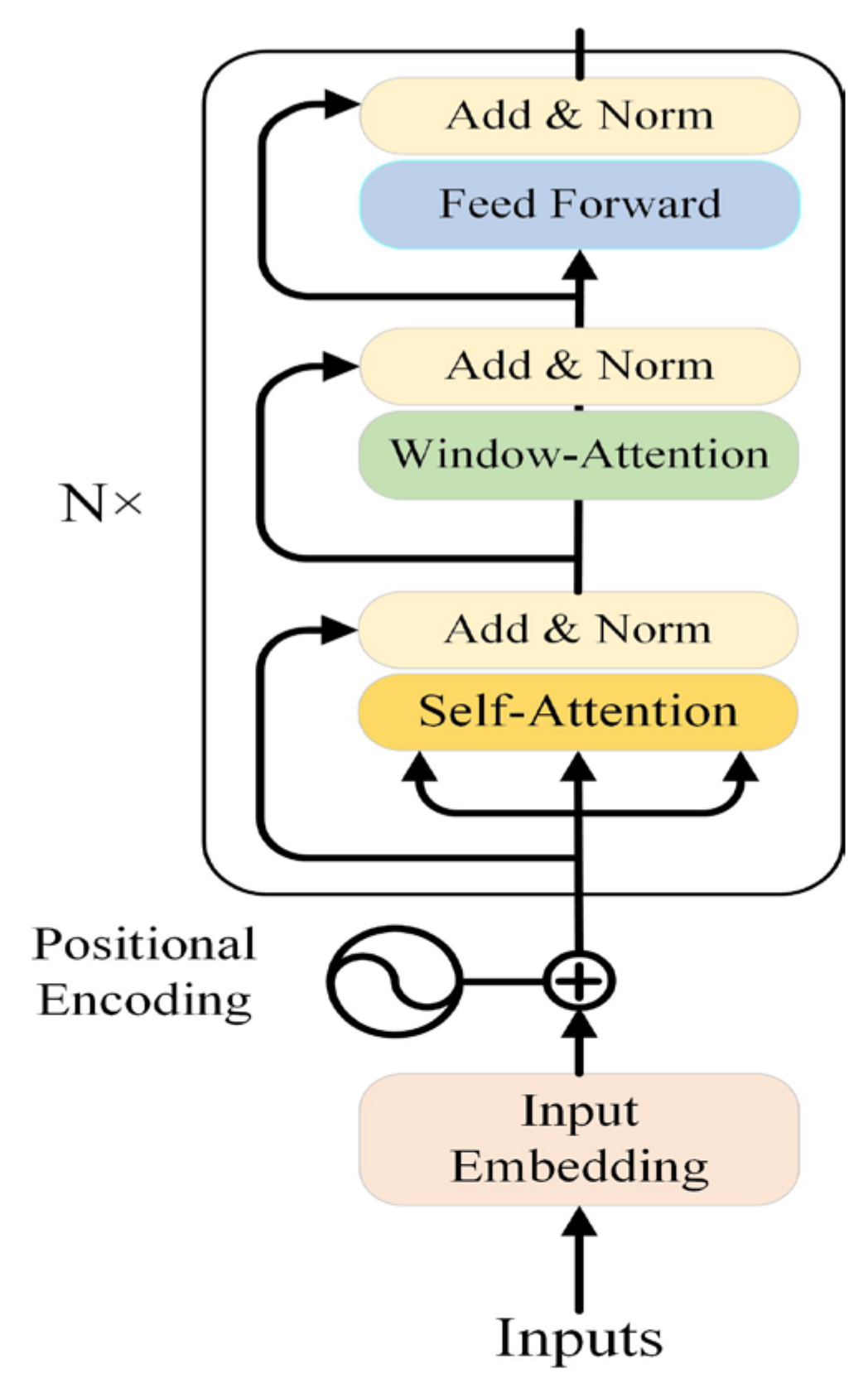
3.2.3. Transformer-Only Encoder

In contemporary machine learning, transformer models leverage their unique self-attention mechanism to gain the profound comprehension of contextual information. This architecture effectively captures local patterns and global dependencies, thus exhibiting heightened efficiency and accuracy when processing time series data [35].

The transformer encoder model, as a variant of the transformer architecture, eliminates the decoder module, enabling specific performance optimizations beyond the original transformer. The core advantage of encoder-only models lies in the dual-pronged benefits derived from their streamlined architecture. By eliminating the decoder, model parameters are substantially reduced, accommodating computation-resource-constrained scenarios; simultaneously, interpretability is enhanced as the linear data flow provides transparent computational pathways when capturing temporal dynamics and global dependencies, thus achieving heightened forecasting precision and stability. Furthermore, the sliding window attention mechanism effectively captures local information in time series forecasting, drawing inspiration from the hierarchical vision transformer proposed by Pinasthika et al. [36]. When capturing dependencies, it constrains attention calculations to fixed-size windows, computing similarity exclusively within each window and normalizing attention scores to generate weights. This approach reduces computational overhead while efficiently capturing local relationships. The architecture of the encoder-only transformer model employed in this study is illustrated in Figure 5.

The proposed approach leverages an enhanced transformer encoder architecture to integrate the strengths of temporal feature utilization and contextual information incorporation. By fully exploiting both self-attention mechanisms and sliding-window attention mechanisms, this framework efficiently extracts short-term fluctuations and global dependencies within time series data while precisely identifying complex inter-step relationships across diverse time points. This significantly advances temporal pattern comprehension and modeling capabilities. Specifically, the transformer channel focuses on extracting local patterns and global characteristics, while the BiLSTM channel captures long-range dependencies in a complementary manner. These dual channels holistically characterize complex time series properties, thereby enhancing accuracy in short-term forecasting.

3.2.4. Cross-Attention Based Fusion Methods

A cross-attention mechanism constitutes a specialized attention architecture that empowers models to concurrently attend to features in the current sequence while effectively associating and integrating information from supplementary sequences. By computing attention weights between distinct sequences, the model dynamically concentrates on relevant input characteristics during processing, thereby augmenting the comprehension of complex data structures [37].

In time series forecasting, the cross-attention mechanism effectively integrates information from multiple temporal sequences or distinct feature sources, enabling the model to autonomously capture inter-sequence dependencies and dynamically adjust its attention allocation based on contextual cues.

This paper proposes an optimized cross-attention mechanism that utilizes features extracted by the BiLSTM and transformer channels as queries, respectively, to calculate weight matrices. Through a gating mechanism, the model dynamically synthesizes these dual weight matrices, achieving the effective integration of cross-channel features. This approach fully capitalizes on the comparative strengths of both channels in capturing temporal dependencies, enabling the model to simultaneously focus on local fluctuations and global patterns within the time series. Consequently, it enhances the comprehensiveness and expressiveness of feature representation while improving precision and stability in short-term forecasting. The architecture of the cross-attention model employed in this study is shown in Figure 6.

As can be seen in Figure 6, two different input sequences $X_1$ and $X_2$ are interacted by the cross-attention mechanism to obtain the aggregated sequence $X$, allowing the model to integrate data from different sources. The model obtains data using the following equations:

$$\begin{gathered} Q_1=X_2{W}_{Q_1}{K}_1=X_1{W}_{K_1}{V}_1=X_1{W}_{V_1} \\ {Q}_2=X_1{W}_{Q_2}{K}_2=X_2{W}_{K_2}{V}_2=X_2{W}_{V_2} \end{gathered}$$

(7)

$$Z_1=softmax\left({\displaystyle \frac{Q_1{K_1}^T}{\sqrt{d_k}}}\right)V_1 Z_2=softmax\left({\displaystyle \frac{Q_2{K_2}^T}{\sqrt{d_k}}}\right)V_2$$

(8)

$$\begin{gathered} gates=Softmax\left(Linear\left(Z_1,Z_2\right)\right) \\ Z=gat{e}_1\cdot Z_1+gat{e}_2\cdot Z_2 \end{gathered}$$

(9)

where $W_Q$, $W_K$, and $W_V$ denote the trainable weight matrices, $d_k$ is the dimensions of keys and queries in the attention mechanism, Z₁ and Z₂ are the intermediate results generated as query vectors for different input sequences X₁ and X₂, respectively, gates are the generated gating weights, gate₁ is gates[:,:,0] for the first weight coefficients, gate₂ is gates[:,:,1] for the second weight coefficients, and Z is the final feature fusion representation. Softmax is employed to normalize attention scores into a probabilistic format, allowing the model to adaptively attend to distinct portions of the input sequence.

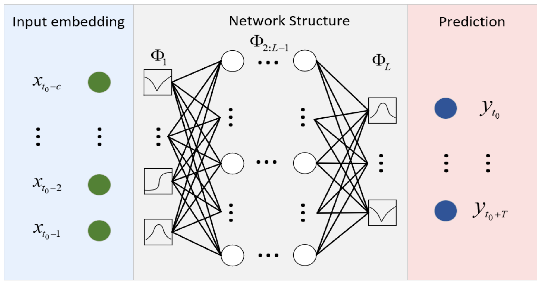
3.2.5. Kolmogorov–Arnold Networks (KAN)

Kolmogorov–Arnold networks (KAN), introduced by Liu et al. [38] in 2024 as a novel deep learning architecture, specialize in efficiently learning complex mapping relationships. As a contemporary alternative to traditional multi-layer perceptrons (MLP), Kolmogorov–Arnold networks (KAN) embody Kolmogorov’s representation theorem and Arnold’s dynamic system principles through their hierarchical architecture and adaptive activation functions. This design enables the more effective capture of nonlinear characteristics within data, consequently enhancing machine learning models’ performance in high-dimensional data processing.

Similar to multi-layer perceptrons (MLP), KAN employs a fully connected structure, yet innovatively transitions nonlinear functionality from fixed neuron activation functions to the connection weights. Diverging from the static linear weights in MLPs, KAN characterizes the weight parameters by employing trainable 1D spline functions. KAN nodes solely perform the additive aggregation of input signals, while all nonlinear transformations are executed through spline functions applied to weights. This architecture enables the flexible modeling of complex nonlinear relationships via the dynamic refinement of spline functions, concurrently reducing reliance on conventional activation mechanisms.

Leveraging its hierarchical architecture and adaptive activation functions, KAN effectively captures nonlinear data characteristics and models complex interactions while diminishing reliance on conventional activation mechanisms. However, given their unique architecture and complex mappings, they exhibit suboptimal interpretability and elevated computational costs arising from hierarchical mappings and spline function calculations [39]. In light of these limitations, this paper employs VMD to preprocess time series for complexity reduction while simultaneously decreasing the network depth to alleviate computational pressure on KAN. Figure 7 illustrates the structural framework of KAN [40].

This paper employs KAN networks to enhance model flexibility and expressive capacity. The feature vector fused via the cross-attention mechanism—drawn from BiLSTM and transformer outputs—is input into the KAN network {$x_{t_0-c:t_0-1}$} and then processed through KAN to generate prediction results {$y_{t_0:T}$}. The KAN network further enhances deep feature representations following cross-attention fusion, enabling the more effective modeling of complex nonlinear sequences. The computational formula is shown as follows:

$$\mathrm{y}=\mathrm{KAN}\left(x\right)=({\Phi }_L\circ {\Phi }_{L-1}\circ \dots \circ {\Phi }_1)\left(x\right)$$

(10)

where KAN contains L layers, and the matrix $\Phi$ denotes the nonlinear mapping. Each layer of ${\Phi }_l$ is a nonlinear transformation consisting of a matrix and a set of trainable univariate spline functions (${\varphi }_{i,j}$), and the different layers are connected by the composite operation $\circ$ to form a hierarchical mapping relation.

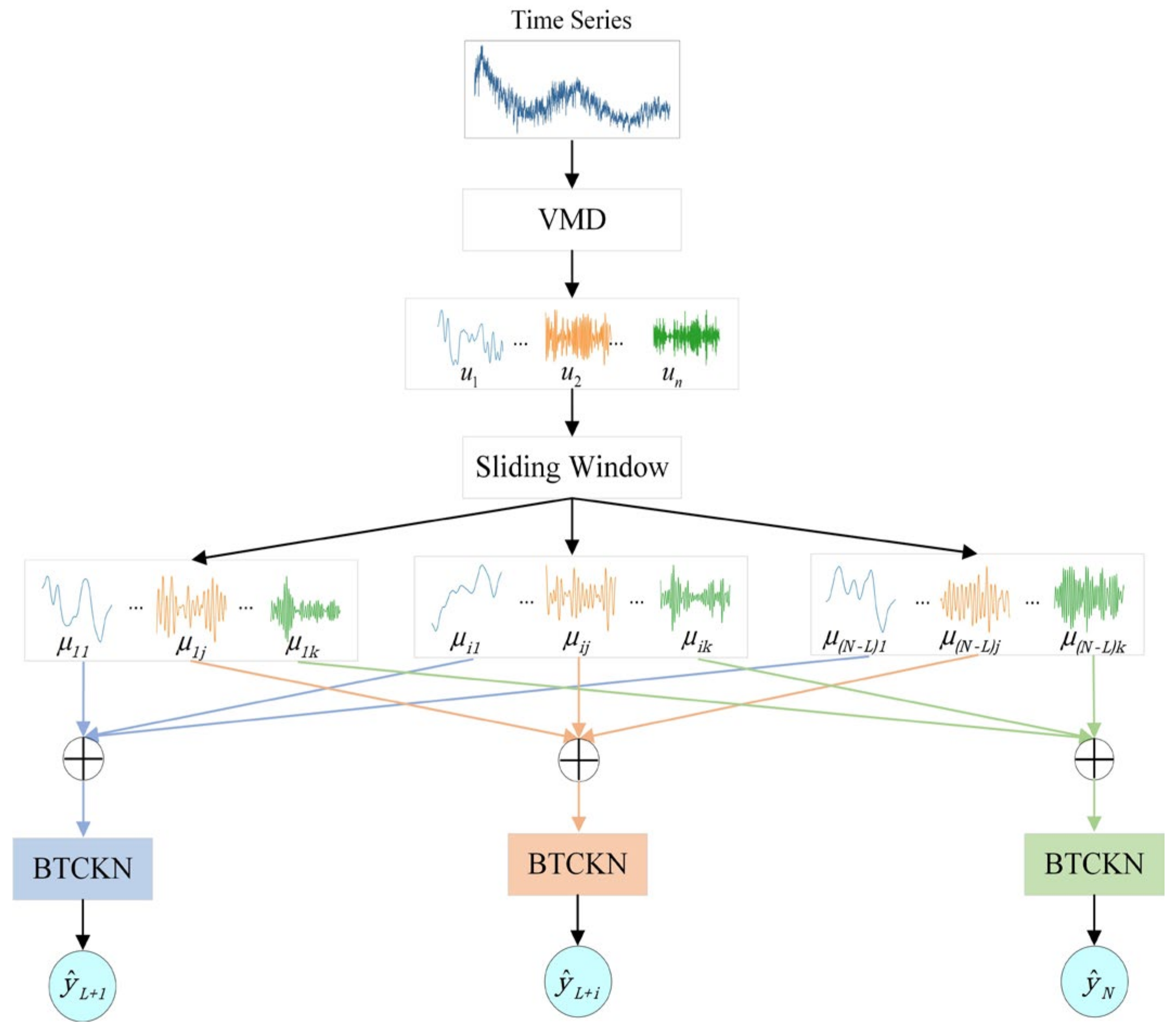
3.2.6. VBTCKN Model Prediction Process

To improve the accuracy of short-term time series forecasting by mitigating sequence variability and volatility, we introduce a novel approach that integrates variational mode decomposition (VMD) with a dual-channel cross-attention network. As illustrated in the model flowchart (Figure 8), the workflow begins with applying VMD to decompose the original time series into multiple frequency-complementary modal components, utilizing symmetric frequency distribution constraints to reduce sequence fluctuations. After decomposition, the modal components are partitioned into sub-windows via sliding windows to facilitate the extraction of local temporal dynamics. These sub-windows undergo aggregation before being fed into two parallel channels; the BiLSTM channel extracts short-term dependencies, while the transformer channel captures global dependency relationships. The resulting features are integrated through cross-attention for fusion and are subsequently processed by KAN networks to generate predictions, abbreviated as BTCKN in the diagram. During backpropagation, the dual-channel attention network calculates channel-specific adaptive weights to ensure complementary interaction between both pathways, thereby enhancing model robustness and generalization capabilities.

• VMD and Sliding Window

The left side of Figure 1 illustrates the processing methodology for the input time-series $X$ = {$x_1, { x}_2, \dots ,x_t$}, where the target value corresponding to the i-th column is denoted as $X_i$. The original time series {$u_1$, $u_2$, …, $u_K$} is first decomposed into K modal subsequences by variable mode decomposition (VMD), based on Equation (1), where each subsequence represents a different frequency component. The resulting modal subsequence is then input into a sliding window, and a sliding window operation is performed on each decomposed modal subsequence $u_j$. In each subsequence, a set of sub-windows is generated through the sliding window, as follows:

$$\begin{gathered} W_{1,j}=\left\{u_{1,j},u_{2,j},\dots ,u_{L,j}\right\} \\ {W}_{2,j}=\left\{u_{2,j},u_{3,j},\dots ,u_{L+1,j}\right\} \\ {W}_{N-L+1,j}=\left\{u_{N-L+1,j},\dots ,u_{N,j}\right\} \end{gathered}$$

(11)

where the window size is L. The above sliding window operation satisfies the following relationship:

$${\sum }_{i=1}^K{u}_{ij}=W_i$$

(12)

The sliding window results for each modal subsequence are then combined by position to form the complete input $W=\left\{W_1,W_2,\dots ,W_{N-L+1}\right\}$. This allows the data to be predicted by the following formula:

$$\begin{gathered} {\widehat{y}}_{i+L}=F\left(W_i\right) \\ =\mathrm{F}\left(x_{i,}{x}_{i+1},\dots ,x_{i-L+1}\right) \end{gathered}$$

(13)

where F(⋅) is the VBTCKN model of this paper.

2.

BiLSTM Channel

As shown in the upper part of Figure 1, the BiLSTM channel for extracting short-term dependencies consists of a multiscale one-dimensional convolutional layer, BiLSTM layers, residual connections, and a fully connected module. For the three-dimensional vector $X$ = {$x_1, { x}_2, \dots ,x_t$} processed by VMD and the sliding window, it is input into the BiLSTM channel to extract the features, and the process is as follows.

First the multi-scale 1D convolutional layer performs feature extraction on the input sequence according to different convolutional kernel sizes to generate more representational local features, and the convolution is computed as shown below:

$$X_{conv}=W\ast X+b \mathrm{where} X_{conv}\in {\mathbb{R}}^{N\times T^{\prime }\text{×}\mathrm{d}}$$

(14)

where the convolved timestep count is given by T′ = T − k + 1, and d represents the number of convolution kernels, while W and b denote their weight parameters and bias terms, respectively. The refined temporal features $X_{conv}$ are processed by the BiLSTM to capture short-term dependencies within the time series, as shown in the following Equation (15):

$$h_t=BiLSTM\left(X_{conv}\right)$$

(15)

where $h_t$ represents the feature vector extracted by BiLSTM at moment t, which is computed in Equations (4)–(6). Subsequently, the BiLSTM output features $h_t$ are summed with the original inputs $X_t$ to obtain the output features after residual concatenation, as shown in the following Equation (16):

$$h_t^{\prime }=h_t+X_t$$

(16)

where $h_t^{\prime }$ denotes the output features after adding the residuals. The residual-connected feature $h_t^{\prime }$ is then passed to the fully connected module for further nonlinear mapping to extract richer features.

3.

Transformer Channel

As shown in the lower part of Figure 1, the primary objective of constructing the transformer channel is to identify multi-scale characteristics and local dependencies within time series data. This part consists of a multi-scale one-dimensional convolutional modeling layer, a transformer encoder part, and a fully connected layer. Firstly, the three-dimensional vector $X$ = {$x_1, { x}_2, \dots ,x_t$}, which has been processed by the VMD and the sliding window, is input into the multiscale 1D Conv to extract the local features, where the convolution operation is shown in Equation (14).

Then, the extracted local features $X_{conv}$ are input into the transformer encoder, which leverages self-attention and windowed attention mechanisms to model the global and local temporal characteristics of the time series. The computational procedure for the self-attention mechanism is shown as follows:

$$Q_t=X_{conv}{W}_Q^{\prime }{K}_t=X_{conv}{W}_K^{\prime }{V}_t=X_{conv}{W}_V^{\prime }$$

(17)

$$A\mathrm{ttention}(\mathrm{Q},\mathrm{K},\mathrm{V})=\mathrm{s}\mathrm{o}\mathrm{f}\mathrm{t}\mathrm{m}\mathrm{a}\mathrm{x}\left({\displaystyle \frac{Q_t{K_t}^T}{\sqrt{d_k^{\prime }}}}\right)V_t$$

(18)

where $W_Q^{\prime }$, $W_K^{\prime }$, and $W_V^{\prime }$ denote the trainable weight matrices, $d_k^{\prime }$ refers to the dimensionality of both the key and query vectors in the attention mechanism, and it serves to normalize the dot product, thereby avoiding disproportionately large outputs. The Softmax function operates by converting the input vector into probability distributions, thereby obtaining the attention weights. The computed attention results are further normalized hierarchically by the following equation:

$$Z_{self}=LayerNorm\left(A\mathrm{ttention}\right(\mathrm{Q},\mathrm{K},\mathrm{V})+X_{conv})$$

(19)

Subsequently, the window attention mechanism processes the input to extract localized feature representations. It reshapes the input Z_self into a sequence of features Z_w with a window size w by dividing the input into non-overlapping windows, and then, it performs the computation as described in Equations (17)–(19) to obtain the window attention output Z. The computed attention result is further subjected to nonlinear activation ReLu and hierarchical normalization LayerNorm as follows:

$$FFN\left(Z\right)=ReLU(Z{W}_1+b_1)W_2+b_2$$

(20)

$$H=LayerNorm\left(FFN\right(Z)+Z)$$

(21)

where $W_1$ and $W_2$ denote the trainable weight matrices, with $b_1$ and $b_2$ serving as their respective biases. The feature vector H obtained by the transformer encoder is passed to the fully connected module for further nonlinear mapping to extract richer features.

4.

The predict of the model

The features extracted from the BiLSTM channel and transformer channel, respectively, are fused by an improved cross-attention mechanism to capture the interconnections between different feature channels. In the cross-attention mechanism, firstly, the output of the BiLSTM channel is used as query and the output of the transformer channel is used as key and value, and the fused feature representations are obtained by cross-attention computation $Z_{corss1}$. Then, the output of the transformer channel as query and the output of the BiLSTM channel as key and value are used to obtain the fused feature representation $Z_{c\mathrm{ro}ss2}$; the feature fusion of $Z_{c\mathrm{ro}ss1}$ and $Z_{c\mathrm{ro}ss2}$ is realized through a dynamic gating mechanism, which is calculated in Equations (7)–(9). This fusion not only integrates the local and global features in the time series, but it also enhances the complementarity of the features of different channels to form a more comprehensive characterization of the target.

Then, it is inputted into the KAN network for nonlinear mapping for the further high-dimensional processing of the features, and it finally generates the prediction results at moment t. The role of the KAN network is to utilize the fused deep features to flexibly model complex nonlinear relationships, thus improving the accuracy of the prediction. Its computational process can be expressed as follows:

$$y_t=KAN\left(Z_{cross}\right)$$

(22)

where $y_t$ denotes the final prediction result at moment t, and $Z_{cross}$ is the feature representation after cross-attention fusion. Algorithm 1 describes the overall process.

Algorithm 1 VBTCKN

Input: Time-series X = (X1, X2, X3, ..., Xt), Time-step L, Train-epoch n, vmd_params(K, α, τ), kernel_size k Output: Predict time-series Y = (Yt+1, Yt+2, Yt+3, ...,Yt+L), mean absolute error MAE, mean squared error MSE, root mean square error RMSE, Coefficient of Determination R2

1 X = vmd_decomposition (X, α, τ, K) 2 for t to n do: 3 for i to L do: 4  for j to L do: 5   bilstm channel calculate encoding vector hb←Xi 6    for s in k do: 7     Xs = conv1d = W × Xi + b 8    Xconv = concat(Xs) 9    ${\overrightarrow{h}}_b=H\left(w_{x\overrightarrow{h}}{x}_{\mathrm{conv}}+w_{\overrightarrow{h}\overrightarrow{h}}{\overrightarrow{h}}_{i-1}+{ b}_{\overrightarrow{h}}\right)$ 10    ${\overleftarrow{h}}_b=H\left(w_{x\overleftarrow{h}}{x}_{\mathrm{conv}}+{ w}_{\overleftarrow{h}\overleftarrow{h}}{\overleftarrow{h}}_{i-1}+b_{\overleftarrow{h}}\right)$ 11    $h_b=w_{\overrightarrow{h}y}{\overrightarrow{h}}_b+{ w}_{\overleftarrow{h}y}{\overleftarrow{h}}_b+b_y$ 12    dropout layer 13    LayerNormal layer 14   transformer channel calculate encoding vector ht←Xi 15    for s in k do: 16     Xs = conv1d = W × Xi + b 17    Xconv = concat(Xs) 18    $e_{\mathrm{ij}}=$a (${X }_{\mathrm{conv}}^{i-1}, {X }_{\mathrm{conv}}^j$) 19     ${\alpha }_{\mathrm{ij}}={\displaystyle \frac{exp\left(e_{ij}\right)}{{\sum }_{k=1}^{T_x}exp\left(e_{ik}\right)}}=\mathrm{softmax}\left(e_{ij}\right)$ 20     $h_t^{\text{‘}}=\mathrm{self}\mathrm{Attention}\left(Xconv\right)=\sum _{i=1}^{T_x}{\mathsf{\alpha }}_{ij}{X }_{conv}^j$ 21     $e_{ij}=$a (${h_t^{\text{‘}}}^{i-1}, {h_t^{\text{‘}}}^j$ ) 22    ${ h}_t=\mathrm{windowAttention}\left(h_t^{\text{‘}}, \text{⌈}t/w\text{⌉}, w\right)={\sum }_{j=1}^w{\displaystyle \frac{exp\left(e_{ij}\right)}{{\sum }_{k=1}^{w}exp\left(e_{\mathrm{ik}}\right)}}{h}_t^{\text{‘}}$ 23     Feed Forward layer 24     dropout layer 25     LayerNormal layer 26    Cross-attention layer calculate decoding vector yi ←hb, ht 27     ${ Z}_1=\mathrm{softmax}\left({\displaystyle \frac{\left(h_b{W}_Q\right){\left(h_t{W}_K\right)}^T}{\sqrt{d_k}}}\right)\left(h_t{W}_V\right)$; ${ Z}_2=\mathrm{softmax}\left({\displaystyle \frac{\left(h_t{W}_Q\right){\left(h_b{W}_K\right)}^T}{\sqrt{d_k}}}\right)\left(h_b{W}_V\right)$ 28     $\mathrm{gates}=\mathrm{softmax}\left(\mathrm{Linear}\right(Z_1, Z_2\left)\right)$ 29     $Z_{cross }={gates}_1\text{·}{Z}_1+{gates}_2\text{·}{Z}_2$ 30     KAN network layer predict Y = KAN($Z_{cross}$ ) 31   end 32  end 33 end 34 calculate MAE MSE RMSE R2 35 return Y MAE MSE RMSE R2

4. Experiments

This section opens with an overview of the evaluation methodologies and performance criteria employed in assessing the model followed by a detailed exposition of data preprocessing strategies and experimental parameter configurations. Subsequently, experimental results are analyzed comprehensively, culminating in comparative experiments and ablation analysis.

4.1. Model Performance Evaluation Indicators

The assessment of model performance employs multiple prevalent error metrics, with their specific formulae and explanations given below.

• Mean absolute error

Mean absolute error (MAE), a widely used metric, calculates the average absolute deviation between predicted and observed values to reflect prediction accuracy, as follows:

$$MAE={\displaystyle \frac{1}{n}}{\sum }_{i=1}^n|y_i-{\widehat{y}}_i|$$

(23)

2.

Mean square error

The mean squared error (MSE) is a statistical metric for assessing prediction accuracy. It quantifies prediction accuracy by averaging squared prediction errors, thus reflecting the overall error magnitude, as follows:

$$MSE={\displaystyle \frac{1}{n}}{\sum }_{i=1}^n{\left(y_i-{\widehat{y}}_i\right)}^2$$

(24)

3.

Root mean square error

Root mean square error (RMSE) is a widely used metric that measures prediction accuracy as the square root of the mean squared error between actual and predicted values and is shown as follows:

$$RMSE=\sqrt{{\displaystyle \frac{1}{n}}{\sum }_{i=1}^n{\left(y_i-{\widehat{y}}_i\right)}^2}$$

(25)

4.

Coefficient of determination $R^2$

The coefficient of determination, denoted as $R^2$, serves as an indicator in regression analysis for evaluating model fit. Its value ranges between 0 and 1 inclusive, with a higher magnitude signifying enhanced explanatory power of the model over the data, and the equation is shown as follows:

$$R^2=1-{\displaystyle \frac{{\sum }_{i=1}^N(y_i-{\widehat{y}}_i{)}^2}{{\sum }_{i=1}^N(y_i-\bar{y}{)}^2}}$$

(26)

In Equations (23)–(26), $y_i$ and ${\widehat{y}}_i$ denote the true and predicted values at time step i, respectively, while $\bar{y}$ depicts the mean of the target variable, with n representing the sample size.

4.2. Datasets

This study employs the following four open-source datasets: the Electricity Transformer Temperature (ETT) dataset [41] encompassing four subsets (ETTh1, ETTh2, ETTm1, and ETTm2); the Weather dataset [41]; the Global Energy Forecasting Competition 2014—Electricity Load dataset (GEFCom2014-E) [42]; and the Solar-Energy dataset [43].

4.2.1. Electricity Transformer Temperature Dataset

The ETT (Electricity Transformer Temperature) dataset constitutes a publicly available benchmark specifically developed for time series forecasting research concerning the temperature prediction of transformers in electrical power systems. This dataset spans from July 2016 to July 2018 and contains seven categories of electrical load features. It employs six-dimensional feature vectors to predict the oil temperature (OT value) of transformers representing power consumption loads, thereby establishing a multivariate time series benchmark. This study employs the following four subsets: ETTh1 and ETTh2 (hourly), and ETTm1 and ETTm2 (15 min intervals). Recognized as a critical resource in time series forecasting, this dataset distinguishes itself through its high temporal resolution and comprehensive coverage scope.

4.2.2. Weather Dataset

The Weather dataset represents a publicly accessible benchmark specifically designed for research on future weather conditions within time series forecasting. The dataset covers the weather as well as temperature changes from January 2020 to January 2021, and it includes a total of 21 weather metrics such as air humidity, barometric pressure, temperature, precipitation, etc., to predict the changes in temperature (OT). This dataset was collected at a frequency of every 10 min with high temporal granularity.

4.2.3. GEFCom2014-E Dataset

The GEFCom2014-E dataset is a publicly available time series dataset provided by the Global Energy Forecasting Competition 2014 (GEFCom 2014) and is dedicated to the study of energy load forecasting. The dataset is a multivariate time series dataset covering temperature as well as electricity load variations from January 2006 to December 2014 with four features, which are date, hour, load, and temperature. The dataset was collected at a 1 h granularity, making it possible to more accurately capture the pattern of changes in electricity demand over time for time series forecasting.

4.2.4. Solar-Energy Dataset

The Solar-Energy dataset contains records of solar energy output in 2006 from 137 PV plants located in Alabama. Collected at a granularity of 10 min, the dataset was designed for solar power forecasting and provides high-resolution time series data suitable for studying and modeling complex time-dependent relationships.

For this experiment, we selected these datasets for experimental analysis, and

Table 1. Datasets.

Dataset Name	Data Size	Variables	Train Size	Test Size
ETTh1	17,420	8	15,678	1742
ETTh2	17,420	8	15,678	1742
ETTm1	69,680	8	62,712	6968
ETTm2	69,680	8	62,712	6968
Weather	52,696	22	47,426	5270
GEFCom2014-E	78,888	4	70,999	7889
Solar-Energy	52,560	137	23,911	2657

presents the details of the four datasets. (ETT contains four subsets).

4.3. Data Preprocessing

During dataset preprocessing, all four datasets underwent transformation into three-dimensional tensors structured in the [samples, timesteps, features] format to facilitate subsequent model training.

We conducted missing value and outlier analysis on all four datasets. Only in the Solar-Energy dataset did we identify anomalous values consisting entirely of zeros, with an outlier proportion of 0.505. To ensure prediction rationality, we removed partial data, resulting in a final dataset containing 26,568 entries. Additionally, for the Weather dataset, since features such as wind speed and wind direction showed weak correlations with the target variable (temperature), we employed a feature correlation matrix to exclude those features exhibiting correlation coefficients lower than 0.1 relative to the target value.

For all four datasets, we adopted the last column of the features as the prediction target and processed the target features with variational mode decomposition. Given the characteristics of time-series data, a 9:1 train-test split was used to enable effective model training. Following slice processing of the dataset, Min–Max normalization was applied to mitigate interference from numerical range discrepancies on experimental outcomes. To ensure the interpretability of final predictions, model outputs underwent inverse normalization to restore original data scales.

4.4. Experimental Setup

In terms of experimental settings, we set the window size to 60 and conducted experiments in 1–20 prediction time steps.

Table 2. Experimental parameter settings.

Parameter/Dataset	ETT/Solar-Energy	Weather/GEFCom2014-E
epoch	100	100
batch_size	128	128
sliding window size	60	60
kan_layer	2	2
dropout	0.3	0.3
optimizer	Adam	Adam
loss function	huber-loss	huber-loss
activation function	relu	relu
learning rate	1 × 10–3	1 × 10–3
bilstm_Layer	2	1
transformerEncoder_Layer	2	4
heads	2	8
hidden_dim	64	32

delineates the primary model parameter configurations. During training, the epoch was set to 100 and the batch_size to 128. Considering disparities in scale and sampling frequency across datasets, the BiLSTM adopted a two-layer structure with a hidden layer dimension of 64 when processing ETT and Solar-Energy data, employing ReLU activation and a convolution kernel size of 3; the transformer encoder similarly adopted a two-layer architecture featuring 2 attention heads and a 64-dimensional hidden layer. For the Weather and GEFCom2014-E datasets, we adjusted the number of BiLSTM layers to 1, the number of encoder heads for the transformer to 8, the number of layers to 4, and the number of hidden layers to 32. To mitigate overfitting, a dropout operation with a discard rate of 0.3 was applied after each LSTM module. Concurrently, batch normalization was implemented to enhance output stability across network layers. Huber Loss was adopted in training, with Adam optimization initialized at a learning rate of 0.001 and decayed by 1 × 10^–5 per epoch. Within the variational mode decomposition (VMD) framework, the sliding window size was configured as 60, the bandwidth constraint parameter was set to 2000, the noise tolerance was assigned a value of 0, and the convergence threshold was specified as 1 × 10^–7. Given the significant impact of the K value in VMD on prediction performance, it should be separately selected for each dataset. When K is excessively large, decomposition may become over-fragmented, diminishing interpretability and increasing computational load; conversely, inadequate K values lead to the insufficient resolution of decomposition, potentially causing information loss. Therefore, we conducted an experimental analysis for the value of K, as shown in

Table 3. Performance of VBTCKN at different values of K (ETTh1, ETTh2, and ETTm1).

Dataset	ETTh1				ETTh2				ETTm1
K	MAE	MSE	RMSE	R2	MAE	MSE	RMSE	R2	MAE	MSE	RMSE	R2
5	0.261	0.13	0.361	0.976	0.433	0.316	0.562	0.983	0.152	0.044	0.211	0.992
6	0.28	0.148	0.385	0.973	0.54	0.444	0.666	0.977	0.123	0.031	0.176	0.994
7	0.239	0.101	0.318	0.981	0.238	0.103	0.322	0.994	0.101	0.019	0.137	0.996
8	0.215	0.08	0.291	0.984	0.262	0.135	0.367	0.993	0.113	0.024	0.156	0.995
9	0.181	0.056	0.237	0.989	0.199	0.07	0.265	0.996	0.121	0.026	0.163	0.994
10	0.212	0.073	0.271	0.986	0.212	0.081	0.285	0.995	0.112	0.023	0.155	0.995

,

Table 4. Performance of VBTCKN at different values of K (ETTm2, Weather, and GEFCom2014-E).

Dataset	ETTm2				Weather				GEFCom2014-E
K	MAE	MSE	RMSE	R2	MAE	MSE	RMSE	R2	MAE	MSE	RMSE	R2
4	0.092	0.016	0.128	0.999	0.034	0.002	0.047	0.984	0.486	0.413	0.642	0.993
5	0.087	0.013	0.117	0.999	0.027	0.002	0.043	0.987	0.171	0.05	0.224	0.999
6	0.084	0.014	0.116	0.999	0.021	0.001	0.035	0.991	0.256	0.105	0.325	0.998
7	0.072	0.009	0.097	0.999	0.033	0.002	0.046	0.985	0.251	0.108	0.328	0.998
8	0.121	0.022	0.149	0.998	0.031	0.002	0.045	0.985	0.329	0.168	0.41	0.997

and

Table 5. Performance of VBTCKN at different values of K.

Dataset	Solar-Energy
K	MAE	MSE	RMSE	R2
10	0.228	0.089	0.298	0.999
11	0.213	0.076	0.276	0.999
12	0.164	0.045	0.213	0.999
13	0.166	0.048	0.219	0.999
14	0.229	0.082	0.287	0.998

. After the experimental analysis, we concluded that we set the K value to 9 in ETTh1 and ETTh2 datasets, 7 in ETTm1 and ETTm2, 6 and 5 in Weather and GEFCom2014-E, respectively, and 12 in Solar-Energy.

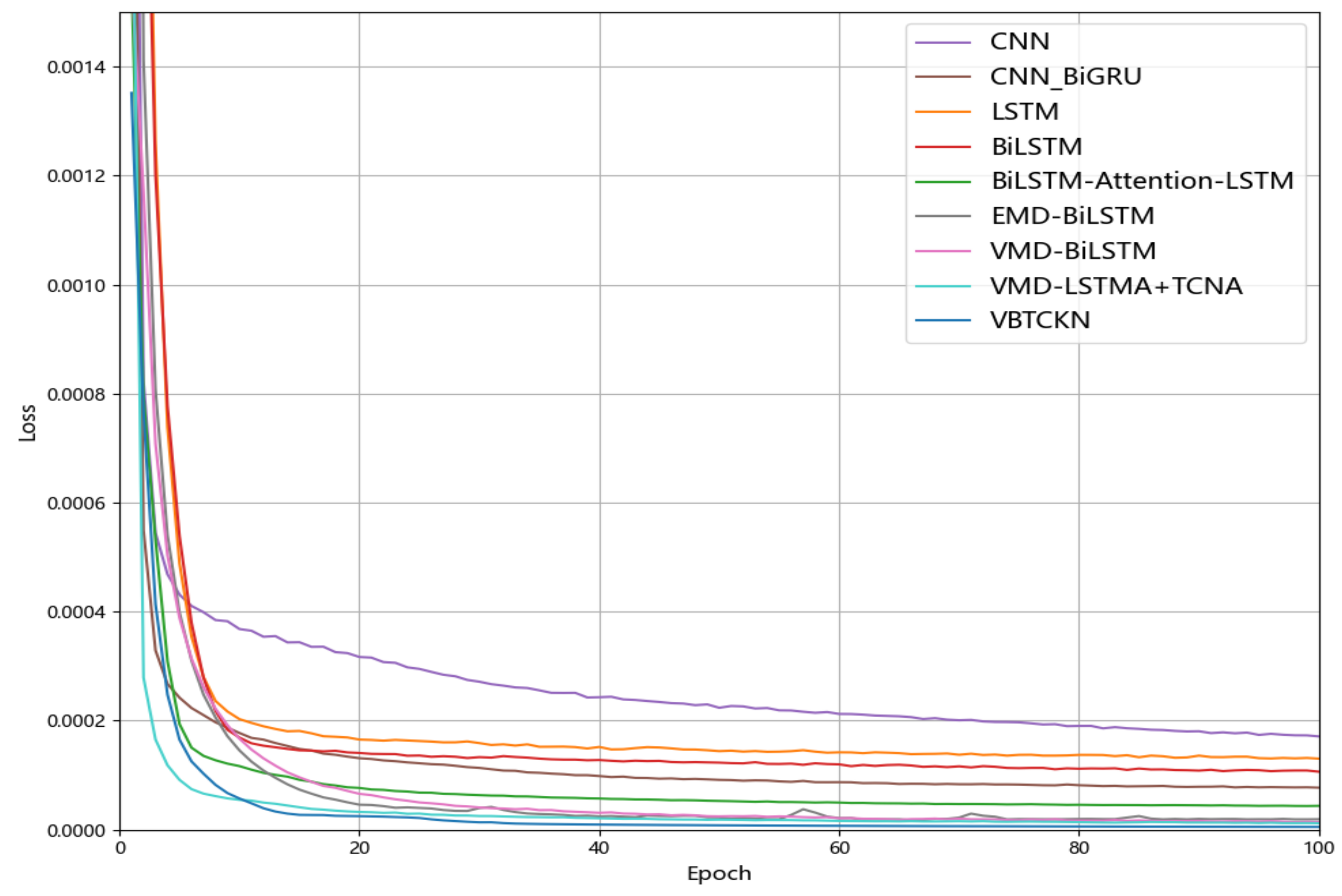
4.5. Experimental Results and Analysis

Figure 9 presents a comparative visualization of loss curves during training for the VBTCKN model against short-term time series forecasting models—CNN [18], CNN-BiGRU [44], LSTM, BiLSTM, EMD-BiLSTM [27], VMD-BiLSTM [45], BiLSTM-attention-LSTM [46], and VMD-LSTMA+TCNA [31]—on the ETTm2 dataset under a forecasting horizon of 10 steps. The figure illustrates that our model’s loss decreases quickly at the start of training and stabilizes later, remaining consistently below those of other models. This outcome reflects the model’s effective extraction of temporal features and steady convergence during training, demonstrating its solid learning ability.

Figure 10 demonstrates the predictive efficacy of the VBTCKN model on the ETTm2 dataset under a forecast horizon of 10 steps. It is observable that the model exhibited robust fitting capabilities on the test set, accurately capturing both the evolutionary trends of the raw time-series data and its local fluctuation patterns. This evidence substantiates that VBTCKN achieves balanced performance in complex temporal modeling, maintaining high prediction precision while mitigating overfitting, thereby demonstrating proficient feature extraction and dynamic restoration capabilities.

Figure 11 shows the loss plot of the VBTCKN model on top of the ETTh1, ETTh2, ETTm1, ETTm2, GEFCom2014-E, Weather, and Solar-Energy datasets at a prediction step of 10. From the figure, it can be seen that VBTCKN is still able to converge quickly and reach a very low loss in the face of different temporal data and the presence of noise, which reflects that the model has some advantages in capturing temporal dependencies on different data, and it proves the model’s adaptability and generalization ability to different datasets.

4.6. Comparison Experiments

A comparison is conducted in this paper between the constructed VBTCKN model and several mainstream models, including CNN, CNN-BiGRU, LSTM, BiLSTM, EMD-BiLSTM, VMD-BiLSTM, BiLSTM-attention-LSTM, VMD-LSTMA+TCNA, informer [41], and crossformer [47] models. To ensure the fairness of comparative experiments,

Table 6. Hyperparameter settings for different prediction models.

Method Parameter	CNN	CNN-BiGRU	LSTM	BiLSTM		EMD-BiLSTM	VMD-BiLSTM	BiLSTM- Attention -LSTM	VMD- LSTMA +TCNA	Informer	Crossformer
learning _rate	1 × 10–3	1 × 10–3	1 × 10–3	1 × 10–3	1 × 10–3		1 × 10–3	1 × 10–3	1 × 10–3	1 × 10–4	1 × 10–4
hidden _dim	-	64	64	64	64		64	64	64	128	128
layer	5	2	2	2	2		2	2	3	3	3
dropout	0.3	0.3	0.3	0.3	0.3		0.3	0.3	0.3	0.05	0.2
heads	-	-	-	-	-		-	8	-	8	8

delineates the primary hyperparameter configurations for all models.

Initially, a performance comparison was conducted across MAE, MSE, RMSE, and R² metrics for all models on four datasets. To standardize evaluation criteria, experimental results under varying forecast horizons were averaged to derive aggregated metrics. Furthermore, model stability was validated by repeatedly testing each prediction length (1 to 5) five times, with final outcomes derived from averaging metric values over multiple trials, as delineated in

Table 7. Multi-step forecasting performance on ETTh1, ETTh2, and ETTm1 datasets.

Dataset	ETTh1				ETTh2				ETTm1
Method	MAE	MSE	RMSE	R2	MAE	MSE	RMSE	R2	MAE	MSE	RMSE	R2
CNN	1.1	2.19	1.478	0.607	1.132	2.267	1.502	0.594	0.929	1.575	1.253	0.724
CNN-BiGRU	0.672	0.922	0.930	0.834	0.653	0.883	0.912	0.841	0.362	0.291	0.517	0.948
LSTM	0.675	0.945	0.937	0.831	0.674	0.945	0.937	0.83	0.302	0.253	0.487	0.955
BiLSTM	0.686	0.932	0.941	0.833	0.703	0.946	0.959	0.83	0.395	0.308	0.545	0.946
BiLSTM-attention-LSTM	0.575	0.748	0.844	0.866	0.575	0.748	0.844	0.865	0.293	0.228	0.462	0.959
EMD-BiLSTM	0.505	0.457	0.657	0.917	0.555	0.525	0.713	0.905	0.477	0.43	0.631	0.922
VMD-BiLSTM	0.394	0.29	0.525	0.947	0.579	0.613	0.757	0.967	0.247	0.113	0.33	0.977
VMD-LSTMA +TCNA	0.282	0.184	0.368	0.985	0.469	0.385	0.605	0.986	0.207	0.073	0.268	0.987
Informer	0.335	0.151	0.389	0.984	0.447	0.285	0.534	0.981	0.171	0.047	0.216	0.985
Crossformer	0.283	0.199	0.431	0.988	0.346	0.230	0.457	0.988	0.202	0.102	0.292	0.991
VBTCKN	0.255	0.114	0.331	0.989	0.324	0.192	0.416	0.99	0.140	0.035	0.184	0.992

,

Table 8. Multi-step forecasting performance on ETTm2 and Weather datasets.

Dataset	ETTm2				Weather
Method	MAE	MSE	RMSE	R2	MAE	MSE	RMSE	R2
CNN	0.931	1.58	1.255	0.723	0.371	0.215	0.468	0.322
CNN-BiGRU	0.422	0.308	0.543	0.984	0.245	0.096	0.311	0.535
LSTM	0.204	0.101	0.292	0.994	0.102	0.019	0.136	0.907
BiLSTM	0.392	0.269	0.506	0.986	0.139	0.034	0.183	0.834
BiLSTM- attention-LSTM	0.221	0.127	0.324	0.993	0.073	0.01	0.102	0.948
EMD-BiLSTM	0.482	0.417	0.634	0.925	0.064	0.009	0.095	0.954
VMD-BiLSTM	0.331	0.18	0.415	0.99	0.066	0.008	0.09	0.958
VMD-LSTMA +TCNA	0.233	0.091	0.298	0.996	0.056	0.006	0.08	0.985
Informer	0.207	0.062	0.251	0.994	0.046	0.004	0.063	0.981
Crossformer	0.155	0.066	0.244	0.996	0.071	0.005	0.092	0.988
VBTCKN	0.128	0.034	0.174	0.998	0.039	0.003	0.058	0.989

and

Table 9. Multi-step forecasting performance on GEFCom2014-E and Solar-Energy datasets.

Dataset	GEFCom2014-E				Solar-Energy
Method	MAE	MSE	RMSE	R2	MAE	MSE	RMSE	R2
CNN	1.478	3.573	1.877	0.946	3.211	18.36	4.245	0.867
CNN-BiGRU	0.853	1.379	1.099	0.979	1.074	2.051	1.249	0.985
LSTM	0.668	0.785	0.867	0.987	2.069	12.13	3.248	0.936
BiLSTM	0.7	0.854	0.902	0.987	2.201	12.35	3.344	0.925
BiLSTM- attention-LSTM	0.563	0.656	0.751	0.99	0.686	1.045	0.965	0.992
EMD-BiLSTM	0.822	1.127	1.018	0.983	1.312	2.526	1.685	0.981
VMD-BiLSTM	0.635	0.744	0.817	0.988	0.806	1.101	1.037	0.993
VMD-LSTMA +TCNA	0.479	0.405	0.611	0.993	0.604	0.741	0.854	0.995
Informer	0.321	0.165	0.406	0.989	0.248	0.117	0.348	0.989
Crossformer	0.311	0.158	0.393	0.987	0.238	0.111	0.325	0.999
VBTCKN	0.301	0.152	0.379	0.997	0.221	0.096	0.309	0.999

.

In Table 7, Table 8 and Table 9, our model consistently achieves superior results in terms of MAE, MSE, RMSE, and R² across all four datasets, surpassing other popular models, and it has a significant advantage in the three datasets of ETTh2, Weather, and GEFCom2014-E, where it has a reduction of 0.041, 0.005, and 0.014, respectively, in RMSE, as compared to the lowest RMSEs in other models, 0.005 and 0.014, which are 8.97%, 7.94%, and 3.56% lower year-on-year, while for MAE, MSE, and R², it also has a significant reduction compared to those in other models. The CNN and CNN-BiGRU models perform poorly on the Weather dataset due to its high requirement for capturing time dependence, while the higher error in the Solar-Energy dataset is due to more data features. In short-term time series forecasting, while the VMD-BiLSTM model demonstrates superior overall performance compared to certain baselines, its limitations persist in processing data with global dynamic characteristics due to the inadequate modeling of long-range dependencies. Conversely, the BiLSTM-Attention-LSTM model fails to preprocess raw data through decomposition, hindering the accurate capture of multi-scale information when handling highly nonlinear and structurally complex sequences, thereby constraining predictive capability. In contrast, the proposed VBTCKN model synergistically integrates temporal decomposition with multi-scale modeling mechanisms, significantly enhancing prediction accuracy and particularly excelling in characterizing dynamic trends and periodic fluctuations.

In addition, we compare the variation of the RMSE of multiple models in multiple datasets for 1–20 different prediction steps. Figure 12, Figure 13, Figure 14 and Figure 15 show the variation of RMSE for the proposed model and several mainstream models across different datasets and time steps in short-term time series prediction.

When comparing the RMSE distribution of the proposed model with several mainstream short-term forecasting models across different forecasting horizons (as shown in Figure 12, Figure 13, Figure 14 and Figure 15), it is evident that VBTCKN consistently achieves lower RMSE values than all other models at every prediction time step. This substantiates that VBTCKN achieves superior prediction accuracy. In Figure 12 and Figure 13, due to the coarse hourly granularity of data collection and significant variations in the data, the RMSE of all models exhibits a clear upward trend over longer forecasting horizons. Conversely, in Figure 14 and Figure 15, where data were collected with finer granularity, RMSE changes remain relatively stable. The substantial differences between the maximum and minimum RMSE values achieved by VBTCKN and other comparative models across diverse datasets confirm that the selected datasets possess considerable complexity and limited inter-dataset similarity, thus validating the robustness of the proposed model’s performance across heterogeneous datasets. Overall, our VBTCKN model demonstrates clear and marked improvements over the current mainstream short-term time series forecasting models.

To validate the stability and superiority of the dual-channel cross-attention mechanism while testing its applicability, we conducted further experiments on the Weather and GEFCom2014-E datasets. Comparative analysis was performed against baseline models at forecast horizons of 10 and 30 steps, with detailed results presented in

Table 10. Prediction results of each model at different time steps (Weather).

Times-Step	30-Step				10-Step
Method	MAE	MSE	RMSE	R2	MAE	MSE	RMSE	R2
CNN	0.287	0.406	0.531	0.292	0.225	0.379	0.473	0.325
CNN-BiGRU	0.049	0.164	0.217	0.663	0.063	0.209	0.252	0.563
LSTM	0.06	0.165	0.227	0.586	0.065	0.195	0.254	0.688
BiLSTM	0.055	0.156	0.215	0.616	0.048	0.164	0.218	0.768
BiLSTM- attention-LSTM	0.052	0.174	0.228	0.749	0.022	0.107	0.149	0.891
EMD-BiLSTM	0.037	0.141	0.186	0.819	0.013	0.075	0.112	0.938
VMD-BiLSTM	0.021	0.104	0.141	0.851	0.011	0.076	0.104	0.947
VMD-LSTMA +TCNA	0.059	0.18	0.233	0.877	0.081	0.086	0.098	0.975
Informer	0.079	0.09	0.097	0.96	0.075	0.081	0.092	0.966
Crossformer	0.176	0.113	0.307	0.98	0.112	0.072	0.231	0.986
VBTCKN	0.009	0.065	0.091	0.981	0.052	0.062	0.078	0.987

and

Table 11. Predictions of each model at different time steps (GEFCom2014-E).

Times-Step	30-Step				10-Step
Method	MAE	MSE	RMSE	R2	MAE	MSE	RMSE	R2
CNN	11.95	2.743	3.44	0.821	5.639	1.861	2.368	0.916
CNN-BiGRU	9.185	2.285	2.931	0.863	4.384	1.572	2.022	0.935
LSTM	6.823	1.93	2.524	0.898	2.524	1.166	1.521	0.962
BiLSTM	6.683	1.9	2.484	0.9	2.703	1.22	1.587	0.96
BiLSTM- attention-LSTM	6.402	1.876	2.429	0.904	2.465	1.129	1.471	0.963
EMD-BiLSTM	3.468	1.428	1.821	0.948	1.779	1.063	1.32	0.973
VMD-BiLSTM	2.768	1.234	1.596	0.958	1.202	0.863	1.087	0.982
VMD-LSTMA +TCNA	2.428	1.071	1.424	0.962	0.915	0.847	0.904	0.984
Informer	0.701	0.544	0.831	0.978	0.399	0.242	0.501	0.981
Crossformer	0.659	0.664	0.811	0.991	0.386	0.257	0.499	0.989
VBTCKN	1.825	0.895	1.129	0.973	0.384	0.233	0.482	0.994

.

The results presented in Table 10 and Table 11 reveal that, with increasing forecast horizons, the proposed model maintains superiority over comparative approaches (e.g., BiLSTM-Attention-LSTM, VMD-BiLSTM) on the Weather dataset across MAE, MSE, RMSE, and R² metrics, validating its efficacy for short-term temporal forecasting. Conversely, marginally elevated errors compared to specialized long-horizon models like crossformer on the GEFCom2014-E dataset reveal certain limitations and improvement opportunities in prolonged forecasting tasks. Collectively, the VBTCKN model demonstrates strong competitiveness in short-term temporal modeling.

In addition, we conducted rigorous evaluations of the generalization capability and prediction accuracy for each method under single-step forecasting scenarios across all four aforementioned datasets. From Figure 16, we can see that the R² values of all nine methods except CNN are concentrated between 0.9 and 1.0, but the R² of VBTCKN is the closest to 1.0, and the median is 0.995, which indicates that its prediction accuracy is higher, and it has a good generalization ability. Due to the differences between the datasets, the R² values of the different methods show some fluctuations, with the fluctuation of CNN-BiGRU being the largest and that of VBTCKN being the smallest, which indicates that VBTCKN has higher predictive stability. This stability indicates that VBTCKN is more robust to the differences in datasets and can maintain more consistent prediction performance under different datasets. Experimental evaluations reveal that the proposed model achieves competitive accuracy while demonstrating strong robustness and generalization ability.

Considering the impact of computational resources on model predictive efficiency, we compared the parameter quantities of VBTCKN against mainstream models on the ETT dataset, as detailed in

Table 12. Number of parameters for different models.

Method	Model Parameters
CNN-BiGRU	0.26 M
EMD-BiLSTM	0.35 M
VMD-BiLSTM	0.38 M
BiLSTM-Attention-LSTM	0.51 M
VMD-LSTMA+TCNA	0.86 M
Informer	4.8 M
Crossformer	19.1 M
VBTCKN	1.18 M

.

As shown in Table 12, VBTCKN exhibits a significantly lower parameter count compared to long-term time series forecasting models such as informer and crossformer, indicating high parameter efficiency within complex architectures. Nevertheless, when benchmarked against short-term forecasting models like BiLSTM-Attention-LSTM, VMD-BiLSTM, and VMD-LSTMA+TCNA, VBTCKN still demonstrates a relatively higher parameter scale. This reflects that its performance improvement partially relies on increased parameters, suggesting room for optimization in computational efficiency. Despite this, VBTCKN’s parameter growth remains controlled—maintaining proximity to VMD-LSTMA+TCNA—while still retaining potential for further optimization, confirming that its parameter scale resides within a rational range.

4.7. Ablation Experiment

To investigate the impact of different components of VBTCKN on time series prediction, several model variants—including BiLSTM, BiLSTM+transformer, BiLSTM+transformer+crossattention, BiLSTM+transformer+crossattention+KAN, VMD+BiLSTM, VMD+transformer, and VBTCKN—were trained on the ETTm2 and GEFCom2014-E datasets. Ablation experiments with a prediction time step of 10 were conducted to assess how each improvement contributed to the final model’s performance.

The same experimental environment was set up in each group in the same dataset, and the average value was taken in the case of three experiments; MAE, MSE, RMSE, and R² were used as the evaluation metrics. VBTCKN refers to the model proposed in this study, and BiLSTM+transformer is a dual-channel model composed of BiLSTM and transformer encoder, BiLSTM+transformer+crossattention incorporates a cross-attention mechanism on top of the dual-channel, BiLSTM+transformer+crossattention+KAN is the introduction of the KAN network on top of the dual-channel and cross-attention mechanism, VMD+ BiLSTM introduces variational mode decomposition on top of the BiLSTM model, and VMD+transformer introduces variational mode decomposition on top of transformer encoder. Ablation experiments were performed using the above improvements.

Table 13. Verification of ablation experiments.

Dataset	ETTm2				GEFCom2014-E
Method	MAE	MSE	RMSE	R2	MAE	MSE	RMSE	R2
BiLSTM	2.422	1.113	1.461	0.878	10.77	2.37	3.016	0.841
BiLSTM+Transformer	2.001	0.972	1.364	0.902	8.147	2.06	2.69	0.879
BiLSTM+Transformer +CrossAttention	1.54	0.803	1.095	0.925	5.757	1.691	2.196	0.914
BiLSTM+Transformer +CrossAttention +KAN	1.352	0.747	1.054	0.936	5.294	1.625	2.099	0.921
VMD+BiLSTM	1.55	0.935	1.243	0.924	1.522	0.966	1.231	0.977
VMD+Transformer	1.157	0.748	1.064	0.943	2.429	1.199	1.53	0.964
VBTCKN	0.163	0.292	0.382	0.992	0.413	0.301	0.541	0.993

presents the experimental results: in ETTm2, the MAE, MSE, and RMSE were reduced to 0.163, 0.292, and 0.382, respectively, and the R² reached 0.992, which is a substantial improvement compared to BiLSTM. After adding the transformer to form a dual-channel, the MAE, MSE, and RMSE of the model were reduced by 17.38%, 12.67%, and 6.64%, respectively, and the R² increased by about 2.73% compared to the single-channel BiLSTM. After adding the cross-attention mechanism, the MAE, MSE, and RMSE were reduced by 23.05%, 17.39%, and 19.72%, and the R² increased by about 2.55% over BiLSTM+transformer, respectively. Whereas, after adding the KAN network, the MAE, MSE, and RMSE were reduced by 12.21%, 6.97%, and 3.74%, respectively, and the R² was increased by about 1.19% on the basis of BiLSTM+transformer+crossattention. This shows that all the components improved the model prediction. In GEFCom2014-E, the MAE, MSE, and RMSE of VBTCKN were reduced to 0.413, 0.301, and 0.541, respectively, and the R² reached 0.993, in which all the components had a good enhancement effect. After adding the transformer to form two channels, the MAE, MSE, and RMSE of the model were reduced by 24.36%, 13.08%, and 10.81%, respectively, and the R² was increased by about 4.52% compared to the single-channel BiLSTM. After adding the cross-attention mechanism, the MAE, MSE, and RMSE were reduced by 29.33%, 17.91%, and 18.37%, and the R² was increased by about 3.98% in BiLSTM+transformer. Whereas, after adding the KAN network, the MAE, MSE, and RMSE on the basis of BiLSTM+transformer+crossattention decreased by 8.04%, 3.90%, and 4.42%, respectively, and the R² increased by about 0.77%. Notably, the performance of BiLSTM, transformer, and VBTCKN showed a significant improvement after adding the VMD technique, indicating the necessity of the VMD technique in complex temporal data with noise, while the better performance of VBTCKN also indicates that the combination of the VMD technique and the two-channel cross-attention network model can fully utilize the advantages of both.

In addition, also after adding the variational mode decomposition technique, the two-channel cross-attention network model in this paper showed a good prediction performance improvement over the single-channel BiLSTM and transformer models on both the ETTm2 and GEFCom2014-E datasets. In ETTm2, VBTCKN reduced the RMSE by 69.27% compared to the VMD+BiLSTM model and 64.11% compared to the VMD+transformer model. In GEFCom2014-E, VBTCKN reduced the RMSE by 56.05% compared to the VMD+BiLSTM model RMSE and 64.64% compared to the VMD+transformer model RMSE. This further indicates that the complex dynamic features in the multi-dimensional time series are captured more effectively by the two-channel cross-attention mechanism, which exhibited enhanced prediction performance relative to the single-channel model.

To quantify the advantage of KAN networks over MLPs within the VBTCKN framework, this paper compared the parameter counts and prediction errors of two structural variants of the model—one utilizing KAN and the other MLP—on the ETTm2 and GEFCom2014-E datasets under a forecasting horizon of 10 steps. The results are summarized in

Table 14. Comparison of KAN and MLP with different number of layers in VBTCKN.

Dataset	ETTm2					GEFCom2014-E
Method	MAE	MSE	RMSE	R2	Parameter	MAE	MSE	RMSE	R2	Parameter
VBTCKN (KAN = 2)	0.163	0.292	0.382	0.992	1.189 M	0.413	0.301	0.541	0.993	1.187 M
VBTCKN (MLP = 2)	0.171	0.305	0.389	0.992	1.191 M	0.461	0.351	0.582	0.992	1.189 M
VBTCKN (KAN = 3)	0.176	0.311	0.391	0.992	1.199 M	0.622	0.662	0.781	0.99	1.193 M
VBTCKN (MLP = 3)	0.192	0.329	0.421	0.991	1.2 M	0.707	0.838	0.911	0.987	1.194 M

.

From Table 14, it is evident that high-level non-linear mappings can induce model overfitting, leading to degraded prediction performance. Under identical network depth conditions, the VBTCKN model with KAN replacing MLP achieved both reduced prediction errors and improved parameter efficiency. This verifies the superior nonlinear modeling capability of KAN networks in temporal prediction tasks.

To analyze the impact of the BiLSTM layer count, hidden dimension size, transformer head number, and layer depth on VBTCKN’s prediction performance—thereby validating the rationality of our parameter selections—we conducted experiments on the feature-rich Solar-Energy dataset under a 10-step forecasting horizon. This dataset’s complexity enabled a clearer observation of parameter variations on performance metrics, with results detailed in

Table 15. Performance comparison of VBTCKN under different BiLSTM layers.

Dataset	Solar-Energy
Layer	MAE	MSE	RMSE	R2
2	0.472	0.452	0.644	0.997
3	0.482	0.454	0.654	0.997
4	0.542	0.57	0.726	0.996
5	0.557	0.584	0.742	0.996

,

Table 16. Performance comparison of VBTCKN at different hidden layer dimensions.

Dataset	Solar-Energy
Hidden_Dim	MAE	MSE	RMSE	R2
32	0.478	0.458	0.652	0.997
64	0.468	0.448	0.639	0.997
128	0.508	0.512	0.697	0.996
256	0.511	0.536	0.714	0.996

,

Table 17. Performance comparison of VBTCKN under different transformer encoder layers.

Dataset	Solar-Energy
Layer	MAE	MSE	RMSE	R2
2	0.478	0.463	0.651	0.997
4	0.494	0.496	0.682	0.996
6	0.534	0.559	0.717	0.996
8	0.544	0.584	0.729	0.996

and

Table 18. Performance comparison of VBTCKN under different transformer encoder head numbers.

Dataset	Solar-Energy
Layer	MAE	MSE	RMSE	R2
2	0.476	0.457	0.649	0.997
4	0.519	0.528	0.701	0.996
6	0.526	0.531	0.704	0.996
8	0.531	0.553	0.715	0.996

.

Table 15, Table 16, Table 17 and Table 18 reveal that, as the number of BiLSTM layers, hidden layer dimension, transformer encoder layers, or attention heads increases, VBTCKN’s performance deteriorates. This indicates that excessive model complexity escalates overfitting risks and disrupts inter-channel synergy, thereby undermining the complementary advantages of the dual-channel architecture. Concurrently, redundant computational burdens interfere with capturing core temporal patterns. These findings validate the rationality of the parameter configurations selected in this study.

5. Conclusions

In this work, we developed a novel model for time series forecasting by integrating variational mode decomposition with a two-channel cross-attention network. The model incorporates VMD, bidirectional LSTM, transformer encoders, enhanced cross-attention structures, and Kolmogorov–Arnold networks (KAN), executing multi-frequency subsequence decomposition, feature extraction, and dynamic information fusion through a multi-stage architecture. Concretely, raw sequences are first decomposed into frequency-specific sub-windows via sliding window techniques combined with VMD; dual-channel attention mechanisms subsequently model multi-scale inter-sequence dependencies; cross-attention modules then amplify feature interactions; ultimately, KAN networks generate predictions. Extensive experiments and comparative analyses across four open-source time-series datasets substantiate VBTCKN’s superior comprehensive performance in short-term forecasting tasks, demonstrating enhanced accuracy and stability over multiple mainstream baselines, thereby validating its efficacy and methodological advancement. The code is available at https://github.com/StruggleCoder1/Time-series-forecasting.git (accessed on 18 November 2024).

In future research, we will explore both the inherent properties and the specific challenges posed by long-term time series forecasting. Building on this foundation, we will target profound extensions and optimizations of the VBTCKN model to further enhance its applicability, generalization capabilities, and prediction accuracy for long-term prediction tasks. Concurrently, we plan to explore integrating this model into transfer learning frameworks and broadly applying it across critical practical domains such as financial market forecasting and traffic flow prediction. These efforts aim to lay a solid foundation for the practical application of time series forecasting technologies in real-world scenarios.

References

1. Wen, X.; Li, W. Time series prediction based on LSTM-attention-LSTM model. IEEE Access 2023, 11, 48322–48331. [Google Scholar] [CrossRef]
2. Zhao, C.; Hu, P.; Liu, X.; Lan, X.; Zhang, H. Stock market analysis using time series relational models for stock price prediction. Mathematics 2023, 11, 1130. [Google Scholar] [CrossRef]
3. Yao, H.; Wu, F.; Ke, J.; Tang, X.; Jia, Y.; Lu, S.; Li, Z. Deep multi view spatial temporal network for taxi demand prediction. In Proceedings of the AAAI Conference on Artificial Intelligence, New Orleans, LA, USA, 2–7 February 2018; p. 32. [Google Scholar] [CrossRef]
4. Ullrich, T. On the Autoregressive Time Series Model Using Real and Complex Analysis. Forecasting 2021, 3, 716–728. [Google Scholar] [CrossRef]
5. Tang, H. Stock Prices Prediction Based on ARMA Model. In Mathematical Problems in Engineering. In Proceedings of the 2021 International Conference on Computer, Blockchain and Financial Development (CBFD), Nanjing, China, 23–25 April 2021. [Google Scholar] [CrossRef]
6. Elsaraiti, M.; Ali, G.; Musbah, H.; Merabet, A.; Little, T. Time Series Analysis of Electricity Consumption Forecasting Using ARIMA Model. In Proceedings of the 2021 IEEE Green Technologies Conference (GreenTech), Denver, CO, USA, 7–9 April 2021; IEEE: Piscataway, NJ, USA, 2021; pp. 259–262. [Google Scholar] [CrossRef]
7. Pongdatu, G.A.N.; Putra, Y.H. Seasonal Time Series Forecasting using SARIMA and Holt Winter’s Exponential Smoothing. IOP Conf. Ser. Mater. Sci. Eng. 2018, 407, 012153. [Google Scholar] [CrossRef]
8. Durairaj, D.M.; Mohan, B.H.K. A convolutional neural network-based approach to financial time series prediction. Neural Comput. Appl. 2022, 34, 13319–13337. [Google Scholar] [CrossRef]
9. Amalou, I.; Mouhni, N.; Abdali, A. Multivariate time series prediction by RNN architectures for energy consumption forecasting. Energy Rep. 2022, 8, 1084–1091. [Google Scholar] [CrossRef]
10. Balti, H.; Ben Abbes, A.; Farah, I.R. A Bi-GRU-based encoder–decoder framework for multivariate time series forecasting. Soft Comput. 2024, 28, 6775–6786. [Google Scholar] [CrossRef]
11. Yadav, H.; Thakkar, A. NOA-LSTM: An Efficient LSTM Cell Architecture for Time Series Forecasting. Expert Syst. Appl. 2024, 238, 122333. [Google Scholar] [CrossRef]
12. Han, J.; Zeng, P. Residual BiLSTM based hybrid model for short-term load forecasting in buildings. J. Build. Eng. 2025, 99, 111593. [Google Scholar] [CrossRef]
13. Aguilera-Martos, I.; Herrera-Poyatos, A.; Luengo, J.; Herrera, F. Local Attention Mechanism: Boosting the Transformer Architecture for Long-Sequence Time Series Forecasting. arXiv 2024, arXiv:2410.03805. [Google Scholar] [CrossRef]
14. Dong, J.; Zhang, Y.; Hu, J. Short-term air quality prediction based on EMD-transformer-BiLSTM. Sci. Rep. 2024, 14, 20513. [Google Scholar] [CrossRef]
15. Sun, H.; Yu, Z.; Zhang, B. Research on short-term power load forecasting based on VMD and GRU. PLoS ONE 2024, 19, e0306566. [Google Scholar] [CrossRef]
16. Genet, R.; Inzirillo, H. TKAN: Temporal Kolmogorov-Arnold Networks. arXiv 2024, arXiv:2405.07344. [Google Scholar] [CrossRef]
17. Gardner, E.S. Exponential smoothing: The state of the art—Part II. Int. J. Forecast. 2006, 22, 637–666. [Google Scholar] [CrossRef]
18. Wang, K.; Li, K.; Zhou, L.; Hu, Y.; Cheng, Z.; Liu, J.; Chen, C. Multiple convolutional neural networks for multivariate time series prediction. Neurocomputing 2019, 360, 107–119. [Google Scholar] [CrossRef]
19. Gajamannage, K.; Park, Y.; Jayathilake, D.I. Real-time forecasting of time series in financial markets using sequentially trained dual-LSTMs. Expert Syst. Appl. 2023, 223, 119879. [Google Scholar] [CrossRef]
20. Wang, H.; Zhang, Y.; Liang, J.; Liu, L. DAFA-BiLSTM: Deep autoregression feature augmented bidirectional LSTM network for time series prediction. Neural Netw. 2023, 157, 240–256. [Google Scholar] [CrossRef]
21. Liu, W.; Mao, Z. Short-term photovoltaic power forecasting with feature extraction and attention mechanisms. Renew. Energy 2024, 226, 120437. [Google Scholar] [CrossRef]
22. Mohammadi Farsani, R.; Pazouki, E. A transformer self-attention model for time series forecasting. J. Electr. Comput. Eng. Innov. 2020, 9, 1–10. [Google Scholar] [CrossRef]
23. Zhou, T.; Ma, Z.; Wen, Q.; Wang, X.; Sun, L.; Jin, R. Fedformer: Frequency enhanced decomposed transformer for long-term series forecasting. In Proceedings of the International Conference on Machine Learning, Baltimore, MD, USA, 17–23 July 2022; pp. 27268–27286. [Google Scholar]
24. Liu, Y.; Hu, T.; Zhang, H.; Wu, H.; Wang, S.; Ma, L.; Long, M. iTransformer: Inverted Transformers Are Effective for Time Series Forecasting. arXiv 2023, arXiv:2310.06625. [Google Scholar]
25. Khan, A.A.A.; Ullah, M.H.; Tabassum, R.; Kabir, M.F. A transformer-BILSTM based hybrid deep learning approach for day-ahead electricity price forecasting. In Proceedings of the 2024 IEEE Kansas Power and Energy Conference (KPEC), Manhattan, KS, USA, 25–26 April 2024; IEEE: Piscataway, NJ, USA, 2024; pp. 1–6. [Google Scholar] [CrossRef]
26. Moudgil, V.; Sadiq, R.; Brar, J.; Hewage, K. Dual-channel encoded bidirectional LSTM for multi-building short-term load forecasting. J. Clean. Prod. 2025, 486, 144555. [Google Scholar] [CrossRef]
27. Meng, Z.; Xie, Y.; Sun, J. Short-term load forecasting using neural attention model based on EMD. Electr. Eng. 2022, 104, 1857–1866. [Google Scholar] [CrossRef]
28. Chen, H.; Lu, T.; Huang, J.; He, X.; Yu, K.; Sun, X.; Ma, X.; Huang, Z. An improved VMD-LSTM model for time-varying GNSS time series prediction with temporally correlated noise. Remote Sens. 2023, 15, 3694. [Google Scholar] [CrossRef]
29. Zhang, Y.; Cui, L.; Yan, W. Integrating Kolmogorov–Arnold Networks with Time Series Prediction Framework in Electricity Demand Forecasting. Energies 2025, 18, 1365. [Google Scholar] [CrossRef]
30. Dragomiretskiy, K.; Zosso, D. Variational Mode Decomposition. IEEE Trans. Signal Process. 2014, 62, 531–544. [Google Scholar] [CrossRef]
31. Liu, Y.; Huang, S.; Tian, X.; Zhang, F.; Zhao, F.; Zhang, C. A stock series prediction model based on variational mode decomposition and dual-channel attention network. Expert Syst. Appl. 2024, 238, 121708. [Google Scholar] [CrossRef]
32. Karim, F.; Majumdar, S.; Darabi, H.; Harford, S. Multivariate LSTM-FCNs for time series classification. Neural Netw. 2019, 116, 237–245. [Google Scholar] [CrossRef]
33. Greff, K.; Srivastava, R.K.; Koutník, J.; Steunebrink, B.R.; Schmidhuber, J. LSTM: A search space odyssey. IEEE Trans. Neural Netw. Learn. Syst. 2016, 28, 2222–2232. [Google Scholar] [CrossRef]
34. Kim, J.; Moon, N. BiLSTM model based on multivariate time series data in multiple field for forecasting trading area. J. Ambient Intell. Humaniz. Comput. 2019, 10, 1–10. [Google Scholar] [CrossRef]
35. Wang, S. A Stock Price Prediction Method Based on BiLSTM and Improved Transformer. IEEE Access 2023, 11, 104211–104223. [Google Scholar] [CrossRef]
36. Liu, Z.; Lin, Y.; Cao, Y.; Hu, H.; Wei, Y.; Zhang, Z.; Lin, S.; Guo, B. Swin Transformer: Hierarchical Vision Transformer Using Shifted Windows. In Proceedings of the IEEE/CVF International Conference on Computer Vision, Montreal, BC, Canada, 11–17 October 2021; pp. 10012–10022. [Google Scholar]
37. Wang, J.; Xie, Y.; Xie, S.; Chen, X. Dual Cross-Attention Transformer Networks for Temporal Predictive Modeling of Industrial Process. IEEE Trans. Instrum. Meas. 2024, 73, 1–11. [Google Scholar] [CrossRef]
38. Liu, Z.; Wang, Y.; Vaidya, S.; Ruehle, F.; Halverson, J.; Soljačić, M.; Hou, T.Y.; Tegmark, M. KAN: Kolmogorov-Arnold Networks. arXiv 2024, arXiv:2404.19756. [Google Scholar] [CrossRef]
39. Hou, Y.; Zhang, D.; Wu, J.; Feng, X. A Comprehensive Survey on Kolmogorov Arnold Networks (KAN). arXiv 2024, arXiv:2407.11075. [Google Scholar] [CrossRef]
40. Vaca-Rubio, C.J.; Blanco, L.; Pereira, R.; Caus, M. Kolmogorov-Arnold Networks (KANs) for Time Series Analysis. arXiv 2024, arXiv:2405.08790. [Google Scholar] [CrossRef]
41. Zhou, H.; Zhang, S.; Peng, J.; Zhang, S.; Li, J.; Xiong, H.; Zhang, W. Informer: Beyond efficient transformer for long sequence time-series forecasting. In Proceedings of the AAAI Conference on Artificial Intelligence, Vancouver, BC, Canada, 2–9 February 2021; Volume 35, pp. 11106–11115. [Google Scholar] [CrossRef]
42. Lin, J.; Ma, J.; Zhu, J.; Cui, Y. Short-term load forecasting based on LSTM networks considering attention mechanism. Int. J. Electr. Power Energy Syst. 2022, 137, 107818. [Google Scholar] [CrossRef]
43. Wu, H.; Xu, J.; Wang, J.; Long, M. Autoformer: Decomposition transformers with auto-correlation for long-term series forecasting. Adv. Neural Inf. Process. Syst. 2021, 34, 22419–22430. [Google Scholar]
44. He, T.; Liu, J.; Yang, F.; Yang, X.; Guo, S.; Sun, G. Short-term Prediction of Distribution Voltage Based on CNN-BiGRU. In Proceedings of the 2023 4th International Conference on Advanced Electrical and Energy Systems (AEES), Shanghai, China, 1–3 December 2023; pp. 361–365. [Google Scholar] [CrossRef]
45. Ghimire, S.; Deo, R.C.; Casillas-Pérez, D.; Salcedo-Sanz, S. Electricity demand error corrections with attention bi-directional neural networks. Energy 2024, 291, 129938. [Google Scholar] [CrossRef]
46. Xu, Y.; Liu, T.; Du, P. Volatility forecasting of crude oil futures based on Bi-LSTM-Attention model: The dynamic role of the COVID-19 pandemic and the Russian-Ukrainian conflict. Resour. Policy 2024, 88, 104319. [Google Scholar] [CrossRef]
47. Zhang, Y.; Yan, J. Crossformer: Transformer utilizing cross-dimension dependency for multivariate time series forecasting. In Proceedings of the Eleventh International Conference on Learning Representations, Kigali, Rwanda, 1–5 May 2023. [Google Scholar]
Figure 1. VBTCKN model architecture diagram.
Symmetry 17 01063 g001
Figure 2. Decomposition results of ETTh1 and GEFCom2014-E.
Symmetry 17 01063 g002
Figure 3. LSTM structure.
Symmetry 17 01063 g003
Figure 4. Bidirectional LSTM architecture for folding and unfolding.
Symmetry 17 01063 g004
Figure 5. Schematic diagram of transformer encoder structure.
Symmetry 17 01063 g005
Figure 6. Cross-attention structure.
Symmetry 17 01063 g006
Figure 7. KAN network architecture for timing prediction.
Symmetry 17 01063 g007
Figure 8. VBTCKN model flow chart.
Symmetry 17 01063 g008
Figure 9. Loss curves of different models during training on ETTm2.
Symmetry 17 01063 g009
Figure 10. Plot of prediction results of VBTCKN model on ETTm2.
Symmetry 17 01063 g010
Figure 11. Loss profile of the training process of the VBTCKN model on top of multiple datasets.
Symmetry 17 01063 g011
Figure 12. (a) RMSE variation across models in multi-step forecasting (ETTh1); (b) RMSE variation across models in multi-step forecasting (ETTh2).
Symmetry 17 01063 g012
Figure 13. (a) RMSE variation across models in multi-step forecasting (ETTm1); (b) RMSE variation across models in multi-step forecasting (ETTm2).
Symmetry 17 01063 g013
Figure 14. (a) RMSE variation across models in multi-step forecasting (Weather); (b) RMSE variation across models in multi-step forecasting (GEFCom2014-E).
Symmetry 17 01063 g014
Figure 15. RMSE variation across models in multi-step forecasting (Solar-Energy).
Symmetry 17 01063 g015
Figure 16. Box plots of R2 for each method on the four data sets.
Symmetry 17 01063 g016