Dynamic Adaptation for Class-Imbalanced Streams: An Imbalanced Continuous Test-Time Framework

Abstract

Test-time adaptation (TTA) enhances model performance in target domains by dynamically adjusting parameters using unlabeled test data. However, existing TTA methods typically assume balanced data distributions, whereas real-world test data is often imbalanced and continuously evolving. This persistent imbalance significantly degrades the effectiveness of conventional TTA techniques. To address this challenge, we introduce imbalanced continuous test-time adaptation (ICTTA), a novel framework explicitly designed to handle class imbalance in dynamically evolving test data streams. We construct an imbalanced perturbation dataset to simulate real-world scenarios and empirically demonstrate the limitations of existing methods. To overcome these limitations, we propose a dynamic adaptive imbalanced loss function that assigns adaptive weights during network optimisation, enabling effective learning from minority classes while preserving performance on majority classes. Theoretical analysis shows the superiority of our approach in handling imbalanced continuous TTA. Extensive experiments conducted on the CIFAR and ImageNet datasets demonstrate that our proposed method significantly outperforms state-of-the-art TTA approaches. It achieves a mean classification error rate of 16.5% on CIFAR10-C and 68.1% on ImageNet-C. These results underscore the critical need to address real-world data imbalances and represent a significant advancement toward more adaptive and robust test-time learning paradigms.

1. Introduction

Deep learning models have demonstrated remarkable success in various domains, including image classification, segmentation, and object detection [1,2,3,4]. However, these models typically assume that training and test data share the same distribution. In practice, significant distribution shifts arise due to environmental variations (e.g., lighting conditions), weather disturbances (e.g., rain or fog), sensor differences (e.g., camera models), and domain shifts (e.g., synthetic-to-real transitions). For instance, an autonomous driving model trained in clear weather may struggle under adverse conditions such as fog or rain [5]. Test-time adaptation (TTA) has emerged as a promising solution to mitigate these shifts by dynamically optimizing models based on test data characteristics, thereby enhancing robustness in unseen domains.

In real-world applications, test data is often acquired sequentially, exhibiting temporal correlations due to gradual environmental changes. Conventional TTA methods, which process test samples in independent batches, fail to capture these correlations, leading to unstable performance in long-term inference. For example, a model detecting road features in continuous video streams may experience degradation as lighting conditions change over time. Continual test-time adaptation (CTTA) addresses this issue by balancing incremental adaptation with mechanisms to mitigate catastrophic forgetting, ensuring stable performance in dynamic environments [6,7,8,9].

However, existing CTTA approaches overlook a critical real-world challenge: class imbalance. In many applications, minority-class instances are rare yet crucial, such as rare lesions in medical imaging, abnormal events in surveillance, or low-frequency traffic accidents. Under continuous adaptation, class imbalance can worsen due to environmental changes. For example, pedestrian samples in surveillance footage may become sparse at night, causing models to overfit dominant classes like background or vehicles. Existing TTA methods, particularly entropy minimization techniques, tend to over-adapt to majority classes, failing to recognize critical minority instances, such as small polyps in colonoscopy images. This highlights the need for an adaptive strategy that accounts for evolving class distributions in streaming data.

To address these challenges, we introduce imbalanced continuous test-time adaptation (ICTTA), a novel framework explicitly designed to handle class imbalance in evolving test-time scenarios. Our contributions are summarized as follows:

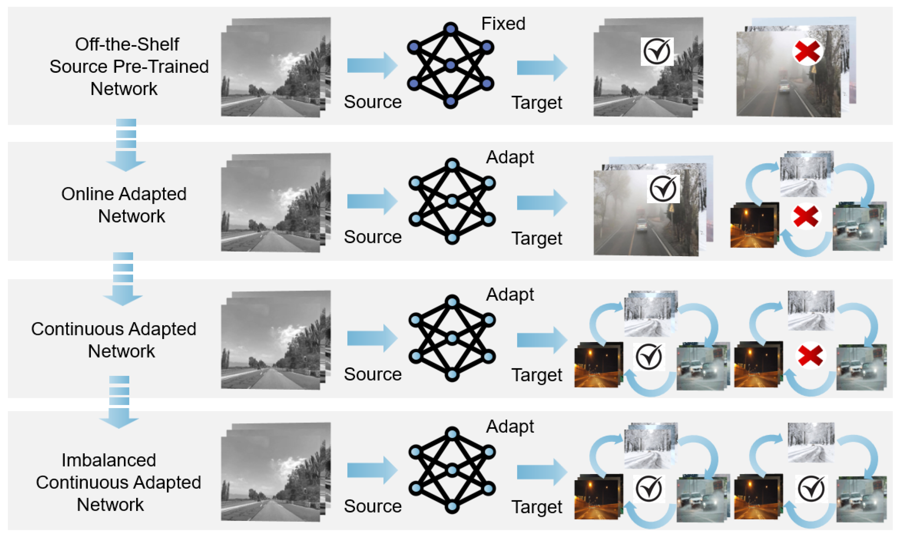
• To the best of our knowledge, we are the first to propose ICTTA, a novel test-time adaptation setting that explicitly addresses class imbalance in dynamically evolving test data streams, a challenge previously overlooked in CTTA research.
• We construct an imbalanced perturbation dataset that simulates real-world streaming data, enabling rigorous evaluation under dynamic conditions.
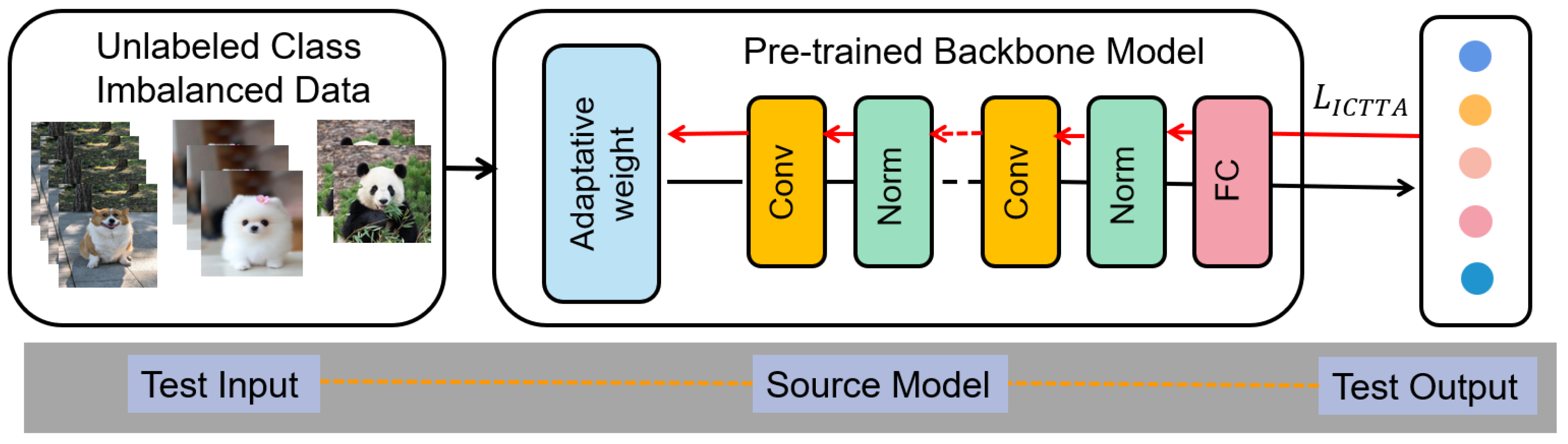
• We propose a class-aware adaptive loss function that dynamically adjusts loss weights based on real-time class distribution shifts, ensuring effective learning from minority classes while maintaining performance on majority classes. Furthermore, we provide a theoretical analysis demonstrating the effectiveness of our method in the ICTTA setting.
• Experiments on CIFAR and ImageNet demonstrate that our method significantly outperforms state-of-the-art TTA approaches, effectively mitigating performance degradation caused by class imbalance.

Figure 1 illustrates the differences between existing adaptation paradigms and our proposed ICTTA. Unlike conventional TTA and CTTA, which fail to address imbalanced learning in dynamic settings, our approach enables robust and adaptive test-time learning under continuously evolving conditions.

The remainder of this paper is organized as follows. Section 2 reviews related work. Section 3 formalizes the mathematical foundations of TTA, CTTA, and our proposed ICTTA, followed by a detailed discussion of our method’s core design. We also provide a theoretical analysis demonstrating its effectiveness in handling class imbalance. Section 4 presents extensive experiments on CIFAR and ImageNet, comparing our approach against state-of-the-art TTA methods using standard evaluation metrics. Finally, Section 5 concludes the paper with key insights and future directions.

To align this work with the scope of Symmetry, we emphasize how our proposed ICTTA framework engages with the principle of symmetry in the context of dynamic learning systems. In real-world test-time environments, class distributions are often imbalanced and evolve over time, which leads to a form of distributional asymmetry. Such asymmetry disrupts the balance that many existing adaptation methods implicitly rely on, resulting in biased model behavior that favors majority classes.

Our method, ICTTA, explicitly detects and mitigates this asymmetry by introducing a confidence-aware adaptive loss function. This mechanism dynamically adjusts the learning process to rebalance the influence of each class, thereby establishing predictive symmetry across evolving test-time distributions. The adaptive weighting strategy constitutes a symmetry restoration operation as it enforces equitable treatment across all classes regardless of their prevalence in the data stream.

More broadly, this work reflects a key principle in symmetry-aware systems: maintaining invariance or balanced treatment under transformations or distributional shifts. CTTA restores predictive symmetry through three fundamental principles: (1) Optimization symmetry: By balancing gradient magnitudes between classes (as shown in Theorem 1), ICTTA ensures fair parameter updates across decision boundaries. (2) Information-theoretic symmetry: The regularization encourages equal entropy contributions across classes, mitigating class-wise overconfidence. (3) Statistical symmetry: ICTTA maintains consistent performance under covariate shift, aligning class-conditional distributions to ensure robustness.

2. Related Work

2.1. Transfer Learning

Transfer learning [10,11] facilitates knowledge transfer from a well-established source domain to a related but distinct target domain. This process typically involves two stages: first, a model is pre-trained on a large-scale dataset to learn generalizable features; second, it is fine-tuned on a smaller, task-specific dataset to adapt to the target domain. By leveraging knowledge learned from abundant source data, transfer learning improves efficiency and mitigates overfitting, making it particularly valuable when labeled target data is scarce or expensive to obtain.

2.2. Domain Adaptation

Domain adaptation [12] is a specialized form of transfer learning that addresses distributional discrepancies between labeled source domains and unlabeled or sparsely labeled target domains [6]. Even when source and target domains share the same feature space, distribution shifts can hinder generalization. To mitigate this issue, domain adaptation methods learn domain-invariant representations via distribution alignment [10,13].

Notable approaches include feature alignment techniques such as deep adaptation networks (DANs) [10], which leverage multi-kernel maximum mean discrepancy (MK-MMD) to align distributions across multiple network layers. Additionally, adversarial training methods, such as domain-adversarial neural networks (DANNs) [12], employ adversarial objectives to encourage domain-invariant feature learning. These approaches enable models to effectively generalize across domains while mitigating sensitivity to domain-specific artifacts.

2.3. Domain Generalization

Domain generalization (DG) [14,15] extends transfer learning by training models to generalize to unseen target domains without direct exposure during training [16]. Unlike domain adaptation, which requires some target domain data for adaptation, DG aims to learn robust, domain-invariant features from multiple source domains [16], thereby preventing overfitting to any specific domain.

Style-based normalization techniques have emerged as powerful tools for domain generalization. For example, MixStyle [14] interpolates feature statistics from multiple domains during training to improve robustness. AdaBN [17] dynamically recalibrates batch normalization statistics during inference. These methods complement our work, though ICTTA operates without requiring style mixing or BN layer modifications.

Key DG strategies include meta-learning approaches such as MetaReg [18] and MASF [19], data augmentation techniques [20], and optimization-based methods guided by uncertainty principles. These methods extract fundamental, generalizable features, enabling robust model performance across diverse, unseen domains.

2.4. Test-Time Training

Test-time training (TTT) [21,22,23] is an emerging paradigm that enables models to dynamically adapt to new test samples during inference. Unlike conventional inference workflows, where models remain static after deployment, TTT optimizes parameters on incoming test data before making predictions by leveraging self-supervised auxiliary tasks.

This approach has proven effective in handling distributional shifts commonly encountered in real-world applications such as medical imaging and autonomous driving. By continuously refining representations at test time, TTT enhances model robustness while maintaining adaptability to evolving data distributions.

2.5. Test-Time Adaptation

Test-time adaptation (TTA) [24,25] has gained prominence as a practical approach for improving model generalization under distribution shifts by adapting parameters using unlabeled test data—without requiring access to the source dataset [26,27]. This paradigm is particularly valuable in privacy-sensitive and resource-constrained environments.

Many TTA techniques leverage batch normalization (BN) layers [28,29], which capture domain-specific statistics. For example, CD-TTA [30] employs a switchable BN mechanism using Bhattacharyya distance, while Core recalibrates BN statistics by interpolating between source and test-time distributions. Entropy minimization methods, such as TENT [24], refine BN affine parameters by minimizing prediction entropy, inspiring extensions like VMP [31], which formulates TENT within a probabilistic framework using variational Bayesian inference.

Beyond BN-based techniques, alternative TTA strategies include augmentation-based consistency learning (e.g., TTA-PR, which minimizes mean entropy across augmentations) and teacher–student frameworks (e.g., RMT, which enforces consistency between teacher and student predictions). Continual test-time adaptation (CTTA) [7] extends TTA by refining pseudo-labels across sequential test batches while incorporating weight-averaged updates across the entire network.

Despite these advancements, most TTA methods heavily rely on entropy minimization and global regularization, often neglecting the impact of class imbalance. Many prioritize majority-class optimization, leading to biased adaptation and suboptimal performance on rare but critical minority classes. This limitation underscores the need for adaptation techniques that explicitly address class imbalance in evolving test-time settings.

2.6. Class Imbalanced Learning

Class imbalance [32] poses a significant challenge in machine learning, particularly in domains such as fraud detection, medical diagnosis, and rare event prediction. Standard learning algorithms tend to favor majority classes, leading to subpar recognition of critical minority instances. This imbalance disrupts the symmetry of the learning process, causing models to perform unevenly across different classes.

Several strategies have been developed to mitigate class imbalance. Resampling techniques include oversampling the minority class and undersampling the majority class to balance distributions [33,34]. Cost-sensitive learning assigns higher penalties to misclassified minority samples, encouraging models to focus on these critical instances. Additionally, synthetic data generation methods such as SMOTE [35] create artificial minority samples to enhance representation learning.

More advanced approaches integrate ensemble learning and meta-learning techniques to improve model robustness in imbalanced settings. Recent innovations, including focal loss [32] and adaptive weighting strategies [31,36], further enhance the ability to learn from underrepresented classes while preventing majority class dominance.

In the context of test-time adaptation, class imbalance is an often-overlooked challenge. While traditional TTA techniques primarily focus on domain adaptation, they fail to account for real-world scenarios where the distribution of test-time data is highly imbalanced. Addressing this limitation requires novel adaptation strategies that dynamically adjust learning objectives based on evolving class distributions. Recent studies have proposed rebalancing replay buffers [37], online adaptation for imbalanced streams [38], and comprehensive surveys on challenges in this domain [39].

3. Method

3.1. Preliminaries

3.1.1. Test-Time Adaptation (TTA)

Given a pre-trained model $f_{\theta }:\mathcal{X}\to {\mathbb{R}}^C$ with parameters $\theta$, trained on a source domain dataset ${\mathcal{D}}_s$, our goal is to adapt the model to an unlabeled test dataset $x_i^t{i=1}^N\sim {\mathcal{D}}_t$ under distribution shift, where ${\mathcal{D}}_t\ne {\mathcal{D}}_s$. The network’s logits are denoted as z, and the softmax function is expressed as

$$p\left(y^t\right|x^t;\theta )={\displaystyle \frac{e^{z_i}}{{\sum }_{c=1}^C{e}^{z_c}}}$$

(1)

A widely used loss function in TTA is the standard entropy minimization objective [24], formulated as

$${\mathcal{L}}_{\mathrm{TENT}}={\displaystyle \frac{1}{N}}\sum _{i=1}^{N}H\left(p_i\right)$$

(2)

where $H\left(p_i\right)=-{\sum }_{c=1}^C{p}_{i,c}log{p}_{i,c}$ represents the entropy of the softmax probabilities $p_i=\mathrm{softmax}\left(f_{\theta }\left(x_i^t\right)\right)$.

3.1.2. Continual TTA (CTTA)

Following the established CTTA framework [7], we adopt two core components:

• A teacher–student framework with momentum updates:

  $${\theta }_{\mathrm{teacher}}\leftarrow m{\theta }_{\mathrm{teacher}}+(1-m)\theta$$

  (3)

  where m is the momentum coefficient ($0<m<1$).
• Augmentation anchoring:

  $${\mathcal{L}}_{\mathrm{CTTA}}={\displaystyle \frac{1}{N}}\sum _{i=1}^N{\parallel f_{\theta }\left(\mathcal{A}\left(x_i^t\right)\right)-f_{{\theta }_{\mathrm{teacher}}}\left(x_i^t\right)\parallel }^2$$

  (4)

CTTA is a well-established continual test-time adaptation method that employs a teacher–student network to mitigate prediction errors. Additionally, it selectively restores a small portion of the pre-trained weights to enhance adaptation under environmental changes.

3.2. Imbalanced Continual Test-Time Adaptation (ICTTA)

Existing TTA methods often overlook class imbalance, a common issue in real-world datasets. In this paper, we introduce ICTTA to address this limitation.

Given a pre-trained classifier $f_{\theta }:\mathcal{X}\to {\mathbb{R}}^C$ and an unlabeled test stream ${\left\{x_t\right\}}_{t=1}^T$, ICTTA operates without prior knowledge of the minority and majority classes. The only available information is the unlabeled test data. Figure 2 illustrates the core design of our proposed ICTTA method. The class-imbalanced test data stream is fed into a fixed, pre-trained backbone model to extract features. Based on the confidence margin computed for each sample, adaptive weights are assigned that modulate the contribution of each sample during model updates.

3.2.1. Supervision of Sample Difficulty

We leverage the confidence margin—the difference between the highest and second-highest confidence scores—as an indicator of sample difficulty. This margin is computed as

$$diff\left(f_{\theta }\left(x^t\right)\right)=conf{\left(f_{\theta }\left(x^t\right)\right)}_{1st}-conf{\left(f_{\theta }\left(x^t\right)\right)}_{2nd}$$

(5)

Here, $f_{\theta }\left(x^t\right)$ denotes the logit output at test time, and $conf\left(f_{\theta }\left(x^t\right)\right)$ represents the confidence scores after applying the softmax function. This measure quantifies the ambiguity of the model’s prediction—smaller values indicate higher uncertainty, necessitating stronger adaptation. To address this, we design an adaptive truncation function that assigns higher weights to ambiguous samples while reducing the influence of highly confident samples.

3.2.2. Confidence-Weighted Loss Design

To mitigate the impact of extreme outliers, we define a sample weight $w_i$ based on prediction confidence:

$$w_i=\left\{\begin{array}{cc}{(1-(p_i^{\left(1\right)}-p_i^{\left(2\right)}))}^{\gamma }\hfill & \mathrm{if}{p}_i^{\left(1\right)}>\tau \hfill \\ 0\hfill & \mathrm{otherwise}\hfill \end{array}\right.$$

(6)

where

• $p_i^{\left(1\right)}$ and $p_i^{\left(2\right)}$ are the highest and second-highest softmax probabilities for sample $x_i$.
• $\gamma$ is the focusing parameter ($\gamma \ge 0$) that controls the rate at which easy samples are down-weighted.
• $\tau$ is the confidence threshold ($0<\tau \le 1$) that determines the minimum confidence required for a sample to contribute to adaptation.

Our composite loss function integrates entropy minimization with class rebalancing:

$$\begin{array}{cc}\hfill {\mathcal{L}}_{\mathrm{ICTTA}}& =\underset{\mathrm{Entropy}\mathrm{Minimization}}{\underbrace{{\lambda }_1\mathbb{E}\left[H\left(p\right)\right]}}+\underset{\mathrm{Class}\mathrm{Rebalancing}}{\underbrace{{\lambda }_2\mathbb{E}[w·H\left(p\right)]}}\hfill \end{array}$$

(7)

$$\begin{array}{cc}\hfill & ={\displaystyle \frac{1}{N}}\sum _{i=1}^N\left({\lambda }_{1}H\left(p_i\right)+{\lambda }_2{w}_{i}H\left(p_i\right)\right)\hfill \end{array}$$

(8)

$$\begin{array}{cc}\hfill & ={\displaystyle \frac{1}{N}}\sum _{i=1}^C{\lambda }_1\left(-{\displaystyle \frac{e^{z_i}}{{\sum }_{c=1}^C{e}^{z_c}}}log\left({\displaystyle \frac{e^{z_i}}{{\sum }_{c=1}^C{e}^{z_c}}}\right)\right)+\hfill \end{array}$$

(9)

$$\begin{array}{cc}\hfill & {\lambda }_2{(1-(p_i^{\left(1\right)}-p_i^{\left(2\right)}))}^{\gamma }\left(-{\displaystyle \frac{e^{z_i}}{{\sum }_{c=1}^C{e}^{z_c}}}log\left({\displaystyle \frac{e^{z_i}}{{\sum }_{c=1}^C{e}^{z_c}}}\right)\right)\hfill \end{array}$$

(10)

where $H\left(p\right)=-{\sum }_{c=1}^C{p}_{c}log{p}_c$ is Shannon entropy, and w is the confidence-aware weight. The hyperparameters ${\lambda }_1$ and ${\lambda }_2$ balance adaptation stability and minority class preservation. Our objective is to prioritize difficult minority samples while reducing the weight of easy majority samples.

3.2.3. Theoretical Analysis

Theorem 1. 

For a C-class classification problem, where each class i has a predicted probability $p_i$ such that $0<p_i<1$ and ${\sum }_{i=1}^C{p}_i=1$, the proposed loss function ${\mathcal{L}}_{ICTTA}$ enhances adaptation for the minority class.

Proof. 

Let the predicted probability be defined as

$$p_i={\displaystyle \frac{e^{z_i}}{{\sum }_{c=1}^C{e}^{z_c}}},i=1,2,\dots ,C.$$

(11)

The proposed loss function consists of two terms:

$${\mathcal{L}}_{\mathrm{ICTTA}}={\lambda }_1\mathbb{E}\left[H\left(p\right)\right]+{\lambda }_2\mathbb{E}[w·H\left(p\right)],$$

(12)

where $H\left(p\right)=-{\sum }_{c=1}^C{p}_{c}log{p}_c$ is the Shannon entropy, and the weight term is defined as

$$w_i=\left\{\begin{array}{cc}{(1-(p_i^{\left(1\right)}-p_i^{\left(2\right)}))}^{\gamma },\hfill & \mathrm{if}{p}_i^{\left(1\right)}>\tau ,\hfill \\ 0,\hfill & \mathrm{otherwise}.\hfill \end{array}\right.$$

(13)

The coefficients ${\lambda }_1$ and ${\lambda }_2$ balance adaptation stability and minority class preservation.

Entropy Term Gradient. The entropy loss is

$$\mathbb{E}\left[H\left(p\right)\right]=-\sum _{i=1}^C{p}_{i}log{p}_i.$$

(14)

Its gradient with respect to $p_i$ is

$${\displaystyle \frac{\partial H}{\partial p_i}}=-log{p}_i-1.$$

(15)

Weighted Entropy Term Gradient. For the weighted entropy term,

$$\mathbb{E}[w·H\left(p\right)]=-\sum _{i=1}^C{w}_i{p}_{i}log{p}_i.$$

(16)

Its gradient with respect to $p_i$ is

$${\displaystyle \frac{\partial }{\partial p_i}}(w_i{p}_{i}log{p}_i)=w_i(-log{p}_i-1)+p_i{\displaystyle \frac{\partial w_i}{\partial p_i}}log{p}_i.$$

(17)

Confidence Weight Derivative.Since $w_i$ depends on $p_i$, we compute its derivative:

$${\displaystyle \frac{\partial w_i}{\partial p_i}}=-\gamma {(1-(p_i^{\left(1\right)}-p_i^{\left(2\right)}))}^{\gamma -1}·{\displaystyle \frac{\partial }{\partial p_i}}(p_i^{\left(1\right)}-p_i^{\left(2\right)}).$$

(18)

For minority classes, where $p_i^{\left(1\right)}$ is small, the confidence margin $(p_i^{\left(1\right)}-p_i^{\left(2\right)})$ is also small, leading to

$$w_i\approx 1,{\displaystyle \frac{\partial w_i}{\partial p_i}}\approx 0.$$

(19)

Gradient Analysis. For minority classes ($p_i$ is small), the loss gradient simplifies to

$${\displaystyle \frac{\partial }{\partial p_i}}{\mathcal{L}}_{ICTTA}\approx {\lambda }_1(-log{p}_i-1).$$

(20)

For majority classes, where $p_i$ is larger, $w_i$ is smaller, leading to relatively smaller gradients.

Gradient Comparison. To quantify the difference in updates, we define the ratio:

$$R={\displaystyle \frac{\left|\frac{\partial }{\partial p_{\min }}{\mathcal{L}}_{ICTTA}\right|}{\left|\frac{\partial }{\partial p_{\mathrm{maj}}}{\mathcal{L}}_{ICTTA}\right|}}={\displaystyle \frac{log{p}_{\mathrm{maj}}+1}{log{p}_{\min }+1}}.$$

(21)

Since $p_{\min }$ denotes the maximum predicted probability for a minority-class sample, it is typically lower than that for majority classes. As a result, $log{p}_{\min }+1$ is smaller, and thus R is greater than 1 in most practical scenarios. This implies that our loss function amplifies updates for minority classes compared to majority ones.

We conducted extensive experiments to evaluate the sensitivity of Theorem 1 to hyperparameters ${\lambda }_1$, ${\lambda }_2$, and $\gamma$. The results indicate that our method exhibits low sensitivity to these hyperparameters and maintains robust performance across a variety of configurations. This demonstrates that our approach is not overly dependent on their precise tuning.

ICTTA restores predictive symmetry through three fundamental principles: (1) Optimization symmetry: By balancing gradient magnitudes between classes (as shown in Theorem 1), ICTTA ensures fair parameter updates across decision boundaries. (2) Information-theoretic symmetry: The regularization encourages equal entropy contributions across classes, mitigating class-wise overconfidence. (3) Statistical symmetry: ICTTA maintains consistent performance under covariate shift, aligning class-conditional distributions to ensure robustness.

Conclusion. The proposed loss function ${\mathcal{L}}_{ICTTA}$ improves minority class adaptation by enhancing their gradient magnitudes. Unlike traditional entropy minimization, our approach effectively preserves information for underrepresented classes, ensuring better adaptation in class-imbalanced continual test-time learning.

Thus, we have demonstrated that ${\mathcal{L}}_{ICTTA}$ prioritizes minority class adaptation, yielding improved overall performance in imbalanced classification scenarios. □

3.3. Source Model and Auxiliary Information

Unlike previous approaches in test-time adaptation (TTA), which require modifications to the source model or additional auxiliary information during inference [8,25,26], the proposed ICTTA method operates without such dependencies.

For example, test-time training (TTT) requires retraining on the source data and introduces an auxiliary rotation prediction branch for target adaptation, thereby preventing the direct reuse of pre-trained models. Similarly, CTTA relies on additional test-time data augmentations, which can be considered as auxiliary information for enhancing adaptation.

In contrast, ICTTA leverages an off-the-shelf, source-pretrained model and adaptively updates its parameters to match the target distribution in an online manner, without requiring additional data or model modifications. The only added computations are straightforward confidence margin calculations and adaptive weighting applied on the current batch, which introduce minimal overhead. Empirically, across all evaluated benchmarks, we did not observe any noticeable increase in inference latency or memory consumption compared to standard model inference. This suggests that ICTTA can be practically integrated into off-the-shelf models with minimal impact on deployment efficiency.

Consequently, ICTTA is highly generalizable and can be seamlessly integrated with a wide range of pre-trained models, making it a versatile solution for real-world deployment scenarios.

4. Experiment

We conducted a comprehensive set of experiments to evaluate the effectiveness of the proposed ICTTA framework across two benchmark datasets for digital corruption: CIFAR10-C and ImageNet-C [40].

4.1. Benchmarks

4.1.1. Datasets

• CIFAR10-C: CIFAR10-C is an extension of the original CIFAR10 dataset, designed to assess model robustness against common image corruptions [20,40]. It has been subjected to 15 types of corruption, such as noise, blur, weather effects, each at 5 different severity levels.
• ImageNet-C: ImageNet-C is a large-scale dataset featuring 75 unique corruptions across 15 categories, including noise, blur, weather, and digital distortions. Each corruption type is tested at five severity levels. With 1000 classes, it is one of the largest and most widely used benchmarks for evaluating robustness to image corruptions.

4.1.2. Network Architectures

We evaluate the ICTTA framework’s generalization across three distinct network architectures:

• WideResNet-28-10: A popular architecture in the TTA literature, this model features 28 layers and a width of 10, providing a balanced capacity suitable for a wide range of tasks.
• WideResNet-40-2: This variant is characterized by a 40-layer depth and a width of 2, offering a different depth–width ratio to explore model performance from an alternative perspective.
• ResNet-50: The ResNet-50 architecture is a deep residual network with 50 layers, designed to address the vanishing gradient problem through residual connections. This network uses batch normalization and ReLU activations after each convolutional layer, which helps in improving gradient flow and accelerating training. It has become one of the most widely used architectures for various vision tasks due to its effectiveness in deep learning models.

4.1.3. Compared Methods

We compare ICTTA with several well-known baseline methods:

• Source: Direct application of the pre-trained model without adaptation. The baseline approach, where the pre-trained model is directly applied to the test data without any adaptation. This method serves as a control to assess the effectiveness of more sophisticated TTA strategies as it depends solely on the training data distribution, potentially leading to performance degradation under domain shifts or corrupted test data.
• BN Stats Adapt: Recalibration of batch normalization statistics using test data [24]. This method recalibrates the batch normalization (BN) statistics using the test data. It recomputes the running mean and variance during the test phase, allowing the model to adapt to the new data distribution. This approach is computationally efficient, requiring only a forward pass through the test data.
• TENT: Optimization of BN parameters via entropy minimization [24]. TENT builds upon BN Stats Adaptation by optimizing the scale and shift parameters of the BN layers through gradient-based backpropagation. The objective is to minimize the entropy of the model’s predictions, improving confidence and accuracy. This lightweight adaptation process strikes a balance between computational cost and performance enhancement.
• CTTA: Teacher–student framework with weight-averaged updates [7]. CTTA is a well-established method that utilizes a teacher–student framework to iteratively improve model performance during test-time adaptation. In this approach, a student network learns from the predictions of a teacher network, gradually minimizing prediction errors. To enhance adaptation under domain shifts, CTTA selectively restores a small subset of the pre-trained weights, allowing the model to better adjust to the changing environment while preserving essential knowledge from the source domain.

4.2. Experiments on CIFAR Dataset

The CIFAR10-C dataset [40] extends the original CIFAR10 benchmark to assess the robustness of image classification models under various corruptions. It introduces 15 distinct types of algorithmically generated corruptions, categorized into noise, blur, weather effects, and digital distortions. Each corruption type is evaluated at five severity levels, resulting in a total of 75 unique corruptions. This dataset provides a comprehensive evaluation of model performance under real-world image degradations and is widely adopted in the computer vision community to benchmark and improve model robustness.

4.2.1. Experimental Settings

For the experiments, we used the source-pretrained models from the RobustBench benchmark (https://robustbench.github.io/, accessed on 28 May 2025), ensuring that the results reported in this paper are reproducible. Specifically, for the CIFAR10-C corruption task, we followed the official public implementation of TENT on WideResNet-28-10 and WideResNet-40-2 architectures. Specifically, and the WideResNet-28-10 checkpoint was the default model from RobustBench [41], the WideResNet-40-2 model was sourced from [20]. For all experiments, we used the Adam optimizer with the following hyperparameters: learning rate of 0.001, exponential decay rate of 0.9, weight decay of 0, batch size of 200, and ${\lambda }_{\max }$ set to 5.

4.2.2. Experiment Results

The classification error rate is formally defined as

$$\mathrm{Error}\mathrm{Rate}={\displaystyle \frac{\mathrm{Number}\mathrm{of}\mathrm{Misclassified}\mathrm{Samples}}{\mathrm{Total}\mathrm{Test}\mathrm{Samples}}}\times 100\%$$

(22)

Classification error rate: For the CIFAR10-to-CIFAR10-C task, classification error rate serves as a crucial metric to evaluate how well the model adapts to corrupted data without requiring retraining on labeled samples.

WideResNet-28-10: ICTTA achieves a mean classification error rate of 16.5%, representing a substantial improvement over existing methods. Specifically, it outperforms Source (44.1%), BN Stats Adapt (21.8%), TENT (16.9%), and CTTA (18.0%). This notable reduction in error rate confirms ICTTA’s enhanced capability in overall error mitigation across different model architectures. These results are supported by the data presented in

Table 1. Classification error rate (%) for the CIFAR10-to-CIFAR10-C ICTTA task on WideResNet-28-10. Results were evaluated with the largest corruption severity level of 5. Lower is better.

Method	Gaussian	shot	impulse	defocus	glass	motion	zoom	snow	frost	fog	brightness	contrast	elastic_trans	pixelate	jpeg	Mean
Source	73.4	67.0	75.6	51.2	54.6	39.5	48.5	24.8	40.9	25.3	9.8	46.7	27.3	50.7	26.5	44.1
BN Stats Adapt	29.1	26.4	36.4	13.4	36.6	16.6	13.7	19.8	18.8	16.5	11.1	15.2	26.0	20.0	27.8	21.8
TENT	26.8	20.6	27.3	11.1	28.2	12.8	10.7	14.8	14.0	13.9	7.9	12.3	19.7	14.8	19.4	16.9
CTTA	26.3	23.0	28.1	12.5	29.5	14.4	12.5	17.6	16.4	14.4	9.8	12.1	19.9	14.9	19.2	18.0
ICTTA (Ours)	26.4	19.8	26.6	10.7	28.0	12.1	10.4	14.5	14.2	12.6	7.6	11.3	18.6	14.4	20.0	16.5

.

WideResNet-40-2: ICTTA achieves a mean error rate of 10.8%, outperforming Source (17.7%), BN Stats Adapt (16.0%), TENT (11.5%), and CTTA (14.8%). The significant drop in error rate demonstrates the effectiveness of our dynamic adaptive loss function in handling class imbalance and distribution shifts.The detailed error rate results can be found in

Table 2. Classification error rate (%) for the standard CIFAR10-to-CIFAR10-C ICTTA task on WideResNet-40-2. Results were evaluated with the largest corruption severity level of 5. Lower is better.

Method	Gaussian	shot	impulse	defocus	glass	motion	zoom	snow	frost	fog	brightness	contrast	elastic_trans	pixelate	jpeg	Mean
Source	28.4	21.6	24.4	9.5	20.0	11.6	10.2	13.5	14.8	18.2	8.4	20.4	14.1	37.1	13.0	17.7
BN Stats Adapt	18.8	17.3	22.4	10.7	24.4	12.2	12.5	14.9	15.3	16.3	10.0	13.8	18.0	15.6	18.4	16.0
TENT	15.8	11.1	14.8	7.8	16.6	9.2	8.1	10.3	9.5	12.1	7.3	9.5	14.8	10.7	14.8	11.5
CTTA	17.7	15.4	18.7	10.5	20.6	12.8	11.7	14.5	13.6	17.2	9.1	17.8	16.0	12.4	14.8	14.8
ICTTA (Ours)	15.9	10.6	14.7	7.4	16.0	8.7	7.7	9.6	8.7	10.8	6.8	8.1	13.3	9.6	14.0	10.8

.

The evaluation metrics are formally defined as follows:

$$\begin{array}{cc}\hfill \mathrm{Precision}& ={\displaystyle \frac{TP}{TP+FP}}\hfill \\ \hfill \mathrm{Recall}& ={\displaystyle \frac{TP}{TP+FN}}\hfill \\ \hfill \mathrm{F}1\text{-}\mathrm{score}& ={\displaystyle \frac{2\times \mathrm{Precision}\times \mathrm{Recall}}{\mathrm{Precision}+\mathrm{Recall}}}\hfill \end{array}$$

(23)

where $TP$, $FP$, and $FN$ represent true positives, false positives, and false negatives, respectively. All metrics are calculated using macro-averaging across classes.

Precision: Precision measures the proportion of true positive predictions among all positive predictions, serving as an indicator of the model’s ability to avoid false positives.

WideResNet-28-10: ICTTA achieves a mean precision of 80.2%, which is comparable to TENT (79.3%) and represents a substantial improvement over Source (66.5%) and BN Stats Adapt (72.8%). This indicates that ICTTA effectively reduces false positives during inference, crucial for applications like medical diagnosis where precision is paramount. These results are detailed in

Table 3. Precision for the standard CIFAR10-to-CIFAR10-C ICTTA task on WideResNet-28-10. Results were evaluated with the largest corruption severity level of 5. Higher is better.

Method	Gaussian	shot	impulse	defocus	glass	motion	zoom	snow	frost	fog	brightness	contrast	elastic_trans	pixelate	jpeg	Mean
Source	60.2	63.1	45.7	62.3	56.7	65.9	64.0	73.7	69.7	75.7	85.4	66.4	70.8	68.5	69.6	66.5
BN Stats Adapt	65.8	67.5	59.1	80.7	60.2	77.4	80.6	74.8	75.2	77.7	83.1	79.0	69.2	74.2	66.8	72.8
TENT	68.0	73.5	66.6	84.8	66.1	83.0	86.3	81.6	82.8	83.5	89.7	85.5	77.6	82.7	78.3	79.3
CTTA	68.7	70.9	67.0	81.8	65.4	79.5	81.9	76.2	77.3	79.8	84.3	82.1	73.6	78.9	74.4	76.1
ICTTA (Ours)	68.2	74.4	67.7	86.2	67.1	85.4	87.5	84.2	84.5	85.5	90.6	85.4	77.2	82.9	76.9	80.2

.

WideResNet-40-2: ICTTA attains a mean precision of 86.8%, outperforming Source (80.5%), BN Stats Adapt (78.3%), TENT (86.0%), and CTTA (79.9%). The high precision values suggest robust performance in identifying critical minority classes across various corruption types. Recall Analysis Recall measures the model’s ability to identify all relevant instances, which is essential for ensuring that critical cases are not missed. The precision results are further illustrated in

Table 4. Precision for the standard CIFAR10-to-CIFAR10-C ICTTA task on WideResNet-40-2. Results were evaluated with the largest corruption severity level of 5. Higher is better.

Method	Gaussian	shot	impulse	defocus	glass	motion	zoom	snow	frost	fog	brightness	contrast	elastic_trans	pixelate	jpeg	Mean
Source	74.4	78.1	72.5	87.6	76.8	83.8	85.7	82.8	81.4	81.5	86.6	78.2	82.0	73.4	83.1	80.5
BN Stats Adapt	75.6	76.9	71.8	83.7	70.5	82.0	82.1	79.3	78.7	78.0	84.4	80.1	76.4	78.8	75.9	78.3
TENT	78.6	84.9	81.3	89.9	79.8	88.4	89.6	86.9	88.3	85.9	91.2	89.3	83.1	87.9	84.1	86.0
CTTA	77.3	79.1	76.0	84.1	74.6	81.8	83.0	80.4	80.9	77.5	85.4	77.3	78.8	82.4	79.7	79.9
ICTTA (Ours)	78.4	84.9	80.9	90.5	80.3	89.6	91.1	88.4	90.8	87.2	91.6	90.2	84.5	89.4	83.8	86.8

.

Recall: Recall measures the model’s ability to identify all relevant instances, ensuring that critical cases are not overlooked. WideResNet-28-10: ICTTA achieves a mean Recall of 79.9%, slightly below TENT (80.1%) but surpassing Source (56.4%) and BN Stats Adapt (79.2%). This means ICTTA successfully identifies more true positives while maintaining a balance between precision and Recall. The recall results are presented in

Table 5. Recall for the standard CIFAR10-to-CIFAR10-C ICTTA task on WideResNet-28-10. Results were evaluated with the largest corruption severity level of 5. Higher is better.

Method	Gaussian	shot	impulse	defocus	glass	motion	zoom	snow	frost	fog	brightness	contrast	elastic_trans	pixelate	jpeg	Mean
Source	27.0	34.3	27.1	53.0	46.8	65.7	58.5	74.5	57.4	74.4	90.3	53.8	72.5	41.0	70.0	56.4
BN Stats Adapt	71.6	73.8	64.4	87.2	65.1	84.6	87.8	81.7	81.9	85.0	90.3	86.0	75.4	80.7	72.4	79.2
TENT	73.4	77.6	70.5	87.9	67.9	85.3	87.5	81.5	81.7	82.9	90.0	85.0	75.1	80.1	74.5	80.1
CTTA	74.8	77.1	73.0	87.6	70.3	85.7	88.1	82.6	83.0	86.2	90.5	87.9	78.9	84.1	79.6	82.0
ICTTA (Ours)	73.9	78.2	70.7	87.8	66.7	84.8	86.1	80.7	80.5	82.9	90.0	86.0	75.8	80.0	74.4	79.9

.

WideResNet-40-2: ICTTA achieves a mean Recall of 86.1%, outperforming Source (81.7%), BN Stats Adapt (84.9%), TENT (85.8%), and CTTA (86.1%). The high Recall values indicate that ICTTA effectively captures critical minority instances, crucial for applications where missing a positive case could have severe consequences.

Table 6. Recall for the standard CIFAR10-to-CIFAR10-C ICTTA task on WideResNet-40-2. Results were evaluated with the largest corruption severity level of 5. Higher is better.

Method	Gaussian	shot	impulse	defocus	glass	motion	zoom	snow	frost	fog	brightness	contrast	elastic_trans	pixelate	jpeg	Mean
Source	71.4	77.0	75.9	90.1	78.8	89.4	90.6	85.9	83.8	82.2	91.7	79.3	85.0	58.4	85.4	81.7
BN Stats Adapt	82.4	83.9	78.5	90.1	76.7	88.9	88.8	86.2	85.4	84.9	91.1	86.5	82.8	85.3	82.7	84.9
TENT	84.3	88.0	82.9	91.3	80.1	88.9	89.9	86.4	86.6	84.5	90.1	87.8	80.3	84.8	80.8	85.8
CTTA	84.0	85.8	82.3	90.4	80.6	88.1	89.4	86.7	87.1	84.0	91.7	82.5	84.7	88.6	85.9	86.1
ICTTA (Ours)	84.3	88.5	82.5	91.2	79.5	88.5	89.7	86.0	86.8	84.7	90.7	89.4	81.4	86.3	82.2	86.1

provides the detailed recall results.

F1-score: The F1-score, which balances precision and Recall, provides a comprehensive measure of the model’s performance in handling both false positives and false negatives.

WideResNet-28-10: ICTTA achieves a mean F1-score of 79.4%, outperforming Source (52.9%), BN Stats Adapt (73.8%), TENT (78.8%), and CTTA (77.6%).The F1-score results are shown in

Table 7. F1 for the standard CIFAR10-to-CIFAR10-C ICTTA task on WideResNet-28-10. Results were evaluated with the largest corruption severity level of 5. Higher is better.

Method	Gaussian	shot	impulse	defocus	glass	motion	zoom	snow	frost	fog	brightness	contrast	elastic_trans	pixelate	jpeg	Mean
Source	23.1	30.8	20.5	50.0	40.4	60.2	52.3	71.9	56.8	72.9	86.4	52.1	68.9	39.8	68.1	52.9
BN Stats Adapt	66.3	68.7	59.0	82.6	59.4	79.0	82.5	75.8	76.5	79.4	84.9	80.3	69.7	75.4	67.4	73.8
TENT	68.7	74.5	67.2	85.8	65.4	83.4	86.2	80.9	81.8	82.6	89.5	84.6	75.6	80.8	75.6	78.8
CTTA	69.3	72.3	67.7	83.9	65.4	81.4	83.8	77.8	79.0	81.7	86.3	84.0	75.1	80.6	75.9	77.6
ICTTA (Ours)	69.0	75.3	68.0	86.7	65.4	84.7	86.4	81.8	81.9	83.8	90.1	85.4	76.0	81.0	75.1	79.4

.

WideResNet-40-2: ICTTA achieves a mean F1-score of 86.8%, outperforming Source (79.2%), BN Stats Adapt (79.9%), TENT (85.4%), and CTTA (81.3%). These high F1-scores demonstrate ICTTA’s effectiveness in managing the precision–Recall trade-off under complex dataset conditions.

Table 8. F1 for the standard CIFAR10-to-CIFAR10-C ICTTA task on WideResNet-40-2. Results were evaluated with the largest corruption severity level of 5. Higher is better.

Method	Gaussian	shot	impulse	defocus	glass	motion	zoom	snow	frost	fog	brightness	contrast	elastic_trans	pixelate	jpeg	Mean
Source	70.3	76.2	72.0	88.5	75.4	85.4	87.3	83.2	81.5	80.3	88.2	76.4	82.4	58.0	83.7	79.2
BN Stats Adapt	76.9	78.6	72.9	85.8	71.1	84.0	84.1	81.1	80.4	79.7	86.4	81.6	77.6	80.3	77.5	79.9
TENT	80.2	86.1	81.6	90.4	79.0	88.4	89.6	86.5	87.3	84.9	90.4	88.2	81.2	86.0	82.0	85.4
CTTA	78.6	80.7	76.9	86.2	75.2	83.3	84.8	81.9	82.5	78.7	87.4	77.5	80.1	83.9	81.2	81.3
ICTTA (Ours)	78.4	84.9	80.9	90.5	80.3	89.6	91.1	88.4	90.8	87.2	91.6	90.2	84.5	89.4	83.8	86.8

offers a detailed overview of the F1-score results.

In the CIFAR10-to-CIFAR10-C task, ICTTA demonstrates strong adaptability in handling both data distribution shifts and class imbalance. For WideResNet-28-10, ICTTA reduces the classification error rate from 44.1% (Source) to 16.5% while outperforming competing methods in key metrics such as precision, Recall, and F1-score—particularly excelling in minimizing false positives. On the deeper WideResNet-40-2 model, ICTTA further decreases the error rate to 10.8% and excels in all evaluation metrics, with an outstanding F1-score of 86.8%. These results highlight ICTTA’s balanced performance across various architectures and its effectiveness in high-precision and high-Recall scenarios. Overall, ICTTA improves model adaptation and robustness, making it highly effective across diverse corruption types and domain shifts.

As illustrated in Figure 3 and Figure 4, the proposed ICTTA method demonstrates superior performance across both CIFAR10-to-CIFAR10-C datasets with WideResNet-28-10 and WideResNet-40-2 architectures. In both cases, ICTTA achieves the lowest classification error rate while maintaining high precision, recall, and F1-score. This highlights ICTTA’s effectiveness in addressing class imbalance and improving model adaptation in dynamically evolving test data streams, regardless of the model architecture.

4.3. Experiments on the ImageNet Dataset

To further validate the robustness of the proposed ICTTA framework, we evaluated its performance in the challenging ImageNet-to-ImageNet-C scenario. With 1000 classes, ImageNet-C presents a more complex environment compared to CIFAR-10 dataset, providing a more demanding testbed for assessing model resilience under various image corruptions.

4.3.1. Experimental Settings

For the ImageNet-C dataset, we employed a standard pre-trained ResNet-50 model, provided by RobustBench [41]. We utilized the SGD optimizer with the following hyperparameters: a learning rate of 0.00025, an exponential decay rate of 0.9, ${\lambda }_{max}$ set to 5, weight decay set to 0, and a batch size of 64. These settings were kept consistent to ensure fair comparisons across different methods.

4.3.2. Experiment Results

Classification error rate:As shown in

Table 9. Classification error rate (%) for the standard ImageNet-to-ImageNet-C ICTTA task. Results were evaluated on ResNet-50 with the largest corruption severity level of 5. Lower is better.

Method	Gaussian	shot	impulse	defocus	glass	motion	zoom	snow	frost	fog	brightness	contrast	elastic_trans	pixelate	jpeg	Mean
Source	93.7	93.7	92.9	86.0	91.4	87.5	76.7	84.8	80.2	78.1	45.9	95.3	86.9	74.5	66.1	82.2
BN Stats Adapt	87.9	88.6	85.9	87.9	89.0	78.9	66.5	69.4	71.0	55.8	38.5	89.2	63.0	58.1	69.6	73.3
TENT	86.5	83.8	79.4	83.6	81.9	71.7	60.9	66.9	65.6	55.1	40.7	79.1	56.9	54.2	60.8	68.5
CTTA	88.3	87.1	82.9	84.6	84.8	74.9	67.4	67.8	66.9	58.1	47.5	74.6	57.3	52.8	57.1	70.2
ICTTA (Ours)	86.4	83.3	78.7	83.1	80.8	71.3	60.5	66.8	65.9	55.0	41.3	78.0	57.4	53.3	60.0	68.1

, ICTTA significantly reduces classification error rates. Compared to the Source method, ICTTA achieves a substantial decrease in the mean error rate, dropping from 82.2% to 68.1%. This indicates ICTTA’s effectiveness in adapting to test data distribution shifts and mitigating the impact of class imbalance. Notably, ICTTA achieves significant error rate reductions in Gaussian, shot, and impulse noise categories, demonstrating its advantage in handling these common and challenging data corruptions.

Precision: The precision results in

Table 10. Precision for the standard ImageNet-to-ImageNet-C ICTTA task. Results were evaluated on ResNet-50 with the largest corruption severity level of 5. Higher is better.

Method	Gaussian	shot	impulse	defocus	glass	motion	zoom	snow	frost	fog	brightness	contrast	elastic_trans	pixelate	jpeg	Mean
Source	5.4	7.0	7.4	12.3	7.8	12.3	23.2	16.8	22.6	26.6	53.6	4.5	15.4	27.2	35.0	18.5
BN Stats Adapt	11.5	11.3	12.7	11.2	10.4	20.7	34.0	31.1	29.4	43.5	61.3	10.5	35.2	41.3	29.6	26.2
TENT	13.1	16.0	19.3	15.8	17.3	28.0	38.0	33.4	33.9	44.7	59.8	20.5	43.1	45.2	37.5	31.0
CTTA	11.8	14.0	15.7	14.2	14.7	24.2	33.7	33.0	31.6	42.4	53.4	24.6	42.3	47.6	41.0	29.6
ICTTA (Ours)	13.1	16.4	19.8	16.2	18.2	27.8	39.0	33.5	33.2	44.4	59.3	20.3	42.3	46.8	38.0	31.2

indicate that ICTTA achieves higher precision values in most corruption types. For instance, in the Gaussian corruption type, ICTTA’s precision is 13.1%, compared to 5.4% for Source and 11.5% for BN Stats Adapt. This means ICTTA can more accurately distinguish between positive and negative samples, reducing false positives, which is crucial in applications with low tolerance for false alarms such as medical diagnosis and security surveillance.

Recall:

Table 11. Recall for the standard ImageNet-to-ImageNet-C ICTTA task. Results were evaluated on ResNet-50 with the largest corruption severity level of 5. Higher is better.

Method	Gaussian	shot	impulse	defocus	glass	motion	zoom	snow	frost	fog	brightness	contrast	elastic_trans	pixelate	jpeg	Mean
Source	6.1	6.0	7.7	15.2	10.0	13.0	22.9	15.4	20.8	23.2	54.8	4.3	14.3	26.4	35.4	18.4
BN Stats Adapt	12.3	11.7	13.6	12.3	11.9	22.4	35.2	32.5	30.2	45.5	63.6	10.1	40.2	43.1	31.7	27.8
TENT	13.9	16.6	20.2	16.6	20.0	29.4	39.6	34.9	35.7	47.0	61.4	20.1	45.9	46.7	40.3	32.6
CTTA	12.3	13.4	17.1	15.2	16.5	26.4	34.1	34.4	33.9	43.5	54.5	25.1	44.8	49.1	43.9	30.9
ICTTA (Ours)	14.1	17.2	21.1	17.0	20.8	29.4	40.1	34.9	35.0	46.6	60.6	21.0	45.3	47.8	40.6	32.8

’s Recall data shows that ICTTA also performs well in identifying all relevant instances. In several corruption types like defocus, glass, and motion, ICTTA outperforms other methods in Recall. For defocus, ICTTA’s Recall rate is 17.0%, compared to 15.2% for Source and 12.3% for BN Stats Adapt. This suggests ICTTA is more effective in capturing critical minority instances, ensuring important detection targets are not missed in practical applications.

F1-score: Finally, the F1-scores, shown in

Table 12. F1 for the standard ImageNet-to-ImageNet-C ICTTA task. Results were evaluated on ResNet-50 with the largest corruption severity level of 5. Higher is better.

Method	Gaussian	shot	impulse	defocus	glass	motion	zoom	snow	frost	fog	brightness	contrast	elastic_trans	pixelate	jpeg	Mean
Source	4.7	5.2	6.0	11.4	6.9	10.6	19.6	14.1	18.8	21.8	50.6	3.5	12.5	23.2	31.4	16.0
BN Stats Adapt	10.5	9.9	11.6	10.3	9.6	19.4	31.6	28.8	26.7	41.3	59.5	8.7	34.4	39.1	27.7	24.6
TENT	11.9	14.3	17.7	14.4	16.1	25.9	35.9	31.2	31.8	42.6	57.8	18.2	40.8	43.0	35.9	29.2
CTTA	10.3	11.9	14.5	13.1	13.6	22.9	30.5	30.2	29.5	39.6	50.6	22.4	39.6	44.4	39.1	27.5
ICTTA (Ours)	11.9	14.7	18.4	14.7	16.9	26.0	36.6	31.1	31.2	42.3	57.0	18.5	40.1	44.0	36.5	29.3

, provide a balanced evaluation of precision and recall. ICTTA achieves an impressive average F1-score of 29.3%, higher than Source (16.0%), BN Stats Adapt (24.6%), and TENT (29.2%). This demonstrates ICTTA’s ability to effectively balance false positives and false negatives, making it well suited for applications that require a balanced approach to both precision and recall.

The performance results for the ImageNet-to-ImageNet-C dataset are visually summarized in Figure 5. ICTTA shows remarkable improvements in classification error reduction and achieves a good balance between precision and recall, as indicated by the highest F1-score. These results confirm the robustness and generalizability of ICTTA across different datasets and model architectures.

5. Conclusions

In this paper, we introduce ICTTA, a novel framework for imbalanced continuous test-time adaptation. To assess the effectiveness of our approach, we construct an imbalanced perturbation dataset based on CIFAR and ImageNet, revealing the shortcomings of existing CTTA methods in handling such challenging scenarios. Our analysis demonstrates that current methods fail to effectively address imbalanced test-time distributions. To bridge this gap, we propose a dynamic adaptive imbalanced loss function that assigns adaptive weights to each sample, thereby improving the model’s ability to handle distribution shifts and class imbalance. Additionally, we provide a theoretical analysis showing that our proposed loss function enhances adaptation for minority classes, proving its efficacy in ICTTA.

Extensive experiments conducted on CIFAR and ImageNet datasets validate the superior performance of ICTTA. Our method significantly outperforms existing baselines, including Source, BN Stats Adapt, TENT, and CTTA, achieving substantial improvements in key metrics. Specifically, ICTTA reduces classification error rates and simultaneously boosts precision, recall, and F1-scores. These results underscore the potential of ICTTA to effectively adapt to imbalanced and corrupted test-time data, establishing it as a powerful solution for real-world applications involving domain shifts and imbalanced data distributions.

While ICTTA demonstrates strong performance in current benchmarks, its robustness under highly dynamic or adversarial conditions warrants further investigation. Future work could explore enhanced mechanisms for real-time adaptation and outlier detection.

References

1. He, K.; Zhang, X.; Ren, S.; Sun, J. Deep residual learning for image recognition. In Proceedings of the IEEE Conference on Computer Vision and Pattern Recognition, Las Vegas, NV, USA, 27–30 June 2016; pp. 770–778. [Google Scholar]
2. Long, J.; Shelhamer, E.; Darrell, T. Fully convolutional networks for semantic segmentation. In Proceedings of the IEEE Conference on Computer Vision and Pattern Recognition, Boston, MA, USA, 7–12 June 2015; pp. 3431–3440. [Google Scholar]
3. Yu, H.; Luo, Y.; Shu, M.; Huo, Y.; Yang, Z.; Shi, Y.; Guo, Z.; Li, H.; Hu, X.; Yuan, J.; et al. DAIR-V2X: A Large-Scale Dataset for Vehicle-Infrastructure Cooperative 3D Object Detection. In Proceedings of the IEEE/CVF Conference on Computer Vision and Pattern Recognition, New Orleans, LA, USA, 18–24 June 2022; pp. 21361–21370. [Google Scholar]
4. Zhang, M.; Tian, X. Transformer architecture based on mutual attention for image-anomaly detection. Virtual Real. Intell. Hardw. 2023, 5, 57–67. [Google Scholar] [CrossRef]
5. Weng, W.; Pratama, M.; Za’in, C.; de Carvalho, M.; Appan, R.; Ashfahani, A.; Yee, E.Y.K. Autonomous Cross Domain Adaptation Under Extreme Label Scarcity. IEEE Trans. Neural Netw. Learn. Syst. 2022, 33, 7894–7907. [Google Scholar] [CrossRef]
6. Li, K.; Lu, J.; Zuo, H.; Zhang, G. Source-free multi-domain adaptation with fuzzy rule-based deep neural networks. IEEE Trans. Fuzzy Syst. 2023, 31, 4180–4194. [Google Scholar] [CrossRef]
7. Wang, Q.; Fink, O.; Van Gool, L.; Dai, D. Continual Test-Time Domain Adaptation. In Proceedings of the IEEE/CVF Conference on Computer Vision and Pattern Recognition, New Orleans, LA, USA, 18–24 June 2022; pp. 1234–1243. [Google Scholar]
8. Zhou, A.; Levine, S. Training on test data with bayesian adaptation for covariate shift. arXiv 2021, arXiv:2109.12746. [Google Scholar]
9. Zhu, J.; Li, W.; Wang, X. Clustering Environment Aware Learning for Active Domain Adaptation. IEEE Trans. Syst. Man Cybern. Syst. 2024, 54, 610–623. [Google Scholar] [CrossRef]
10. Long, M.; Cao, Y.; Wang, J.; Jordan, M.I. Learning transferable features with deep adaptation networks. In Proceedings of the International Conference on Machine Learning, PMLR, Lille, France, 6–11 July 2015; pp. 97–105. [Google Scholar]
11. Pan, S.J.; Yang, Q. A survey on transfer learning. IEEE Trans. Knowl. Data Eng. 2009, 22, 1345–1359. [Google Scholar] [CrossRef]
12. Ganin, Y.; Lempitsky, V. Unsupervised domain adaptation by backpropagation. In Proceedings of the International Conference on Machine Learning, PMLR, Lille, France, 6–11 July 2015; pp. 1180–1189. [Google Scholar]
13. Ganin, Y.; Ustinova, E.; Ajakan, H.; Germain, P.; Larochelle, H.; Laviolette, F.; March, M.; Lempitsky, V. Domain-adversarial training of neural networks. J. Mach. Learn. Res. 2016, 17, 1–35. [Google Scholar]
14. Zhou, K.; Yang, Y.; Qiao, Y.; Hospedales, T. Domain Generalization with MixStyle. In Proceedings of the International Conference on Learning Representations, Online, 3–7 May 2021. [Google Scholar]
15. Zhou, K.; Liu, Z.; Qiao, Y.; Xiang, T.; Loy, C.C. Domain generalization: A survey. IEEE Trans. Pattern Anal. Mach. Intell. 2022, 44, 4396–4415. [Google Scholar] [CrossRef]
16. Muandet, K.; Balduzzi, D.; Schölkopf, B. Domain generalization via invariant feature representation. In Proceedings of the International Conference on Machine Learning, Atlanta, GA, USA, 16–21 June 2013; pp. 10–18. [Google Scholar]
17. Liu, Y.; Kothari, P.; van Delft, B.; Bellot-Gurlet, B.; Mordan, T.; Alahi, A. Adaptive Batch Normalization for Practical Domain Adaptation. Pattern Recognit. Lett. 2021, 148, 56–63. [Google Scholar] [CrossRef]
18. Balaji, Y.; Sankaranarayanan, S.; Chellappa, R. Metareg: Towards domain generalization using meta-regularization. In Proceedings of the Advances in Neural Information Processing Systems, Montréal, QC, Canada, 3–8 December 2018; Volume 31, pp. 998–1008. [Google Scholar]
19. Dou, Q.; Coelho de Castro, D.; Kamnitsas, K.; Glocker, B. Domain generalization via model-agnostic learning of semantic features. In Proceedings of the Advances in Neural Information Processing Systems, Vancouver, BC, Canada, 8–14 December 2019; Volume 32, pp. 1–12. [Google Scholar]
20. Hendrycks, D.; Mu, N.; Cubuk, E.D.; Zoph, B.; Gilmer, J.; Lakshminarayanan, B. Augmix: A simple data processing method to improve robustness and uncertainty. arXiv 2019, arXiv:1912.02781. [Google Scholar]
21. Sun, Y.; Wang, X.; Liu, Z.; Miller, J.; Efros, A.; Hardt, M. Test-time training with self-supervision for generalization under distribution shifts. In Proceedings of the International Conference on Machine Learning, PMLR, Virtual, 13–18 July 2020; pp. 9229–9248. [Google Scholar]
22. Liu, Y.; Kothari, P.; van Delft, B.; Bellot-Gurlet, B.; Mordan, T.; Alahi, A. Ttt++: When does self-supervised test-time training fail or thrive? In Proceedings of the Advances in Neural Information Processing Systems, Online, 6–14 December 2021; Volume 34, pp. 21808–21820. [Google Scholar]
23. Gandelsman, Y.; Sun, Y.; Chen, X.; Efros, A. Test-time training with masked autoencoders. In Proceedings of the Advances in Neural Information Processing Systems, New Orleans, LA, USA, 28 November–9 December 2022; Volume 35, pp. 29374–29385. [Google Scholar]
24. Wang, D.; Shelhamer, E.; Liu, S.; Olshausen, B.; Darrell, T. Tent: Fully test-time adaptation by entropy minimization. In Proceedings of the International Conference on Learning Representations, Online, 3–7 May 2021. [Google Scholar]
25. Liang, J.; Hu, D.; Feng, J. Do we really need to access the source data? Source hypothesis transfer for unsupervised domain adaptation. In Proceedings of the International Conference on Machine Learning, PMLR, Virtual, 13–18 July 2020; pp. 6028–6039. [Google Scholar]
26. Mummadi, C.K.; Hutmacher, R.; Rambach, K.; Levinkov, E.; Brox, T.; Metzen, J.H. Test-time adaptation to distribution shift by confidence maximization and input transformation. arXiv 2021, arXiv:2106.14999. [Google Scholar]
27. You, F.; Li, J.; Zhao, Z. Test-time batch statistics calibration for covariate shift. arXiv 2021, arXiv:2110.04065. [Google Scholar]
28. Ioffe, S.; Szegedy, C. Batch normalization: Accelerating deep network training by reducing internal covariate shift. In Proceedings of the International Conference on Machine Learning, PMLR, Lille, France, 6–11 July 2015; pp. 448–456. [Google Scholar]
29. Ulyanov, D.; Vedaldi, A.; Lempitsky, V. Instance normalization: The missing ingredient for fast stylization. arXiv 2016, arXiv:1607.08022. [Google Scholar]
30. Song, J.; Park, K.; Shin, I.; Woo, S.; Kweon, I.S. CD-TTA: Compound Domain Test-time Adaptation for Semantic Segmentation. arXiv 2022, arXiv:2212.08356. [Google Scholar]
31. Jing, M.; Zhen, X.; Li, J.; Snoek, C. Variational model perturbation for source-free domain adaptation. In Proceedings of the Advances in Neural Information Processing Systems, New Orleans, LA, USA, 28 November–9 December 2022; Volume 35, pp. 17173–17187. [Google Scholar]
32. Lin, T.Y.; Goyal, P.; Girshick, R.; He, K.; Dollár, P. Focal loss for dense object detection. In Proceedings of the IEEE International Conference on Computer Vision, Venice, Italy, 22–29 October 2017; pp. 2980–2988. [Google Scholar]
33. He, H.; Garcia, E.A. Learning from imbalanced data. IEEE Trans. Knowl. Data Eng. 2009, 21, 1263–1284. [Google Scholar]
34. Chawla, N.V.; Bowyer, K.W.; Hall, L.O.; Kegelmeyer, W.P. SMOTE: Synthetic minority over-sampling technique. J. Artif. Intell. Res. 2002, 16, 321–357. [Google Scholar] [CrossRef]
35. Sun, P.; Wang, Z.; Jia, L.; Xu, Z. SMOTE-kTLNN: A hybrid re-sampling method based on SMOTE and a two-layer nearest neighbor classifier. Expert Syst. Appl. 2024, 238, 121848. [Google Scholar] [CrossRef]
36. Hu, X.; Uzunbas, G.; Chen, S.; Wang, R.; Shah, A.; Nevatia, R.; Lim, S.N. Mixnorm: Test-time adaptation through online normalization estimation. arXiv 2021, arXiv:2110.11478. [Google Scholar]
37. Lee, S.; Kim, J.; Hong, J. Rebalancing Replay Buffer for Class-Imbalanced Continual Learning. Neurocomputing 2024, 580, 1–10. [Google Scholar]
38. Wang, Y.; Zhang, L.; Chen, H. Online Test-Time Adaptation with Imbalanced Data Streams. IEEE Trans. Pattern Anal. Mach. Intell. 2023, 45, 10234–10247. [Google Scholar]
39. Zhang, R.; Wang, M.; Zhao, X. A Survey on Class-Imbalanced Continual Learning: Challenges, Methods, and Future Directions. ACM Comput. Surv. 2024, 56, 1–35. [Google Scholar]
40. Hendrycks, D.; Dietterich, T.G. Benchmarking neural network robustness to common corruptions and perturbations. arXiv 2019, arXiv:1903.12261. [Google Scholar]
41. Croce, F.; Andriushchenko, M.; Sehwag, V.; Debenedetti, E.; Flammarion, N.; Chiang, M.; Mittal, P.; Hein, M. RobustBench: A standardized adversarial robustness benchmark. In Proceedings of the Thirty-Fifth Conference on Neural Information Processing Systems Datasets and Benchmarks Track, Online, 6–14 December 2021. [Google Scholar]
Figure 1. Overview of the imbalanced continuous test-time adaptation (ICTTA) framework. The target data arrives as a sequential stream from a dynamically changing environment, where class distributions may shift over time. Initially, the model is a source-pretrained network. During online adaptation, the model continuously updates itself using the incoming imbalanced target data. This process involves (1) receiving test samples sequentially, (2) estimating confidence margins per sample to assess uncertainty, (3) assigning adaptive weights that balance the influence of imbalanced classes, and (4) optimizing the model parameters with the proposed adaptive loss function. Unlike existing methods that suffer from severe performance degradation under class imbalance, ICTTA maintains robust performance over long-term continuous adaptation.
Symmetry 17 01050 g001
Figure 2. Illustration of our proposed ICTTA method. The class-imbalanced test data stream is fed into a fixed, pre-trained backbone model to extract features. Based on the confidence margin computed for each sample, adaptive weights are assigned that modulate the contribution of each sample during model updates. These weighted samples are then used to optimize the model through our specifically designed loss function, which addresses the challenges posed by imbalanced continual test-time adaptation.
Symmetry 17 01050 g002
Figure 3. Performance comparison of different methods on CIFAR10-to-CIFAR10-C (WideResNet-28-10). The figure shows the mean values of classification error, precision, recall, and F1-score for each method.
Symmetry 17 01050 g003
Figure 4. Performance comparison of different methods on CIFAR10-to-CIFAR10-C (WideResNet-40-2). The figure displays the mean values of classification error, precision, recall, and F1-score for each method.
Symmetry 17 01050 g004
Figure 5. Performance comparison of different methods on ImageNet-to-ImageNet-C. The figure presents the mean values of classification error, precision, recall, and F1-score for each method.
Symmetry 17 01050 g005