Non-Centered Chi Distributions as Models for Fair Assessment in Sports Performance

Abstract

Some stochastic phenomena that appear in real-world processes and satisfy some similar characteristics can be effectively modeled using functions based on variants of the chi distribution. In this paper, we extend the use of the uncentered chi distribution to the assessment of sports performance, focusing on its ability to characterize the physical fitness of athletes. The generating functions, constructed from individual test data assumed to follow a Gaussian distribution, provide a basis for creating a fitness index. In addition, we propose a methodology to rank athletes based on their performance in specific physical tests. Drawing on parallels with thermodynamic systems, such as the behavior of particles in an ideal gas, we explore the suitability of the (non-centered) chi distribution for modeling sports data. Simulations and real examples are presented that demonstrate the robustness of this approach.

1. Introduction

General stochastic processes encountered in real life can be modeled using different distribution functions, depending on the methodological perspective. Rather than a unified approach to such problems, each field—whether natural, social, economic, or another area of human activity—permits specific interpretations and, consequently, mathematizations that can be adapted appropriately in each case. Often, it is the empirical observation of real-world data that suggests the most suitable distribution to model the process. In this direction, and inspired by the observed parallelism between the dynamics of ideal gas particles and certain modeled processes, our group has conducted various studies applying the chi distribution in different contexts in recent years, such as psychology and education, interpreting the collective results of these studies as those of a multidimensional ideal gas.

Thus, in Ref. [1], motivated by the modeling of reaction times to sensory stimuli in a group of children, a study on the percentiles of the chi distribution was conducted. The main finding revealed that the ratios between percentiles are a fundamental characteristic of this distribution, independently of the parameter associated with its variance. The starting point, from a real-world perspective, was the observed similarity between this system—the group of children, where each child responded independently to stimuli—and a system of identical, independent particles in an ideal gas. This comparison demonstrated that the reaction times of the children, despite being independent, followed a pattern similar to that of particles in an ideal gas. In subsequent work, a study based on the Fourier transform and spectral entropy showed that the responses of children to visual stimuli are correlated. This forms the basis for the thermodynamic model proposed in [2], where the response times of a group of children are represented using the Maxwel–Boltzmann distribution, drawing an analogy between the children and independent particles in an ideal gas.

In this paper, we aim to apply this type of analysis to the evaluation of sports competitions and examine the implications of the results for profiling a given professional athlete. Given the nature of the problem and leveraging our expertise in selecting empirically adapted distributions, we began by analyzing real-world data using modifications of the chi distribution.

The chi distribution, with varying degrees of freedom, is widely used in applied statistics [3,4,5,6,7]. Its generation from Gaussian random variables offers distinct advantages for both simulations and interpretations, providing a robust tool for modeling such processes. The chi distribution with three degrees of freedom can be found in physics to represent the velocities of independent particles of an ideal gas in thermodynamic equilibrium at a specific temperature. Another typical case in physics is the Rayleigh distribution, which corresponds to a chi distribution with two degrees of freedom. Both cases can be found in general books on statistical mechanics such as [8]. Other works that followed the ones mentioned above include simulations of the chi function, modified by variations in the generating Gaussian functions. In Ref. [2] and other related works, we noticed that the limits within which the variances of the Gaussians can be varied to achieve a good fit of the resulting distribution function with the chi function are studied. In a similar simulation study [9], the influence of the asymmetry of the generating functions on the resulting distribution function is analyzed. The generating functions are represented in this case by the so-called exGaussian distributions, which result from the convolution between a normal distribution and a decreasing exponential. This study explores the limits of asymmetry variation required to achieve a good fit with the chi function. Indeed, we explore the statistical behavior of a variable that emerges from a physical or biological process (depending on the context), which we hypothesize to follow a non-central, non-normalized chi distribution. This assumption is not arbitrary, since it is grounded in the observation that the variable under study exhibits both non-zero centrality (i.e., it is shifted from the origin) and asymmetry in its probability density, properties that cannot be captured by the standard chi or Maxwell–Boltzmann distributions.

Following this research plan, in this paper, we apply the method presented in the previous paragraphs to the assessment of sports performance. The chi function, this time in its non-centred variant [10,11], is used to model data from sports tests with the aim of characterizing the physical fitness of athletes. The main objectives of the work are, first, to propose an index to characterize physical fitness based on the non-centred chi function [10,11], where the generating functions are constructed from individual test data assumed to follow a Gaussian distribution, and second, to develop a methodology that serves as a working tool to classify athletes based on their results in individual tests.

The paper is structured as follows. Section 1 discusses the theoretical model and presents simulations of the most relevant cases. In Section 2, examples of the proposed methodology are applied to real sports data. The motivation behind our research is based on the potential use of the non-central chi probability distribution as an indicator of physical fitness, derived from the results of individual tests assumed to follow a Gaussian distribution. In Appendix A, the strength, muscular endurance and cardiovascular endurance tests used to characterize physical fitness in this work are detailed [12,13].

2. Theoretical Background

The chi function is a continuous probability distribution widely used in applied statistics [3,4,5,6,7]. It is generated by calculating the Euclidean norm of a vector whose components are independent variables distributed in a Gaussian manner. The standard normalized form in which the chi variable is expressed is

$$\chi =\sqrt{\sum _{i=1}^k{\left({\displaystyle \frac{X_i-{\mu }_i}{{\sigma }_i}}\right)}^2},$$

(1)

where ${\mu }_i$ is the mean value of the random variable $X_i,$${\sigma }_i$ is the standard deviation, and k is the number of degrees of freedom of the total distribution. Its probability density function (PDF) is

$$f(x,k)={\displaystyle \frac{1}{2^{(k/2-1)}\mathrm{\Gamma }(k/2)}}{x}^{k-1}{e}^{-x^2/2},$$

(2)

where $\mathrm{\Gamma }(z)$ is Euler’s Gamma function [14], and its cumulative density function (CDF) is

$$F(x,k)=P(k/2,x^2/2),$$

(3)

where $P(k,x)$ is the incomplete Gamma function [14].

It is clear that the centered chi distribution function (the means of the Gaussian variables involved are 0), as presented in Equations (1)–(3), does not distinguish between equal values with opposite signs in the generating Gaussian functions. This limitation poses an inconvenience when proposing an index based on this function, as will be explained in this paper. In this work, the non-centred chi function (which is called non-central chi distribution) is suggested instead of the centered one because it avoids this inconvenience in the cases that will be analyzed in this study.

If $X_i$ are k independent, normally distributed random variables with means ${\mu }_i$ and variances ${\sigma }_i^2$, then the variable

$$\tilde{Z}=\sqrt{\sum _{i=1}^k{\left({\displaystyle \frac{X_i}{{\sigma }_i}}\right)}^2},$$

(4)

is distributed according to the non-central chi distribution [10,11]. The corresponding probability density function is expressed as

$$\tilde{f}(x;k,\tilde{\lambda })={\displaystyle \frac{e^{-(x^2+{\tilde{\lambda }}^2)/2}{x}^k\tilde{\lambda }}{{(\tilde{\lambda }x)}^{k/2}}}{I}_{k/2-1}(\tilde{\lambda }x),$$

(5)

where k specifies the number of degrees of freedom (i.e., the number of $X_i$), and $\tilde{\lambda }$ is related to the means of the random variables $X_i$ by

$$\tilde{\lambda }=\sqrt{\sum _{i=1}^k{\left({\displaystyle \frac{{\mu }_i}{{\sigma }_i}}\right)}^2}.$$

(6)

The corresponding cumulative distribution function is then

$$\tilde{F}(x,k)=1-Q_{k/2}(\tilde{\lambda },x),$$

(7)

where $I_{\nu }(z)$ is a modified Bessel function of the first kind, and $Q_M(a,b)$ is the Marcum Q-function [15]. The limit of the probability density function (Equation (5)) as $\tilde{\lambda }$ tends to zero allows for the recovery of the probability density of the centered chi function from Equation (2).

If we normalize the generating Gaussian functions, we lose information about the variance of each random variable. This means that it could be interesting for applications not to carry out this normalization, although this will depend on the context.

In order to retain information about the variance in the non-central chi distribution, we define the corresponding random variable as

$$Z=\sqrt{\sum _{i=1}^k{X_i}^2}$$

(8)

Thus, to develop this hypothesis, we propose the following analytical ansatz for the probability density function:

$$\begin{array}{c}\widehat{f}(x;k,\lambda ,T)={\displaystyle \frac{e^{-T(x^2+{\lambda }^2)/2}T{x}^k\lambda }{{(\lambda x)}^{k/2}}}{I}_{k/2-1}(x\lambda T).\end{array}$$

(9)

where k is the number of degrees of freedom, $\lambda$ is a non-centrality parameter defined as $\lambda =\sqrt{{\sum }_{i=1}^k{{\mu }_i}^2}$, where ${\mu }_i$ are the means of the random variables $X_i$, $T=1/{\sigma }^2$ is an inverse temperature-like parameter (a parameter to control the entropy of a distribution), which controls the spread, and $I_v$ is a modified Bessel function of the first kind. Note that we treat the parameter k as a natural number ($k\ge 1$), since in our stochastic construction it represents the number of independent Gaussian components. However, the analytical formulae remain valid for any real $k>0$ (the order of the Bessel function is $\alpha =k/2-1>-1$), but such a generalization is not used in the present work. Also note that the chi distribution is a continuous probability distribution of a random variable obtained as the positive square root of the sum of squared random variables, each following a standard normal distribution (mean $\mu$ = 0; variance $\sigma$ = 1). In Ref. [16], the authors analyzed the case in which the data follow non-standard normal distributions with equal, arbitrary positive variances and introduced $B=1/T$ as a parameter related to the variance of the resulting chi distribution.

It should be pointed out that our ansatz assumes two conditions: (1) the random variable must have real positive values, and, for the type of problems faced in this paper, it is enough to shift all values by at least 5 times the variance and (2) all variances of the generating Gaussian functions are the same. This function generalizes the classical chi distribution (central) by incorporating both non-centrality and a tunable scale (defined by the T parameter), making it suitable for modeling systems where traditional assumptions fail. We are currently working on further generalizing the expression in Equation (9).

To validate this model, we performed Monte Carlo simulations of the underlying process and empirically constructed the distribution of outcomes. We used FORTRAN language code, in which the underlying Gaussian distributions were generated using the built-in function $gasdev$, which produces random numbers following a standard normal distribution. This function was implemented in the form $a·gasdev(r)+b$, where a represents the standard deviation ($\sigma$) and b represents the mean ($\mu$). 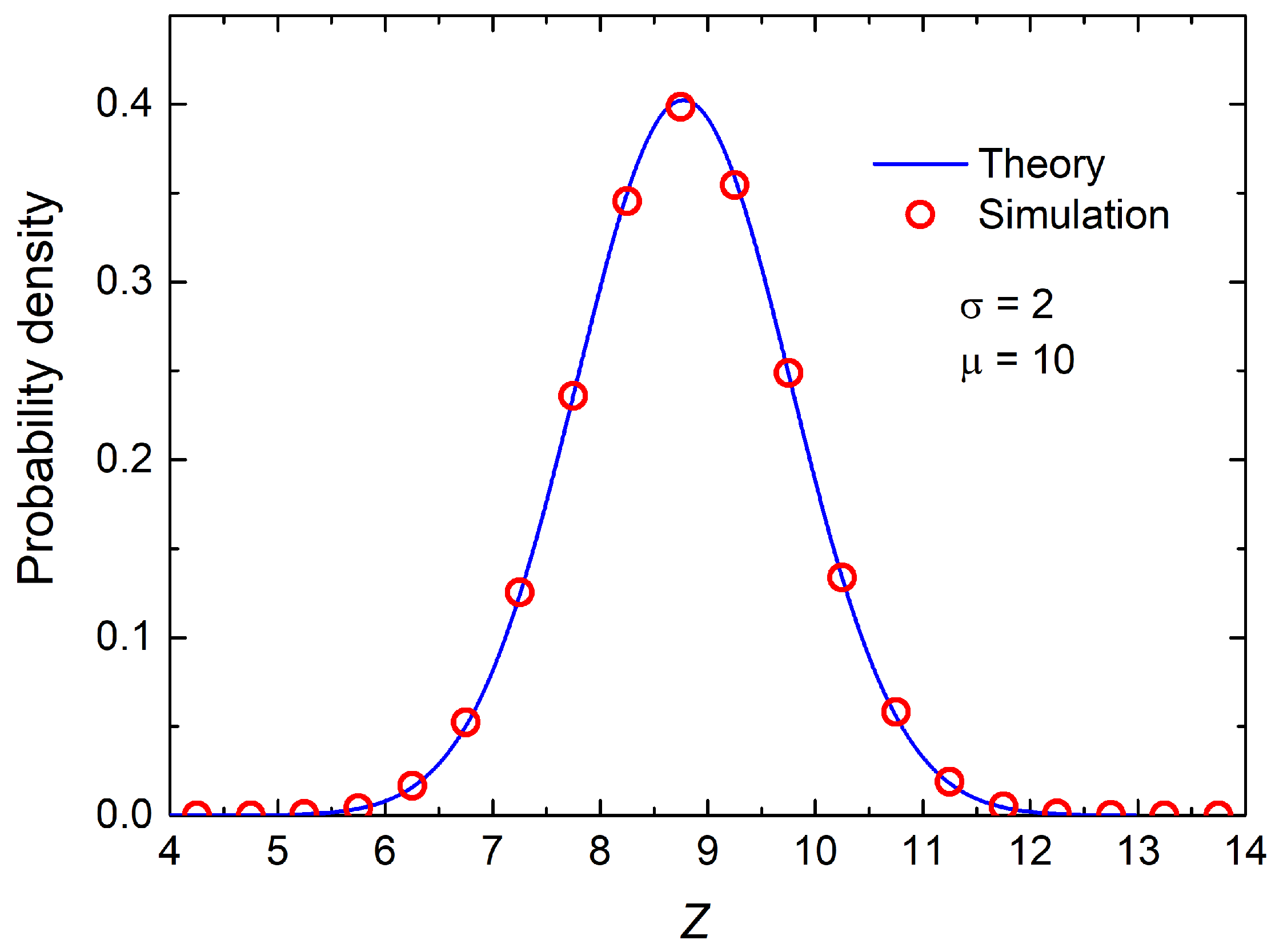The parameter r specifies the seed for random number generation. A total of 2 million random points were used to sample the function. Simulating the non-central chi distribution enables the numerical exploration of how systematic displacements affect a set of independent Gaussian variables. These simulations are particularly useful for studying how the distribution of the magnitude of a multidimensional random vector changes when its mean is varied, while its variance remains constant. The results, displayed in Figure 1 and Figure 2, show a remarkable agreement between the simulated data (red circles) and the theoretical prediction (blue line). 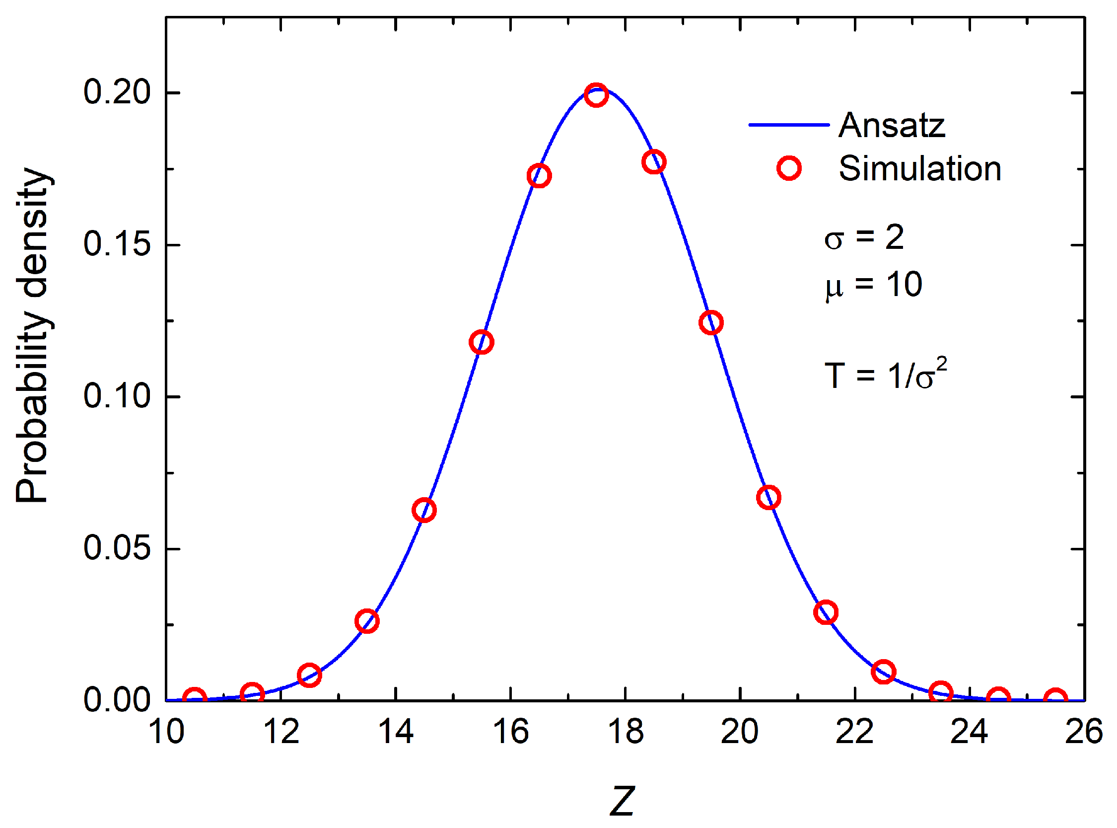In particular, Figure 1 presents the raw distribution from the simulation, which shows a mild but clear asymmetry—a longer right tail—typical of non-central chi distributions.

Figure 2 displays a normalized version of the same variable, where the distribution becomes symmetric around its mean, further reinforcing the interpretation of the non-central component as a shift in the distribution’s origin.

Although the curve in Figure 2 appears visually quite symmetrical at first sight, closer inspection reveals that the right tail (corresponding to higher values of Z) decays less gradually than the left. For example, the decay from $Z=18$ to $Z=22$ on the right is noticeably steeper than the decay from $Z=18$ to $Z=14$ on the left. This observation suggests a slight asymmetry to the right (i.e., a heavier right tail), which is consistent with the behavior of a non-centred or asymmetric distribution, such as a non-central chi distribution or some modified variant thereof.

In contrast, the curve shown in Figure 1 appears to be almost symmetric with respect to its peak (located approximately at $Z=9$). The slopes on either side of the maximum are visually and numerically similar, which is characteristic of a centered distribution, such as the standard normal or a chi distribution with symmetric parameters.

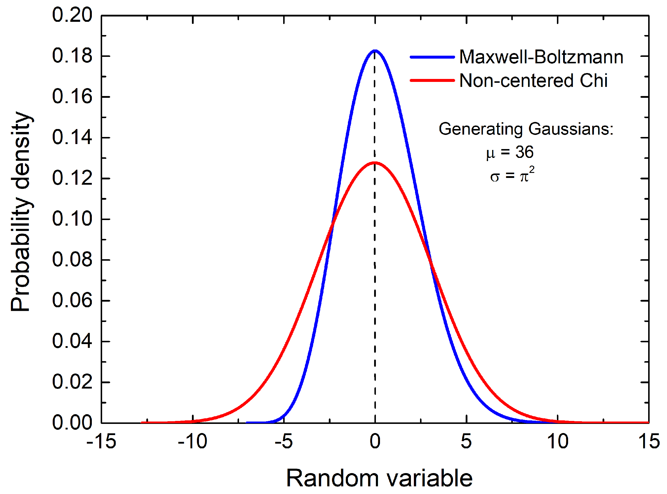
As previously mentioned, besides the parameter $\lambda$, the function also depends on another parameter, T [2]. Figure 3 shows an example, a comparison between the centered chi function with k = 6 degrees of freedom (the generalized Maxwell–Boltzmann distribution function [1]) and the non-centred chi distribution for the same degrees of freedom.

As can be seen, the asymmetry is much more evident in the case of the Maxwell–Boltzmann distribution, whereas in the case of the non-centred chi distribution, it is not immediately apparent from a direct observation of the curve.

As we have already mentioned, our original motivation comes from models related to ideal gas dynamics. So, let us end the section by giving some hints on the physical interpretation of the non-centred chi distribution. From a physical perspective, the non-central chi distribution arises naturally when considering systems in which particles exhibit preferential motion in a specific spatial direction. Unlike the central chi distribution, which describes, for example, the magnitude of particle velocities in an ideal gas in thermal equilibrium, given by the Maxwell–Boltzmann function with $k=3$ degrees of freedom, the non-central version incorporates a displacement parameter. This displacement can be interpreted as the net mean velocity of the particle ensemble, suggesting a system observed from a non-inertial reference frame with respect to the gas.

This displacement parameter does not affect the temperature of the system, which remains proportional to the variance of the underlying Gaussian components. However, it does alter the shape of the distribution, reflecting the anisotropy introduced by the preferential motion. When observed from a reference system moving with that mean velocity, the distribution recovers its centered shape, i.e., it again behaves like a Maxwell–Boltzmann distribution. This property highlights the relevance of the non-centred chi distribution as a useful generalization for describing dynamical systems with directional structure, without involving a change in internal thermal energy.

Thus, this can model, for example, gases with collective motion in a specific direction or situations where a change in the reference frame has been applied to the system, as well as, for example, social and psychological phenomena which involve a non-centred starting point in the model’s expected distribution. To achieve this, independent Gaussian random variables are first generated, all with equal (or comparable) variance and zero mean. Then, a constant $v_i$ is added to each component, representing the system’s collective displacement. This ensures a homogeneous structure in the simulations, facilitating statistical analysis of the results.

3. Main Properties of the Non-Central Chi Distribution

In this section, we present the main features of the class of distributions studied in this paper. Although our primary interest lies in properties related to the intrinsic asymmetry of these functions, a certain form of symmetry can be recovered in the limit. Therefore, we will focus our attention on these limit cases.

3.1. Cumulative Distribution Function

As was written before in Equation (9), the PDF function of the distribution is

$$\widehat{f}(x;T,\lambda ,k)=e^{-T(x^2+{\lambda }^2)/2}{x}^{k/2}T{\lambda }^{1-k/2}{I}_{k/2-1}(x\lambda T).$$

Then, its survival probability function is

$$\widehat{S}(x;T,\lambda ,k)={\int }_x^{\infty }{e}^{-T(x^2+{\lambda }^2)/2}{x}^{k/2}T{\lambda }^{1-k/2}{I}_{k/2-1}(x\lambda T)dx.$$

(10)

If we substitute $L^2=T$, multiply by ${\displaystyle \frac{L^{1-k/2}}{L^{1-k/2}}}$, and group terms, we obtain

$$\widehat{S}(x;L,\lambda ,k)={\int }_x^{\infty }{e}^{-({(Lx)}^2+{(L\lambda )}^2)/2}L{(Lx)}^{k/2}{(L\lambda )}^{1-k/2}{I}_{k/2-1}(LxL\lambda )dx,$$

(11)

so we obtain

$$\widehat{S}(x;L,\lambda ,k)={\displaystyle \frac{1}{{(L\lambda )}^{k/2-1}}}{\int }_x^{\infty }{e}^{-({(Lx)}^2+{(L\lambda )}^2)/2}L{(Lx)}^{k/2}{I}_{k/2-1}(LxL\lambda )dx.$$

(12)

Applying the next change in variables,

$$\left(\begin{array}{c}\gamma =L\lambda \\ y=Lx\\ dy=Ldx\\ x=x\to y(x=x)=Lx=y\\ x\to \infty ;y(x\to \infty )\to \infty \end{array}\right),$$

(13)

we obtain

$$\widehat{S}(y;\gamma ,k)={\displaystyle \frac{1}{{\gamma }^{k/2-1}}}{\int }_y^{\infty }{e}^{-({(y)}^2+{(\gamma )}^2)/2}{(y)}^{k/2}{I}_{k/2-1}(y\gamma )dy$$

(14)

and

$$\widehat{S}(y;\gamma ,k)=Q_{k/2}(\gamma ,y)=Q_{k/2}(\lambda \sqrt{T},x\sqrt{T}).$$

(15)

Knowing that the survival probability function and the cumulative distribution function are complementary, we can express this relationship as

$$\widehat{F}=1-Q_{k/2}(\lambda \sqrt{T},x\sqrt{T}).$$

(16)

Note that, in particular, this implies that the integral of the function $\widehat{f}$ with respect to x in $[0,\infty )$ equals $1.$ Indeed, since $Q_{k/2}(\gamma ,y)\to 0$ as $y\to \infty$ and $Q_{k/2}(\gamma ,0)=1,$ it follows that ${\int }_0^{\infty }\widehat{f}(x;T,\lambda ,k)dx=1$ independently of the values of $T,$ $\lambda$, and $k.$

Also, note that the representation using the Q function is clearly stable for the range used in this paper. It can be easily seen that for ($k\le 50,\lambda \le 20$), there is no numerical problem. The factors $e^{\pm x\lambda T}$ and ${(x/\lambda )}^{k/2}$ could begin to overflow or underflow once k approaches about ${10}^3$ or $\lambda$ approaches about ${10}^2$; in these case, a high-precision implementation of the Q function could be needed.

3.2. Recovery of the Centered Chi Distribution as the Displacement Approaches Zero

Given that Equation (9) is proposed as an ansatz, it is necessary to demonstrate that it recovers the centered chi distribution in the limit of a vanishing displacement.

Since the centered chi distribution is given by [9]

$$f_{\chi }=2^{1-k/2}{T}^{k/2}\mathrm{\Gamma }{(k/2)}^{-1}{x}^{k-1}{e}^{-T{x}^2/2},$$

(17)

it remains to be shown that Equation (9) converges to Equation (17) in the limit $\lambda \to 0$:

$$\underset{\lambda \to 0}{\lim }\widehat{f}=e^{-T{x}^2/2}{x}^{k/2}T\underset{\lambda \to 0}{\lim }{\lambda }^{1-k/2}{I}_{k/2-1}(x\lambda T).$$

(18)

Recall that a modified Bessel function of the first kind is defined as follows:

$$\begin{array}{c}{I}_{k/2-1}(x\lambda T)={\sum }_{j=0}^{\infty }{\displaystyle \frac{1}{j!\mathrm{\Gamma }(k/2+j)}}{\left({\displaystyle \frac{x\lambda T}{2}}\right)}^{2j+k/2-1}=\\ ={\displaystyle \frac{{(x\lambda T)}^{k/2-1}}{2^{k/2-1}\mathrm{\Gamma }(k/2)}}\left[1+{\displaystyle \frac{{(x\lambda T)}^2}{2(k+1)}}+{\displaystyle \frac{{(x\lambda T)}^4}{2·4(k+1)(k+3)}}+\dots \right].\end{array}$$

(19)

Taking the following limits:

$$\underset{\lambda \to 0}{\lim }{I}_{k/2-1}(x\lambda T)=\underset{\lambda \to 0}{\lim }{\displaystyle \frac{{(x\lambda T)}^{k/2-1}}{2^{k/2-1}\mathrm{\Gamma }(k/2)}}\left[1\right]={\displaystyle \frac{{(xT)}^{k/2-1}}{2^{k/2-1}\mathrm{\Gamma }(k/2)}}\underset{\lambda \to 0}{\lim }{\lambda }^{k/2-1}.$$

(20)

If we substitute Equation (20) in Equation (18), we obtain

$$\underset{\lambda \to 0}{\lim }\widehat{f}={\displaystyle \frac{x^{k-1}{T}^{k/2}{e}^{-T{x}^2/2}}{2^{k/2-1}\mathrm{\Gamma }(k/2)}}\underset{\lambda \to 0}{\lim }{\lambda }^{k/2-1}{\lambda }^{1-k/2}={\displaystyle \frac{x^{k-1}{T}^{k/2}{e}^{-T{x}^2/2}}{2^{k/2-1}\mathrm{\Gamma }(k/2)}}.$$

(21)

3.3. Approximation to a Normal Distribution as the Displacement Goes to Infinity

Figure 3 could suggest that the blue curve corresponds to a normal distribution, but in fact it is a non-centred chi distribution when $\lambda$$>>$T. The first step to understanding this is to define the modified Bessel function as z goes to infinity:

$$\underset{z\to \infty }{\lim }{I}_{\alpha }(z)={\displaystyle \frac{e^z}{\sqrt{2\pi z}}}\left(1-{\displaystyle \frac{4{\alpha }^2-1}{8z}}+\dots \right).$$

(22)

Replacing our variables in the previous equation, we obtain

$$\underset{\lambda \to \infty }{\lim }{I}_{k/2-1}(x\lambda T)={\displaystyle \frac{exp(x\lambda T)}{\sqrt{2\pi \lambda xT}}}\left(1-{\displaystyle \frac{k^2+3-4k}{8x\lambda T}}+\dots \right)$$

(23)

We then substitute the following expression into Equation (9):

$$\widehat{f}\mathrm{as}\lambda \to \infty =\sqrt{{\displaystyle \frac{T}{2\pi }}}{x}^{k/2}{\lambda }^{1-k/2}{(\lambda x)}^{-1/2}exp\left(-{\displaystyle \frac{T}{2}}(x^2+{\lambda }^2-2x\lambda )\right)$$

(24)

and simplify to

$$\widehat{f}\mathrm{as}\lambda \to \infty ={\displaystyle \frac{\sqrt{T}}{\sqrt{2\pi }}}{\left({\displaystyle \frac{x}{\lambda }}\right)}^{{\displaystyle \frac{k-1}{2}}}exp\left(-{\displaystyle \frac{T{(x-\lambda )}^2}{2}}\right).$$

(25)

Moreover, as the density is concentrated around $\lambda$ because of the Gaussian exponent, we can also write ${\left({\displaystyle \frac{x}{\lambda }}\right)}^{{\displaystyle \frac{k-1}{2}}}$≈ 1, and finally we obtain the normal approximation

$$\widehat{f}(x;T,\lambda )\approx {\displaystyle \frac{\sqrt{T}}{\sqrt{2\pi }}}exp\left(-{\displaystyle \frac{T{(x-\lambda )}^2}{2}}\right).$$

(26)

Based on this result, we can infer that in the limit $\lambda \to \infty$, the non-centred chi distribution approaches a symmetric form.

Let us now show the rate of convergence of $\widehat{f}$ as $\lambda \to \infty .$ Taking into account the expansion of the modified Bessel function $I_{\alpha }$

$$I_{\alpha }(z)={\displaystyle \frac{e^z}{\sqrt{2\pi z}}}\left(1-{\displaystyle \frac{4{\alpha }^2-1}{8z}}+\mathcal{O}(z^{-2})\right),z\to \infty ,$$

for $\alpha =k/2-1$ and $z=x\lambda T,$ we obtain

$$\widehat{f}(x;k,\lambda ,T)={\displaystyle \frac{\sqrt{T}}{\sqrt{2\pi }}}{e}^{-{\displaystyle \frac{T}{2}}{(x-\lambda )}^2}\left(1-{\displaystyle \frac{4{\alpha }^2-1}{8x\lambda T}}+\mathcal{O}\left({(x\lambda T)}^{-2}\right)\right).$$

Using that ${\displaystyle \frac{k^2+3-4k}{8x\lambda T}}=\mathcal{O}\left({\lambda }^{-1}\right)$ for $\lambda \to \infty ,$ we get $\widehat{f}(x)={\displaystyle \frac{\sqrt{T}}{\sqrt{2\pi }}}{e}^{-\frac{T}{2}{(x-\lambda )}^2}\left[1+\mathcal{O}({\lambda }^{-1})\right].$

4. Applications to Sports Performance Analysis

After establishing the mathematical properties in the previous section, we proceed to illustrate the practical applicability of the non-centred chi distribution by developing a detailed example in the context of sports assessment. Finding studies that explicitly employ the Maxwell–Boltzmann distribution to the context of sports is quite difficult, since this model comes from molecular physics. This distribution has been commonly used to obtain models concerning, for example, air pollutant concentration [17] or zinc concentrations in soil samples [18]. However, there are similar applications for physical models in sports related to fluids or collective influences. Recent studies, such as one on training load modeling in elite athletes [19], have applied multivariate statistical methods similar to those implemented in this work, but they also found no model family to be preferred for athletic performance prediction in their dataset. Regarding the analysis of physical performance, modeling the distribution of the velocities of athletes is a powerful tool. Erdmann et al. [20] analyzed velocity curves in Olympic female skiers, showing differences in the shape of the distribution between elite athletes and lower-level participants, highlighting the informative richness of distributional shapes. In another context, Pałka et al. [21] applied a macroscopic model to the simulation of skier dynamics on slopes, achieving simulated velocities that faithfully reproduced distributions observed in real groups. These studies show the added value of applying physical distributions to real sports data. In this framework, we propose to use the non-centred chi distribution for modeling aggregate athletic performance metrics. The consistency of fits across gender and weight categories, with visibly consistent values of the non-centrality parameter $\lambda$ and temperature-related parameter T, supports the underlying assumption that strength-based outcomes in Olympic weightlifting can be captured through multivariate Gaussian aggregation. In addition, the transition from raw score distributions to a unified probabilistic model facilitates a more appropriate comparison between athletes in different demographic categories.

In addition, the methodology allows for a statistically informed analysis of the dispersion of performance within each category. The different values of T not only reflect the variance in performance results but also suggest possible structural differences in training regimens or levels of specialization between groups.

In order to conduct our analysis, we followed a standard experimental procedure, collecting data and analyzing them in a systematic way.

4.1. Procedure for the Selection and Processing of Experimental Data

To assess the suitability of using the non-central chi distribution, we designed a structured methodology. The evaluation was carried out through the following steps:

• First, in order to assess the normality of the individual test score distributions, we applied the Lilliefors test [22], which is a variation of the Kolmogorov-–Smirnov test adapted for cases where the mean and variance are estimated from the data.
• Second, any sample that did not satisfy the normality assumption according to the Lilliefors test was excluded from further analysis to ensure the robustness of the subsequent steps.
• Third, we assumed that the variances of the retained distributions were similar, and we proceeded analogously to the Ideal Gas Model, generating a synthetic “gas” and determining its corresponding “temperature”.
• Fourth, the individual test scores—those previously validated as normally distributed—were then combined into a composite physical fitness index using the Euclidean norm in k dimensions. This step reflects the aggregation of independent Gaussian variables into a single multivariate measure.
• Finally, the distribution of this aggregated index was fitted to the non-central chi distribution, parameterized by the temperature T and non-centrality parameter $\lambda$, in accordance with Equation (9).

This method was applied in the specific context of the 2019 Weightlifting World Championships. Data on the competition results can be readily accessed online [23]. Our aim is to demonstrate how our methodology enables a more accurate (and arguably fairer) evaluation of the partial results, by aggregating them through our procedure based on the non-central chi distribution.

4.2. Olympic Weightlifting

In this section, the results of the 2019 Weightlifting World Championships will be analyzed [23], which was the last competition before the Tokyo Olympics. It includes the men’s weight categories of −73 kg and −81 kg, and the women’s weight category of −76 kg. In most sports where categories are divided by the competitor’s mass, each category is noted as -pkg to indicate that the competitor’s mass must be less than pkg. This analysis aims to compare variances among different weight categories and between different genders. The data used are shown below; the rest are available in Appendix A.

As is well known, weightlifting competitions consist of two events: the snatch and the clean and jerk. Given the two events in this discipline, the appropriate distribution to apply is the non-centred chi distribution with $k=2$ (non-centred Rayleigh distribution). For the experiment, any subject without scores for either of the lifts was excluded, as well as those whose scores were too low to obtain Gaussian distributions. The fitting and the asymmetry results are detailed in

Table 1. Non-centered chi distribution parameters $\lambda$ and T and skewness $\gamma$ parameter to evaluate the asymmetry of the distributions.

Category	$\mathit{\lambda }$	T	$\mathit{\gamma }$
Male −81 kg	247.18	0.0072	0.2873
Male −73 kg	231.52	0.0045	0.1508
Female −76 kg	165.24	0.0060	0.9338

.

We carried out the ${\chi }^2$ goodness-of-fit test to evaluate the goodness of fit, since it can be used to assess whether a set of categorized data follows a specific theoretical distribution [24]. We obtained that for all examples included in

Table A3. Results of the 2019 Weightlifting World Championships for male −81 kg category. Total (kg) refers to the sum of the Snatch and Clean and Jerk events, Total chi is the proposed measure according to Equation (8), Ranking is the traditional official ranking, and Chi Ranking is the ranking according the proposed methodology. Ties according to the traditional ranking are highlighted in bold.

Name	Snatch (kg)	Clean and Jerk (kg)	Total (kg)	Total Chi	Ranking	Chi Ranking
Lyu Xioayun (CHN)	171	207	378	268.50	1	1
Li Dayin (CHN)	171	206	377	267.73	2	2
Andranik Karapetyan (ARM)	168	199	367	260.43	3	3
Brayan Santiago (COL)	167	196	363	257.50	4	5
Rejepbay Rejepov (TKM)	164	199	363	257.87	4	4
Antonino Pizzolato (ITA)	163	195	358	254.15	6	7
Yunder Nedim (BUL)	157	201	358	255.05	6	6
Andrés Eduardo (ESP)	162	194	356	252.74	8	8
Zacarias Bonnat (DOM)	160	195	355	252.24	9	9
Harrison James Maurus (USA)	152	198	350	249.62	10	10
Mukhammadkodir (UZB)	159	189	348	246.99	11	12
Nico Muller (GER)	157	191	348	247.24	11	11
Ritvars Suharevs (LAT)	154	192	346	246.13	13	13
Victor Getts (RUS)	158	186	344	244.05	14	14
Daniel Godelli (ALB)	155	185	340	241.35	15	15
Juan Felipe Solis Arboleda (COL)	150	189	339	241.29	16	16
Krzysztof Maciej Zwarycz (POL)	150	185	335	238.17	17	17
Emil Moldodosov (KGZ)	153	180	333	236.24	18	18
Erkand Qerimaj (ALB)	151	181	332	235.72	19	20
Ahmed Farooq Ghulam Al-Hussein (IRQ)	147	185	332	236.29	19	19
Alex Bellemarre (CAN)	151	178	329	233.42	21	21
Christian Angel Rodriguez Ocasio (PUR)	147	180	327	232.40	22	22
Arley Mendez Perez (CHI)	150	175	325	230.49	23	23

the ${\chi }^2$ goodness-of-fit test result was below 0.02, which shows a good fit. It can also be observed that there are differences in $\lambda$ between weight categories and genders because strength is highly dependent on body weight. Furthermore, differences in the values of T, in other words, the variances of the distributions (related to their width), were also observed. We have distribution functions depending on the weight and biological sex of the evaluated subjects, unlike the experiments conducted in references [9,12], where the results were age-dependent.

In analyzing the behavior of the non-centered chi distributions across categories, it is important to highlight several relevant aspects. The heavier male categories exhibit larger values of the non-centrality parameter $\lambda$, which is consistent with the physiological expectation of higher absolute strength. Conversely, the lower values for $\lambda$ in the female category reflect the comparatively lower load capabilities while still preserving the structural fit of the distribution. These outcomes reinforce the idea that the distribution model is sensitive to physical characteristics and performance profiles inherent to each demographic.

In terms of variance, represented by the parameter T, we observe wider distributions for the heavier male categories, whereas both the weight and T parameter values for the female −76 kg category are in between the values for the male categories. Regarding the $\gamma$ parameter, which measures the asymmetry of each distribution, we found a significantly larger asymmetry value for the female category compared to the male categories, suggesting more consistent performance among elite lifters in those male groups. This higher asymmetry value for the female category may indicate greater heterogeneity in performance levels, which could be due to a broader competitive range, more diverse physiological profiles, or even potentially less specialization or homogeneity in training.

Regarding practical applications, the classification results generally follow the traditional format (the sum of the snatch and the clean and jerk events). However, it is noted that in the case of ties in the total weight lifted with different results in the events, their competition index, according the proposed methodology, differs, meaning it determines the difficulty of the event and serves as a tiebreaker between two subjects with the same weight lifted. For example, in

Table A1. Results of the 2019 Weightlifting World Championships for female −76 kg category. Total (kg) refers to the sum of the Snatch and Clean and Jerk events, Total chi is the proposed measure according to Equation (8), Ranking is the traditional official ranking, and Chi Ranking is the ranking according the proposed methodology. Ties according to the traditional ranking are highlighted in bold.

Name	Snatch (kg)	Clean and Jerk (kg)	Total (kg)	Total chi	Ranking	Chi Ranking
Jong Sim Rim (PRK)	124	152	276	196.16	1	1
Wangli Zhang (CHN)	118	153	271	193.22	2	2
Aremi Fuentes Zavala (MEX)	107	138	245	174.62	3	3
Neisi Patricia Dajomes Barrera (ECU)	110	135	245	174.14	3	4
Iryna Dekha (UKR)	110	132	242	171.83	5	5
Yeounhee Kang (KOR)	104	131	235	167.26	6	6
Patricia Strenius (SWE)	102	129	231	164.45	7	7
Mariia Vostrikova (RUS)	105	125	230	163.25	8	9
Kristel Ngarlem (CAN)	100	130	230	164.01	8	8
Gulnabat Kadyrova (TKM)	101	123	224	159.15	10	10
Dzina Sazanavets (BLR)	101	120	221	156.85	11	11
Ayumi Kamiya (JAP)	102	118	220	155.97	12	12
Chi-Ling Yao (TPE)	94	122	216	154.01	13	13
Meri Tuuli Linnea Ilmarinen (FIN)	95	118	213	151.49	14	14
Nora Jaeggi (SUI)	91	120	211	150.60	15	15
Quinnie Uzaca Rwahwire (CAN)	92	115	207	147.27	16	16

, for the female −76 kg category, Neisi Patricia Dajomes Barrera and Aremi Fuentes Zavala were tied according the traditional classification ranking), and the same happened with Mariia Vostrikova and Kristel Ngarlem. However, the proposed methodology can be used to provide a more granular ranking (chi ranking), serving as tie breaker for the third and fourth positions and the eighth and ninth, respectively. Another triple tie can be found in

Table A2. Results of the 2019 Weightlifting World Championships for male −73 kg category. Total (kg) refers to the sum of the Snatch and Clean and Jerk events, Total chi is the proposed measure according to Equation (8), Ranking is the traditional official ranking, and Chi Ranking is the ranking according the proposed methodology. Ties according to the traditional ranking are highlighted in bold.

Name	Snatch (kg)	Clean and Jerk (kg)	Total (kg)	Total Chi	Ranking	Chi Ranking
Zhiyong Shi (CHN)	166	197	363	257.61	1	1
Kang Chol O (PRK)	154	193	347	246.91	2	2
Bodzidar Andreev (BUL)	157	189	346	245.70	3	3
Vadzim Likharad (BLR)	154	184	338	239.94	4	4
Briken Calja (ALB)	156	181	337	238.95	5	7
Juhyo Bak (KOR)	151	186	337	239.58	5	5
Julio Ruben Mayora Pernia (VEN)	152	185	337	239.43	5	6
Jeongsik Won (KOR)	153	183	336	238.53	8	8
Chengfei Yuan (CHN)	146	187	333	237.24	9	9
Clarence Cummings Jr (USA)	150	183	333	236.62	9	10
Masanori Miyamoto (JAP)	145	183	328	233.48	11	11
David Sanchez Lopez (ESP)	145	183	328	233.48	11	11
Sergey Petrov (RUS)	153	174	327	231.70	13	15
Max Lang (GER)	147	180	327	232.40	13	13
Triyatno (INA)	145	181	326	231.92	15	14
Doston Yokubov (UZB)	141	180	321	228.65	16	16
Marin Robu (MDA)	149	170	319	226.06	17	17
Rahmat Erwin Abdullah (INA)	144	174	318	225.86	18	18
Maksad Meredov (TKM)	137	178	315	224.62	19	19
Archil Malakmadze (GEO)	142	168	310	219.97	20	20
Kevin David Sandoval Parras (COL)	140	167	307	217.92	21	21
Kakhi Asanidze (GEO)	140	167	307	217.92	21	21
Masakazu Ioroi (JAP)	135	170	305	217.08	23	23
Achinta Sheuli (IND)	135	166	301	213.96	24	24
Tim Kring (DEN)	135	165	300	213.19	25	25

, where Briken Calja, Juhyo Bak, and Julio Ruben Mayora Pernia were in the fifth position according to the traditional ranking and were reordered with the proposed approach. In Table A1, Table A2 and Table A3, we highlight ties according to the traditional ranking in bold. We can observe that there are ties in all three analyzed categories detailed in Appendix A. Thus, ties are much more common than expected, and in all these cases, the proposed new ranking is able to resolve these ties. This is the main contribution regarding the practical application of our methodology. Using this procedure, it is possible to distinguish between situations that are different, although the difference is observed at a more advanced level in the comparison. Furthermore, more superficial aggregation methods are unable to distinguish between these situations.

Thus, this modeling framework not only provides a classification tool but also allows for a better understanding of the underlying dynamics of athlete development and competition structure. This further implies that the proposed statistical modeling not only captures average performance but also provides insight into variability within each group, which could be valuable for training strategies or talent identification. Finally, it is important to remark that, although the model has shown good fitting with the real sports data, no formal uncertainty quantification for the estimated parameters ($\lambda$ and T) was performed in this study. Future work should incorporate this analysis, since it would be valuable in order to assess the robustness and reliability of the model.

5. Conclusions

After some theoretical considerations on the non-centered chi distribution (which has not been extensively studied in the mathematical literature), we presented an application that, in a sense, embodies the canonical phenomenon that this family of distributions is particularly suited to model. In this regard, the introduction of a non-centered version of the chi distribution has proven valuable for describing certain scenarios where more superficial or conventional mathematical modeling could lead to degenerate or misleading results.

Accordingly, as illustrated in the figures, we have demonstrated a notable improvement over the traditional Maxwell–Boltzmann model by employing the modified non-centered chi distribution. However, our research goes beyond merely estimating the probability of encountering a specific index within a population; it also emphasizes the importance of the magnitude of that index, which plays a crucial role in the classification of individuals according to their performance levels.

Moreover, we propose a method for classifying individuals with a normal distribution based on their performance in a specific test—Olympic weightlifting in the context of this study. Yet, a closer examination of our arguments reveals that this methodology is far from restricted to a single context: it can be naturally extended to incorporate other types of physical assessments, thereby supporting the construction of a more comprehensive and nuanced physical fitness index. This approach is especially relevant in cases where simple aggregative statistics (such as the mean) fail to adequately reflect the actual effort required to succeed in a given sport or physical activity.