The Sustainable Allocation of Earth-Rock via Division and Cooperation Ant Colony Optimization Combined with the Firefly Algorithm

Abstract

Optimized earth-rock allocation is key in the construction of large-scale navigation channel projects. This paper analyzes the characteristics of a large-scale navigation channel project and establishes an earth-rock allocation system in phases and categories without a transit field. Based on the physical characteristics of the earthwork and stonework used to design a differentiated transport strategy, a synergistic optimization model is built with economic and ecological benefits. As a solution, this paper proposes a sustainable earth-rock allocation optimization method that integrates the improved ant colony algorithm and firefly algorithm, and establishes a two-stage hybrid optimization framework. The application of the Pinglu Canal Project shows that ant colony optimization via division and cooperation combined with the firefly algorithm reduces the transportation cost by 0.128% compared with traditional ant colony optimization; improves the stability by 57.46% (standard deviation) and 59.09% (coefficient of variation) compared with ant colony optimization through division and cooperation; and effectively solves the problems of precocious convergence and local optimization of large-scale earth-rock allocation. It is used to successfully construct an earth-rock allocation model that takes into account the efficiency of the project and the protection of the ecological system in a dynamic environment.

1. Introduction

In modern engineering construction, the allocation of earth-rock is an important factor that affects the cost of the project and can yield environmental benefits, and at the same time, it is one of the core problems of large-scale navigation channel projects [1]. Earth-rock allocation refers to the construction process under the premise of meeting the excavation schedule and filling schedule, and the comprehensive allocation of earthwork and stonework materials to realize the processes of excavation, mining, filling, transit, processing, and slag disposal [2] to achieve the purpose of improving the direct application rate of excavated materials and reducing the cost of the secondary transfer of earth and stone materials for a rapid and economical construction process [3].

Key to the construction of large-scale navigation channel projects is a scientific and efficient program directly related to the economic cost, construction cycle, and ecological benefits of the project. In the traditional allocation mode, earth-rock allocation mainly focuses on the balance of excavation and filling in earthwork and stonework within the project and the optimization of transportation, mainly by controlling construction costs and the project schedule [4,5,6]. The model is usually situated within the framework of transfer yards to consider the comprehensive allocation of earthwork and stonework, and there is a lack of systematic consideration of the construction schedule. With the increasing prominence of global environmental issues and the growing demand for sustainable allocation in the construction industry, the limitations of this model have been gradually exposed, as the economic benefits of these projects no longer meet the higher requirements of modern society for engineering construction.

Against this background, green earth-rock allocation has emerged. In [7], value engineering theory and the analytic hierarchy process were integrated to explore the construction of a green construction evaluation system based on value engineering. In [8], an adaptive differential evolution algorithm was used to solve a multi-objective optimization model, aiming to derive the optimal material allocation scheme and unify indicator information with value. These studies established a theoretical framework for green earth-rock allocation and provided a systematic methodology for sustainable development in engineering practices.

As the complexity of projects increases, the field of earth-rock allocation has entered an era of algorithmic innovation, with metaheuristics rising to prominence. Ref. [9] proposed an earthwork optimization method based on the ant colony optimization algorithm. By mimicking the process of ant foraging and the mechanism of pheromone trail updating, the algorithm successfully identifies the optimal allocation routes. A hybrid algorithm combining particle swarm optimization and genetic algorithms was employed in [10], leveraging their strong search capabilities to provide cost-effective and efficient allocation solutions for panel rockfill dam projects. The earth-rock allocation problem is analogous to the vehicle routing problem in [11], where a genetic algorithm is used to optimize the allocation path. Ref. [12] presented a study on earthwork allocation using a hybrid algorithm of genetic and taboo search algorithms, which shows superior performance in global search ability and convergence speed. The ant colony algorithm is used to optimize a model in multiple stages in [13], which effectively improves the direct dam placement rate, reduces secondary transportation, and cuts project costs.

This paper analyzes the characteristics of earth-rock allocation for large-scale navigation channel projects from the perspective of economic and environmental benefits. The earth-rock allocation system is established in phases and categories without transfer yards. A sustainable earth-rock allocation model optimization method is proposed, integrating the improved ant colony algorithm and firefly algorithm with a two-phase hybrid optimization framework according to the model characteristics. This method not only fits the model better but also improves the algorithm’s global search capability and stability. It provides a more scientific decision-making basis, a more efficient solution method, and a more environmentally friendly construction program for earth-rock allocation in large-scale navigation channel projects. This promotes the sustainable development of the project. Specifically, the main contributions of this paper are twofold.

(1)

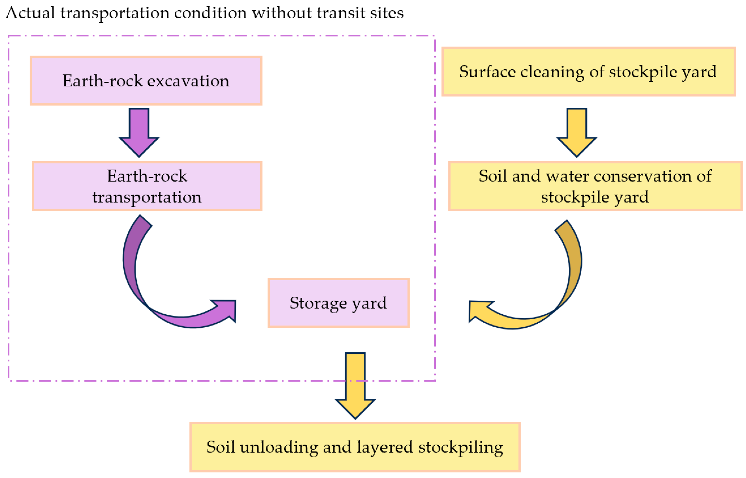
From the perspective of economic and environmental benefits, to analyze the characteristics of large-scale waterway project earth-rock allocation, an allocation model without a transfer yard was established and simplified at the same time to reduce the cost of the transfer yard involved in site leasing, etc. In building the model, we also considered land acquisition project approval time, the project characteristics of the separation of earth-rock allocation independently, and the topsoil, covering a variety of constraints to build a more comprehensive and practical model.

(2)

An optimized sustainable earth-rock allocation model integrating an improved ant colony algorithm and firefly algorithm is proposed, adopting a two-stage hybrid optimization framework. The improved ant colony algorithm is tailored to the characteristics of earth-rock in the improved model to separate and allocate independently, and improves the local search efficiency. The firefly algorithm strengthens global optimization capability, and balances the algorithm’s convergence accuracy and stability through the adaptive parameter adjustment mechanism. The remainder of the paper is organized as follows. Section 2 introduces the earth-rock allocation model. The earth-rock allocation optimization algorithm is proposed in Section 3. Section 4 provides engineering applications, followed by conclusions.

2. Related Works

To further introduce the background of this paper, a detailed account will be provided from the perspectives of earth-rock allocation context, project context, and technical context.

• Earth-rock allocation background

In essence, earthwork allocation refers to the optimization of the spatiotemporal configuration of earthwork resources at construction sites. In the spatial dimension, it is necessary to consider how to reasonably deliver excavated earthwork to required positions or select appropriate spoil sites for stockpiling, while also balancing the planning of transportation routes to reduce costs and minimize time. In the temporal dimension, the sequence of earthwork excavation, transportation, and filling should be arranged according to the construction schedule to ensure seamless phase handover of construction phases and avoid resource wastage.

With the continuous expansion of engineering construction scale and the increasing technical requirements, earthwork allocation has become increasingly complex. On one hand, factors such as geographical conditions, geological status, and surrounding environments at construction sites vary, posing numerous constraints and challenges to earthwork allocation. On the other hand, to achieve sustainable development of engineering construction, multiple factors such as environmental protection, soil and water conservation, and ecological restoration need to be fully considered in earthwork allocation. This has transformed earthwork allocation from a simple engineering technical issue into complex systems engineering involving the economy, the environment, society, and other fields.

2.

Project background

As a major project, the Pinglu Canal and its adjacent Qishi Hub, Youth Hub, etc., demonstrate distinct characteristics in hydrology, sedimentation, and other aspects, posing numerous complex factors to engineering construction. As an important waterway connecting the mainstream of the Xijiang River and the Beibu Gulf, it features a massive construction scale and entails massive earthwork excavation—a challenge that not only poses significant hurdles to construction units in resource allocation but also imposes strict demands on environmental protection and sustainable development. Therefore, an ideal earthwork allocation scheme should strive to balance cost efficiency and construction safety while minimizing ecological impacts.

Against this backdrop, how to use theoretical frameworks and technical means to establish a more scientific and rational earthwork allocation model and adopt algorithmic solutions, so as to achieve the maximum utilization of earthwork resources and the optimization of engineering construction benefits, has become a shared focus of both engineering practice and academic research.

3.

Technical background

With the continuous advancement of numerical simulation technologies and the continuous expansion of engineering application scenarios, metaheuristics algorithms have emerged as core technical tools for solving complex system problems of earthwork allocation, relying on their self-organization, adaptability, and multi-objective optimization characteristics. In research on earthwork resource allocation in civil engineering, along with the significant improvement of engineering applicability of numerical simulation technologies such as computational fluid dynamics and the discrete element method, metaheuristics based on biological swarm intelligence are driving innovative optimizations in earth-rock resource allocation by constructing dynamic optimization models under multi-dimensional constraints.

In [14], a hybrid algorithm combining Gaussian quantum particle swarm optimization and an adaptive genetic algorithm was proposed to address the limitation of balancing global exploration and local refinement in the solution space. In [15], a multi-objective optimal allocation model for urban water resources was designed based on the simulated annealing algorithm, which introduces probabilistic sudden jumps and adopts multi-objective Pareto effective solutions to further improve the simulated annealing algorithm. In [16], a learning-guided dual-population genetic algorithm was proposed, enabling collaborative optimization by storing non-dominated solutions from two populations to achieve knowledge exchange while retaining their independent optimization processes. In [17], an improved heuristic mechanism ACO with four improved mechanisms was proposed, introducing improved pseudo-random transition strategies and dynamic adjustment of pheromone evaporation rates to enhance search efficiency and global search capability, further avoiding local optima.

In [18], an enhanced genetic algorithm tailored to satellite observation constraints was developed for multi-satellite task planning, and empirical results validated its superiority. Through the high abstraction and mathematical modeling of biological swarm intelligence, these algorithms effectively tackle complex optimization problems, demonstrating unique advantages and huge potential in earthwork allocation.

3. Earth-Rock Allocation Model

3.1. Problem Analysis

The earth-rock allocation model is based on the operations research framework of the conventional allocation model, expanding the decision-making dimensions to address the earth-rock characteristics. It inherits basic constraints like supply–demand balance while integrating industry-specific requirements, and it is a specialized extension of the conventional model in the field of civil engineering. The traditional earth-rock allocation system is typically composed of elements such as excavation projects, transfer yards, filling projects, and spoil disposal sites. Among them, the transfer yards fulfill the critical function of “spatiotemporal regulation”. They not only balance the supply–demand fluctuations of earth-rock materials through temporary storage of excavated materials but also optimize transportation routes via secondary trans-shipment. Therefore, the setup of transfer yards is regarded as an important means to tackle complex topography and construction timing mismatches, and their planning is often based on the principle of “minimizing transportation distance”, that is, shortening the single-way transportation distance and reducing the unit transportation cost through multi-level trans-shipment of transfer yards. However, this traditional model has certain limitations in specific scenarios, such as water conservancy hub projects with simultaneous construction, plain-type linear projects, and short-cycle municipal engineering projects. From the dual perspective of natural conditions and economic factors, large-scale navigation channel projects are typically located in flat terrain and geologically stable areas, where excavated materials can be directly backfilled and utilized without relying on secondary methods via transfer yards. At the same time, the construction of transfer yards involves high costs such as site rental, equipment investment, and personnel management. By rationally planning transportation routes and accurately calculating the earthwork volume, the transit link can be avoided, and the economic benefits can be significantly improved. Based on the above background, this paper proposes an earth-rock allocation model without transfer yards, and the simplified process flow is shown in Figure 1, where outside the dotted box is the treatment of surface clearing and soil and water conservation before using the stockpile, and inside the dotted box is the main research content of this paper, i.e., earth-rock allocation without transfer yards, which is directly allocated to the stockpile for soil unloading and soil stacking.

The conventional earth-rock allocation problem considers earthwork and stonework at the same time under an overall framework, reducing the complexity of management and coordination. However, it lacks the flexibility to deploy earthwork and stonework separately, making it difficult to optimize for specific earthwork or stonework. This may lead to unnecessary resource waste in certain aspects. To address this issue, this paper makes the following improvements to the model, as shown in Figure 2, where the purple module is the first improved model, the orange module is the second improved model, and the other color modules have no improvements.

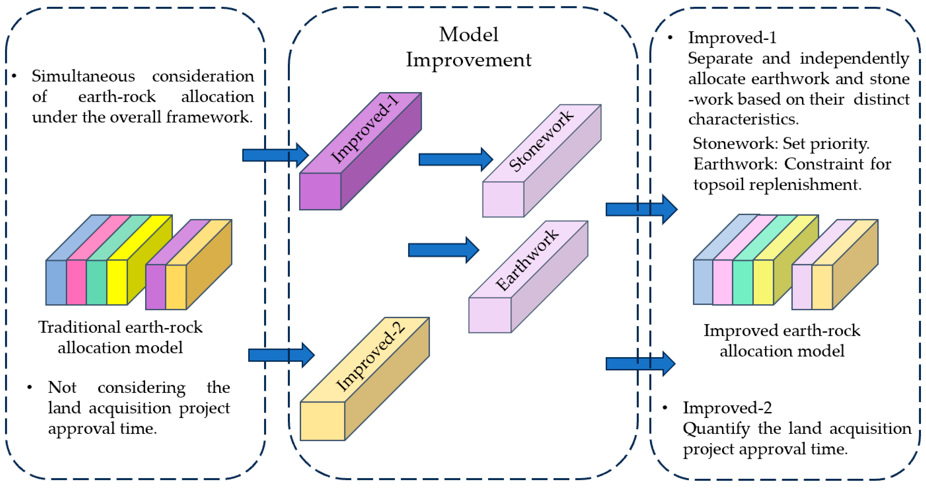
• The model considers independent allocation based on project characteristics, and allocates earthwork and stonework separately, optimizing them according to their specific characteristics. Firstly, given that the unit price of stonework is higher, priority should be given to stonework blending when the transportation distance is shorter. Secondly, according to the soil layer thickness requirements of the relevant standards or specifications for environmental restoration projects, the amount of earthwork is constrained according to the footprint of the stockpile at the later stage of construction, to ensure the effective replenishment of topsoil in the greening area while meeting the needs of the project, thereby promoting environmental protection and ecological restoration.
• Previously, the earth-rock allocation problem did not consider the land requisition project approval timeline, but a reasonable arrangement of the time can reduce the project stagnation period and avoid the waste of manpower, material resources, and other resources caused by timing delays. Therefore, the land requisition project approval time constraint is added to the model to improve the overall efficiency and compliance of the project.

The simplification of the allocation model without transfer yards makes the solution process more efficient and enables quicker identification of the optimal solution among numerous allocation schemes, which greatly broadens the scope of the solution space. At the same time, to avoid the omission of key factors that may be caused by the simplified model, this paper adds the aforementioned constraints to the model in addition to the necessary constraints. This ensures that the model overcomes deviations triggered by simplification while pursuing efficiency and accuracy, making the no-transfer-yards model highly feasible and scientific. It thus provides a more accurate and practical solution for the earth-rock allocation in waterway engineering.

3.2. Modeling

According to the above analysis of model characteristics, consideration of deployment from small to large, and the principle of proximity, that is, the priority configuration of independent and smaller-capacity stockpiling sites, the earth-rock quantity of the nearest excavation section is prioritized for stockpiling, and the whole process of calculating the minimum earth-rock allocation costs is constructed as an objective function:

$$M=\min \left\{{\displaystyle {\sum }_{t=1}^k\left[{\displaystyle {\sum }_{i=1}^{n_W}{\displaystyle {\sum }_{j=1}^{n_T}{C}_{W_i{T}_j}^{\left(t\right)}{X}_{W_i{T}_j}^{\left(t\right)}}}+{\displaystyle {\sum }_{i=1}^{n_W}{\displaystyle {\sum }_{j=1}^{n_T}{C}_{W_i{T}_j}^{\prime \left(t\right)}{X}_{W_i{T}_j}^{\prime \left(t\right)}}}+{\displaystyle {\sum }_{i=1}^{n_W}{\displaystyle {\sum }_{j=1}^{n_T}{U}_{ij}\left(X_{W_i{T}_j}^{\left(t\right)}+X_{W_i{T}_j}^{\prime \left(t\right)}\right)}}\right]}\right\}$$

(1)

where M is the objective function, i.e., the total allocation cost in CNY; $C_{W_i{T}_j}^{\left(t\right)}$ is the unit price for the allocation of earthworks for excavation project ($W_{\mathrm{i}}$) and fill project ($T_j$) at time t, in CNY/m³; $X_{W_i{T}_j}^{\left(t\right)}$ is the volume of transported cubic meters of earthworks to be mobilized for excavation project ($W_{\mathrm{i}}$) and fill project ($T_j$) at time t, in m³; $C_{W_i{T}_j}^{\prime \left(t\right)}$ is the unit price for the allocation of stonework for excavation project ($W_{\mathrm{i}}$) and fill project ($T_j$) at time t, in CNY/m³; $X_{W_i{T}_j}^{\prime \left(t\right)}$ is the volume of transported cubic meters of stonework to be mobilized for excavation project ($W_{\mathrm{i}}$) and fill project ($T_j$) at time t, in m³; $U_{ij}$ is the cost of soil and water conservation, in CNY.

3.3. Constraints

①

Balance constraint for supply and reception:

$${\displaystyle {\sum }_{i=1}^{n_W}\left(X_{W_i{T}_j}^{\left(t\right)}+X_{W_i{T}_j}^{\prime \left(t\right)}\right)}=S_{T_j}^{\left(t\right)}$$

(2)

The sum of the earthwork and stonework excavated for the excavation project ($W_i$) equals the total (${S^{(t)}}_{T_j}$) for fill project ($T_j$) at time t.

$$S_{T_j}^{\left(t+1\right)}=S_{T_j}^{\left(t\right)}+{\displaystyle {\sum }_{i=1}^{n_W}\left(X_{W_i{T}_j}^{\left(t+1\right)}+X_{W_i{T}_j}^{\prime (t+1)}\right)}$$

(3)

${S^{(t+1)}}_{T_j}$ is the total amount of stockpiles for fill project ($T_j$) at time t + 1.

②

Capacity constraint for stacking:

$${\displaystyle {\sum }_{t=1}^k{\displaystyle {\sum }_{i=1}^{n_W}\left(X_{W_i{T}_j}^{\left(t\right)}+X_{W_i{T}_j}^{\prime \left(t\right)}\right)}}\le V_{T_j}$$

(4)

The sum of the excavated quantities of earthwork and stonework for the excavation project ($W_i$) does not exceed the maximum stockpile ($V_{T_j}$) for fill project ($T_j$) at time t.

③

Time constraint for land requisition project approval:

$$Q_c={\left(q_{tj}\right)}_{4\ast n}$$

(5)

$$q_{tj}=\left\{\begin{array}{c}0, \mathrm{Quarter} \left(\mathrm{t}\right) \mathrm{in} \mathrm{fill} \mathrm{project} \left(\mathrm{j}\right) \mathrm{is} \mathrm{undeployable}\\ 1,\mathrm{Quarter} \left(\mathrm{t}\right) \mathrm{in} \mathrm{fill} \mathrm{project} \left(\mathrm{j}\right) \mathrm{is} \mathrm{deployable}\end{array}\right.$$

(6)

where $Q_c$ (Quarters Constraint) is a constraint on the allocation of n fill projects in the four quarters.

④

Constraint for stonework near priority:

$$P\left(\mathrm{S}\right)={\displaystyle \frac{w(S)}{D}}\times U(S)\ge {\displaystyle \frac{1}{D}}\times U(E)=P(E)$$

(7)

$P\left(\mathrm{S}\right)$ and $P\left(\mathrm{E}\right)$ represent the probability of transportation of stonework and earthwork ($P\left(\mathrm{S}\right),P\left(\mathrm{E}\right)\in \left[0,1\right]$), $U(S)$ and $U(E)$ represent the unit price of transportation of stonework and earthwork, and the priority weight of stonework is $w(S)(w(S)\ge 1)$. When the transportation distance D (D > 0) is closer, the stonework with a higher unit price of transportation is preferentially allocated.

⑤

Constraint for topsoil overlay:

$${\displaystyle {\sum }_{i=1}^{n_W}{X}_{W_i{T}_j}^{\left(t\right)}}\ge h\ast k_j\ast A_{tj}\left(t=4\right)$$

(8)

For effective subsequent topsoil overlays, an average thickness of earthwork cover of h is required in the fourth quarter, where the loose fill volume factor is $k_j$ and the filled project ($T_j$) footprint is $A_{tj}$.

⑥

Zero constraints for excavation quantity at the end of allocation:

$$S_{W_i}^{\left(t\right)}+S_{W_i}^{\prime \left(t\right)}-{\displaystyle {\sum }_{j=1}^{n_T}\left(X_{W_i{T}_j}^{\left(t\right)}+X_{W_i{T}_j}^{\prime \left(t\right)}\right)}=0$$

(9)

At the end of the allocation, the planned volume of excavated earthwork ($S_{W_i}^{\left(t\right)}$) and stonework ($S_{W_i}^{\prime \left(t\right)}$) should be completed.

⑦

Constraint for non-negative variables:

$$x_{ij}\ge 0(\forall i,j)$$

(10)

x_ij represents any variable in this model, such as allocation quantity, transfer probability, distance, cost, etc. All variables are non-negative.

4. Earth-Rock Allocation Optimization Algorithm

4.1. Evolution from ACO to DC-ACO

According to Wolpert’s No Free Lunch theorem, no optimization algorithm can universally surpass others on all problems [19]. For earth-rock allocation problems, advanced algorithms like the Reptile Search Algorithm and the Red Fox Optimizer have their limitations. The Reptile Search Algorithm’s fixed-step local search strategy struggles with non-convex constraints caused by soil parameter fluctuations [20,21,22]. The Red Fox Optimizer, with its empirically set objective function weights, has difficulty balancing multi-objective conflicts in earthwork allocation, which demands explicit resolution of the Pareto front [23,24]. Such limitations may lead to infeasible solutions in ecologically sensitive engineering projects.

Selecting the ant colony optimization for earth-rock allocation in large-scale navigation channel projects is due to its multi-faceted adaptability. It can effectively handle discrete decision-making problems in earth-rock allocation, such as choosing allocation routes and assigning supply and demand nodes. Its robustness and distributed computing capabilities enable optimization under complex constraints like construction schedule and transportation capacity. Moreover, its role-based allocation mechanism aligns closely with the model requirements. The earth-rock allocation model in this study requires separate allocation of earthwork and stonework. The improved ant colony algorithm’s role-based allocation mechanism fits well with the model. Different ant roles can be assigned to handle earthwork or stonework allocation. They follow their rules and pheromone guidance to independently and collaboratively allocate different earthwork and stonework types, enhancing the rationality of the allocation plan.

4.1.1. ACO

Ant colony optimization (ACO) is an intelligent optimization algorithm developed by simulating the foraging behavior of ants. Through extensive research, biologists have discovered that ant colonies leave a special substance—pheromones—on the paths they traverse during the foraging process, which serves as a cue for other ants to find food.

The succeeding ants determine their forward direction according to the pheromone concentration, and the pheromone volatilizes over time; both the path length and residual pheromone amount significantly influence ants’ choice. The more ants traverse a path within a given time, the higher the probability of ants choosing the path, while the pheromone concentration is strengthened, prompting more ants to follow suit, thus realizing a positive feedback information learning mechanism to quickly find the shortest path from the food source to the nest [25].

By simulating the pheromone accumulation and updating mechanism of ant colony foraging, the ant colony algorithm can effectively deal with discrete decision-making problems such as allocation path selection and source and destination nodes in earth-rock allocation, and its distributed computing capability can be used to find the optimal solution under complex constraints such as construction schedule and transportation capacity. Considering the differences in the allocation requirements of earthwork and stonework in actual projects, and the need to meet multiple constraints such as earth-rock balance, transportation capacity, etc., the traditional ant colony algorithm has limitations such as low optimization efficiency in dealing with this kind of differentiated allocation task.

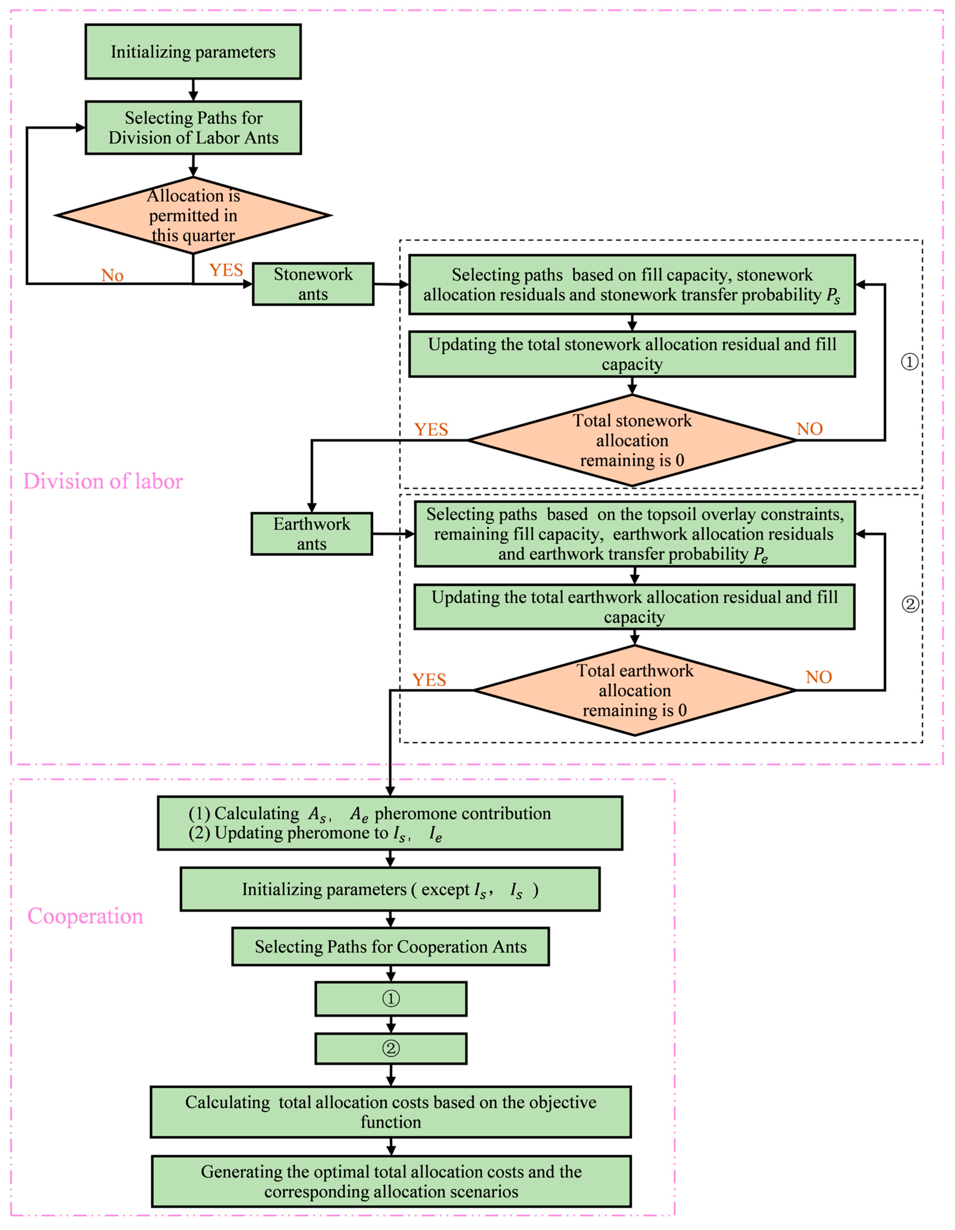
4.1.2. DC-ACO

In ant colony optimization, the ants consider the pheromone concentration of the path from the previous node to the current node as well as the heuristic information of the current node when choosing the next node, and the algorithm performs pheromone updating after the ants’ path selection is completed, which usually relies on the successful paths (which refer to the lower total allocation cost) only to increase the pheromone concentration, and the pheromone is shared by all the ants, so that when a path starts to be selected by too many ants, other potential paths may be ignored, leading to premature convergence. To address this issue, the ant colony is often grouped to perform the search. However, if the two colonies have different convergence speeds and operate independently, the final results may fluctuate significantly, which in turn affects the quality of the final solution.

Based on this, to further meet the requirement of separate allocation for earthwork and stonework in the earth-rock allocation model, and to improve the optimization performance of the algorithm in complex scenarios, this study proposes the division and cooperation ant colony optimization, DC-ACO. The core of the algorithm is to assign different “roles” to the ants, i.e., stonework ants $\left(A_s\right)$ and earthwork ants $\left(A_e\right)$, to perform the allocation tasks of stonework and earthwork, respectively, based on the symmetrical design of the search rules, and then update the pheromone left behind after the search of $A_s$ and $A_e$, respectively, to the transfer probability of the total ant colony in the next cycle, so as to generate the final allocation scheme. This improvement not only fully leverages the group intelligence advantage of ACO but also achieves more refined optimization for the characteristics of earth-rock allocation, and effectively enhances the rationality and feasibility of the scheme.

Updated transfer probabilities:

$$I_s=P_s\times S_{{\tau }_s}$$

(11)

$$I_e=P_e\times S_{{\tau }_e}$$

(12)

Among them,

$$S_{{\tau }_s}=\left(1-\gamma \right)\times \overline{S_{{\tau }_s}},S_{{\tau }_e}=\left(1-\gamma \right)\times \overline{S_{{\tau }_e}}$$

(13)

$${\tau }_s={\displaystyle \frac{Q}{f_s}},{\tau }_e={\displaystyle \frac{Q}{f_e}}$$

(14)

$P_s\left(P_e\right)$ is the stonework (earthwork) original transfer probability, $\overline{S_{{\tau }_s}}\left(\overline{S_{{\tau }_e}}\right)$ is the pheromone, $S_{{\tau }_s}\left(S_{{\tau }_e}\right)$ denotes the pheromone after volatilization treatment for $\overline{S_{{\tau }_s}}\left(\overline{S_{{\tau }_e}}\right)$, while ${\tau }_s\left({\tau }_e\right)$ is the pheromone contribution to each path calculated by $A_s\left(A_e\right)$ based on the fitness, Q is the pheromone strength, $\gamma$ is the proportion of pheromone volatilization rate, $f_s\left(f_e\right)$ is a random number extracted from a uniform distribution, serving as the fitness of each simulated stonework (earthwork) ant.

To address the issue of single-pheromone updating, the pheromone updating mechanism is dynamically adjusted, closely linked to the allocation distance and the allocation unit price. Since the unit price is affected by the distance from the source node (src) to the target node (dest), both distance and allocation unit price are integrated into the transfer probability calculation. According to the principle of separating project characteristics and independent allocation, the priority factor is introduced into the stonework allocation process. By adjusting the priority weight $w_s$ of stonework, preferential allocation can be achieved when the transportation distance is shorter. The transfer probabilities of stonework and earthwork are as follows:

$$P_s\left(src\right)=sum{\left({\displaystyle \frac{w_s}{d\left(dest\right)}}\times u_s\left(dest\right)\right)}^{\alpha }$$

(15)

$$P_e\left(src\right)=sum{\left({\displaystyle \frac{1}{d\left(dest\right)}}\times u_e\left(dest\right)\right)}^{\alpha }$$

(16)

The transfer probabilities (11) and (12) are transformed into:

$$I_s\left(src\right)=P_s\left(src\right)\times S_{{\tau }_s}\left(dest\right)$$

(17)

$$I_e\left(src\right)=P_e\left(src\right)\times S_{{\tau }_e}\left(dest\right)$$

(18)

where d is the distance from the source node to the destination node, $u_s$ ($u_e$) is the unit price of stonework (earthwork) allocation, and $S_{{\tau }_s}\left(dest\right)\left(S_{{\tau }_e}\left(dest\right)\right)$ is the specific pheromone intensity extracted from each path’s pheromone after updating. The process of DC-ACO is shown in Figure 3 (the pseudocode of DC-ACO is shown in Algorithm A1, Appendix A), where the top half of the figure shows $A_s$ and $A_e$ chosen based on the information division of labor, and the bottom half shows the total colony choosing collaboratively based on the updated information.

4.2. Evolution from DC-ACO to DC-FACO

For the earth-rock allocation problem, DC-ACO becomes a preferred choice for solving the earth-rock allocation by virtue of its unique ability to handle discrete variables, adapting to complex constraints, and a role-splitting allocation mechanism that aligns with the model requirements.

However, the optimization of the algorithm performance is a continuous exploration process. Although DC-ACO effectively improves the global search capability and convergence efficiency in the earth-rock allocation through symmetric logic and a division-of-labor synergy mechanism, its solution stability still has limitations. The algorithm relies on the accumulation and updating of pheromones to guide the search direction, and when dealing with large-scale complex allocation scenarios, the dynamic balance of the pheromone is easily disrupted by the local optimal paths, which leads to large fluctuations in the algorithm’s solution results. Especially when the scale of allocation is enlarged and the number of constraints increases, the solution space exploration of ACO has randomness and repetitiveness, which makes it difficult to ensure that a stable and high-quality solution can be output in each run.

4.2.1. FA

The firefly algorithm (FA) is a stochastic optimization algorithm constructed by simulating the luminescence behavior of fireflies in nature, which shows good stability and adaptability in solution space exploration by virtue of the dynamic regulation of fluorescein and the individual attractiveness mechanism. The algorithm can continuously optimize the solution quality globally by simulating the group interaction behavior of fireflies, and prevent the algorithm from getting stuck in local optima by dynamically adjusting the search step size and direction.

The reason why fireflies are attracted to each other depends on two elements, i.e., their brightness and attractiveness. The brightness of the fluorescence emitted by fireflies depends on the objective function value at their location, and the higher the brightness, the better the location, i.e., the better the objective function value [26].

The core of the FA lies in its position update formula, an update mechanism that combines the current firefly’s position, brightness-based attractiveness, distance, and random perturbations:

$$x_i=x_i+\beta e^{-\gamma r^2}\left(x_j-x_i\right)+\alpha \epsilon$$

(19)

where $\beta e^{-\gamma r^2}$ denotes the attraction of fireflies to other brighter fireflies, enabling efficient local exploration. $\alpha \epsilon$ denotes a random factor that prevents the algorithm from falling into a local optimal solution and enhances exploration capability.

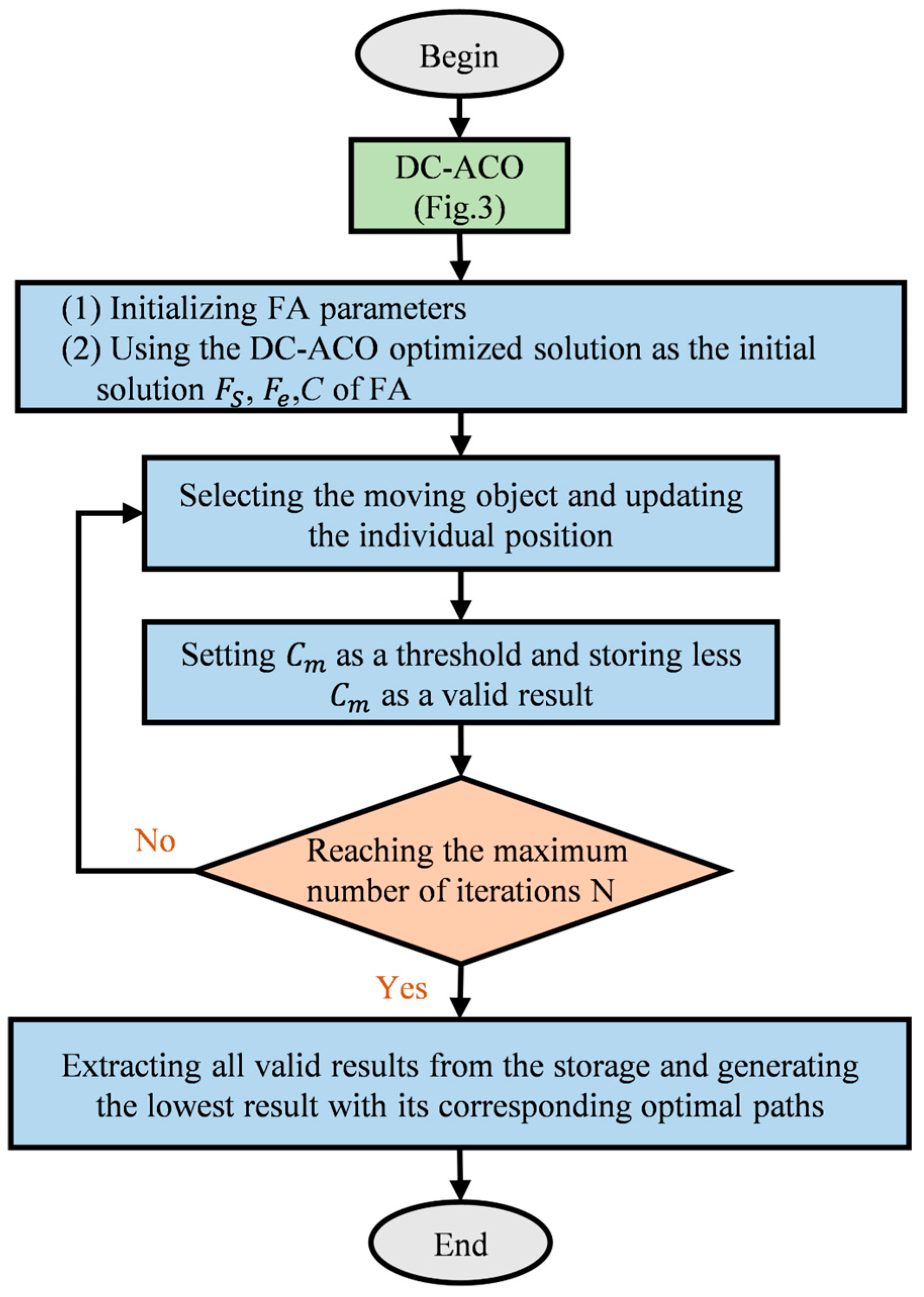
4.2.2. DC-FACO

Therefore, combining the firefly algorithm (FA) with the division and cooperation ant colony optimization (DC-ACO) creates a hybrid algorithm (DC-FACO) that leverages the complementary strengths of both. The high-quality initial solutions provided by DC-ACO effectively guide the FA to avoid initial search blindness and accelerate convergence toward the global optimum. Meanwhile, FA’s stable self-adaptive optimization capability enables fine-grained adjustment of these initial solutions, reducing result volatility.

Using DC-ACO’s optimized solution as the initial input for FA,

$$F_S={\left[S^{\ast }{S}^{\ast }\cdots S^{\ast }\right]}_{1\ast 1\ast 1\ast N}$$

(20)

$$F_E={\left[E^{\ast }{E}^{\ast }\cdots E^{\ast }\right]}_{1\ast 1\ast 1\ast N}$$

(21)

$$C={\left[C_{\min }{C}_{\min }\cdots C_{\min }\right]}_{N*1}$$

(22)

where $S^{\ast },E^{\ast },C_{\min }$ denote the optimal stonework allocation scheme, optimal earthwork allocation scheme, and minimum cost obtained by DC-ACO, N denotes the number of fireflies, $F_S\left(F_E\right)$ denotes the location of fireflies for stonework (earthwork) allocation, and C denotes the cost of each firefly.

4.2.3. DC-FACO-Based Earth-Rock Allocation Process

The specific process of DC-FACO for earth-rock allocation is as follows.

Step 1: Initialization. Set the parameters of the ant colony optimization, the number of allocation endpoints, the number of quarters, the total number of ants $m_a$, the number of stonework (earthwork) ants $m_s\left(m_e\right)$, the number of iterations N, the pheromone importance α, the heuristic function importance β, and the pheromone evaporation rate γ. Initialize the allocation data of earthwork and stonework volumes, the matrix of the allocation scheme as well as the pheromone matrix for the ants’ paths, and the allocation matrices of the stonework cubes and the earthwork cubes, and set the initial minimum cost to infinity.

Step 2: Division-of-labor ant path selection. Perform path selection based on land requisition project approval time, each available fill capacity, and the dynamically adjusted transfer probability (Equation (15)), and generate four-quarter stonework allocation plans, updating every fill capacity, and the total residual of stonework allocation until there is no remaining planned stonework volume. Similarly, at the end of the allocation, the same strategy is used for path selection based on the remaining fill capacities and topsoil overlay constraints, updating earthwork residuals until planned earthwork volumes are fully allocated. After pheromone concentration evaporation, calculate and update pheromone contributions separately.

Step 3: Collaborative ant path selection. Initialize the allocation data and allocation scheme matrix of stonework and earthwork. The total ant colony performs path selection based on the updated Is and Ie, the same strategy is used until there is no surplus of the total allocation of stonework and earthwork, and the total allocation cost is calculated. Iterate; if the maximum number of iterations N is reached, proceed to step 4; if not, go back to step 2.

Step 4: Ant colony optimal path output. Compare the minimum allocation cost generated by each iteration, take the smallest value as the global optimal allocation cost, and record the corresponding stonework and earthwork allocation plans for the four quarters.

Step 5: Firefly initialization. Set the number of fireflies $m_f$, the number of iterations N, the perturbation factor ${\alpha }^{\prime }$, the attraction factor ${\beta }^{\prime }$, and the decay rate factor ${\gamma }^{\prime }$, and use the optimized solution as the initial solution $F_S,F_e,\mathrm{C}$ of the firefly algorithm.

Step 6: Select moving object and update position. Compare the cost of each pair of fireflies; if the price of firefly f1 is higher than f2, then f1 will move towards f2. Select the object and update its position according to Equation (19).

Step 7: Cost comparison. Store the results of each run (total price of allocation), set the global optimal allocation price recorded by the ant colony to the threshold $C_m$, and if the current price is less than $C_m$, store it in table T. Iterate; if the maximum number of iterations N is reached, proceed to step 8; if not, go back to step 6.

Step 8: Optimal path output. Extract all valid results (less than $C_m$) from T and output the minimum total price of the allocation and its corresponding stonework and earthwork allocation scheme.

The specific allocation process is shown in Figure 4 (the pseudocode of DC-FACO is shown in Algorithm A2, Appendix A), where the green box represents the workflow of Figure 3. Subsequently, the optimal solution obtained by DC-ACO is used as the initial solution of the firefly algorithm, and the optimization search is continued to obtain the final optimal solution.

5. Engineering Applications

5.1. Engineering General Situation

Land Canal begins at the mouth of Pingtang River in Hengzhou City, Nanning, in the Xijiang River main stream in the Xijin Reservoir area, crosses the watershed of Shaping River and Jiuzhoujiang township, a tributary of Qinjiang River, and enters the waters of Qinzhou Harbor in the Gulf of Beibu along the main stream of Qinjiang River to the south by Lingshan County, Qinzhou City, in the town of Luhu. The scope of this waterway project is the waterway construction NO.HD7 bidding section, constructed according to the standard of a Class I waterway. The main design content includes the general plan of the waterway, slope and bank revetment works, soil and water conservation, earth-rock stockpiling yards, large-scale temporary works, road and bridge works, environmental protection, navigational marking systems, landscape greening, and so on. The project volume of this section is large: the total volume of earthwork is 21,411,600 m³ (including 6,287,800 m³ of land-based stonework excavation and 9,071,200 m³ of land-based earthwork excavation), and the length of the navigation channel is 6600 m. The construction work is long and includes many lines, and it is difficult to organize the construction to ensure that the target of the construction period can be achieved and to reduce the cost of the earth-rock allocation, which is the critical focus of this section.

According to the design drawings and relevant survey data, the amount of earth-rock excavation and fillings in each region of the project in 2024 is calculated. The total amount of planned stonework excavation is $340.44\times {10}^4$ m³, the total amount of earthwork excavation is $339.01\times {10}^4$ m³, and the 12 fillings are expressed by $K_i$. The parameter datasheet is shown in

Table 1. Parameter datasheet.

	Fillings	K1	K2	K3	K4	K5	K6	K7	K8	K9	K10	K11	K12
Names
Occupany area (hm2)		2.2	8.3	12.4	6.2	3.5	9.7	6.5	1.5	4.1	63.7	10.2	89.1
Average transportation distance (km)		0.2	0.6	0.9	0.4	0.9	0.3	0.4	0.4	0.2	4.6	4.8	5.1
Design capacity (million m3)		12.7	53.7	76.7	36.1	10.2	72.6	31.1	4.9	17.6	877.4	506.0	453.9

, where the first row lists the numbering of fillings, and the following three rows show the parameters of the occupancy area, average transportation distance and maximum design capacity of each of the twelve allocation sites.

According to the filling approval form date, the allocation status of the fillings is summarized in

Table 2. Quarterly allocation situation.

	Fillings	K1	K2	K3	K4	K5	K6	K7	K8	K9	K10	K11	K12
Names
Q1		0	0	0	1	1	0	0	1	1	1	0	0
Q2		0	0	0	1	1	0	0	1	1	1	1	1
Q3		1	1	1	1	1	1	1	1	1	1	1	1
Q4		1	1	1	1	1	1	1	1	1	1	1	1

, where the first row is the filling numbering, and the following four rows show the allocation of these 12 stockyards in each of the four quarters, with 0 being non-allocation.

According to the regulations, the average thickness of topsoil stripping is 0.3 m, the volume factor for earthwork fill is 1.08, and the volume factor for stonework backfill is 1.31. The unit price per cubic meter of topsoil overlay is obtained by the ratio of the total environmental protection cost to the total planned volume of earth-rock, which is about CNY 26.34/m³. The unit price of stonework transportation is as follows: CNY 14.76/m³ within 1 km; above 1 km, for every additional 100 m distance, the comprehensive unit price increases by CNY 0.1308/m³. The unit price of earthwork transportation is as follows: CNY 10.64/m³ within 1 km; above 1 km, for every additional 100 m distance, the comprehensive unit price increases by CNY 0.109/m³. The details are shown in Figure 5, where the horizontal axis represents the transportation distance, the vertical coordinate represents the transportation unit price, the blue dashed line is the unit price for stonework allocation, and the orange dashed line is the unit price for earthwork allocation.

5.2. Comparative Analysis of the Results of Different Algorithms

Taking the lowest total cost of earthwork and stonework allocation and topsoil overlay as the optimization objective, according to the given relevant datasets and constraints, the two are jointly optimized, and the optimal allocation scheme is obtained by solving and comparing using ACO, DC-ACO, and DC-FACO algorithms, respectively, as shown in

Table 3. Solving the optimal allocation scheme based on ACO.

Quarters	Q1		Q2		Q3		Q4
Fillings	S	E	S	E	S	E	S	E
K1	0.0000	0.0000	0.0000	0.0000	7.4100	4.5730	0.0000	0.7170
K2	0.0000	0.0000	0.0000	0.0000	47.4900	3.5101	0.0000	2.6999
K3	0.0000	0.0000	0.0000	0.0000	51.2600	21.4117	0.0000	4.0283
K4	25.2300	8.8699	0.0000	0.0000	0.0000	0.0000	0.0000	2.0001
K5	8.5200	0.5525	0.0000	0.0000	0.0000	0.0000	0.0000	1.1275
K6	0.0000	0.0000	0.0000	0.0000	13.8400	18.0595	37.5600	3.1405
K7	0.0000	0.0000	0.0000	0.0000	0.0000	0.7080	26.1800	2.1060
K8	3.5300	0.3766	0.0000	0.0000	0.0000	0.0000	0.0000	0.4967
K9	14.3300	0.7437	0.0000	0.0000	0.0000	0.0000	0.0000	1.3132
K10	68.3800	74.2098	36.7000	84.7526	0.0000	36.4902	0.0000	34.9631
K11	0.0000	0.0000	0.0000	0.0000	0.0000	0.0000	0.0000	3.2918
K12	0.0000	0.0000	0.0000	0.0000	0.0000	0.0000	0.0000	28.8684

,

Table 4. Solving the optimal allocation scheme based on DC-ACO.

Quarters	Q1		Q2		Q3		Q4
Fillings	S	E	S	E	S	E	S	E
K1	0.0000	0.0000	0.0000	0.0000	10.0900	1.8930	0.0000	0.7170
K2	0.0000	0.0000	0.0000	0.0000	47.2300	3.7601	0.0000	2.6999
K3	0.0000	0.0000	0.0000	0.0000	61.3000	11.3717	0.0000	4.0283
K4	31.5700	2.5299	0.0000	0.0000	0.0000	0.0000	0.0000	2.0001
K5	8.3000	0.2725	0.0000	0.0000	0.0000	0.0000	0.0000	1.1275
K6	0.0000	0.0000	0.0000	0.0000	1.3800	0.4895	67.5900	3.1405
K7	0.0000	0.0000	0.0000	0.0000	0.0000	0.0000	27.7600	2.1060
K8	3.5350	0.3716	0.0000	0.0000	0.0000	0.0000	0.0000	0.4967
K9	14.8600	0.1137	0.0000	0.0000	0.0000	0.0000	0.0000	1.3132
K10	61.2350	81.4648	5.0900	84.7525	0.0000	67.2382	0.0000	34.9631
K11	0.0000	0.0000	0.0000	0.0000	0.0000	0.0000	0.0000	3.2918
K12	0.0000	0.0000	0.0000	0.0000	0.0000	0.0000	0.0000	28.8684

and

Table 5. Solving the optimal allocation scheme based on DC-FACO.

Quarters	Q1		Q2		Q3		Q4
Fillings	S	E	S	E	S	E	S	E
K1	0.0000	0.0000	0.0000	0.0000	10.5300	1.4530	0.0000	0.7170
K2	0.0000	0.0000	0.0000	0.0000	47.4900	3.5101	0.0000	2.6999
K3	0.0000	0.0000	0.0000	0.0000	61.3200	11.3517	0.0000	4.0283
K4	32.7300	1.3699	0.0000	0.0000	0.0000	0.0000	0.0000	2.0001
K5	8.5400	0.5325	0.0000	0.0000	0.0000	0.0000	0.0000	1.1275
K6	0.0000	0.0000	0.0000	0.0000	0.6600	0.0595	68.7400	3.1405
K7	0.0000	0.0000	0.0000	0.0000	0.0000	0.0000	27.5700	2.1060
K8	3.7400	0.1666	0.0000	0.0000	0.0000	0.0000	0.0000	0.4967
K9	15.2100	0.0000	0.0000	0.0000	0.0000	0.0000	0.0000	1.3132
K10	59.7800	82.6835	4.1300	84.7535	0.0000	68.3782	0.0000	34.9631
K11	0.0000	0.0000	0.0000	0.0000	0.0000	0.0000	0.0000	3.2918
K12	0.0000	0.0000	0.0000	0.0000	0.0000	0.0000	0.0000	28.8684

. The first column is the name of the 12 allocation fillings, and the following eight columns are the allocation data of stonework and earthwork in the four quarters, respectively, with the stonework allocation data highlighted by a gray background.

From the table of the four allocation schemes, the ACO, DC-ACO, and DC-FACO all satisfy the constraints well, according to the objective function M ($M=\min \left\{{\displaystyle {\sum }_{t=1}^k\left[{\displaystyle {\sum }_{i=1}^{n_W}{\displaystyle {\sum }_{j=1}^{n_T}{C}_{W_i{T}_j}^{\left(t\right)}{X}_{W_i{T}_j}^{\left(t\right)}}}+{\displaystyle {\sum }_{i=1}^{n_W}{\displaystyle {\sum }_{j=1}^{n_T}{C^{\prime }}_{W_i{T}_j}^{\left(t\right)}{X}_{W_i{T}_j}^{\prime \left(t\right)}}}+{\displaystyle {\sum }_{i=1}^{n_W}{\displaystyle {\sum }_{j=1}^{n_T}{U}_{ij}\left(X_{W_i{T}_j}^{\left(t\right)}+X_{W_i{T}_j}^{\prime \left(t\right)}\right)}}\right]}\right\}$). The unit price of earthwork and stonework transportation, the unit price of topsoil overlay, the optimal value of the objective function, and the worst value, mean, and standard deviation of the objective function are solved as shown in

Table 6. Comparison of earth-rock allocation objective function values.

Algorithm	ACO	DC-ACO	DC-FACO
Optimal function value (million CNY)	2.80712 × 104	2.80356 × 104	2.80350 × 104
Worst value (million CNY)	2.80712 × 104	2.80399 × 104	2.80371 × 104
Average value (million CNY)	2.80712 × 104	2.80375 × 104	2.80361 × 104
Standard deviation	0.00000	1.1668	0.5272

.

In the earth-rock allocation model constructed in this paper, the optimization performance of different methods is compared and analyzed. The results show that DC-FACO has the best performance in optimizing the objective function value, which can find smaller optimal values and the lowest overall average value with a smaller standard deviation, indicating more stable results. DC-ACO ranks second, outperforming ACO in both optimization capability and stability. By contrast, ACO shows the worst performance, with unchanging and excessively large values. This shows that the improved DC-ACO and DC-FACO have obvious advantages over ACO in the problem of earth-rock allocation.

In order to verify the effectiveness and superiority of DC-FACO, ACO, DC-ACO and the proposed improved algorithm of this study are compared and analyzed. Due to the small dataset, the algorithms can usually converge to the optimal solution quickly, which may lead to fewer iterations and an inability to fully reflect the algorithms’ exploration capability and stability. Therefore, by increasing the number of iterations (this experiment runs 100 times with 50 results randomly selected) to repeat the experiment, the performance of the algorithm can be evaluated more comprehensively, and the iterative optimization process is shown in Figure 6. In order to more intuitively assess the stability, degree of dispersion and other characteristics of the algorithms from the perspective of data distribution, we further plotted box-and-line diagrams. Box-and-line diagrams can clearly show the median, quartiles, and potential outliers of the data. We drew box-and-line diagrams for the three algorithms’ running result data, as shown in Figure 7.

Obviously, it can be visualized from the iterative process curve that the curve of ACO has no fluctuation and the value of the objective function is large, which clearly indicates that the algorithm gets trapped in a local optimum at the initial stage. As shown in the box-and-line diagram, the ACO algorithm is stable, but its optimal value is high, which clearly demonstrates its weak optimization ability. Although it seems to have the highest stability (no fluctuation in the results), it is not a benign stability.

DC-ACO has significant fluctuations in the iteration curves due to the addition of the stochasticity of the division ant colony. As shown by the box plot, its data distribution range is relatively narrow and the median is low, although there are some fluctuations. Its objective function values fluctuate around $\left(2.8036\times {10}^4,2.8040\times {10}^4\right)$, but all results are lower than the solutions generated by ACO. This fluctuation stems from the randomness of the algorithm when exploring the solution space, and also reflects that it has the ability to explore near the local optimum.

The volatility of the iterative curve of DC-FACO is greatly reduced compared with that of DC-ACO, and the fluctuation range of the objective function value is about $\left(2.8035\times {10}^4,2.8037\times {10}^4\right)$. The box plot results further support that the DC-FACO algorithm has the most compact data distribution and the lowest median, and the DC-FACO algorithm is less discrete compared to DC-ACO. Therefore, the DC-FACO algorithm exhibits the best performance in the earth-rock allocation model, both in terms of the trend of the iterative curves and the profiling of the data by the box-and-line diagrams.

To further evaluate the stability of DC-FACO, it will be analyzed by two indicators: the standard deviation, which measures the degree of data dispersion, and the coefficient of variation (CV), which indicates relative variability. The results of the stability comparison of the three algorithms, ACO, DC-ACO, and DC-FACO, are shown in

Table 7. Stability analysis results.

Algorithm	Standard Deviation	CV	Stability
ACO	0.0000	0.0000	Excellent
DC-ACO	1.2276	0.0044	Mediocre
DC-FACO	0.5220	0.0018	Better

.

The traditional ACO solution has a standard deviation of 0 and zero variance, showing high stability and reliability, and the stability assessment is “Excellent”. The fact that the algorithm finds the exact solution in the first iteration exposes the prematurity of the algorithm, which illustrates that the algorithm converges to the local optimal solution earlier and may not be able to explore other better solution spaces. On the other hand, DC-ACO, with improved division and cooperation as well as the pheromone updating rule, obtains the solution with the highest standard deviation and CV, and its stability is evaluated as “Mediocre”. In contrast, the standard deviation and CV of DC-FACO are significantly lower than those of DC-ACO, and the stability is evaluated as “Better”.

The experimental results show that DC-FACO outperforms ACO and DC-ACO in terms of the objective function value. It also overcomes the drawbacks of ACO’s proneness to premature convergence and DC-ACO’s instability. These findings highlight its significant advantages in solution quality and stability. As a result, DC-FACO provides a superior technical methodology for intelligent decision-making in the optimal allocation of earth-rock.

6. Conclusions

In order to meet the demand for the economic and environmental benefits of large-scale waterway projects, a sustainable earth-rock allocation optimization model without transfer yards is proposed. The model comprehensively considers multi-dimensional constraints such as land acquisition approval timeline, engineering independence, topsoil overlay, etc., and constructs a more comprehensive and practical optimization framework. Based on this, a two-stage hybrid optimization method integrating the improved ant colony algorithm and firefly algorithm is proposed, which improves the local search efficiency through DC-ACO, boosts global optimization capability by leveraging the firefly algorithm, and introduces the adaptive parameter adjustment mechanism to balance the algorithm’s convergence accuracy and stability. Numerical comparisons show that ACO is stable but prone to premature convergence. DC-ACO enhances the ability to escape local optimums, but is affected by the stochasticity of the ant colony, leading to greater fluctuations. In contrast, DC-FACO significantly reduces computational fluctuations through co-optimization, verifying its superiority in global optimization search and proving the scientific validity and practical applicability of the joint optimization scheme.

Although the model is designed to minimize the total cost, it does not account for the cost of construction vehicle deployment. Future research could further expand the model by incorporating vehicle configuration and transportation efficiency into the optimization framework, and integrating carbon emission constraints to achieve synergistic optimization for efficient deployment, energy savings, and emission reduction. Meanwhile, researchers can improve the ecological assessment system to quantify the long-term impacts of earth-rock allocation on the ecological environment, so as to provide more sustainable decision-making support for engineering practice.

References

- Xiong, X.Y.; Zhao, F.; Su, L.J.; Xu, J.X. Earthwork balance and plan of a large-scale hydropower project. Yangtze River 2011, 42, 41–43. [Google Scholar] [CrossRef]
- Aizez, I.; Akejiang, S. Analysis of problems existing in earth-rock balance and material allocation of water conservancy and hydropower projects in Xinjiang. China Rural. Water Hydropower 2012, 04, 139–141+144. [Google Scholar]
- Jiang, S.Y.; Li, X.W.; Dong, S.; Shen, M. Study on allocation balance of faced rock-fill dam earth-rock work based on large scale system theory. Water Resour. Power 2013, 31, 128-1. [Google Scholar]
- Huang, L.; Zuo, S.; Yu, B.; Chen, S. Optimization of the earthwork excavation-filling balance and allocation for the upper reservoir of a pumped storage power station. J. Energy Storage 2024, 83, 110722. [Google Scholar] [CrossRef]
- Katebi, A.; Pishvaee, M.S.; Mohebalizadeh, A.; Pazhuhandeh, A.; Katebi, B. Towards Developing a Robust Optimization Model of Earthwork Allocations in Roadway Projects. Iran. J. Sci. Technol. Trans. Civ. Eng. 2023, 47, 2507–2520. [Google Scholar] [CrossRef]
- Yu, J.; Huang, Y.; Xing, L.; Li, M. Earthwork allocation optimisation based on cut-fill matching and transportation path planning. Int. J. Autom. Control 2024, 18, 588–603. [Google Scholar] [CrossRef]
- Li, D.H.; Shao, X.F.; Shen, C. Study on optimization of the green construction scheme of earthwork projects based on Value engineering. Joumal Jiangsu Univ. Sci. Technol. (Nat. Sci. Ed.) 2019, 33, 114–118. [Google Scholar]
- Qian, L.Y.; Bao, X.Y. On the optimal allocation of earthwork in railway subgrade based on green construction. J. Eng. Stud. 2019, 11, 64–74. [Google Scholar] [CrossRef]
- Huang, B.H.; Zhao, Y.; Lu, R.; Zheng, J.Q.; Xu, B.S. Earthwork allocation method based on ant colony algorithm. J. Civ. Eng. Manag. 2019, 36, 72–77+84. [Google Scholar] [CrossRef]
- Zhao, Y.; Jia, Z.; Zhang, J.W.; Cao, K.; Chen, C. Research on earthwork allocation of face rockfill dam based on particle swarm optimization and genetic algorithm. J. North China Univ. Water Resour. Electr. Power (Nat. Sci. Ed.) 2022, 43, 54–59+68. [Google Scholar]
- Deng, N.; Li, X.; Su, Y. Optimization of Earthwork Allocation Path as Vehicle Route Problem Based on Genetic Algorithm. In Proceedings of the E3S Web of Conferences 2020, Changchun, China, 20–22 March 2020; p. 16504057. [Google Scholar]
- Wang, K.S.; Wang, C.X.; Xie, M.L.; Cheng, W.; Huang, Y. A Hybrid Algorithm Based on Genetic Algorithm and Tabu Search Algorithm for Earth and Rock Allocation Modeling. Constr. Econ. 2024, 45 (Suppl. S2), 215–220. [Google Scholar]
- Li, A.; Li, Y.; Yao, B.W.; Li, Y.L.; Jiang, L.P. Optimal Allocation Model of Earthwork and Its Application Based on Dynamic Path Planning. Henan Sci. 2025, 1–7. Available online: http://kns.cnki.net/kcms/detail/41.1084.N.20250226.0901.006.html (accessed on 12 June 2025).
- Liu, Y.; Song, J.; Wen, J.Y. An optimizing algorithm of static task scheduling problem based on hybrid genetic algorithm. High Technol. Lett. 2016, 22, 170–176. [Google Scholar]
- Wang, F.; Chun, W.; Wu, W. Application of simulated annealing algorithm in multi-objective allocation optimization of urban water resources. Desalination Water Treat. 2023, 314, 304–313. [Google Scholar] [CrossRef]
- Zuo, G.; Jia, Z.; Wu, Z.; Shi, J.; Wang, G. A Q-learning guided dual population genetic algorithm for distributed permutation flow shop scheduling problem with machine having fuzzy processing efficiency. Expert Syst. Appl. 2025, 285, 127882. [Google Scholar] [CrossRef]
- Liu, C.; Wu, L.; Xiao, W.; Li, G.; Xu, D.; Guo, J.; Li, W. An improved heuristic mechanism ant colony optimization algorithm for solving path planning. Knowl.-Based Syst. 2023, 271, 110540. [Google Scholar] [CrossRef]
- Zhao, J.H.; Lu, Y.M.; Cai, B. Multi-Satellite and Multi-Objective Mission Scheduling Based on Improved Genetic and Firefly Algo-rithms. Comput. Simul. 2023, 40, 57–63+82. [Google Scholar]
- Wolpert, D.H.; Macready, W.G. No free lunch theorems for optimization. IEEE Trans. Evol. Comput. 1997, 1, 67–82. [Google Scholar] [CrossRef]
- Yuan, Q.; Zhang, Y.; Dai, X.; Zhang, S. A modified reptile search algorithm for nu-merical optimization problems. Comput. Intell. Neurosci. 2022, 2022, 9752003. [Google Scholar] [CrossRef]
- Yao, L.; Li, G.; Yuan, P.; Yang, J.; Tian, D.; Zhang, T. Reptile search algorithm considering different flight heights to solve engineering optimization design problems. Biomimetics 2023, 8, 305. [Google Scholar] [CrossRef]
- Sasmal, B.; Hussien, A.G.; Das, A.; Dhal, K.G.; Saha, R. Reptile search algorithm: Theory, vari-ants, applications, and performance evaluation. Arch. Comput. Methods Eng. 2024, 31, 521–549. [Google Scholar] [CrossRef]
- Natarajan, R.; Megharaj, G.; Marchewka, A.; Divakarachari, P.B.; Hans, M.R. Energy and distance based multi-objective red fox optimization algorithm in wireless sensor network. Sensors 2022, 22, 3761. [Google Scholar] [CrossRef] [PubMed]
- Chellapraba, B.; Manohari, D.; Periyakaruppan, K.; Kavitha, M.S. Oppositional Red Fox Optimization Based Task Scheduling Scheme for Cloud Environment. Comput. Syst. Sci. Eng. 2023, 45, 484. [Google Scholar] [CrossRef]
- Zhou, X.; Ma, H.; Gu, J.; Chen, H.; Deng, W. Parameter adaptation-based ant colony optimization with dynamic hybrid mechanism. Eng. Appl. Artif. Intell. 2022, 114, 105139. [Google Scholar] [CrossRef]
- Patle, B.K.; Pandey, A.; Jagadeesh, A.; Parhi, D.R. Path planning in uncertain environment by using firefly algorithm. Def. Technol. 2018, 14, 691–701. [Google Scholar] [CrossRef]