Generation of Julia and Mandelbrot Sets for a Complex Function via Jungck–Noor Iterative Method with s-Convexity

Abstract

This paper introduces novel, non-classical Julia and Mandelbrot sets using the Jungck–Noor iterative method with s-convexity, and derives an escape criterion for higher-order complex polynomials of the form $z^n+\Im z^3-\Re z+\omega$, where $n\ge 4$ and $\Im ,\Re ,\omega \in \mathbb{C}$. The proposed method advances existing algorithms, enabling the visualization of intricate fractal patterns as Julia and Mandelbrot sets with enhanced complexity. Through graphical representations, we illustrate how parameter variations influence the color, size, and shape of the resulting images, producing visually striking and aesthetically appealing fractals. Furthermore, we explore the dynamic behavior of these sets under fixed input parameters while varying the degree n. The presented results, both methodologically and visually, offer new insights into fractal geometry and inspire further research.

1. Introduction

The Mandelbrot and Julia sets are captivating examples of complex chaotic systems arising from simple mathematical iterations. First studied in the early 20th century by French mathematicians Gaston Julia [1] and Fatau [2], these fractal structures gained widespread recognition when Benoit Mandelbrot [3] visualized them for the function $z^2+\omega$ during his work at IBM in the 1970s. Subsequent research has uncovered their rich mathematical properties, leading to generalizations such as higher-order polynomials $z^n+\omega$, anti-polynomials, and transcendental functions (see [4,5,6,7]).

The field of fractal visualization has evolved significantly through the development of iterative techniques, progressing from fundamental fixed-point methods to more sophisticated approaches such as Ishikawa-, Noor-, and Jungck-type iterations (see [8,9,10,11,12,13,14]). The continuous refinement of iterative techniques has significantly improved our ability to generate and analyze complex fractal structures with remarkable precision. Beyond their mathematical elegance, Julia and Mandelbrot sets have proven invaluable across diverse scientific and engineering fields. In biology, they model intricate organic structures like neural networks and bacterial growth patterns. Physicists apply them to study chaotic systems, particularly in turbulence and fluid dynamics, while telecommunications engineers leverage fractal geometry to design high-performance antennas. The tech industry extensively utilizes these principles in areas ranging from network optimization and radar signal processing to advanced computer graphics and cybersecurity, particularly in image encryption. These wide-ranging applications underscore the profound and lasting impact of fractal mathematics, bridging abstract theory with practical innovation (see [15,16,17,18]).

This study presents an innovative approach to visualizing Julia and Mandelbrot sets by combining Jungck–Noor iteration with s-convexity. The Jungck–Noor method, as a three-step iterative scheme, provides superior convergence rates compared to simpler techniques, offering significant computational advantages in fractal generation where numerous iterations are typically required. We establish an escape criterion for higher-order complex polynomials of the form $z^n+\Im z^3-\Re z+\omega$, where $\Im ,\Re ,\omega$ are complex numbers. These contributions both generalize existing theoretical results and produce novel fractal patterns, underscoring the continued relevance of these mathematical objects in both pure and applied research.

This paper is organized into five sections to systematically present our research. Section 2 covers the mathematical groundwork, providing essential definitions and preliminary results. In Section 3, we develop fundamental theorems that establish a generalized escape criterion, a critical component for generating Julia and Mandelbrot sets using the Jungck–Noor iterative method with s-convexity. Section 4 presents our computational methodology, including detailed algorithms and their MATLAB (R2019a, 9.6.0.1072779, 64-bit) implementations, accompanied by visualizations of the generated fractals under different parameter configurations and their corresponding analysis. This study concludes with Section 5, which summarizes our key findings and contributions.

2. Preliminaries

This section presents some fundamental definitions and essential results that are necessary to accomplish the objectives of this article.

Definition 1

(Julia set [1]). For a complex function $Q:$$\mathbb{C}\to \mathbb{C}$ the filled Julia set $F_Q$ is defined as follows:

$$\begin{array}{c}\hfill F_Q=\{z\in \mathbb{C}:\{|Q^p{\left(z\right)|\}}_{p=0}^{\infty }\mathit{is}\mathit{bounded}\}.\end{array}$$

where $Q^p$ denotes the $p^{th}$ iterate of Q. The boundary of $F_Q$ is called the Julia set.

Definition 2

(Mandelbrot set [3]). For a complex function $Q:\mathbb{C}\to \mathbb{C}$, the Mandelbrot set M is defined as follows:

$$\begin{array}{c}\hfill M=\{\omega \in \mathbb{C}:F_{\omega }\mathit{is}\mathit{connected}\},\end{array}$$

where $F_{\omega }$ denotes the filled Julia set for that parameter. Equivalently,

$$\begin{array}{c}\hfill M=\{\omega \in \mathbb{C}:|F_{\omega }^j\left(0\right)\nrightarrow \infty \mathrm{as}n\to \infty \}.\end{array}$$

Let us consider a complex function $Q:\mathbb{C}\to \mathbb{C}$ as follows:

$$\begin{array}{c}\hfill Q\left(z\right)=z^n+\Im z^3-\Re z+\omega ,\end{array}$$

(1)

where $n\ge 2,\Im ,\Re ,\omega \in \mathbb{C}.$

Definition 3

(s-convex combination [19]). For complex numbers $z_1,z_2,z_3,\cdots ,z_n\in \mathbb{C}$ and $s\in (0,1],$ an s-convex combination is defined as follows:

$$\begin{array}{c}\hfill {\tau }_1^s{z}_1+{\tau }_2^s{z}_2+{\tau }_3^s{z}_3+\cdots +{\tau }_n^s{z}_n.\end{array}$$

where ${\tau }_k\ge 0$ and ${\displaystyle \sum _{k=1}^n}{\tau }_k=1,$ for $k\in \{1,2,3,\cdots ,n\}.$

Definition 4

(Jungck–Mann iteration with s-convexity [7]). For complex mappings $W,T:\mathbb{C}\to \mathbb{C}$, where W is a polynomial of degree $\ge 2$ and T is injective, the Jungck–Mann iteration with s-convexity is defined by the following:

$$\begin{array}{c}\hfill T\left(z_{p+1}\right)={(1-\mathsf{\Psi })}^{s}T\left(z_p\right)+{\mathsf{\Psi }}^{s}W\left(z_p\right),wherep\ge 0ands,\mathsf{\Psi }\in (0,1].\end{array}$$

Definition 5

(Jungck–Ishikawa iteration with s-convexity [7]). Let $W,T:\mathbb{C}\to \mathbb{C}$ denote complex mappings, where W is a complex polynomial of degree $\ge 2$ and T is an injective map. For an initial point $z_0$, the Jungck–Mann iteration with s-convexity is defined by the coupled system:

$$\left\{\begin{array}{c}T\left(z_{p+1}\right)={(1-\mathsf{\Psi })}^{s}T\left(z_p\right)+{\mathsf{\Psi }}^{s}W\left(u_p\right),\hfill \\ T\left(u_p\right)={(1-\mathsf{\Phi })}^{s}T\left(z_p\right)+{\mathsf{\Phi }}^{s}W\left(z_p\right),\hfill \end{array}\right.$$

where $p\ge 0$, $s,\mathsf{\Psi }\in (0,1]$ and $\mathsf{\Phi }\in [0,1].$

Definition 6

(Jungck–Noor iteration with s-convexity [11]). For complex mappings $W,T:\mathbb{C}\to \mathbb{C}$, where W is a polynomial of degree $\ge 2$ and T is injective. For an initial point $z_0$, the Jungck–Mann iteration with s-convexity is defined by the three-step scheme:

$$\left\{\begin{array}{c}T\left(z_{p+1}\right)={(1-\mathsf{\Psi })}^{s}T\left(z_p\right)+{\mathsf{\Psi }}^{s}W\left(u_p\right),\hfill \\ T\left(u_p\right)={(1-\mathsf{\Phi })}^{s}T\left(z_p\right)+{\mathsf{\Phi }}^{s}W\left(v_p\right),\hfill \\ T\left(v_p\right)={(1-\hslash )}^{s}T\left(z_p\right)+{\hslash }^{s}W\left(z_p\right),\hfill \end{array}\right.$$

(2)

where $p\ge 0$, $s,\mathsf{\Psi }\in (0,1]$ and $\mathsf{\Phi },\hslash \in (0,1].$

3. Escape Criteria

The escape criterion plays a pivotal role in the generation and analysis of fractals such as Julia sets, Mandelbrot sets, and their variants. In this study, we establish novel escape criteria tailored for a complex function, with the aim of investigating and contrasting newly derived mutations of the Julia and Mandelbrot sets. This exploration is achieved through a Jungck–Noor iterative method with the s-convexity scheme, a mathematical construct that refines the iterative process and broadens the scope for analyzing complex polynomials of the form $Q\left(z\right)=z^n+\Im z^3-\Re z+\omega ,$ where $n\ge 4$ and $\Im ,\Re ,\omega \in \mathbb{C}.$ By decomposing $Q\left(z\right)$ into two mappings, W and T, such that $Q\left(z\right)=W\left(z\right)-T\left(z\right)$, where $T\left(z\right)$ is injective, we derive novel threshold escape radii. These radii are then employed to generate nonclassical variants of classical fractals, demonstrating the efficacy of our approach through visualizations.

Theorem 1.

Assume that $z_0\in \mathbb{C}$, $|z_0|\ge |\omega |>max\{\frac{2(1+|\Re |)}{s\hslash |\omega ||({\omega }^{n-3}+\Im )|},\frac{2(1+|\Re |)}{s\mathsf{\Phi }|\omega ||({\omega }^{n-3}+\Im )|},\frac{2(1+|\Re |)}{s\mathsf{\Psi }|\omega ||({\omega }^{n-3}+\Im )|}\}$, where $s,\mathsf{\Psi }\in (0,1]$ and $\mathsf{\Phi },\hslash \in [0,1]$. If the sequence ${\left\{z_p\right\}}_{p=0}^{\infty }$ is a Jungck–Noor iterative method with s-convexity defined in (2), then the sequence ${\left\{z_p\right\}}_{p=0}^{\infty }$ diverges to infinity, i.e., $|z_p|\to \infty ,$ as $p\to \infty .$

Proof. 

For $p=0$ and using (2), we have

$$\begin{array}{ccc}\hfill |T(v_0)|& =& {|(1-\hslash )}^{s}T\left(z_0\right)+{\hslash }^{s}W\left(z_0\right)|\hfill \\ & =& {|(1-\hslash )}^s(\Re z_0)+{\hslash }^s(z_0^n+\Im z_0^3+\omega )|\hfill \\ & \ge & {\hslash }^s|(z_0^n+\Im z_0^3+\omega )|-{(1-\hslash )}^s|\Re z_0|\hfill \end{array}$$

Since $s,\hslash \in (0,1],$ we have ${\hslash }^s\ge s\hslash ,$ and expanding ${(1-\hslash )}^s$ utilizing the binomial theorem up to the linear term in $\hslash ,$ we obtain

$$\begin{array}{ccc}\hfill |b{v}_0|=|T\left(v_0\right)|& \ge & s\hslash |(z_0^n+\Im z_0^3+\omega )|-(1-s\hslash )|\Re z_0|\hfill \\ & \ge & s\hslash |(z_0^n+\Im z_0^3)|-s\hslash |\omega |-(1-s\hslash )|\Re ||z_0|,|z_0|\ge |\omega |\hfill \\ & \ge & s\hslash |(z_0^n+\Im z_0^3)|-s\hslash |z_0|-(1-s\hslash )|\Re ||z_0|\hfill \\ & \ge & s\hslash |z_0^3||(z_0^{n-3}+\Im )|-|z_0|-|\Re ||z_0|+s\hslash |\Re ||z_0|,s\hslash \le 1\hfill \\ & \ge & s\hslash |z_0^3||(z_0^{n-3}+\Im )|-(1+|\Re |)|z_0|,|z_0|\ge |\omega |\hfill \\ & \ge & |z_0|\left(|z_0|(s\hslash |z_0||({\omega }^{n-3}+\Im )|-(1+|\Re |)\right)\hfill \\ & \ge & |z_0|\left(|z_0|(s\hslash |\omega ||({\omega }^{n-3}+\Im )|-(1+|\Re |)\right)\hfill \\ & \ge & |z_0|(1+|\Re |)\left(|z_0|\frac{s\hslash |\omega ||({\omega }^{n-3}+\Im )|}{(1+|\Re |)}-1\right),\hfill \end{array}$$

which gives

$$\begin{array}{c}\hfill |\Re v_0|\ge |z_0|(1+|b|)\left(|z_0|\frac{s\hslash |\omega ||({\omega }^{n-3}+\Im )|}{(1+|\Re |)}-1\right).\end{array}$$

Thus,

$$\begin{array}{c}\hfill |v_0|\ge \frac{|\Re v_0|}{(1+|\Re |)}\ge |z_0|\left(|z_0|\frac{s\hslash |\omega ||({\omega }^{n-3}+\Im )|}{(1+|\Re |)}-1\right).\end{array}$$

Our assumption $|z_0|>\left(\frac{2(1+|\Re |)}{s\hslash |\omega ||({\omega }^{n-3}+\Im )|}\right)$ gives

$$\left(|z_0|\frac{s\hslash |\omega ||({\omega }^{n-3}+\Im )|}{(1+|\Re |)}-1\right)>1$$

Hence,

$$\begin{array}{c}\hfill |v_0|\ge |z_0|.\end{array}$$

(3)

In the second step of the iteration, we have

$$\begin{array}{ccc}\hfill |T(u_0)|& =& {|(1-\mathsf{\Phi })}^{s}T\left(z_0\right)+{\mathsf{\Phi }}^{s}W\left(v_0\right)|\hfill \\ & =& {|(1-\mathsf{\Phi })}^s(\Re z_0)+{\mathsf{\Phi }}^s(v_0^n+\Im v_0^3+\omega )|\hfill \\ & \ge & {\mathsf{\Phi }}^s|(v_0^n+\Im v_0^3+\omega )|-{(1-\hslash )}^s|\Re z_0|\hfill \end{array}$$

Since $s,\mathsf{\Phi }\in (0,1],$ so ${\mathsf{\Phi }}^s\ge s\mathsf{\Phi },$ and expanding ${(1-\mathsf{\Phi })}^s$ utilizing the binomial theorem up to the linear term in $\mathsf{\Phi },$ and using (3), we obtain

$$\begin{array}{ccc}\hfill |b{u}_0|=|T\left(u_0\right)|& \ge & s\mathsf{\Phi }|(v_0^n+\Im v_0^3+\omega )|-(1-s\mathsf{\Phi })|\Re z_0|\hfill \\ & \ge & s\mathsf{\Phi }|(v_0^n+\Im v_0^3)|-s\mathsf{\Phi }|\omega |-(1-s\mathsf{\Phi })|\Re ||z_0|,|z_0|\ge |\omega |\hfill \\ & \ge & s\mathsf{\Phi }|v_0^3||(v_0^{n-3}+\Im )|-|z_0|-|\Re ||z_0|+s\mathsf{\Phi }|\Re ||z_0|,s\mathsf{\Phi }\le 1\hfill \\ & \ge & s\mathsf{\Phi }|z_0^3||(z_0^{n-3}+\Im )|-(1+|\Re |)|z_0|,|z_0|\ge |\omega |\hfill \\ & \ge & |z_0|\left(|z_0|(s\mathsf{\Phi }|z_0||({\omega }^{n-3}+\Im )|-(1+|\Re |)\right)\hfill \\ & \ge & |z_0|\left(|z_0|(s\mathsf{\Phi }|\omega ||({\omega }^{n-3}+\Im )|-(1+|\Re |)\right)\hfill \\ & \ge & |z_0|(1+|\Re |)\left(|z_0|\frac{s\mathsf{\Phi }|\omega ||({\omega }^{n-3}+\Im )|}{(1+|\Re |)}-1\right),\hfill \end{array}$$

which gives

$$\begin{array}{c}\hfill |\Re u_0|\ge |z_0|(1+|\Re |)\left(|z_0|\frac{s\mathsf{\Phi }|\omega ||({\omega }^{n-3}+\Im )|}{(1+|\Re |)}-1\right).\end{array}$$

Thus,

$$\begin{array}{c}\hfill |u_0|\ge \frac{|\Re u_0|}{(1+|\Re |)}\ge |z_0|\left(|z_0|\frac{s\mathsf{\Phi }|\omega ||({\omega }^{n-3}+\Im )|}{(1+|\Re |)}-1\right).\end{array}$$

Our assumption $|z_0|>\left(\frac{2(1+|\Re |)}{s\mathsf{\Phi }|\omega ||({\omega }^{n-3}+\Im )|}\right)$ gives

$$\left(|z_0|\frac{s\mathsf{\Phi }|\omega ||({\omega }^{n-3}+\Im )|}{(1+|\Re |)}-1\right)>1$$

Hence,

$$\begin{array}{c}\hfill |u_0|\ge |z_0|.\end{array}$$

(4)

In the third step of the iteration, we have

$$\begin{array}{ccc}\hfill |T(z_1)|& =& {|(1-\mathsf{\Psi })}^{s}T\left(z_0\right)+{\mathsf{\Psi }}^{s}W\left(u_0\right)|\hfill \\ & =& {|(1-\mathsf{\Psi })}^s(\Re z_0)+{\mathsf{\Psi }}^s(u_0^n+\Im u_0^3+\omega )|\hfill \\ & \ge & {\mathsf{\Psi }}^s|(u_0^n+\Im u_0^3+\omega )|-{(1-\mathsf{\Psi })}^s|\Re z_0|\hfill \end{array}$$

Since $s,\mathsf{\Psi }\in (0,1],$ we have ${\mathsf{\Psi }}^s\ge s\mathsf{\Psi },$ and expanding ${(1-\mathsf{\Psi })}^s$ utilizing the binomial theorem up to the linear term in $\mathsf{\Psi },$ and using (4), we obtain

$$\begin{array}{ccc}\hfill |\Re z_1|=|T\left(z_1\right)|& \ge & s\mathsf{\Psi }|(u_0^n+a{u}_0^3+\omega )|-(1-s\mathsf{\Psi })|\Re z_0|\hfill \\ & \ge & s\mathsf{\Psi }|(u_0^n+\Im u_0^3)|-s\mathsf{\Psi }|\omega |-(1-s\mathsf{\Psi })|\Re ||z_0|,|z_0|\ge |\omega |\hfill \\ & \ge & s\mathsf{\Psi }|(u_0^n+\Im u_0^3)|-s\mathsf{\Psi }|z_0|-(1-s\mathsf{\Psi })|\Re ||z_0|\hfill \\ & \ge & s\mathsf{\Psi }|u_0^3||(u_0^{n-3}+\Im )|-|z_0|-|\Re ||z_0|+s\mathsf{\Psi }|\Re ||z_0|,s\mathsf{\Psi }\le 1\hfill \\ & \ge & s\mathsf{\Psi }|z_0^3||(z_0^{n-3}+\Im )|-(1+|\Re |)|z_0|,|z_0|\ge |\omega |\hfill \\ & \ge & |z_0|\left(|z_0|(s\mathsf{\Psi }|z_0||({\omega }^{n-3}+\Im )|-(1+|\Re |)\right)\hfill \\ & \ge & |z_0|\left(|z_0|(s\mathsf{\Psi }|\omega ||({\omega }^{n-3}+\Im )|-(1+|\Re |)\right)\hfill \\ & \ge & |z_0|(1+|\Re |)\left(|z_0|\frac{s\mathsf{\Psi }|\omega ||({\omega }^{n-3}+\Im )|}{(1+|\Re |)}-1\right),\hfill \end{array}$$

which gives

$$\begin{array}{c}\hfill |\Re z_1|\ge \frac{|\Re z_1|}{(1+|\Re |)}\ge |z_0|(1+|\Re |)\left(|z_0|\frac{s\mathsf{\Psi }|\omega ||({\omega }^{n-3}+\Im )|}{(1+|\Re |)}-1\right).\end{array}$$

Thus,

$$\begin{array}{c}\hfill |z_1|\ge |z_0|\left(|z_0|\frac{s\mathsf{\Psi }|\omega ||({\omega }^{n-3}+\Im )|}{(1+|\Re |)}-1\right).\end{array}$$

(5)

Our assumption $|z_0|>\left(\frac{2(1+|\Re |)}{s\mathsf{\Psi }|\omega ||({\omega }^{n-3}+\Im )|}\right)$ gives

$$\left(|z_0|\frac{s\mathsf{\Psi }|\omega ||({\omega }^{n-3}+\Im )|}{(1+|\Re |)}-1\right)>1$$

Thus, there exists a real number $\mathsf{\Omega }>0$ such that

$$\begin{array}{c}\hfill \left(|z_0|\frac{s\mathsf{\Psi }|\omega ||({\omega }^{n-3}+\Im )|}{(1+|\Re |)}-1\right)>\mathsf{\Omega }+1>1.\end{array}$$

(6)

Using (5) and (6), we have

$$\begin{array}{c}\hfill |z_1|>(1+\mathsf{\Omega })|z_0|.\end{array}$$

In particular, $|z_1|>|z_0|.$ Continuing this procedure, we obtain $|z_p{|>(1+\mathsf{\Omega })}^p|z_0|.$ Hence, $|z_p|\to \infty ,$ as $p\to \infty .$    □

The escape criterion established in Theorem 1 depends solely on the threshold condition, that is, $|z_0|\ge |\omega |>max\{\frac{2(1+|\Re |)}{s\hslash |\omega ||({\omega }^{n-3}+\Im )|},\frac{2(1+|\Re |)}{s\mathsf{\Phi }|\omega ||({\omega }^{n-3}+\Im )|},\frac{2(1+|\Re |)}{s\mathsf{\Psi }|\omega ||({\omega }^{n-3}+\Im )|}\}$. This leads to the following refined escape condition for the Jungck–Noor iteration.

Corollary 1.

Let $|z_0|\ge max\{|\omega |,\frac{2(1+|\Re |)}{s\hslash |\omega ||({\omega }^{n-3}+\Im )|},\frac{2(1+|\Re |)}{s\mathsf{\Phi }|\omega ||({\omega }^{n-3}+\Im )|},\frac{2(1+|\Re |)}{s\mathsf{\Psi }|\omega ||({\omega }^{n-3}+\Im )|}\}.$ Then, $|z_p|\to \infty ,$ as $p\to \infty .$

4. Graphical Examples

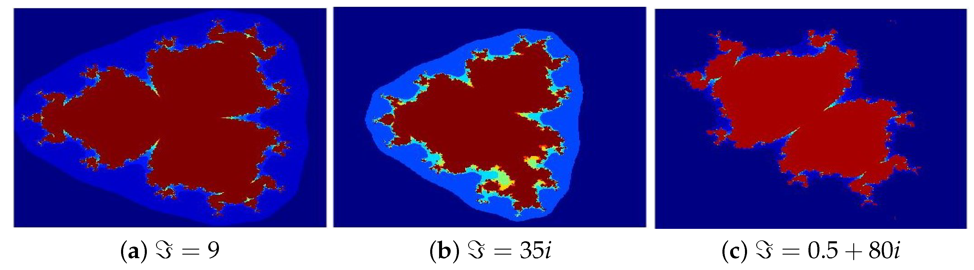
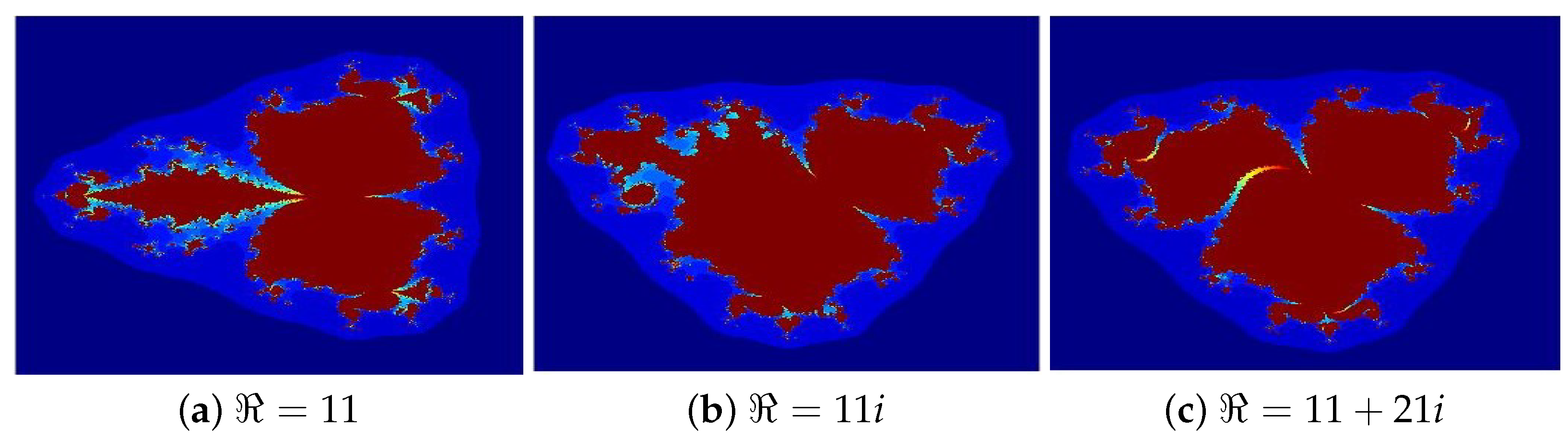
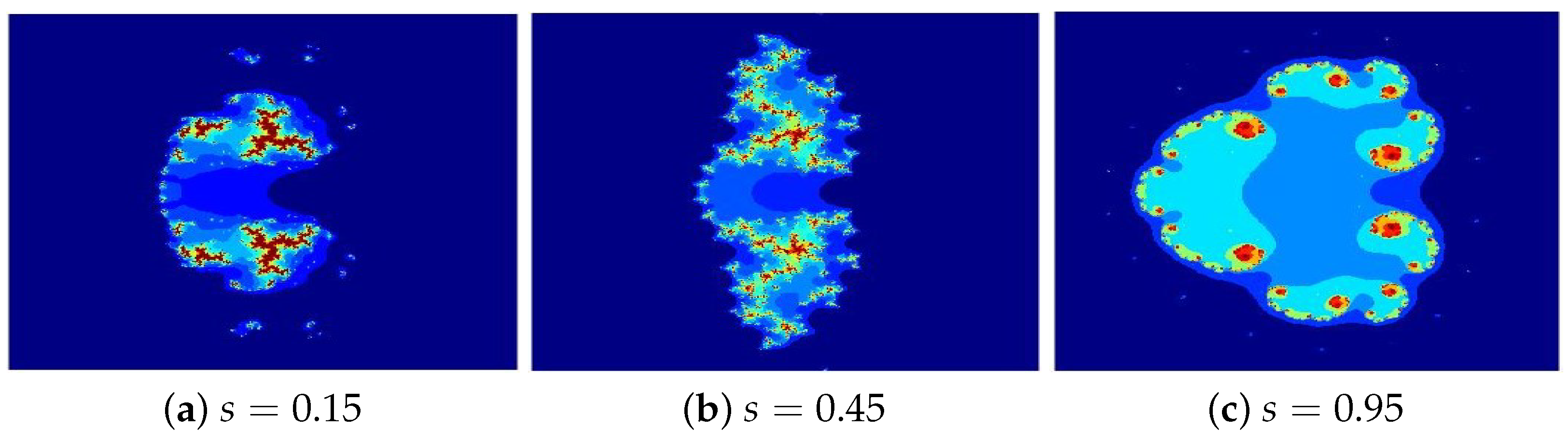
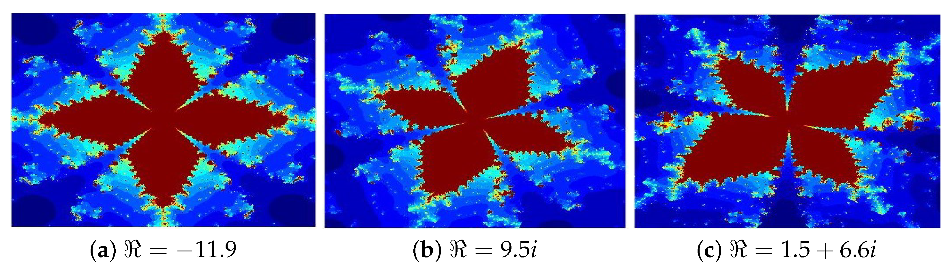
This section presents graphical representations of the Mandelbrot and Julia sets generated using the Jungck–Noor iterative method with s-convexity (see Equation (2)), for different input parameters and exponents $n.$ The visualizations were created through the escape time algorithm, applying the escape criteria derived in Section 3, and were computationally implemented in MATLAB R2019a (Version 9.6.0.1072779, 64-bit). By systematically varying parameter configurations and exponents, we illustrate the diverse fractal structures produced by Algorithms 1 and 2, which detail the iterative and computational procedures for constructing these sets. Specific parameter values and computational settings are provided alongside each figure to ensure reproducibility and clarity in the analysis. Throughout the article, we cover only the behavior of selected fractals for various parameter values, using maximum number of iterations $K=70$, and the color map shown in Figure 1.

4.1. Julia Sets

This subsection presents the Julia sets generated via the Jungck–Noor iterative method with s-convexity for different input values. The execution times for generating these images are also provided in seconds.

The first set of examples explores Julia sets generated using Algorithm 1 with fixed parameters $n=4,\mathsf{\Psi }=0.0005,\mathsf{\Phi }=0.0006,\hslash =0.0007$, and $s=0.55.$

• In Figure 2, the parameters are set to $\Re =100,\omega =-60i$, while ℑ varies across the following cases: (a) 9, (b) 35i, (c) 0.5 + 80i.
• In Figure 3, the parameters are set to $\Im =15,\omega =-60i$, while ℜ varies across the following cases: (a) 11, (b) 11i, (c) 11 + 21i.
• In Figure 4, the parameters are set to $\Im =23,\Re =21$, while $\omega$ varies across the following cases: (a) 35, (b) 55i, (c) 21 + 75i.

The Julia sets depicted in Figure 2, Figure 3 and Figure 4a–c for $n=4$ illustrate the impact of varying individual parameters on fractal morphology while keeping the other two parameters fixed. The subplots (a), (b), and (c) represent purely real, purely imaginary, and complex values, respectively. Variations in the parameters $(\Im ,\Re ,\omega )$ produce significant topological changes; that is, increasing the imaginary components induces contraction while transforming the set’s structure. The resulting patterns display remarkable visual complexity, merging elements reminiscent of traditional Rangoli art with the intricate textures of delicate glass paintings.

Algorithm 1 Geometry of Julia set

Input:  $W\left(z\right)=z^n+\Im z^3+\omega ,T\left(z\right)=\Re z,$ where $\Im ,\Re ,\omega \in \mathbb{C};$ $A\subset \mathbb{C}$-area in which we draw the set; K-maximal number of iterations; colormap $[0..C$-$1]$-color with C colors. Output:  Julia set for area A      for $z_0\in A$ do       $R_1=\frac{2(1+|\Re |)}{s\hslash |\omega ||({\omega }^{n-3}+\Im )|}$       $R_2=\frac{2(1+|\Re |)}{s\mathsf{\Phi }|\omega ||({\omega }^{n-3}+\Im )|}$       $R_3=\frac{2(1+|\Re |)}{s\mathsf{\Psi }|\omega ||({\omega }^{n-3}+\Im )|}$       $R=max\{|\omega |,R_1,R_2,R_3\}$        $p=0$      while $p\le K$ do         $z_{p+1}=\frac{{(1-\mathsf{\Psi })}^{s}T\left(z_p\right)+{\mathsf{\Psi }}^{s}W\left(u_p\right)}{\Re },$       $u_p=\frac{{(1-\mathsf{\Phi })}^{s}T\left(z_p\right)+{\mathsf{\Phi }}^{s}W\left(v_p\right)}{\Re },$       $v_p=\frac{{(1-\hslash )}^{s}T\left(z_p\right)+{\mathsf{\Psi }}^{s}W\left(z_p\right)}{\Re },$   if $|z_{p+1}|\ge R$ then break end if       $p=p+1$       $j=\left[(C-1)\frac{p}{K}\right]$    color $z_0$ with colormap $\left[j\right]$

In the second example, Julia sets are generated using Algorithm 1 with fixed parameters $n=6,\Im =201i,\Re =121i,\omega =55i.$ The images are divided into four groups, each fixing one parameter among $\mathsf{\Psi },\mathsf{\Phi },\hslash ,s$ while varying the others.

• In Figure 5, the parameters are set to $\mathsf{\Phi }=0.06,\hslash =0.09,s=0.75$ while $\mathsf{\Psi }$ varies across the following cases: (a) 0.15, (b) 0.45, (c) 0.85.
• In Figure 6, the parameters are set to $\mathsf{\Psi }=0.18,\hslash =0.07,s=0.75,$ while $\mathsf{\Phi }$ varies across the following cases: (a) 0.25, (b) 0.55, (c) 0.95.
• In Figure 7, the parameters are set to $\mathsf{\Psi }=0.86,\mathsf{\Phi }=0.75,s=0.75$, while ℏ varies across the following cases: (a) 0.005, (b) 0.45, (c) 0.95.
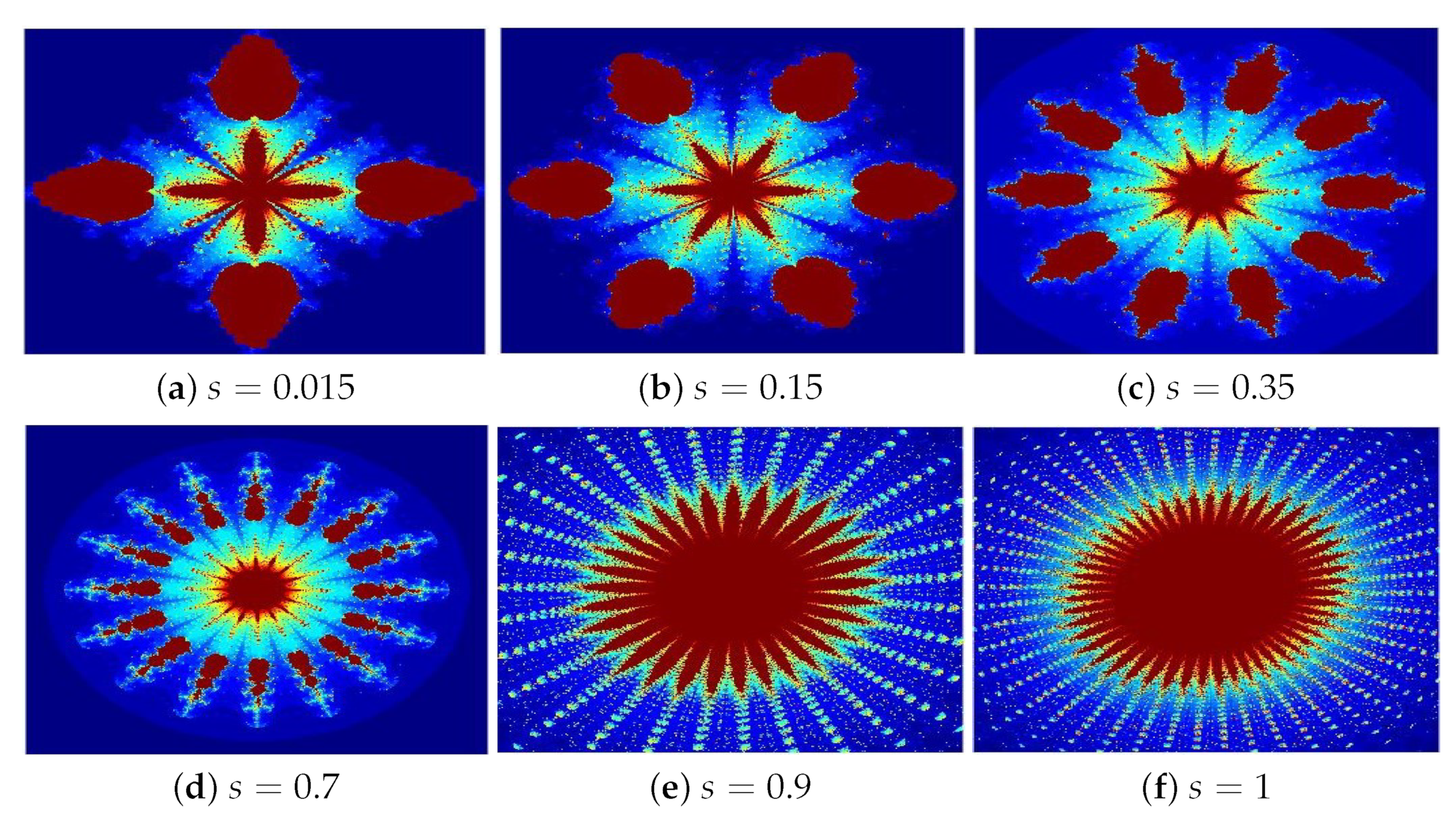
• In Figure 8, the parameters are set to $\mathsf{\Psi }=0.85,\mathsf{\Phi }=0.95,\hslash =0.75$, while s varies across the following cases: (a) 0.15, (b) 0.45, (c) 0.95.

The Julia sets presented in Figure 5, Figure 6, Figure 7 and Figure 8a–c were generated by systematically varying one parameter, either $\mathsf{\Psi }$, $\mathsf{\Phi }$, or ℏ, while holding the other two constant. The results reveal that these parameters play a crucial role in determining the fractal morphology, significantly influencing the shape, size, and color distribution of the sets, particularly along their intricate, leaf-like edges. The resulting patterns exhibit a striking resemblance to traditional Rangoli art, intricate floral designs, and the delicate textures of stained glass, showcasing a mesmerizing interplay of mathematical structure and aesthetic beauty. The patterns evoke Rangoli designs, floral motifs, or delicate glass artwork. The execution times for generating these images are also provided in seconds.

This example generates Julia sets via Algorithm 1, using parameters $\Im =4$, $\Re =100$, $\omega =55i,\mathsf{\Psi }=0.085,\mathsf{\Phi }=0.075,\hslash =0.0095$ and $s=0.88$. By varying n, we examine its impact on the formation and characteristics of the fractal structures.

Figure 9a–f present multiple iterations of a Julia set, with the number of copies following the rule $n-1.$ For instance, when $n=4,$ it produces three copies; when $n=6,$ it yields five copies; and when $n=10,$ it generates nine copies, maintaining this pattern consistently. Each configuration displays $(n-1)$-fold symmetry, creating intricate rosette patterns. These symmetric arrangements consistently retain their visually striking, rosette-like structure.

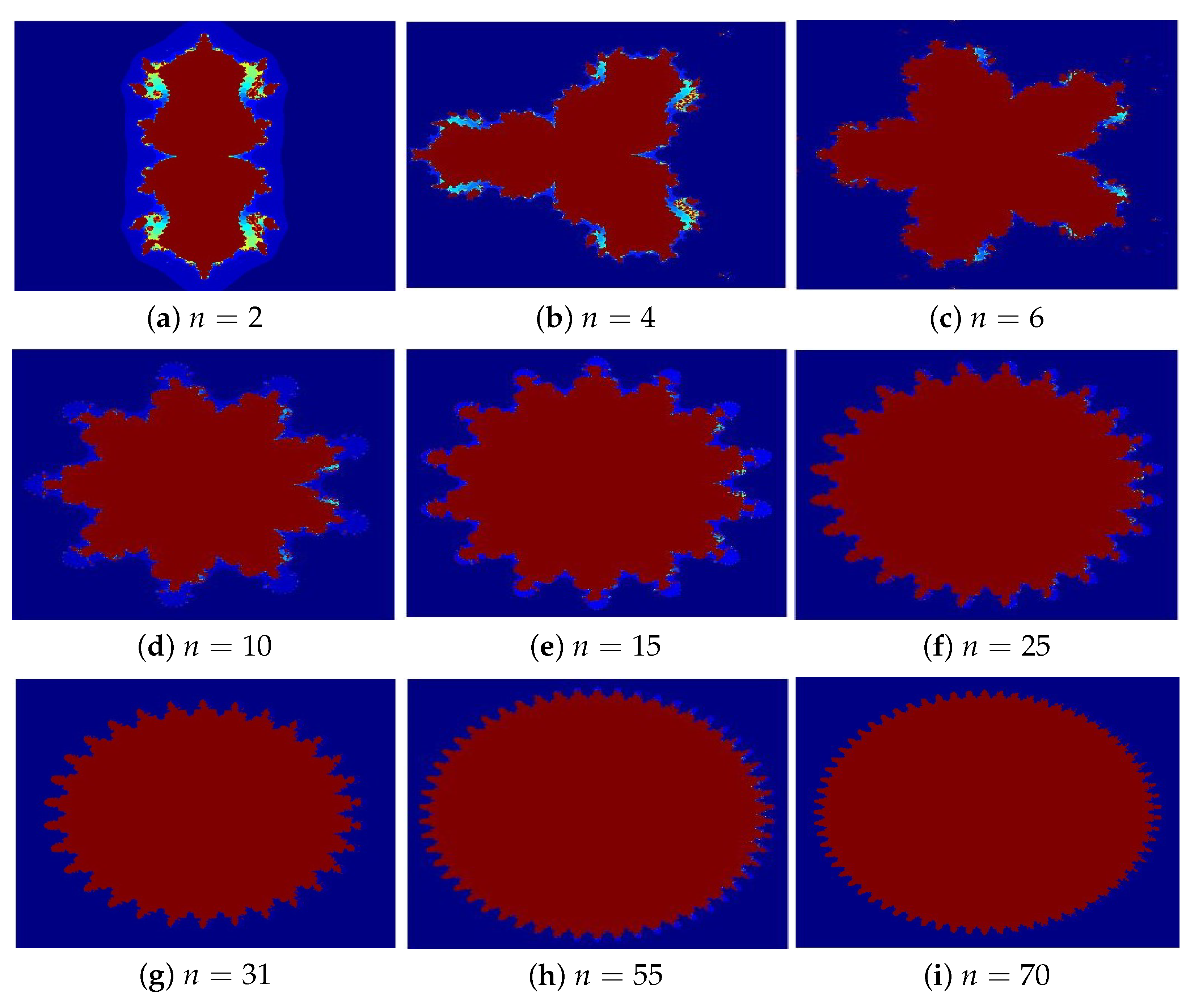
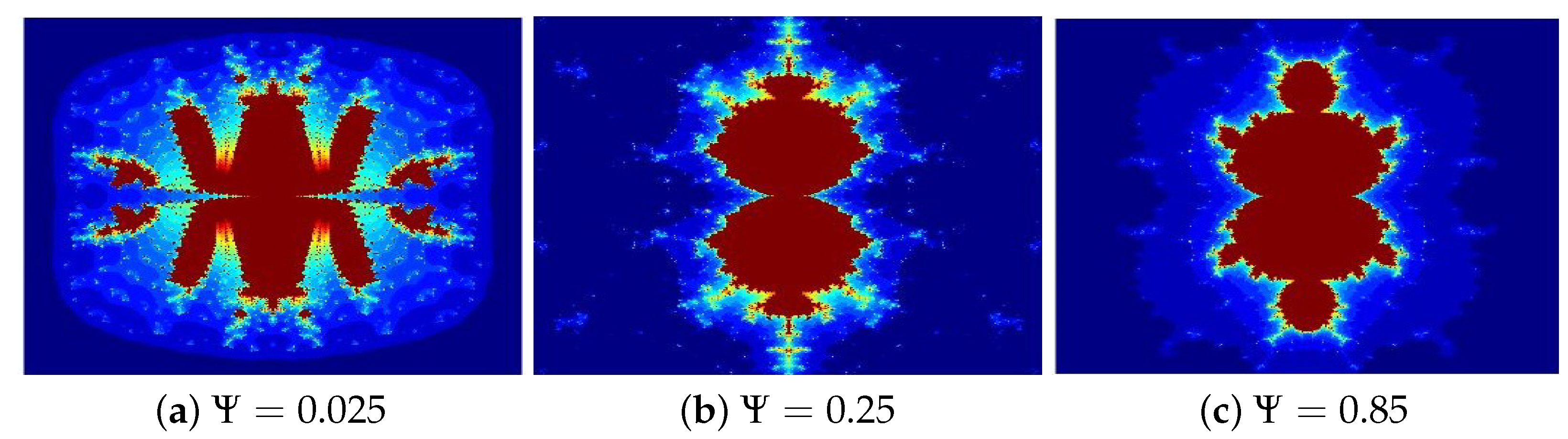
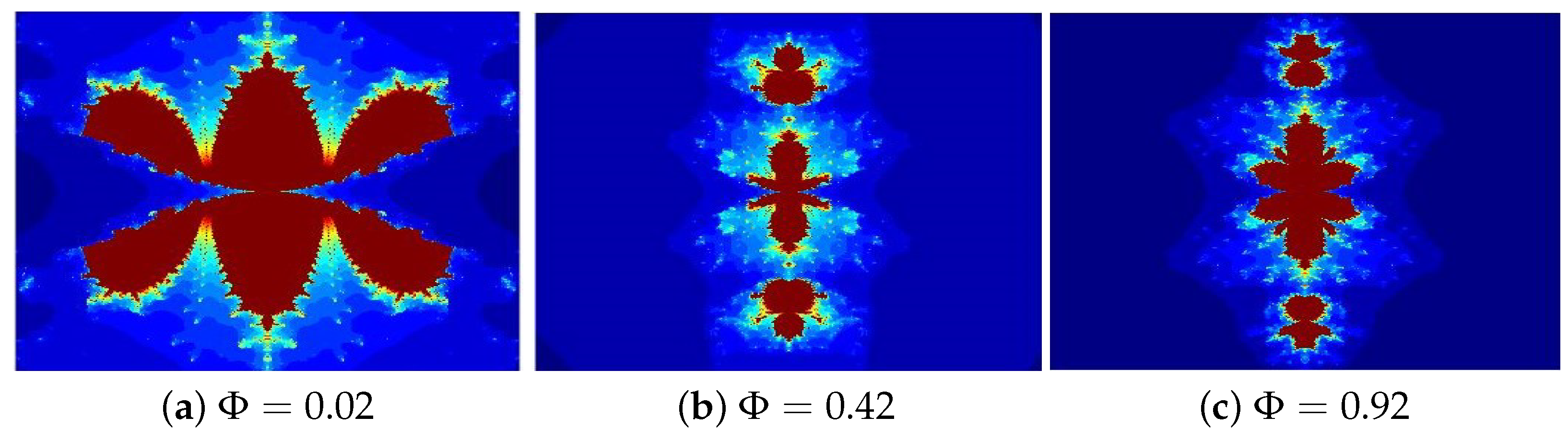
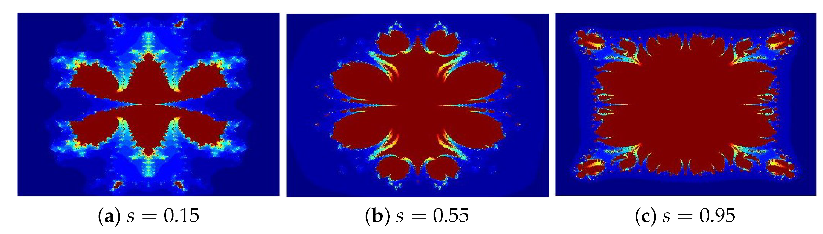
4.2. Mandelbrot Sets

This subsection displays Mandelbrot sets created using Algorithm 2 for the complex function (1) with different parameter values. The execution times for generating these images are also provided in seconds.

The first example explores Mandelbrot sets generated using Algorithm 2, with a maximum iteration limit of $K=70.$ Using parameters $n=5,\mathsf{\Psi }=0.028,\mathsf{\Phi }=0.27,\hslash =0.19$, and $s=0.125,$ the images are divided into two groups, each fixing either parameter ℑ or ℜ while varying the other.

• In Figure 10, the parameters are set to $\Re =-1.9$, while ℑ varies across the following cases: (a) 100, (b) 110i, (c) 100 + 0.1i.
• In Figure 11, the parameters are set to $\Im =0.1i$, while ℜ varies across the following cases: (a) −11.9, (b) 6.5i, (c) 1.5 + 6.6i.

Figure 10 and Figure 11a,b, present Mandelbrot sets with different parameter configurations, as follows: (a) real; (b) imaginary, and (c) complex values for ℑ and ℜ. These parameters significantly influence the fractals’ geometry, coloration, and complexity, with increasing real/imaginary components creating more elaborate structures. The resulting patterns showcase intricate, organic designs resembling Rangoli art, floral motifs, and delicate glasswork.

Algorithm 2 Geometry of the Mandelbrot set

Input:  $W\left(z\right)=z^n+\Im z^3+\omega ,T\left(z\right)=\Re z,$ where $\Im ,\Re ,\omega \in \mathbb{C};$ $A\subset \mathbb{C}$-area in which we draw the set; K-maximal number of iterations; colormap $[0..C$-$1]$-color with C colors. Output:  Mandelbrot set for area A        for $z_0\in A$ do        $R_1=\frac{2(1+|\Re |)}{s\hslash |\omega ||({\omega }^{n-3}+\Im )|}$        $R_2=\frac{2(1+|\Re |)}{s\mathsf{\Phi }|\omega ||({\omega }^{n-3}+\Im )|}$        $R_3=\frac{2(1+|\Re |)}{s\mathsf{\Psi }|\omega ||({\omega }^{n-3}+\Im )|}$        $R=max\{|\omega |,R_1,R_2,R_3\}$        $p=0$        $z_0=0$       while $p\le K$ do         $z_{p+1}=\frac{{(1-\mathsf{\Psi })}^{s}T\left(z_p\right)+{\mathsf{\Psi }}^{s}W\left(u_p\right)}{\Re },$         $u_p=\frac{{(1-\mathsf{\Phi })}^{s}T\left(z_p\right)+{\mathsf{\Phi }}^{s}W\left(v_p\right)}{\Re },$         $v_p=\frac{{(1-\hslash )}^{s}T\left(z_p\right)+{\mathsf{\Psi }}^{s}W\left(z_p\right)}{\Re },$     if $|z_{p+1}|\ge R$ then break end if         $p=p+1$         $j=\left[(C-1)\frac{p}{K}\right]$    color $z_0$ with colormap $\left[j\right]$

This example generates Mandelbrot sets via Algorithm 2, using parameters $n=7$, $\Im =8.8,\Re =1.5.$ The images are organized into four groups, each fixing one parameter $\mathsf{\Psi },\mathsf{\Phi },\hslash ,s$ while varying the others to analyze their effects.

• In Figure 12, parameters $\mathsf{\Phi }=0.0125,\hslash =0.095,s=0.85$ and varying $\mathsf{\Psi }:$ (a) 0.025, (b) 0.25, (c) 0.85.
• In Figure 13, parameters $\mathsf{\Psi }=0.8,\hslash =0.2,s=0.55$ and varying $\mathsf{\Phi }:$ (a) 0.02, (b) 0.42, (c) 0.92.
• In Figure 14, parameters $\mathsf{\Psi }=0.35,\mathsf{\Phi }=0.25,s=0.65$ and varying $\hslash :$ (a) 0.005, (b) 0.35, (c) 0.95.
• In Figure 15, parameters $\mathsf{\Psi }=0.00025,\mathsf{\Phi }=0.015,\hslash =0.055$ and varying $s:$ (a) 0.15, (b) 0.55, (c) 0.95.

The Mandelbrot sets displayed in Figure 12, Figure 13, Figure 14 and Figure 15a–c demonstrate the visual impact of parameter variations while maintaining fixed values for three of the four parameters $\mathsf{\Psi }$, $\mathsf{\Phi },\hslash$, or s. Each subplot systematically explores how individual parameter changes affect the fractal characteristics, with $\mathsf{\Psi }$, $\mathsf{\Phi },\hslash$, or s proving particularly influential in determining the morphological features of the sets. These parameters primarily govern the structural development of leaf-like edge formations while simultaneously controlling overall coloration patterns. The resulting fractals exhibit remarkable aesthetic complexity, bearing strong visual similarities to traditional Rangoli designs, floral arrangements, and delicate stained glass artwork. Notably, the observed geometric patterns reveal a sensitive dependence on parameter values, where minor adjustments produce substantial changes in the fractal’s topological features and visual presentation.

This example generates Mandelbrot sets via Algorithm 2 for functions $T\left(z\right)$ and $W\left(z\right)$, using parameters $\Im =0.001i,\Re =-3i,\mathsf{\Psi }=0.15,\mathsf{\Phi }=0.25,\hslash =0.91$ and $n=7,$ while varying s to analyze its impact on fractal structures.

This example creates Mandelbrot sets using Algorithm 2 for $W\left(z\right)$ and $T\left(z\right)$ with parameters $\Im =0.1i,b=-3.9,\mathsf{\Psi }=0.025,\mathsf{\Phi }=0.45,\hslash =0.01$ and $s=0.71,$ while varying n.

In Figure 16 and Figure 17a–f, we observe multiple copies of the same Mandelbrot set, where the number of copies corresponds to the value of $n.$ For instance, when $n=5,$ there are four copies; when $p=7$, there are six copies; when $p=11$, there are ten copies, and so on. Each pattern exhibits an $(n-1)$-fold radial symmetry, creating an intricate rosette-like design. Despite this, the patterns retain their fascinating rosette-like symmetry. As we vary the values of n, it becomes evident that they greatly impact both the shape and size of the Mandelbrot sets. Additionally, we observe that as the values of n increase, the generated Mandelbrot sets become more complex, with the overall shape of the set undergoing notable changes. The fractals exhibit remarkable, organic designs resembling Rangoli art, floral arrangements, and glass mosaics. The following observations were made:

• The parameters $\Im ,\Re ,c,\mathsf{\Psi },\mathsf{\Phi },\hslash ,s$, and n are critical in determining the structure, scale, and visual properties of the fractals.
• Convergence criteria directly influence image resolution and detail clarity.
• The algorithms generate novel fractal geometries through the complex interplay of $T\left(z\right)$ and $W\left(z\right)$.

5. Conclusions

We developed a novel escape criterion via the Jungck–Noor iteration with s-convexity, enabling the generation of Julia and Mandelbrot sets through Algorithms 1 and 2. Using MATLAB software, we analyzed and discussed the behaviors of various Julia and Mandelbrot sets variations under different parameter values, revealing intriguing non-classical fractals. Our study shows that the size and complexity of these fractals are significantly influenced by parameters $\Im ,\Re ,\omega ,\mathsf{\Psi },\mathsf{\Phi },\hslash ,s$, as well as the exponent $n.$ Even small changes in these parameters can cause significant alterations in the shape, color, and size of the fractals. In future work, we plan to extend this study by generating Julia and Mandelbrot sets through modifications in c, replacing c with $log{c}^t$ in the proposed function. We also aim to incorporate additional metrics, such as generation time and ANI, into these analyses. Furthermore, the findings of this study have practical applications in the textile industry, particularly in the design and printing of patterns.

References

1. Julia, G. Memoire sur l’iteration des fonctions rationnelles. J. Math. Pures Appl. 1918, 8, 47–245. [Google Scholar]
2. Fatou, P. Sur lesequations fonctionnelles. Bull. Soc. Math. Fr. 1919, 47, 161–271. [Google Scholar] [CrossRef]
3. Mandelbrot, B.B. The Fractal Geometry of Nature; Freeman: San Francisco, CA, USA, 1982. [Google Scholar]
4. Kang, S.M.; Rafiq, A.; Latif, A.; Shahid, A.A.; Kwun, Y.C. Tricorns and Multicorns of S-iteration scheme. J. Funct. Spaces 2015, 2015, 417167. [Google Scholar]
5. Kumari, S.; Kumari, M.; Chugh, R. Dynamics of superior fractals via Jungck-SP orbit with s-convexity. An. Univ. Craiova Math. Comput. Sci. Ser. 2019, 46, 344–365. [Google Scholar]
6. Kwun, Y.C.; Tanveer, M.; Nazeer, W.; Gdawiec, K.; Kang, S.M. Mandelbrot and Julia sets via Jungck-CR iteration with s-convexity. IEEE Access 2019, 7, 12167–12176. [Google Scholar] [CrossRef]
7. Nazeer, W.; Kang, S.; Tanveer, M.; Shahid, A. Fixed point results in the generation of Julia and Mandelbrot sets. J. Inequal. Appl. 2015, 2015, 298. [Google Scholar] [CrossRef]
8. Shahid, N.A.; Nazeer, W.; Gdawiec, K. The Picard-Mann iteration with s-convexity in the generation of Mandelbrot and Julia sets. Monatsh. Math. 2021, 195, 565–584. [Google Scholar] [CrossRef]
9. Ahmad, I.; Sajid, M.; Ahmad, R. Julia sets of transcendental functions via a viscosity approximation-type iterative method with s-convexity. Stat. Optim. Inf. Comput. 2024, 12, 1553–1572. [Google Scholar] [CrossRef]
10. Jolaoso, L.; Khan, S.; Aremu, K. Dynamics of RK iteration and basic family of iterations for polynomiography. Mathematics 2022, 10, 3324. [Google Scholar] [CrossRef]
11. Kang, S.; Nazeer, W.; Tanveer, M.; Shahid, A. New fixed point results for fractal generation in Jungck Noor orbit with s-convexity. J. Funct. Spaces 2015, 2015, 963016. [Google Scholar] [CrossRef]
12. Phuengrattana, W.; Suantai, S. On the rate of convergence of Mann, Ishikawa, Noor and SP-iterations for continuous functions on an arbitrary interval. J. Comput. Appl. Math. 2011, 235, 3006–3014. [Google Scholar] [CrossRef]
13. Tanveer, M.; Nazeer, W.; Gdawiec, K. New escape criteria for complex fractals generation in Jungck-CR orbit. Indian J. Pure Appl. Math. 2020, 51, 1285–1303. [Google Scholar] [CrossRef]
14. Zhang, H.X.; Tanveer, M.; Li, Y.X.; Peng, Q.X.; Shah, N.A. Fixed point results of an implicit iterative scheme for fractal generations. AIMS Math. 2022, 6, 13170–13186. [Google Scholar] [CrossRef]
15. Gdawiec, K.; Kotarski, W.; Lisowska, A. On the Robust Newton’s method with the Mann iteration and the artistic patterns from its dynamics. Nonlinear Dynam. 2021, 104, 297–331. [Google Scholar] [CrossRef]
16. Muthukumar, P.; Balasubramaniam, P. Feedback synchronization of the fractional order reverse butterfly-shaped chaotic system and its application to digital cryptography. Nonlinear Dyn. 2013, 74, 1169–1181. [Google Scholar] [CrossRef]
17. Nakamura, K. Iterated inversion system: An algorithm for efficiently visualizing Kleinian groups and extending the possibilities of fractal art. J. Math. Arts 2021, 15, 106–136. [Google Scholar] [CrossRef]
18. Usurelu, G.I.; Bejenaru, A.; Postolache, M. Newton-like methods and polynomiographic visualization of modified Thakur processes. Int. J. Comput. Math. 2021, 98, 1049–1068. [Google Scholar] [CrossRef]
19. Pinheiro, M. s-convexity, foundations for analysis. Differ. Geom. Dyn. Syst. 2008, 10, 257–262. [Google Scholar]
Figure 1. Colormap used in the examples with the Julia and Mandelbrot sets.
Symmetry 17 01028 g001
Figure 2. Julia sets generated via Algorithm 1 with varying . Image execution times are as follows: (a) 1.24 s, (b) 1.45 s, and (c) 1.73 s.
Symmetry 17 01028 g002
Figure 3. Julia sets generated via Algorithm 1 with varying . Image execution times are as follows: (a) 1.34 s, (b) 1.55 s, and (c) 1.83 s.
Symmetry 17 01028 g003
Figure 4. Julia sets generated via Algorithm 1 with varying ω . Image execution times are as follows: (a) 1.38 s, (b) 1.49 s, and (c) 1.63 s.
Symmetry 17 01028 g004
Figure 5. Julia sets generated via Algorithm 1 with varying Ψ . Image execution times are as follows: (a) 1.64 s, (b) 1.85 s, and (c) 2.03 s.
Symmetry 17 01028 g005
Figure 6. Julia sets generated via Algorithm 1 with varying Φ . Image execution times are as follows: (a) 1.54 s, (b) 1.79 s, and (c) 1.98 s.
Symmetry 17 01028 g006
Figure 7. Julia sets generated via Algorithm 1 with varying . Image execution times are as follows: (a) 1.44 s, (b) 1.65 s, and (c) 1.88 s.
Symmetry 17 01028 g007
Figure 8. Julia sets generated via Algorithm 1 with varying s . Image execution times are as follows: (a) 1.54 s, (b) 1.78 s, and (c) 1.93 s.
Symmetry 17 01028 g008
Figure 9. Julia sets generated via Algorithm 1 for different values of n . Image execution times are as follows: (a) 1.64 s, (b) 1.76 s, (c) 1.89 s (d) 2.04 s, (e) 2.15 s, (f) 2.33, (g) 2.44 s, (h) 2.51 s, and (i) 2.63.
Symmetry 17 01028 g009
Figure 10. Mandelbrot sets generated via Algorithm 2 with varying . Image execution times are as follows: (a) 1.14 s, (b) 1.29 s, and (c) 1.43.
Symmetry 17 01028 g010
Figure 11. Mandelbrot sets generated via Algorithm 2 with varying . Image execution times are as follows: (a) 1.44 s, (b) 1.69 s, and (c) 1.96.
Symmetry 17 01028 g011
Figure 12. Julia sets generated via Algorithm 2 with varying Ψ . Image execution times are as follows: (a) 1.64 s, (b) 1.94 s, and (c) 2.23.
Symmetry 17 01028 g012
Figure 13. Julia sets generated via Algorithm 2 with varying Φ . Image execution times are as follows: (a) 1.48 s, (b) 1.88 s, and (c) 2.13.
Symmetry 17 01028 g013
Figure 14. Julia sets generated via Algorithm 2 with varying . Image execution times are as follows: (a) 1.72 s, (b) 1.96 s, and (c) 2.33.
Symmetry 17 01028 g014
Figure 15. Julia sets generated via Algorithm 2 with varying s . Image execution times are as follows: (a) 1.54 s, (b) 1.67 s, and (c) 1.86.
Symmetry 17 01028 g015
Figure 16. Mandelbrot sets generated via Algorithm 2 for different values of s . Image execution times are as follows: Image execution times are as follows: (a) 1.31 s, (b) 1.52 s, (c) 1.43, (d) 1.74 s, (e) 1.98 s, and (f) 2.16.
Symmetry 17 01028 g016
Figure 17. Mandelbrot sets generated via Algorithm 2 for different values of n . Image execution times are as follows: (a) 1.48 s, (b) 1.63 s, (c) 1.93, (d) 2.32 s, (e) 2.46 s, and (f) 2.64.
Symmetry 17 01028 g017
Disclaimer/Publisher’s Note: The statements, opinions and data contained in all publications are solely those of the individual author(s) and contributor(s) and not of MDPI and/or the editor(s). MDPI and/or the editor(s) disclaim responsibility for any injury to people or property resulting from any ideas, methods, instructions or products referred to in the content.