Vehicle Motion State Recognition Method Based on Hidden Markov Model and Support Vector Machine

Abstract

With the development of intelligent transportation, vehicle motion state recognition has become a crucial method for enhancing the reliability of vehicle navigation and ensuring driving safety. Currently, machine learning is the main approach for recognizing vehicle motion states. The symmetry characteristics of sensor data have also been studied to better recognize motion states. However, the existing approaches face challenges during motion state changes due to indeterminate state boundaries, resulting in reduced recognition accuracy. To address this problem, this paper proposes a vehicle motion state recognition method based on the Hidden Markov Model (HMM) and Support Vector Machine (SVM). Firstly, Kalman filtering is applied to denoise the data of inertial sensors. Then, HMM is employed to capture the subtle state transition, enabling the recognition of complex dynamic state changes. Finally, SVM is utilized to classify motion states. The sensor data were collected in various vehicle motion states, including stationary, straight-line driving, lane changing, turning, and then the proposed method is compared with SVM, KNN (K-Nearest Neighbor), DT (Decision Tree), RF (Random Forest), and NB (Naive Bayes). The results of the experiment show that the proposed method improves the recognition accuracy of motion state transitions in the case of boundary ambiguity and is superior to the existing methods.

1. Introduction

A vehicle’s driving trajectory and motion trend is reflected by its motion state. Recognizing vehicle motion states can enhance driving safety and meet the development needs of intelligent transportation and navigation. In urban environments, the vehicle’s motion state is influenced by many factors, such as topography, road conditions, sensor precision, and so on. Thus, extracting valid motion features from a large amount of sensor data and then accurately identifying the vehicle motion state is the key challenge.

At present, there are two kinds of approaches to recognize vehicle motion states. One kind is to use raw sensor data directly, and the other relies on machine learning. In the first kind of approach, raw sensor data is compared with the predefined threshold to detect motion states. Specifically, Hu et al. proposed using vehicle acceleration and speed data as detection values to identify four motion states: acceleration, deceleration, idling, and uniform speed [1]. Yu et al. used IMU (Inertial Measurement Unit) data to classify vehicle motion states based on zero-velocity and non-holonomic constraint criteria, but this method is vulnerable to environment interference [2]. Zhang et al. proposed a driving behavior recognition method based on the spatial–temporal trajectory. This method realizes the real-time detection of turning and speed variation by directly processing vehicle trajectory data [3]. In [4], a vehicle stop-state detection method based on speed threshold was proposed by Yu et al., but it is sensitive to sensor noise and low-speed jitter. In [5], a method of classifying the motion state based on the time window was proposed by analyzing the transfer mechanism of motion states. Kalman filtering (KF) is one of the most common methods for sensor data fusion. An EKF (Extended Kalman Filtering)-based interactive multiple-model method was developed, employing parallel EKF models with dynamic weight adjustment to cope with sudden motion transitions [6]. In [7], an adaptive KF method was used to filter the inertial sensor data, enabling the recognition of various vehicle motion states and improving the accuracy in complex environments. Martí et al. employed unscented KF to fuse IMU, digital compass, and GPS (Global Positioning System) data [8]. In this method, unscented transformation, which is capable of modeling the nonlinear system, is beneficial to estimate motion states. In [9], a MultiWave filter was developed to replace the fixed sliding window, and statistical features were extracted from different sensors and different axes, successfully achieving the recognition of five steering modes. Ye et al. estimated vehicle motion states using model-derived constraints and a Kalman filter, avoiding complex vehicle models [10].

The above approaches are effective in recognizing distinct motion states, but they typically rely on fixed rules, which limit their ability to cope with complex dynamic changes. Additionally, their sensitivity to noise and irregular motion reduces robustness. Machine learning that recognizes complex patterns through training on large datasets can adapt to dynamic changes. It improves robustness to irregular motion and mitigates the limitations of traditional rule-based methods. As a result, machine learning has been increasingly applied to recognize vehicle motion states. In [11], a cascaded Support Vector Machine (SVM) classifier achieved 93% classification accuracy with hierarchical decision-making. In [12], another hierarchical SVM recognition method based on the finite state machine achieved 95.16% accuracy with relatively low computational cost. Li et al. developed a decision tree-based recognition method that reached 95.2% accuracy in distinguishing three basic motion states: stationary, straight-line driving, and turning [13]. Ding et al. developed a triboelectric electrostatic sensing method integrated with Long Short-Term Memory network (LSTM), converting mechanical energy into electrical signals for pattern recognition [14]. Chen et al. designed a panoramic segmentation neural network for driving context recognition, integrating Kalman filtering for motion state prediction to achieve robust estimation [15]. An enhanced temporal Convolutional Neural Network (CNN) can effectively recognize vehicle motion states but encounters computational limitations inherent in deep learning models [16]. A novel multi-dimensional motion perception network is able to perform drift-resistant estimations of vehicle speed and angular velocity, realizing high-precision motion state recognition while maintaining sensitivity to motion details [17]. Jiang et al. proposed a novel Bayesian network that incorporates a filtering method designed to improve data quality and ensure reliable recognition [18]. Wang et al. proposed a serial feature network that achieves 10-class pattern classification by fusing multi-scale spatiotemporal features [19]. In [20], a temporal CNN provided an efficient time-series analysis of vehicle maneuvering patterns, but it poses significant computational demands for modeling long-range temporal dependencies. The hybrid method of CNN and LSTM was developed for vehicle motion state recognition by synergistically combining CNN’s spatial feature extraction with LSTM’s temporal modeling strength [21]. Subsequent improvements have further optimized this hybrid method, including Savitzky–Golay filtering for data denoising [22], SoftMax probability output for reliable confidence estimation [23], and a dual network architecture for complementary feature learning through parallel processing [24]. Peng et al. converted time-series driving data into grayscale images and used a vision transformer with transfer learning to achieve 95.65% accuracy in lane-change prediction [25]. Chen et al. combined an attention-based LSTM with an interactive multiple model (IMM) algorithm to improve prediction by weighting Gaussian process and Kalman filter models [26].

Artificial intelligence methods, such as SVM, CNN, and LSTM, can achieve good classification accuracy; however, CNN requires a complete image to identify a certain motion state, and this limits its real-time performance, resulting in the inability to identify the changes in the motion state in a timely manner. Training LSTM requires a large amount of data and computing power, while SVM performs well when the amount of data is small. More importantly, these methods all have limitations in modeling complex time dependence, and they are difficult for representing implicit transitions between motion states, which limits their ability to recognize continuous state changes. They also lack robustness to noise and ambiguous motion states, leading to a reduced performance in real-world traffic scenarios. Furthermore, the duration of motion states cannot be modeled. To address these issues, this paper proposes a novel hybrid method, which combines the temporal modeling advantage of the Hidden Markov Model (HMM) with the classification capability of SVM. The main contributions of this paper are as follows:

• HMM is introduced to model the complex time dependence. Temporal features of vehicle motion data are extracted based on a state transition mechanism, and implicit state transitions can be modeled, providing more accurate features for motion state recognition.
• By combining HMM with SVM, the limitations of a traditional single model in modeling time-series data are overcome, and the recognition accuracy of vehicle motion states is improved.
• A Kalman filter is applied to denoise the MEMS IMU data, which is more conducive to extracting features from this data.

The remaining paper is organized as follows. In Section 2, the proposed system architecture is introduced, and the implement details of HMM–SVM are explained. In Section 3, three experiments are conducted, respectively, to validate the denoising ability of Kalman filtering, verify the classification performance of HMM–SVM, and present the recognition results of different motion states. Finally, a discussion and some conclusions are provided in Section 4.

2. A Vehicle Motion State Recognition Method Based on HMM–SVM

2.1. System Architecture

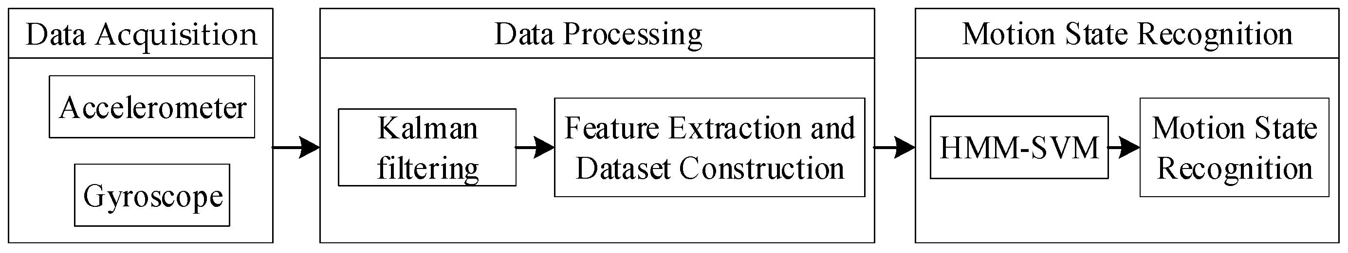
In Figure 1, the proposed system architecture consists of three components: data acquisition, data processing, and motion state recognition. Firstly, triaxial acceleration data and triaxial angular velocity data are collected from MEMS (Micro-Electro-Mechanical Systems). Next, KF is applied to smooth the noise of MEMS data, and multiple features are extracted to build a dataset capable of recognizing different motion states. At last, the HMM–SVM model is trained and used to recognize the vehicle’s motion state.

2.2. Kalman Filter-Based Sensor Data Denoising

KF is a linear estimation algorithm based on minimum mean square error criterion. It recursively predicts and corrects the system state to obtain the optimal estimation. In this paper, the state vector is composed of triaxial acceleration (${\mathit{g}}_{\mathit{k}}$), triaxial angular velocity (${\mathit{\omega }}_{\mathit{k}}$), and angle (${\mathit{\theta }}_{\mathit{k}}$). Therefore, it is represented as follows:

$${\mathit{x}}_{\mathit{k}}={\left[{\mathit{g}}_k,{\mathit{\theta }}_k,{\mathit{\omega }}_k\right]}^T$$

(1)

where ${\mathit{x}}_{\mathit{k}}$ denotes the system state vector.

KF uses both a state equation and measurement equation to estimate the system state. State equation describes the state transition over time, and a linear equation is usually used to predict the system state at the next moment. It is shown as follows:

$${\mathit{x}}_{\mathit{k}}=\mathit{F}{\mathit{x}}_{\mathit{k}-\mathbf{1}}+{\mathit{w}}_{\mathit{k}}$$

(2)

where $\mathit{F}$ represents the state transition matrix, and ${\mathit{w}}_{\mathit{k}}$ represents the process noise vector.

The matrix $\mathit{F}$ is constructed based on the state transition relationship among the members of ${\mathit{x}}_{\mathit{k}}$. Given the time interval ${∆}_t$ between two consecutive states, $\mathit{F}$ is defined as follows:

$$\mathit{F}=\left[\begin{array}{c}1 0 0\\ 0 1 {∆}_t\\ 0 0 1\end{array}\right]$$

(3)

Sensor outputs are taken as the measurement ${\mathit{z}}_{\mathit{k}}$, which is composed of triaxial acceleration (${\mathit{g}}_{\mathit{k}}$), triaxial angular velocity (${\mathit{\omega }}_{\mathit{k}}$), and angle (${\mathit{\theta }}_{\mathit{k}}$). Since ${\mathit{z}}_{\mathit{k}}$ is linearly related to ${\mathit{x}}_{\mathit{k}}$, the measurement equation is as follows:

$${\mathit{z}}_{\mathit{k}}=\mathit{H}{\mathit{x}}_{\mathit{k}}+{\mathit{n}}_{\mathit{k}}$$

(4)

$$\mathit{H}=\left[\begin{array}{c}1 0 0\\ 0 1 0\\ 0 0 1\end{array}\right]$$

(5)

where $\mathit{H}$ represents the measurement matrix, and ${\mathit{n}}_{\mathit{k}}$ represents the measurement noise.

2.3. SVM-Based Motion State Classification

SVM is widely used for pattern recognition, with strong generalization ability and strength in processing high-dimensional data. It achieves high accuracy and stability of the model by maximizing the margin between categories, and it is suitable for complex multi-category classification tasks.

In the case of nonlinearly separable problems, a kernel function is used to map the data to a high-dimensional space, where a linearly separable hyperplane is found for classification. The kernel function computes the inner product of data samples in the high-dimensional space without explicitly performing the mapping. Commonly used kernel functions include linear kernel, polynomial kernel, sigmoid kernel, and RBF (Radial Basis Function) kernel. The RBF kernel has a strong nonlinear fitting ability and wide applicability; thus, it is chosen to solve the linear inseparable problems.

SVM separates two categories by searching a hyperplane in the high-dimensional space to seek the minimum classification error. When using SVM for motion state recognition, the motion states can be mapped to the high-dimensional space through the RBF kernel in Equation (6).

$$R\left({\mathit{v}}_i,{\mathit{v}}_j\right)=exp\left(-{\displaystyle \frac{{‖{\mathit{v}}_i-{\mathit{v}}_j‖}^2}{2{\sigma }^2}}\right)$$

(6)

where $R\left({\mathit{v}}_i,{\mathit{v}}_j\right)$ represents the RBF kernel function, in which ${\mathit{v}}_i$ and ${\mathit{v}}_j$ are two input samples; $exp$ represents the exponential function; ${‖{\mathit{v}}_i-{\mathit{v}}_j‖}^2$ is the squared Euclidean distance, which measures the similarity between two samples; $i$ and $j$ represent the sample indices; and $\sigma$ is the width of the RBF kernel.

When converting the hyperplane solution into a decision function for motion state classification, the decision function is designed as follows:

$$f\left(\mathit{v}\right)=sgn\left[\sum _{i=1}^n{a}_i^{*}{y}_{i}K\left(\mathit{v},{\mathit{v}}_i\right)+b^{*}\right]$$

(7)

where $f\left(\mathit{v}\right),$ which represents the decision function, outputs the classification result; $\mathit{v}$ is the feature vector of the new sample to be classified; $sgn$ represents the sign function, outputting $+1$ or $-1$ based on the operand value; $a_i^{*}$ represents the Lagrange multiplier (support vector weight), in which the superscript $\ast$ denotes the optimal solution; $y_i$ represents the true label of the feature vector ${\mathit{v}}_{\mathit{i}}$; $K\left(\mathit{v},{\mathit{v}}_i\right)$ is the kernel function measuring similarity between two feature vectors; $b^{*}$ represents the bias term, computed through the support vectors; and $n$ represents the number of feature vectors.

$a_i^{*}$ and $b^{*}$ are the core parameters of SVM. The former encodes the classification rule through the selection of support vectors, while the latter adjusts the hyperplane’s position via the bias. In [27], $a_i^{*}$ and $b^{*}$ satisfy the following relationship:

$$\underset{{\mathit{a}}^{*}}{max}\left[\sum _{i=1}^n{a}_i-{\displaystyle \frac{1}{2}}\sum _{i,j}{a}_i{a}_j{y}_i{y}_{j}K\left({\mathit{v}}_i,{\mathit{v}}_j\right)\right]$$

(8)

$$s.t. \sum _{i-1}^n{a}_i{y}_i=0, 0\le a_i\le D$$

(9)

$$b^{*}={\displaystyle \frac{1}{\left|SV\right|}}\sum _{sϵSV}\left(y_s-\sum _{i\in SV}{a}_i^{*}{y}_{i}K\left({\mathit{v}}_i,{\mathit{v}}_s\right)\right)$$

(10)

where $\underset{{\mathit{a}}^{*}}{max}$ represents the maximum value when the variable ${\mathit{a}}^{*}$ is the optimal solution, ${\mathit{a}}^{*}=[a_1^{*};a_2^{*};\dots ;a_n^{*}]$; $s.t.$ denotes the constraints; $D$ represents the penalty parameter, which controls the tolerance for classification errors; and $SV=\left\{i\right|0\le a_i,i=\mathrm{1,2},n\},$ which represents the indices set of all support vectors.

2.4. Modeling Temporal Dependency Based on HMM

Although SVM has good classification performance, its modeling ability for temporal dependence is limited, making it difficult to identify hidden dynamic changes. HMM is capable of modeling long-term dependencies in time series and capturing hidden state transitions, thereby improving the performance of dynamic behavior recognition. In view of this, HMM is introduced to compensate for the shortcomings of SVM.

HMM is a statistical model based on Markov chain theory, typically used to describe time-series data with hidden states. In the proposed method, HMM is used to model the dependence between hidden states and time series. The observation model in HMM follows a polynomial distribution. Its model parameters are obtained by applying the Baum–Welch algorithm, and the hidden state sequence is inferred using the Viterbi algorithm, thereby providing data features for SVM.

The Baum–Welch algorithm iteratively updates HMM parameters to maximize the likelihood of the observed sequence. It is implemented based on the forward–backward process, which outputs the probability of each moment and state. State probabilities and state transition probabilities are calculated using re-estimation formulas until convergence is reached. ${\gamma }_t\left(i\right)$ represents the probability of state $i$ at time $t$, and ${\epsilon }_t\left(i,j\right)$ represents the transition probability from the state $i$ to $j$ at time $t$. ${\gamma }_t\left(i\right)$ and ${\epsilon }_t\left(i,j\right)$ are respectively defined as follows [28]:

$${\gamma }_t\left(i\right)={\displaystyle \frac{{\alpha }_t\left(i\right){\beta }_t\left(i\right)}{\sum _{j=1}^N{\alpha }_t\left(j\right){\beta }_t\left(j\right)}}$$

(11)

$${\epsilon }_t\left(i,j\right)={\displaystyle \frac{{\alpha }_t\left(i\right)p_{ij}{h}_j\left(O_{t+1}\right){\beta }_{t+1}\left(j\right)}{\sum _{i=1}^N\sum _{j=1}^N{\alpha }_t\left(i\right)p_{ij}{h}_j\left(O_{t+1}\right){\beta }_{t+1}\left(j\right)}}$$

(12)

where $p_{ij}$ represents the state transition probability of HMM, reflecting the possibility of transition from state $i$ to state $j$; $i$ and $j$ represent the state indices; $h_j\left(O_{t+1}\right)$ is the probability of observing $O_{t+1}$ given the state $j$; ${\alpha }_t\left(i\right)$ represents the probability of observing the current sequence at time $t$, which is computed using the forward method; ${\beta }_t\left(i\right)$ represents the probability of the future observation sequence given the state $i$ at time $t$, and it is recursively computed using the backward method.

$${\alpha }_t\left(i\right)=\left(\sum _{j=1}^N{\alpha }_{t-1}\left(j\right)p_{ji}\right)h_i\left(O_t\right)$$

(13)

$${\beta }_t\left(i\right)=\sum _{j=1}^N{p}_{ij}{h}_j\left(O_{t+1}\right){\beta }_{t+1}\left(j\right)$$

(14)

where ${\alpha }_{t-1}\left(j\right)$ represents the forward probability at the previous moment; $h_i\left(O_t\right)$ represents the probability of observing $O_t$ given that the system is in state $i$; ${\beta }_{t+1}\left(j\right)$ represents the backward probability at time $t+1$ for state $j$; and $N$ represents the number of states.

The expressions for the transition probability $p_{ij}$, the observation probability $h_j,$ and the initial state distribution probability $e_i$ are the following, respectively:

$$p_{ij}={\displaystyle \frac{{\sum }_{t=1}^{T-1}{\epsilon }_t\left(i,j\right)}{\sum _{t=1}^{T-1}{\gamma }_t\left(i\right)}}$$

(15)

$$h_j\left(u_k\right)={\displaystyle \frac{{\sum }_{t=1}^T{\gamma }_t\left(j\right)·\delta \left(O_t,u_k\right)}{\sum _{t=1}^T{\gamma }_t\left(j\right)}}$$

(16)

$$e_i={\gamma }_1\left(i\right)$$

(17)

where $h_j\left(u_k\right)$ represents the probability of observing $u_k$ given that the system is in the state $j$; $\delta (O_t,u_k)$ represents an indicator function, which equals 1 when the observation $O_t$ is equal to $u_k$ and $0$ otherwise; $e_i$ represents the probability that the state is $i$ at the initial time; and $T$ represents the end time.

Once HMM parameters are obtained, the most likely hidden state can be inferred based on the Viterbi algorithm for a given observation sequence. The optimal path probability refers to the joint probability of the path with the highest probability among all possible hidden state sequences, given the observation sequence $O_t$. The maximum path probability at the initial time is the following:

$${\eta }_1\left(i\right)=e_i{h}_i\left(O_1\right)$$

(18)

where ${\eta }_1\left(i\right)$ represents the joint probability of state $i$ at the initial time ($t=1$); $h_i\left(O_1\right)$ represents the probability of observing $O_1$ given the state $i$.

Then, the maximum probability is recursively calculated as follows:

$${\eta }_t\left(j\right)=\underset{1\le i\le N}{max}\left[{\eta }_{t-1}\left(i\right)·p_{ij}\right]·h_j\left(O_t\right)$$

(19)

The optimal predecessor state ${\phi }_t\left(j\right)$ is defined as follows:

$${\phi }_t\left(j\right)=\underset{1\le i\le N}{\mathit{argmax}}\left[{\eta }_{t-1}\left(i\right)·p_{ij}\right]$$

(20)

$${\phi }_1\left(j\right)=0$$

(21)

where ${\phi }_t\left(j\right)$ represents the optimal preceding state $i$ at time $t-1$, given that the system is in the state $j$ at time $t$.

The optimal state at end time is as follows:

$$q_T=\underset{1\le i\le N}{ar\mathit{gmax}}{[\eta }_T\left(i\right)]$$

(22)

The hidden state at each moment is determined by backtracking. The expression is the following:

$$q_t={\phi }_{t+1}\left(q_{t+1}\right), t=T-1,T-2,\dots 1$$

(23)

At last, the final hidden state sequence $Q=\left(q_1,q_2,\dots q_T\right)$ is obtained for SVM classification.

Furthermore, to transform the hidden state sequences produced by HMM into feature vectors suitable for SVM classification, we employed a sliding window-based feature extraction approach. The size of the sliding window is 25 samples, and the window updates 1 sample each time. Statistical features, such as the occurrence probability of each hidden state, the probability of transitions between each pair of states, and the average duration of each hidden state, are extracted. These features were then concatenated to form the final input vector for SVM. This approach effectively captures the temporal dynamics embedded in the hidden state sequences while maintaining computational efficiency.

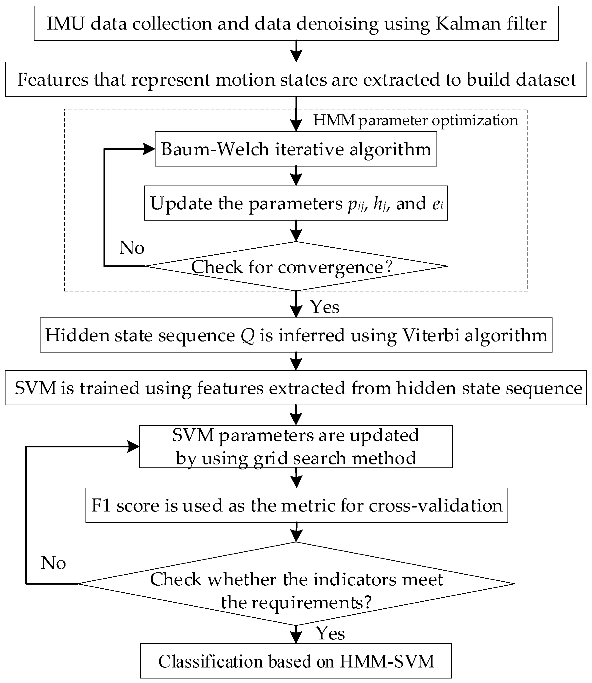
In summary, the whole process of vehicle motion state recognition based on HMM–SVM is shown in Figure 2.

In Figure 2, firstly, real-time motion data collected from the IMU sensor is calibrated, and data noise is smoothed by applying Kalman filtering. Then, distinct features are extracted to construct the training dataset, which is subsequently input into HMM. The parameters (including the state transition probability $p_{ij}$, the observation probability $h_j$, and the state distribution probability $e_i$) of HMM are iteratively updated using the Baum–Welch algorithm until the likelihood function converges to a stable value. The Viterbi algorithm is applied to decode the hidden state sequence $Q$, which reflects the temporal variation of the vehicle’s motion states. Furthermore, high-level features are extracted from the decoded sequence for training SVM, and a grid search is applied to find the optimal parameters of SVM. Five-fold cross-validation was adopted, and the F1 score was used as the evaluation metric. After optimal parameters are obtained, SVM is used as the classifier to recognize motion state.

3. Experiment Results and Analysis

In this experiment, a MEMS IMU WT901SDCL is placed at the front of the vehicle to collect sensor data in various motion states. Meanwhile, data collection covers various road conditions in both urban and rural areas. The parameters of WT901SDCL are shown in

Table 1. The parameters of MEMS.

Parameters	Gyroscope	Accelerometer
Initial bias	400°/h	6000 μgal
In-run bias	10°/h	100 μgal
Scale factor	0.2%	0.2%
Data rate	50 Hz	50 Hz

.

The sensor is first calibrated and then samples the data at a rate of 50 Hz. Noise was removed during the data preprocessing to eliminate irrelevant or erroneous information that could negatively impact the model’s training. Statistical values such as mean, standard deviations, and peak values were generated. The dataset was constructed by using representative statistical values that can reflect motion states. It comprised 50,399 samples, categorized according to different motion states and manually labeled. Moreover, the dataset was partitioned into 24,299 training samples (for model training and parameter optimization) and 26,100 test samples (for validation). Vehicle motion states were classified into four categories: stationary, lane changing, straight driving, and turning, which respectively contained 10,632, 9869, 15,731, and 14,167 samples.

The model’s ability to generalize across various environments was achieved through diverse data collection and the application of data normalization. By collecting data from different road types, weather conditions, and driving behaviors, the model was able to learn the inherent environmental variations and reduce the risk of overfitting. Temporal and spatial diversity further enhanced the model’s adaptability to different temperature and infrastructure types. Normalization ensured consistent sensor data across all conditions. These strategies jointly enhance the robustness of the model, enabling it to perform reliably in various real-world scenarios. To prevent overfitting, model complexity was controlled by regularization and tuning model parameters. Additionally, early stopping was employed by checking the validation results, halting the training process before overfitting occurs.

Three experiments were carried out to validate the proposed method. The first experiment was constructed to show the temporal features of sensor data under different motion states and verify the denoising effect of the Kalman filter. In the second experiment, the performance of five typical machine learning methods in recognizing motion states, as well as the performance of SVM using different kernel functions, was evaluated. In the last experiment, a comparison was made between HMM–SVM and SVM to demonstrate the improvements.

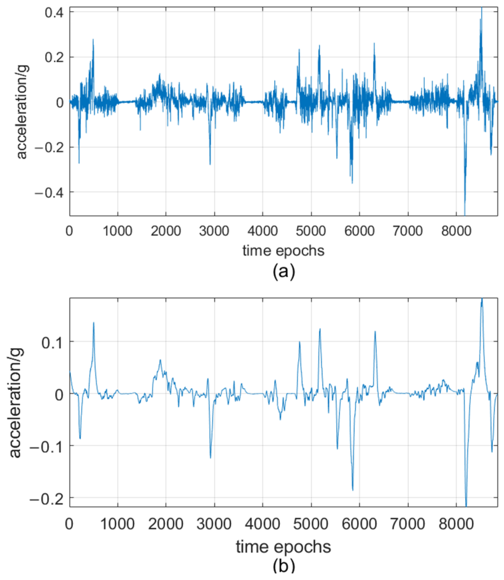
3.1. Sensor Data Denoising and Motion State Illustration

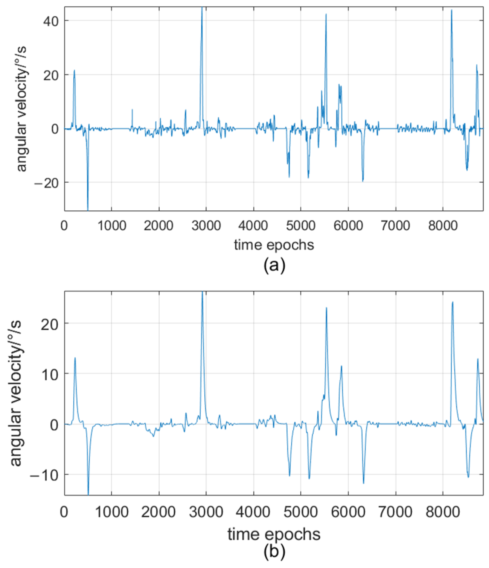
Figure 3 shows the acceleration data before and after applying Kalman filtering. In Figure 3a, the raw data has noticeable noise jitter. In contrast, Figure 3b shows that the filtered data curve becomes smooth and stable, high-frequency noise is suppressed, and the main features of raw data are preserved. Figure 4 illustrates the angular velocity data before and after applying Kalman filtering. Compared with Figure 4a, Figure 4b shows an improvement in smoothness, which can more clearly reflect the true characteristics of angular velocity. The two comparisons prove that Kalman filtering can effectively remove noise from sensor data while retaining the key motion features, which is conducive to the subsequent feature extraction.

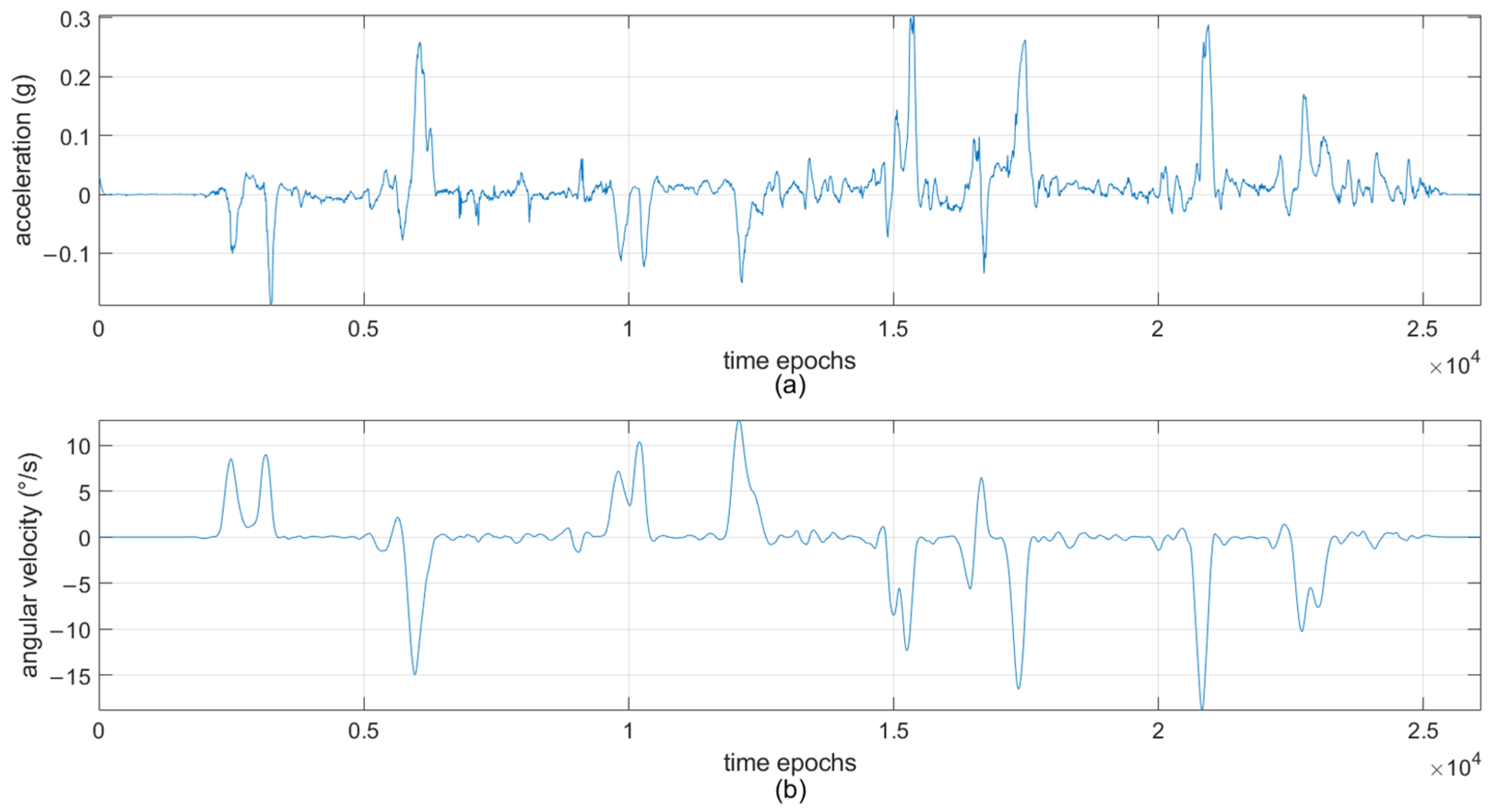
There are four categories of vehicle motion states, and each motion state corresponds to a data feature. In Figure 5, motion states are illustrated through the different features of acceleration data and angular velocity data.

The data points from 650 to 1150 epochs in Figure 5a show the characteristics of the straight driving state, which is represented by slight undulation of the acceleration data. The data points from 1241 to 1600 epochs show the characteristics of the stationary state, and at this time, the acceleration values are close to zero. In Figure 5b, the lane changing state (epochs 120–190) is indicated by a small up-and-down fluctuation of the angular velocity data, which shows the symmetry feature after rotating 180 degrees. This feature is helpful for identifying the dynamic state transition, especially when the boundaries between different states are not clear. The left turning state (epochs 475–593) is characterized by a large fluctuation in the positive direction, while the right turning state (epochs 2305–2440) is characterized by a large fluctuation in the negative direction.

3.2. Performance Comparison of Different Machine Learning Methods

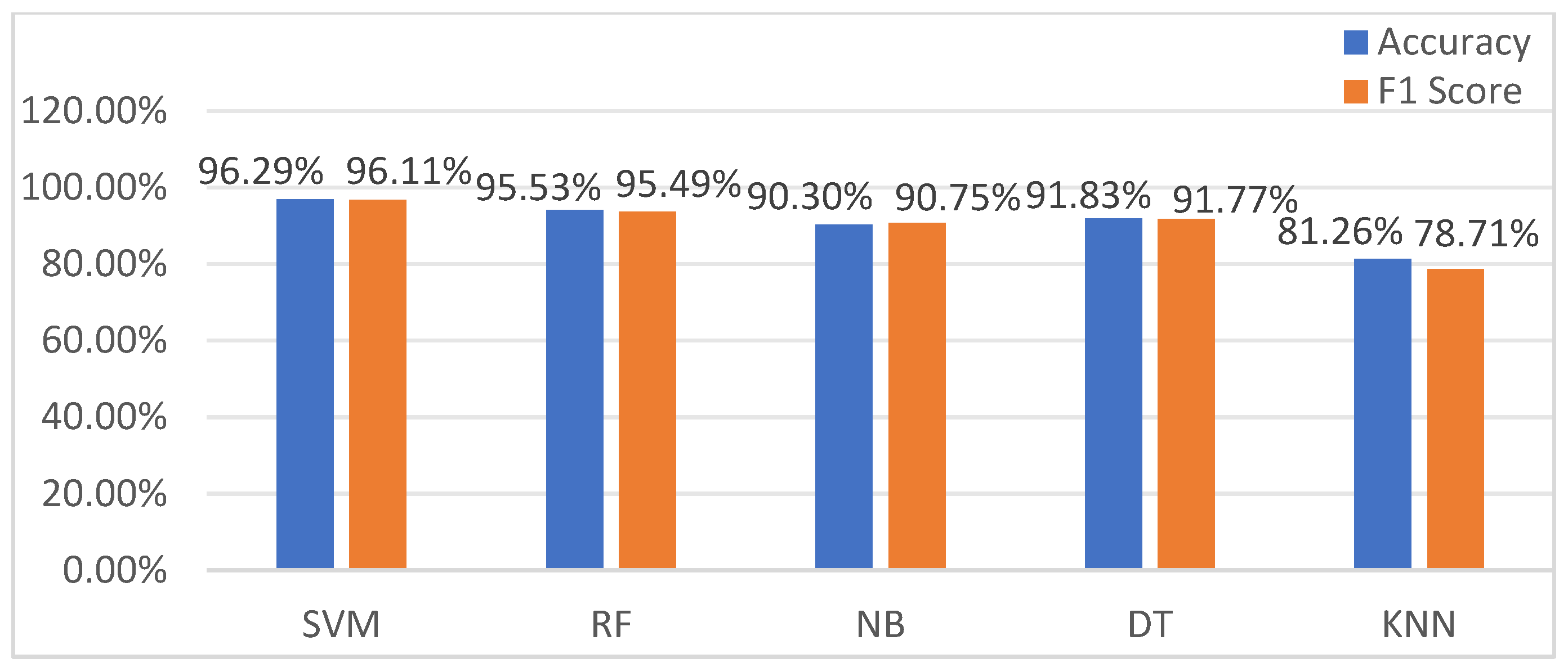
SVM, KNN (K-Nearest Neighbor), DT (Decision Tree), RF (Random Forest), and NB (Naive Bayes) are five common machine learning methods. To ensure fair comparisons, all models were optimized using the grid search method and evaluated through five-fold cross-validation. The parameter configuration was as follows: the regularization parameter of SVM was set to 100 to balance margin maximization against classification error, the kernel coefficient gamma was tuned to 0.1 to control the influence range of the individual training example on the decision boundary. The neighborhood size in KNN was set to 5, which determined the number of samples. Smaller values increased the sensitivity to local patterns, while larger values smoothed the decision boundaries. RF was configured with 100 trees, with a maximum tree depth of 20 to prevent overfitting and a minimum sample size of 2 for internal node splitting. The number of features considered in each segmentation was set as the square root of the total number of features. DT was configured with a maximum tree depth of 10 to balance the model complexity and generalization, a minimum sample size of 2 for node splitting, and a leaf node requirement of 1 to ensure that each terminal node contained sufficient samples. NB adopted a smoothing parameter of 1.0 to avoid the zero probability of unseen features, and the variance stabilization parameter was set to 1 × 10⁻⁹ to ensure the numerical stability during the process of probability calculation.

The experiment results of motion state recognition are presented in Figure 6. KNN has the lowest accuracy and F1 score, while SVM performs best in both assessment indicators, achieving the best classification results.

The performance of SVM depends on the kernel function, which implicitly maps the inseparable low-dimensional data into a higher-dimensional feature space, making the data linearly separable. A comparative test was conducted to evaluate the performance differences of different kernel functions. In

Table 2. Performance comparison of SVM with different kernel functions.

Kernel	Accuracy	Precision	Recall	F1	Runtime
Linear	88.42%	83.73%	88.12%	85.90%	5.8324s
Poly	91.88%	91.47%	90.13%	90.06%	6.4675s
RBF	96.29%	96.17%	96.07%	96.11%	12.3942s
Sigmoid	73.19%	76.00%	72.85%	74.46%	13.0708s

, test results were summarized. The sigmoid kernel performed the worst on all metrics and had the longest runtime. Both the linear kernel and poly kernel had shorter runtimes, but their performance was moderate. The RBF kernel achieved the highest scores in accuracy, precision, recall, and F1 score [29], but it had a long runtime. Overall, the RBF kernel had the best performance, and it was selected as the kernel function of SVM in this paper.

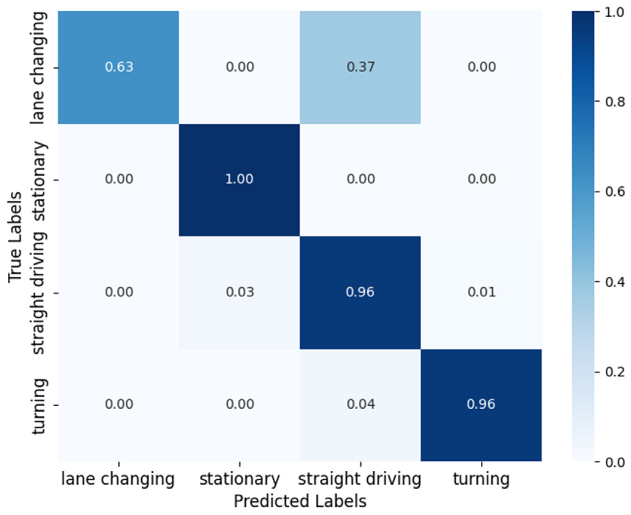
Furthermore, the classification ability of SVM using the RBF kernel is verified, and the confusion matrix of motion states is displayed in Figure 7. In the confusion matrix, rows indicate the true labels, columns indicate the predicted labels, and the value in each cell reflects the classification probability. The “stationary” state achieves high classification accuracy. However, there is confusion in classification between some states. The confusion between “lane changing” and “straight driving” is the most significant, and the probability is 37%. The “straight driving” state is incorrectly classified as “stationary” and “turning”, with a probability of 3% and 1%, respectively. Additionally, there is a slight confusion of 4% between “turning” and “straight driving”. In summary, SVM shows a good discernment for motion states, but further optimization is required to improve accuracy for states with similar characteristics.

3.3. Recognition Results of Motion States

In Section 3.2, it was observed that SVM has difficulty in identifying state transitions between two adjacent states, thereby reducing the classification accuracy. To address this problem, HMM was introduced to combined with SVM to model the adjacent states in this paper.

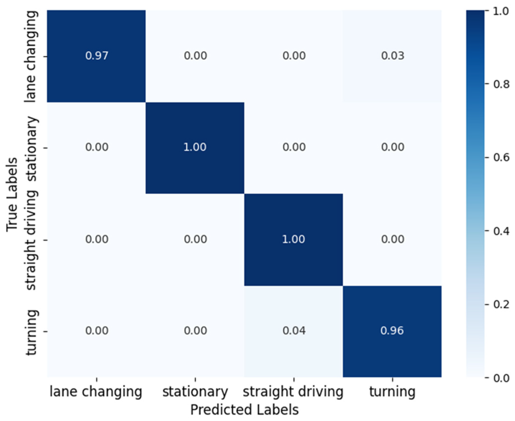
Figure 8 shows the confusion matrix of the proposed method HMM–SVM. As seen in the figure, the motion states “stationary” and “straight driving” can achieve 100% classification accuracy. The “lane changing” state achieves a relatively high accuracy of 97%, with a 3% probability of being incorrectly identified as “turning”, and the “turning” state is wrongly identified as “straight driving” with a probability of 4%. These results indicate that HMM–SVM improves the performance of motion state recognition by integrating the modeling ability of HMM for continuous state transitions.

The performance comparison between SVM and HMM–SVM are presented in

Table 3. The performance of SVM and HMM–SVM.

Algorithm	Accuracy	Precision	Recall	F1
SVM	96.29%	96.17%	96.07%	96.11%
HMM–SVM	98.57%	98.41%	98.36%	97.95%

. The accuracy of HMM–SVM was 98.57%, which is 2.28% higher than that of SVM. The precision was 98.41%, an increase of 2.24%. Recall rate and F1 score increased by 2.29% and 1.84%, respectively.

To confirm the performance improvement of HMM–SVM, we conducted paired t-tests on 10 experiments for each model under the same test conditions. The results show that HMM–SVM outperformed the baseline SVM across all metrics. Specifically, the mean differences in accuracy, precision, recall, and F1 score were 2.28%, 2.24%, 2.29%, and 1.84%, respectively. The corresponding p-values for these metrics were all below 0.004, indicating that the performance improvements achieved by HMM–SVM are statistically significant.

At last, an experiment is constructed to illustrate the visualized results of motion state recognition. Figure 9 displays the filtered angular velocity data and acceleration data in the new test set. Figure 10 presents the recognition results of SVM and HMM–SVM, where the labels are as follows: 0: lane changing; 1: stationary; 2: straight driving; and 3: turning. In comparison with Figure 9, the motion states recognized by both SVM and HMM–SVM between 101 and 5207 epochs are consistent. However, during the lane changing state, between 5450 and 5600 epochs, the state is incorrectly classified as the straight driving state by SVM. Moreover, the turning state is also incorrectly classified by SVM between 9590 and 9680 epochs. On the contrary, HMM–SVM has correct classification and identifies the state transition 36 epochs in advance within 22,100 to 22,490 epochs, which is highly synchronized with the actual changes.

From the above results, it can be concluded that applying SVM achieves accurate recognition in most cases; however, its accuracy decreases during transitions between similar motion states, accompanied by a decline in real-time performance. Thus, SVM has limitations in processing complex motion state transitions. In contrast, HMM–SVM achieves a higher accuracy in motion state recognition and better real-time performance during state transitions. This improvement results from HMM’s ability to model temporal dependency between motion states, enabling the early prediction of state changes and enhancing the recognition performance during dynamic state transitions.

4. Discussion

In this paper, a vehicle motion state recognition method based on HMM–SVM is proposed to address the problem of low recognition accuracy in the presence of sensor noise and indeterminate state boundaries. The raw sensor data is processed by using Kalman filtering, effectively eliminating high-frequency noise and providing high-quality data for subsequent feature extraction. The classification performance of five traditional machine learning methods are compared, and SVM performs the best. However, it has the problem of low accuracy during state transitions. By integrating HMM, long-term dependency in the sequential data can be modeled, compensating for the limitations of SVM. The experiment results show that HMM–SVM is superior to SVM in terms of accuracy, precision, recall rate, and F1 score. The next plan is to further improve the accuracy of identifying small turns and small lane changes. In particular, on bumpy roads, the sensor data contains more interference, making the identification of these two states more difficult and requiring the exploration of new methods.