A Discrete-Time Neurodynamics Scheme for Time-Varying Nonlinear Optimization with Equation Constraints and Application to Acoustic Source Localization

Abstract

Nonlinear optimization with equation constraints has wide applications in intelligent control systems, acoustic signal processing, etc. Thus, effectively tackling the nonlinear optimization problems with equation constraints is of great significance for the advancement of these fields. Current discrete-time neurodynamics predominantly addresses unperturbed optimization scenarios, exhibiting inherent sensitivity to external noise, which limits the practical application of these methods. To address this issue, we propose a discrete-time noise-suppressed neurodynamics (DTNSN) model in this paper. First, the model integrates the static optimization stability of the gradient-based neurodynamics (GND) model with the time-varying tracking capability of the zeroing neurodynamics (ZND) model. Then, an integral feedback term is introduced to suppress external noise disturbances, thereby enhancing the robustness of the model. Additionally, to facilitate implementation on digital hardware, we employ an explicit linear three-step discretization method to obtain the proposed DTNSN model. Finally, the convergence performance, noise suppression capability, and practicality of the model are validated through theoretical analysis, numerical simulations, and acoustic source localization experiments. The model is applicable to the fields of intelligent control systems, acoustic signal processing, and industrial automation, providing new tools for real-time optimization in noisy environments.

1. Introduction

Optimization problems are prevalent in mathematics [1,2], computer science [3,4], and various engineering and technology fields [5,6]. This has generated extensive research interest [7,8]. Among them, nonlinear optimization [9,10,11] is an important subfield. Symmetric and asymmetric phenomena are of great significance in our current research for dynamic optimization problems. Many optimization problems inherently have a symmetric structure; for example, the objective function and constraints may maintain some invariance under variable substitution or parameter transformation. This inherent symmetry can help us simplify the problem solving process and provide a theoretical basis for designing efficient algorithms. For example, when dealing with optimization problems with symmetric constraints, the use of symmetry can reduce the computational complexity and improve the efficiency of the solution. A novel diagonal quasi-Newton algorithm was recently proposed in [9] to address unconstrained nonlinear optimization by adaptively updating the diagonal entries of the approximate Hessian matrix via a specialized rule. However, practical applications such as robotic control [12], power system management [13], and real-time signal processing [14] frequently involve time-varying constraints that evolve over time. For instance, Wu et al. introduced the discrete adaptive zeroing neurodynamics (DAZND) model to solve optimization problems with time-varying equation constraints. They validated its efficacy through robotic arm attitude and position tracking experiments [10]. From the above, it can be seen that in practical applications, the dynamics of the problem and the uncertainty of the environment often introduce asymmetric factors. These factors destroy the original symmetric structure. This asymmetry brings additional challenges to the design of optimization algorithms. Our research is based on a deep understanding of the relationship between symmetry and asymmetry. Our goal is to develop optimization methods that can adapt to dynamic environments and deal with complex constraints, which will help to deal with complex situations in real engineering.

Neurodynamics [15,16,17,18] has emerged as a promising approach for solving such optimization problems due to its parallel processing capabilities and potential for real-time processing. Among various neurodynamics methods, recurrent neurodynamics (RND) is applied in several engineering domains, including optimization [19], robot control [20], and equation solving [21]. Gradient-based neurodynamics (GND), a specialized variant of RND, initially defines an energy function based on a specific paradigm and subsequently approximates the optimal solution using gradient descent [22]. GND exhibits rapid convergence when the gradient is sufficiently large. In a study conducted by Zhang et al. [23], equation-constrained optimization was tackled using the GND approach, confirming the convergence of the model. However, despite advances in technology, GND has an unavoidable hysteresis error in dynamic scenarios. To address these limitations, zeroing neurodynamics (ZND) has been progressively refined and enhanced, emerging as the predominant solution for dynamic problems. The ZND model reformulates optimization problems into error-based functions that force the error to converge to zero. The solution derived from the error function is equivalent to the optimal solution of the original optimization problem [24]. Furthermore, the convergence of the ZND model for solving time-varying nonlinear systems of equations has been validated [25]. Additionally, ZND can be applied to mobile localization [26], manipulator control [27], fuzzy control [28], and joint constraints [29].

Given the prevalence of noise in engineering applications—such as circuit disturbances, real-time plant control challenges [30], and sudden unpredictable perturbations [31]—effective noise suppression capability is critical for the practical utility of models. Although the GND and ZND models are widely employed for solving equation-constrained optimization problems, they exhibit significant residual errors and remain poorly noise resistant [32]. As noted in [33], the model after integrating GND and ZND appears to have poor robustness of its model because it does not pay attention to the presence of external noise. Additionally, in [34], Li et al. used a fourth-order finite difference formulation to discretize a continuous ZND model to obtain the FIFD-K model and the FIFD-U model. These two models are used to solve nonlinear optimization problems containing time-varying equation constraints, but again without considering the interference of external noise. In addition, in [35], Liufu et al. proposed improved noise-resistant neurodynamics to solve nonlinear optimization problems with equation constraints, but the constraint problem is a static constraint problem that does not take into account constraints that change in real time. Therefore, it is crucial to develop a new algorithm that can effectively reduce noise disturbances (e.g., constant noise disturbances, time-varying noise disturbances, random noise disturbances) in a nonlinear optimization problem with time-varying equation constraints.

Therefore, in this paper, a discrete-time noise-suppressed neurodynamics (DTNSN) model is constructed for solving time-varying nonlinear problems with equation constraints. The model combines the strengths of GND and ZND. It uses the gradient information from the GND model. When the gradient is large enough, GND shows rapid convergence. Additionally, the model incorporates the time derivative from the ZND approach to obtain the exact solution. To enhance the model’s robustness and overcome the limitations of GND and ZND, we add an integral feedback term. This improves the model’s accuracy and resilience. In addition, the model is discretized using an explicit linear three-step method [36], facilitating implementation on digital platforms while enhancing both accuracy and flexibility. Figure 1 shows the block diagram of the model of DTNSN. The contributions of this paper are as follows:

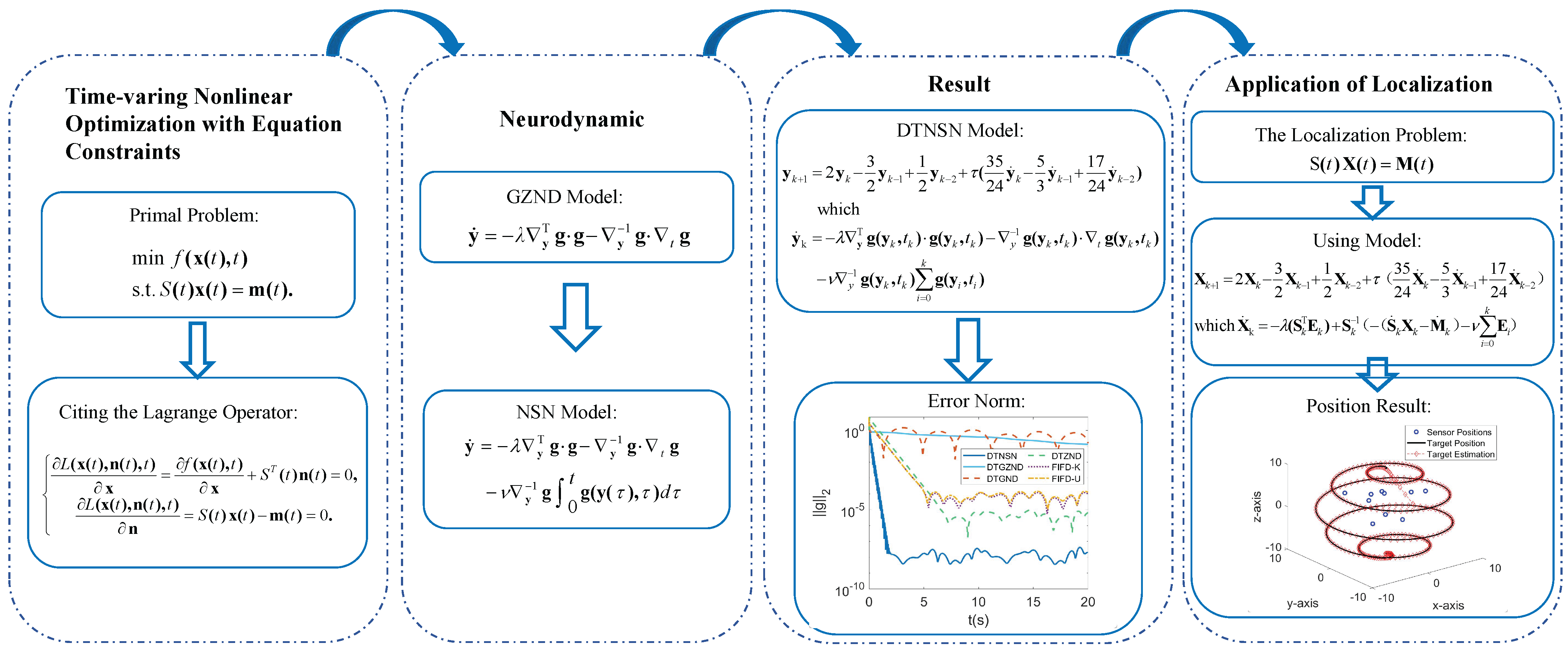
• In this paper, a DTNSN model is constructed as a solution for time-varying nonlinear optimization with equation constraints. The DTNSN model has good convergence performance and noise suppression compared with existing models.
• The DTNSN model uses an explicit linear three-step discretization method and is therefore easier to implement in hardware.
• In numerical simulations, the DTNSN model shows good convergence performance and noise suppression in many types of time-varying nonlinear optimization problems with equation constraints.
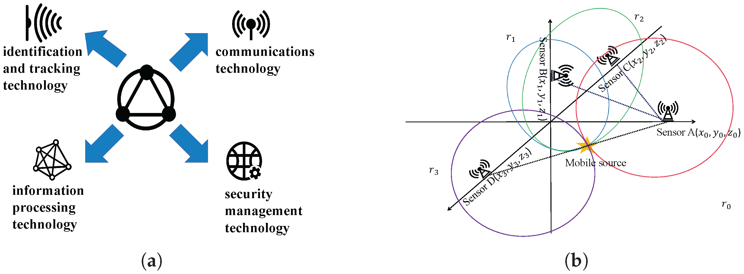
• The DTNSN model is successfully applied to acoustic source localization and proves its utility with better performance than the traditional Kalman filter.

The remainder of this paper comprises four sections. Section 2 focuses on time-varying nonlinear optimization with equation constraints, introduces the construction of the DTNSN, and gives five models for comparison. Section 3 presents theoretical proofs to demonstrate the global stability and robustness of the DTNSN model under noise disturbances. Section 4 demonstrates the convergence, robustness, and practicality of the DTNSN model through its numerical simulation and application in acoustic source localization. Finally, Section 5 summarizes the study and suggests future research directions.

2. Problem Statement and Model Construction

2.1. Problem Statement

A class of time-varying nonlinear optimization with equation constraints is studied in this paper. The problem is denoted as

$$\begin{array}{cc}\hfill & minf\left(\mathbf{x}\right(t),t),\hfill \\ \hfill & \mathrm{s}.\mathrm{t}.S\left(t\right)\mathbf{x}\left(t\right)=\mathbf{m}\left(t\right).\hfill \end{array}$$

(1)

Among them, the objective function $f\left(\mathbf{x}\right(t),t)$ is a second-order integrable nonlinear and convex function at $t>0$, $\mathbf{x}\left(t\right)\in {\mathbb{R}}^p$ is a decision variable that is time-varying, t is a non-negative time variable, and the formula $S\left(t\right)\mathbf{x}\left(t\right)=\mathbf{m}\left(t\right)$ is a time-varying linear constraint where $S\left(t\right)\in {\mathbb{R}}^{q\times p}$.

2.2. Continuous Time Modeling

To solve this problem (1), the Lagrangian operator is introduced and the Lagrangian function is

$$L(\mathbf{x}\left(t\right),\mathbf{n}\left(t\right),t)=f(\mathbf{x}\left(t\right),t)+{\mathbf{n}}^{\mathrm{T}}\left(t\right)(S\left(t\right)\mathbf{x}\left(t\right)-\mathbf{m}\left(t\right)),$$

(2)

where $\mathbf{n}\left(t\right)={\left[n_1\left(t\right),\cdots ,n_q\left(t\right)\right]}^{\mathrm{T}}\in {\mathbb{R}}^q$ is the Lagrange multiplier vector and the superscript ^T denotes the vector or matrix transposition. According to the assumptions of the Lagrangian method, the problem under consideration can be solved by introducing the following system of equations:

$$\left\{\begin{array}{c}{\displaystyle \frac{\partial L\left(\mathbf{x}\right(t),\mathbf{n}(t),t)}{\partial \mathbf{x}}}={\displaystyle \frac{\partial f\left(\mathbf{x}\right(t),t)}{\partial \mathbf{x}}}+S^{\mathrm{T}}\left(t\right)\mathbf{n}\left(t\right)=\mathbf{0},\hfill \\ {\displaystyle \frac{\partial L\left(\mathbf{x}\right(t),\mathbf{n}(t),t)}{\partial \mathbf{n}}}=S\left(t\right)\mathbf{x}\left(t\right)-\mathbf{m}\left(t\right)=\mathbf{0}.\hfill \end{array}\right.$$

(3)

The above system of equations can be converted into another form by the following changes:

$$\begin{array}{cc}\hfill \mathbf{g}\left(\mathbf{y}\right(t),t)=& \left[\begin{array}{c}{\displaystyle \frac{\partial f\left(\mathbf{x}\right(t),t)}{\partial \mathbf{x}}}+S^{\mathrm{T}}\left(t\right)\mathbf{n}\left(t\right)\\ S\left(t\right)\mathbf{x}\left(t\right)-\mathbf{m}\left(t\right)\end{array}\right]\hfill \\ \hfill =& \left[\begin{array}{c}{g}_1(\mathbf{y}\left(t\right),t)\\ ⋮\\ g_p(\mathbf{y}\left(t\right),t)\\ g_{p+1}(\mathbf{y}\left(t\right),t)\\ ⋮\\ g_{p+q}(\mathbf{y}\left(t\right),t)\end{array}\right]=0\in {\mathbb{R}}^{p+q},\hfill \end{array}$$

(4)

which $\mathbf{y}\left(t\right)={\left[{\mathbf{x}}^{\mathrm{T}}\left(t\right),{\mathbf{n}}^{\mathrm{T}}\left(t\right)\right]}^{\mathrm{T}}=[y_1\left(t\right),\cdots ,y_{p+1}\left(t\right),\cdots ,{\left.y_{p+q}\left(t\right)\right]}^{\mathrm{T}}\in {\mathbb{R}}^{p+q}$.

By introducing the ZND design formula, we define

$$\dot{\mathbf{g}}(\mathbf{y}\left(t\right),t)=-\lambda \mathbf{g}(\mathbf{y}\left(t\right),t),$$

(5)

where $\dot{\mathbf{g}}(\mathbf{y}\left(t\right),t)$ is the time derivative of $\mathbf{g}\left(\mathbf{y}\right(t),t)$ and the design parameter $\lambda >0$. We set the time derivative of $\mathbf{g}$ as

$$\begin{array}{c}\hfill \dot{\mathbf{g}}(\mathbf{y}\left(t\right),t)={\displaystyle \frac{\partial \mathbf{g}\left(\mathbf{y}\right(t),t)}{\partial {\mathbf{y}}^{\mathrm{T}}}}\dot{\mathbf{y}}\left(t\right)+{\displaystyle \frac{\partial \mathbf{g}\left(\mathbf{y}\right(t),t)}{\partial t}}={\nabla }_{\mathbf{y}}\mathbf{g}·\dot{\mathbf{y}}+{\nabla }_t\mathbf{g},\end{array}$$

(6)

where $\dot{\mathbf{y}}\left(t\right)$ denotes the time derivative of $\mathbf{y}\left(t\right)$, ${\nabla }_{\mathbf{y}}\mathbf{g}$ denotes the partial derivative of $\mathbf{g}$ with respect to $\mathbf{y}$, ${\nabla }_t\mathbf{g}$ denotes the partial derivative of $\mathbf{g}$ with respect to t, and $\mathbf{g}$ is equivalent to $\mathbf{g}\left(\mathbf{y}\right(t),t)$. The ZND model can be derived as follows:

$$\dot{\mathbf{y}}=-\lambda {\nabla }_{\mathbf{y}}^{-1}\mathbf{g}·\mathbf{g}-{\nabla }_{\mathbf{y}}^{-1}\mathbf{g}·{\nabla }_t\mathbf{g},$$

(7)

where the superscript ⁻¹ is the pseudo-inverse of a matrix or dimension vector and $\lambda \in {\mathbb{R}}^{+}$. Given the efficacy of gradient descent in addressing optimization problems, the energy function is defined as $\hslash ={\parallel \mathbf{g}\parallel }_2^2/2$. The GND model can be derived as follows:

$$\dot{\mathbf{y}}=-\lambda {\nabla }_{\mathbf{y}}\hslash =-\lambda {\nabla }_{\mathbf{y}}^{\mathrm{T}}\mathbf{g}·\mathbf{g}.$$

(8)

The integration of Equations (7) and (8) results in the GZND model, as follows:

$$\dot{\mathbf{y}}=-\lambda {\nabla }_{\mathbf{y}}^{\mathrm{T}}\mathbf{g}·\mathbf{g}-{\nabla }_{\mathbf{y}}^{-1}\mathbf{g}·{\nabla }_t\mathbf{g}.$$

(9)

To enhance the robustness of the model and reduce errors, we introduce an integral feedback term given by $\dot{\mathbf{g}}(\mathbf{y}\left(t\right),t)=-\lambda \mathbf{g}(\mathbf{y}\left(t\right),t)-\nu {\int }_0^t\mathbf{g}(\mathbf{y}\left(\tau \right),\tau )\mathrm{d}\tau$. This term can be incorporated into the noise-suppressed neurodynamics (NSN) model as follows:

$$\dot{\mathbf{y}}=-\lambda {\nabla }_{\mathbf{y}}^{\mathrm{T}}\mathbf{g}·\mathbf{g}-{\nabla }_{\mathbf{y}}^{-1}\mathbf{g}·{\nabla }_t\mathbf{g}-\nu {\nabla }_{\mathbf{y}}^{-1}\mathbf{g}{\int }_0^t\mathbf{g}(\mathbf{y}\left(\tau \right),\tau )\mathrm{d}\tau ,$$

(10)

where $\nu \in {\mathbb{R}}^{+}$. In order to conduct further research on the robustness of the NSN model (10) in the presence of unknown noisy disturbances, the following improved model is proposed:

$$\begin{array}{c}\hfill \dot{\mathbf{y}}=-\lambda {\nabla }_{\mathbf{y}}^{\mathrm{T}}\mathbf{g}·\mathbf{g}-{\nabla }_{\mathbf{y}}^{-1}\mathbf{g}·{\nabla }_t\mathbf{g}-\nu {\nabla }_{\mathbf{y}}^{-1}\mathbf{g}{\int }_0^t\mathbf{g}(\mathbf{y}\left(\tau \right),\tau )\mathrm{d}\tau +{\nabla }_{\mathbf{y}}^{-1}\mathbf{g}·\mathit{\vartheta }\left(t\right),\end{array}$$

(11)

where $\mathit{\vartheta }\left(t\right)$ is the unknown noise.

2.3. DTNSN Model

The objective of this section is to facilitate the implementation of the model on a digital platform. To that end, the corresponding discrete-time model is constructed. First of all, for the acquisition of the discrete-time model, an explicit linear three-step discretization method [36] is given as follows:

$$\begin{array}{c}\hfill {\mathbf{y}}_{k+1}=2{\mathbf{y}}_k-{\displaystyle \frac{3}{2}}{\mathbf{y}}_{k-1}+{\displaystyle \frac{1}{2}}{\mathbf{y}}_{k-2}+\tau \left({\displaystyle \frac{35}{24}}{\dot{\mathbf{y}}}_k-{\displaystyle \frac{5}{3}}{\dot{\mathbf{y}}}_{k-1}+{\displaystyle \frac{17}{24}}{\dot{\mathbf{y}}}_{k-2}\right)+\mathbf{O}\left({\tau }^4\right),\end{array}$$

(12)

where $\tau$ represents the sampling interval and $t_k=k\tau$; the truncation error is $\mathbf{O}\left({\tau }^4\right)$.

Since the use of the explicit linear three-step method requires knowledge of the y-values of the first three steps, when constructing the DTNSN model, the Eulerian discretization is used to discretize (10) to obtain the required preliminary y-value information, and then (10) is discretized by using the explicit linear three-step method, which ultimately results in the DTNSN model. When $k=0,1,2$,

$$\begin{array}{c}\hfill {\mathbf{y}}_{k+1}={\mathbf{y}}_k+\tau {\dot{\mathbf{y}}}_k,\end{array}$$

where

$$\begin{array}{c}\hfill {\displaystyle {\dot{\mathbf{y}}}_k=-\lambda {\nabla }_{\mathbf{y}}^{\mathrm{T}}\mathbf{g}\left({\mathbf{y}}_k,t_k\right)·\mathbf{g}\left({\mathbf{y}}_k,t_k\right)-{\nabla }_{\mathbf{y}}^{-1}\mathbf{g}\left({\mathbf{y}}_k,t_k\right)·{\nabla }_t\mathbf{g}\left({\mathbf{y}}_k,t_k\right)-\nu {\nabla }_{\mathbf{y}}^{-1}\mathbf{g}\left({\mathbf{y}}_k,t_k\right)\sum _{i=0}^{\kappa }\mathbf{g}\left({\mathbf{y}}_i,t_i\right).}\end{array}$$

When $k=3,\cdots ,\varkappa -1$,

$$\begin{array}{c}\hfill {\mathbf{y}}_{k+1}=2{\mathbf{y}}_k-{\displaystyle \frac{3}{2}}{\mathbf{y}}_{k-1}+{\displaystyle \frac{1}{2}}{\mathbf{y}}_{k-2}+\tau \left({\displaystyle \frac{35}{24}}{\dot{\mathbf{y}}}_k-{\displaystyle \frac{5}{3}}{\dot{\mathbf{y}}}_{k-1}+{\displaystyle \frac{17}{24}}{\dot{\mathbf{y}}}_{k-2}\right),\end{array}$$

(13)

where

$$\begin{array}{c}\hfill {\displaystyle {\dot{\mathbf{y}}}_k=-\lambda {\nabla }_{\mathbf{y}}^{\mathrm{T}}\mathbf{g}\left({\mathbf{y}}_k,t_k\right)·\mathbf{g}\left({\mathbf{y}}_k,t_k\right)-{\nabla }_{\mathbf{y}}^{-1}\mathbf{g}\left({\mathbf{y}}_k,t_k\right)·{\nabla }_t\mathbf{g}\left({\mathbf{y}}_k,t_k\right)-\nu {\nabla }_{\mathbf{y}}^{-1}\mathbf{g}\left({\mathbf{y}}_k,t_k\right)\sum _{i=0}^{\kappa }\mathbf{g}\left({\mathbf{y}}_i,t_i\right).}\end{array}$$

Here, $\varkappa$ represents the number of sampling steps, determined based on a task duration and sampling intervals. The pseudo-code for the model is Algorithm 1.

Algorithm 1 DTNSN (13) for Solving Time-Varying Nonlinear Optimization with Equation Constraints (1)
Require: $\tau$, $\lambda$, $\nu$, ${\mathbf{y}}_0$, $\varkappa$	▹ Time Complexity:
Ensure: ${\mathbf{y}}_{\varkappa }$
1: Initialize: ${\mathbf{g}}_0,{\nabla }_t{\mathbf{g}}_0\in {\mathbb{R}}^{q+p}$	▹$\Theta \left(n\right)$
2: Initialize: ${\nabla }_{\mathbf{y}}{\mathbf{g}}_0\in {\mathbb{R}}^{\left(q+p\right)\times \left(q+p\right)}$	▹$\Theta \left(n^2\right)$
3:  for $k\leftarrow 0$ to 2 do	▹$\times 3$
4:  ${\displaystyle {\dot{\mathbf{y}}}_k\leftarrow -\lambda {\nabla }_{\mathbf{y}}^{\mathrm{T}}{\mathbf{g}}_k·{\mathbf{g}}_k-{\nabla }_{\mathbf{y}}^{-1}{\mathbf{g}}_k{\nabla }_t{\mathbf{g}}_k-\nu {\nabla }_{\mathbf{y}}^{-1}{\mathbf{g}}_k\sum _{i=0}^{\kappa }{\mathbf{g}}_i}$	▹$\Theta (n^3+2n^2+n(k+1))$
5:  ${\mathbf{y}}_{k+1}\leftarrow {\mathbf{y}}_k+\tau {\dot{\mathbf{y}}}_k$	▹$\Theta \left(n\right)$
6:  end for
7:  for $k\leftarrow 3$ to $\varkappa -1$ do	▹$\times (\varkappa -3)$
8:  ${\displaystyle {\dot{\mathbf{y}}}_k\leftarrow -\lambda {\nabla }_{\mathbf{y}}^{\mathrm{T}}{\mathbf{g}}_k·{\mathbf{g}}_k-{\nabla }_{\mathbf{y}}^{-1}{\mathbf{g}}_k{\nabla }_t{\mathbf{g}}_k-\nu {\nabla }_{\mathbf{y}}^{-1}{\mathbf{g}}_k\sum _{i=0}^{\kappa }{\mathbf{g}}_i}$	▹$\Theta (n^3+2n^2+n(k+1))$
9:  ${\mathbf{y}}_{k+1}\leftarrow 2{\mathbf{y}}_k-{\displaystyle \frac{3}{2}}{\mathbf{y}}_{k-1}+{\displaystyle \frac{1}{2}}{\mathbf{y}}_{k-2}+\tau \left({\displaystyle \frac{35}{24}}{\dot{\mathbf{y}}}_k-\right.\left.{\displaystyle \frac{5}{3}}{\dot{\mathbf{y}}}_{k-1}+{\displaystyle \frac{17}{24}}{\dot{\mathbf{y}}}_{k-2}\right)$	▹$\Theta \left(n\right)$
10:  end for
Note: $\Theta (·)$ denotes the time complexity, where $n=q+p$.

Similarly, by discretizing (11) using (12), the NSN model (10) under unknown noise disturbance can be derived as follows:

$$\begin{array}{c}\hfill {\mathbf{y}}_{k+1}=2{\mathbf{y}}_k-{\displaystyle \frac{3}{2}}{\mathbf{y}}_{k-1}+{\displaystyle \frac{1}{2}}{\mathbf{y}}_{k-2}+\tau \left({\displaystyle \frac{35}{24}}{\dot{\mathbf{y}}}_k-{\displaystyle \frac{5}{3}}{\dot{\mathbf{y}}}_{k-1}+{\displaystyle \frac{17}{24}}{\dot{\mathbf{y}}}_{k-2}\right),\end{array}$$

(14)

where

$$\begin{array}{cc}\hfill {\dot{\mathbf{y}}}_k=& -\lambda {\nabla }_{\mathbf{y}}^{\mathrm{T}}\mathbf{g}\left({\mathbf{y}}_k,t_k\right)·\mathbf{g}\left({\mathbf{y}}_k,t_k\right)-{\nabla }_{\mathbf{y}}^{-1}\mathbf{g}\left({\mathbf{y}}_k,t_k\right){\nabla }_t\mathbf{g}\left({\mathbf{y}}_k,t_k\right)\hfill \\ \hfill & {\displaystyle -\nu {\nabla }_{\mathbf{y}}^{-1}\mathbf{g}\left({\mathbf{y}}_k,t_k\right)\sum _{i=0}^{\kappa }\mathbf{g}\left({\mathbf{y}}_i,t_i\right)+{\nabla }_{\mathbf{y}}^{-1}\mathbf{g}\left({\mathbf{y}}_k,t_k\right)·{\vartheta }_k.}\hfill \end{array}$$

2.4. Discrete Time Modeling

In a similar manner, the discrete-time GZND (DTGZND) model can be derived as follows:

$$\begin{array}{c}\hfill {\mathbf{y}}_{k+1}=2{\mathbf{y}}_k-{\displaystyle \frac{3}{2}}{\mathbf{y}}_{k-1}+{\displaystyle \frac{1}{2}}{\mathbf{y}}_{k-2}+\tau \left({\displaystyle \frac{35}{24}}{\dot{\mathbf{y}}}_k-{\displaystyle \frac{5}{3}}{\dot{\mathbf{y}}}_{k-1}+{\displaystyle \frac{17}{24}}{\dot{\mathbf{y}}}_{k-2}\right),\end{array}$$

(15)

where

$${\dot{\mathbf{y}}}_k=-\lambda {\nabla }_{\mathbf{y}}^{\mathrm{T}}\mathbf{g}\left({\mathbf{y}}_k,t_k\right)·\mathbf{g}\left({\mathbf{y}}_k,t_k\right)-{\nabla }_{\mathbf{y}}^{-1}\mathbf{g}\left({\mathbf{y}}_k,t_k\right){\nabla }_t\mathbf{g}\left({\mathbf{y}}_k,t_k\right).$$

The discrete-time GND (DTGND) model can be derived as follows:

$$\begin{array}{c}\hfill {\mathbf{y}}_{k+1}=2{\mathbf{y}}_k-{\displaystyle \frac{3}{2}}{\mathbf{y}}_{k-1}+{\displaystyle \frac{1}{2}}{\mathbf{y}}_{k-2}+\tau \left({\displaystyle \frac{35}{24}}{\dot{\mathbf{y}}}_k-{\displaystyle \frac{5}{3}}{\dot{\mathbf{y}}}_{k-1}+{\displaystyle \frac{17}{24}}{\dot{\mathbf{y}}}_{k-2}\right),\end{array}$$

(16)

where ${\dot{\mathbf{y}}}_k=-\lambda {\nabla }_{\mathbf{y}}^{\mathrm{T}}\mathbf{g}\left({\mathbf{y}}_k,t_k\right)·\mathbf{g}\left({\mathbf{y}}_k,t_k\right)$.

The discrete-time ZND (DTZND) model can be derived as follows:

$$\begin{array}{c}\hfill {\mathbf{y}}_{k+1}=2{\mathbf{y}}_k-{\displaystyle \frac{3}{2}}{\mathbf{y}}_{k-1}+{\displaystyle \frac{1}{2}}{\mathbf{y}}_{k-2}+\tau \left({\displaystyle \frac{35}{24}}{\dot{\mathbf{y}}}_k-{\displaystyle \frac{5}{3}}{\dot{\mathbf{y}}}_{k-1}+{\displaystyle \frac{17}{24}}{\dot{\mathbf{y}}}_{k-2}\right),\end{array}$$

(17)

where

$${\dot{\mathbf{y}}}_k=-\lambda {\nabla }_{\mathbf{y}}^{-1}\mathbf{g}\left({\mathbf{y}}_k,t_k\right)·\mathbf{g}\left({\mathbf{y}}_k,t_k\right)-{\nabla }_{\mathbf{y}}^{-1}\mathbf{g}\left({\mathbf{y}}_k,t_k\right){\nabla }_t\mathbf{g}\left({\mathbf{y}}_k,t_k\right).$$

In order to demonstrate the role of each part of the DTNSN model and that the use of discretization improves the convergence and computational time of the model, the following model is proposed. The discrete-time GND-integral (DTGND-IN) model can be derived as follows:

$$\begin{array}{c}\hfill {\mathbf{y}}_{k+1}=2{\mathbf{y}}_k-{\displaystyle \frac{3}{2}}{\mathbf{y}}_{k-1}+{\displaystyle \frac{1}{2}}{\mathbf{y}}_{k-2}+\tau \left({\displaystyle \frac{35}{24}}{\dot{\mathbf{y}}}_k-{\displaystyle \frac{5}{3}}{\dot{\mathbf{y}}}_{k-1}+{\displaystyle \frac{17}{24}}{\dot{\mathbf{y}}}_{k-2}\right),\end{array}$$

(18)

where ${\displaystyle {\dot{\mathbf{y}}}_k=-\lambda {\nabla }_{\mathbf{y}}^{\mathrm{T}}\mathbf{g}\left({\mathbf{y}}_k,t_k\right)·\mathbf{g}\left({\mathbf{y}}_k,t_k\right)-\nu {\nabla }_{\mathbf{y}}^{-1}\mathbf{g}\left({\mathbf{y}}_k,t_k\right)\sum _{i=0}^{\kappa }\mathbf{g}\left({\mathbf{y}}_i,t_i\right)}$. The discrete-time ZND-integral (DTZND-IN) model can be derived as follows:

$$\begin{array}{c}\hfill {\mathbf{y}}_{k+1}=2{\mathbf{y}}_k-{\displaystyle \frac{3}{2}}{\mathbf{y}}_{k-1}+{\displaystyle \frac{1}{2}}{\mathbf{y}}_{k-2}+\tau \left({\displaystyle \frac{35}{24}}{\dot{\mathbf{y}}}_k-{\displaystyle \frac{5}{3}}{\dot{\mathbf{y}}}_{k-1}+{\displaystyle \frac{17}{24}}{\dot{\mathbf{y}}}_{k-2}\right),\end{array}$$

(19)

where

$${\displaystyle {\dot{\mathbf{y}}}_k=-\lambda {\nabla }_{\mathbf{y}}^{\mathrm{T}}\mathbf{g}\left({\mathbf{y}}_k,t_k\right)·\mathbf{g}\left({\mathbf{y}}_k,t_k\right)-{\nabla }_{\mathbf{y}}^{-1}\mathbf{g}\left({\mathbf{y}}_k,t_k\right){\nabla }_t\mathbf{g}\left({\mathbf{y}}_k,t_k\right)-\nu {\nabla }_{\mathbf{y}}^{-1}\mathbf{g}\left({\mathbf{y}}_k,t_k\right)\sum _{i=0}^{\kappa }\mathbf{g}\left({\mathbf{y}}_i,t_i\right).}$$

In addition to the aforementioned models, we present two additional models. We use the new four-instant finite difference formula, where the derivative information ${\nabla }_t\mathbf{g}$ is known (FIFD-K) [34], as follows:

$$\begin{array}{c}\hfill {\mathbf{y}}_{k+1}=-{\displaystyle \frac{8}{5}}{g}^{-1}\left({\mathbf{y}}_k,t_k\right)\left(\kappa \mathbf{g}\left({\mathbf{y}}_k,t_k\right)+\tau {\nabla }_t\mathbf{g}\left({\mathbf{y}}_k,t_k\right)\right)+{\displaystyle \frac{3}{5}}{\mathbf{y}}_k+{\displaystyle \frac{1}{5}}{\mathbf{y}}_{k-1}+{\displaystyle \frac{1}{5}}{\mathbf{y}}_{k-2},\end{array}$$

(20)

where $\kappa =\lambda \tau$ and $\lambda \in {\mathbb{R}}^{+}$. If the derivative information ${\nabla }_t\mathbf{g}$ is unknown (FIFD-U) [34], then

$$\begin{array}{cc}\hfill {\mathbf{y}}_{k+1}=& -{\displaystyle \frac{8}{5}}{g}^{-1}\left({\mathbf{y}}_k,t_k\right)\left(\left(\kappa +{\displaystyle \frac{3}{2}}\right)\mathbf{g}\left({\mathbf{y}}_k,t_k\right)-2\mathbf{g}\left({\mathbf{y}}_k,t_{k-1}\right)+{\displaystyle \frac{1}{2}}\mathbf{g}\left({\mathbf{y}}_k,t_{k-2}\right)\right)\hfill \\ \hfill & +{\displaystyle \frac{3}{5}}{\mathbf{y}}_k+{\displaystyle \frac{1}{5}}{\mathbf{y}}_{k-1}+{\displaystyle \frac{1}{5}}{\mathbf{y}}_{k-2}.\hfill \end{array}$$

(21)

3. Theoretical Analysis and Results

In this section, the convergence performance of the DTNSN model (13) is investigated in the presence of noise disturbances.

3.1. Convergence Analysis Without Noise Disturbance

To prove the global convergence of the NSN (10) model, we use Lyapunov stability theory. The following theorem is formulated to evaluate its stability.

Theorem 1.

Given suitable parameters $\lambda \in {\mathbb{R}}^{+}$ and $\nu \in {\mathbb{R}}^{+}$, as t increases, the continuous-time NSN model (10) yields the solution of time-varying nonlinear optimization with equation constraints (1) in the first p terms of $\mathbf{y}\left(t\right)$, and gradually approaches the classical solution ${\mathbf{x}}^{*}\left(t\right)$ of the large-scale problem.

Proof of Theorem 1.

First, assume that the Lyapunov candidate function is as follows:

$$V\left(t\right)={\displaystyle \frac{1}{2}}{\mathbf{g}}^2+{\displaystyle \frac{1}{2}}\nu {({\int }_0^t\mathbf{g}(\mathbf{y}\left(\tau \right),\tau )\mathrm{d}\tau )}^2.$$

Subsequently, the derivative with respect to time is taken, as follows:

$$\begin{array}{c}\hfill \dot{V}\left(t\right)=\mathbf{g}·{\nabla }_t\mathbf{g}+\mathbf{g}·{\nabla }_{\mathbf{y}}\mathbf{g}·\dot{\mathbf{y}}+\nu \mathbf{g}·{\int }_0^t\mathbf{g}.\end{array}$$

Next, bring (10) into the above equation, as follows:

$$\begin{array}{c}\hfill \dot{V}\left(t\right)=\mathbf{g}·{\nabla }_t\mathbf{g}-\lambda \mathbf{g}·\left({\nabla }_{\mathbf{y}}\mathbf{g}·{\nabla }_{\mathbf{y}}^T\mathbf{g}·\mathbf{g}\right)-\mathbf{g}·{\nabla }_t\mathbf{g}-\nu \mathbf{g}·{\int }_0^t\mathbf{g}+\nu \mathbf{g}·{\int }_0^t\mathbf{g}.\end{array}$$

(22)

By simplifying Equation (22), it is possible to derive

$$\dot{V}\left(t\right)=-\lambda \mathbf{g}·\left({\nabla }_{\mathbf{y}}\mathbf{g}·{\nabla }_{\mathbf{y}}^T\mathbf{g}·\mathbf{g}\right).$$

(23)

It can be demonstrated that, under the condition that ${\nabla }_{\mathbf{y}}\mathbf{g}·{\nabla }_{\mathbf{y}}^T\mathbf{g}$ is positive semidefinite and $\lambda \in {\mathbb{R}}^{+}$, the following inequality holds: $-\lambda \mathbf{g}·\left({\nabla }_{\mathbf{y}}\mathbf{g}·{\nabla }_{\mathbf{y}}^T\mathbf{g}·\mathbf{g}\right)\le 0$. Therefore, $\dot{V}\left(t\right)\le 0$ holds. According to the Lyapunov theorem, It is evident that, under the condition that suitable parameters $\lambda \in {\mathbb{R}}^{+}$ and $\nu \in {\mathbb{R}}^{+}$ are employed, the function $\mathbf{g}\left(\mathbf{y}\right(t),t)$ converges gradually to zero with time t. The vector $\mathbf{y}\left(t\right)$ derived from the continuous-time NSN model converges globally to ${\mathbf{y}}^{*}\left(t\right)$. As a consequence, $\mathbf{x}\left(t\right)$, consisting of the first p elements of $\mathbf{y}\left(t\right)$, globally converges to ${\mathbf{x}}^{*}\left(t\right)$. □

Theorem 2.

In the solution of the nonlinear optimization problem (1) with time-varying equation constraints, the residual ${\parallel \mathit{g}\left(t\right)\parallel }_2$ of the NSN model (10) tends exponentially to zero.

Proof of Theorem 2.

Let $ϵ\left(t\right)={\int }_0^{t}g\left(\tau \right)\mathrm{d}\tau$ and $g_j\left(t\right)$, ${ϵ}_j\left(t\right)$, ${\dot{ϵ}}_j\left(t\right)$, and ${\ddot{ϵ}}_j$ be the jth element of $g_j\left(t\right)$, $ϵ\left(t\right)$, $\dot{ϵ}\left(t\right)$, $\ddot{ϵ}\left(t\right)$, respectively. Substituting (6) into (10), we acquire

$$\dot{\mathbf{g}}=-\lambda {\nabla }_{\mathbf{y}}^{\mathrm{T}}\mathbf{g}·{\nabla }_{\mathbf{y}}\mathbf{g}·\mathbf{g}-\nu {\int }_0^t\mathbf{g}(\mathbf{y}\left(\tau \right),\tau )\mathrm{d}\tau .$$

(24)

Since ${\nabla }_{\mathbf{y}}\mathbf{g}·{\nabla }_{\mathbf{y}}^T\mathbf{g}$ is positive semidefinite, we set $\mathit{\eta }={\nabla }_{\mathbf{y}}\mathbf{g}·{\nabla }_{\mathbf{y}}^T\mathbf{g}\ge 0$. The above model can therefore be rewritten as follows:

$$\dot{\mathbf{g}}=-\lambda \mathit{\eta }\mathbf{g}-\nu {\int }_0^t\mathbf{g}(\mathbf{y}\left(\tau \right),\tau )\mathrm{d}\tau .$$

(25)

The jth system of the dynamical system (25) can be rewritten as

$${\ddot{ϵ}}_j\left(t\right)=-\lambda \eta {\dot{ϵ}}_j\left(t\right)-\nu {ϵ}_j\left(t\right).$$

(26)

Let ${\zeta }_1=\left(-\lambda \eta +\sqrt{{\left(\lambda \eta \right)}^2-4\nu }\right)/2$ and ${\zeta }_2=\left(-\lambda \eta -\sqrt{{\left(\lambda \eta \right)}^2-4\nu }\right)/2$. Assuming the initial values ${ϵ}_j\left(0\right)=0$ and ${\dot{ϵ}}_j\left(0\right)=g_j\left(0\right)$, the following three cases can be used to solve (26) analytically:

• Since ${\left(\lambda \eta \right)}^2>4\nu$, and therefore ${\zeta }_1\ne {\zeta }_2$, and ${\zeta }_1$ and ${\zeta }_2$ are both real numbers, we can obtain

  $${\epsilon }_j\left(t\right)={\displaystyle \frac{g_j\left(0\right)\left(exp\left({\zeta }_{1}t\right)-exp\left({\zeta }_{2}t\right)\right)}{\sqrt{{\left(\lambda \eta \right)}^2-4\nu }}},$$

  which further leads to

  $$g_j\left(t\right)={\displaystyle \frac{g_j\left(0\right)\left({\zeta }_{1}exp\left({\zeta }_{1}t\right)-{\zeta }_{2}exp\left({\zeta }_{2}t\right)\right)}{\sqrt{{\left(\lambda \eta \right)}^2-4\nu }}}.$$
  Thus, the vector error can be generalized as

  $$g\left(t\right)={\displaystyle \frac{g\left(0\right)\left({\zeta }_{1}exp\left({\zeta }_{1}t\right)-{\zeta }_{2}exp\left({\zeta }_{2}t\right)\right)}{\sqrt{{\left(\lambda \eta \right)}^2-4\nu }}}.$$
• Since ${\left(\lambda \eta \right)}^2=4\nu$, ${\zeta }_1={\zeta }_2$. The vector error can be derived as

  $$g\left(t\right)=g\left(0\right)exp\left({\zeta }_{1}t\right)+g\left(0\right){\zeta }_{1}texp\left({\zeta }_{1}t\right).$$
• Since ${\left(\lambda \eta \right)}^2<4\nu$, ${\zeta }_1=\alpha +i\beta$ and ${\zeta }_2=\alpha -i\beta$ are conjugate complex numbers, we obtain

  $$g\left(t\right)=g\left(0\right)exp\left(\alpha t\right)(\alpha sin(\beta t)/\beta +cos(\beta t\left)\right).$$

  (27)

Based on [37], summarizing the analyses of the previous three cases, it can be concluded that from any initial state, the NSN model (10) exponentially converges to the theoretical solution of the nonlinear optimization (1) with time-varying equation constraints. Similarly, based on [37], summarizing the analysis of the first three cases, it is feasible to obtain the exponential convergence of the NSN model (10) to the classical solution of a time-varying nonlinear optimization with equation constraints (1) from arbitrary initial conditions. □

Corollary 1.

The exponential of the state vector $\mathbf{y}\left(t\right)$ of the NSN model (10) converges to the theoretical solution of the system (4) of equations, where the first p elements constitute the solution to the theory of problem (1).

Lemma 1.

When τ is small enough, the explicitly linear three-step method is 0-stable, consistent, and convergent. The truncation error order at which the explicitly linear three-step method converges is $\mathbf{O}\left({\tau }^4\right)$.

Theorem 3.

Consider the nonlinear optimization (1) with time-varying equation constraints and their equivalents (4), where $f\left(\mathbf{x}\right(t),t)$ is $t>0$ and $\mathbf{g}(\mathbf{y}\left(t\right),t)={\nabla }_{\mathbf{y}}L(\mathbf{x}\left(t\right),\mathbf{n}\left(t\right),t)$ at the second-order integrable nonlinear convex function. Suppose that ${\nabla }_{\mathbf{y}}\mathbf{g}(\mathbf{y}\left(t\right),t)$ is uniformly paradigm bounded and τ is sufficiently small, then MSSRE ${lim}_{k\to +\infty }sup{∥\mathbf{g}\left({\mathbf{y}}_{k+1},t_{k+1}\right)∥}_2$ of the DTNSN model (13) for $\mathbf{O}\left({\tau }^4\right)$.

Proof of Theorem 3.

Let ${\mathbf{x}}_{k+1}^{*}$ represent the theoretical solution to a nonlinear optimization that incorporates time-varying equation constraints, and $\mathbf{g}\left({\mathbf{y}}_{k+1}^{*},t_{k+1}\right)=\mathbf{0}$ can be easily obtained, where ${\mathbf{x}}^{*}$ is the first p entries of ${\mathbf{y}}^{*}$. Moreover, it follows from Lemma 1 that there is ${\mathbf{y}}_{k+1}={\mathbf{y}}_{k+1}^{*}+\mathbf{O}\left({\tau }^4\right)$ when k is adequately large. In accordance with Taylor’s expansion, the following equation is derived:

$$\begin{array}{cc}\hfill & \underset{k\to +\infty }{lim}sup{∥\mathbf{g}\left({\mathbf{y}}_{k+1},t_{k+1}\right)∥}_2\hfill \\ \hfill & =\underset{k\to +\infty }{lim}sup{∥\mathbf{g}\left({\mathbf{y}}_{k+1}^{*}+\mathbf{O}\left({\tau }^4\right),t_{k+1}\right)∥}_2\hfill \\ \hfill & =\underset{k\to +\infty }{lim}sup{∥{\nabla }_{\mathbf{y}}\mathbf{g}\left({\mathbf{y}}_{k+1}^{*},t_{k+1}\right)\mathbf{O}\left({\tau }^4\right)+\mathbf{O}\left({\tau }^8\right)∥}_2\hfill \\ \hfill & \le \underset{k\to +\infty }{lim}sup{∥{\nabla }_{\mathbf{y}}\mathbf{g}\left({\mathbf{y}}_{k+1}^{*},t_{k+1}\right)∥}_{2}O\left({\tau }^4\right).\hfill \end{array}$$

(28)

Let ${\nabla }_{\mathbf{y}}\mathbf{g}$ be uniformly norm-bounded; then the proof is completed. □

3.2. Convergence Analysis with Constant Noise Disturbance

In the context of practical engineering applications, the presence of noise disturbance is inevitable. In this section, it is assumed that the unknown noise is constant.

Theorem 4.

In the context of constant noise disturbance (${\mathit{\vartheta }}_k=\mathit{c}$), the proposed DTNSN model is 0-stabilized and convergent, and converges with a truncation error order of $O\left({\tau }^4\right)$.

Proof of Theorem 4.

Based on (14), we can derive that

$$\begin{array}{c}\hfill {\mathbf{y}}_{k+1}=2{\mathbf{y}}_k-{\displaystyle \frac{3}{2}}{\mathbf{y}}_{k-1}+{\displaystyle \frac{1}{2}}{\mathbf{y}}_{k-2}+\tau \left({\displaystyle \frac{35}{24}}{\dot{\mathbf{y}}}_k-{\displaystyle \frac{5}{3}}{\dot{\mathbf{y}}}_{k-1}+{\displaystyle \frac{17}{24}}{\dot{\mathbf{y}}}_{k-2}\right),\end{array}$$

(29)

which

$$\begin{array}{cc}\hfill {\dot{\mathbf{y}}}_k=& -\lambda {\nabla }_{\mathbf{y}}^{\mathrm{T}}\mathbf{g}\left({\mathbf{y}}_k,t_k\right)·\mathbf{g}\left({\mathbf{y}}_k,t_k\right)-{\nabla }_{\mathbf{y}}^{-1}\mathbf{g}\left({\mathbf{y}}_k,t_k\right){\nabla }_t\mathbf{g}\left({\mathbf{y}}_k,t_k\right)\hfill \\ \hfill & {\displaystyle -\nu {\nabla }_{\mathbf{y}}^{-1}\mathbf{g}\left({\mathbf{y}}_k,t_k\right)\sum _{i=0}^{\kappa }\mathbf{g}\left({\mathbf{y}}_i,t_i\right)+{\nabla }_{\mathbf{y}}^{-1}\mathbf{g}\left({\mathbf{y}}_k,t_k\right)·\mathit{c}.}\hfill \end{array}$$

The first characteristic polynomial of the previous formula is

$$\rho \left(\psi \right)={\psi }^3-2{\psi }^2+{\displaystyle \frac{3}{2}}\psi -{\displaystyle \frac{1}{2}},$$

which gives ${\psi }_1=1,{\psi }_2=0.5+\mathrm{i}0.5$, and ${\psi }_3=0.5-\mathrm{i}0.5$. These are roots that lie on or within the single unit circle. Consequently, the DTNSN model (29) under constant noise disturbance is 0-stable. In addition, the second characteristic polynomial of (29) is expressed as

$$\sigma \left(\psi \right)={\displaystyle \frac{35}{24}}{\psi }^2-{\displaystyle \frac{5}{3}}\psi +{\displaystyle \frac{17}{24}},$$

where $\rho \left(1\right)=0$ and ${\rho }^{\prime }\left(1\right)=\sigma \left(1\right)$. It can thus be concluded that the DTNSN model (29) is consistent [38]. Furthermore, according to Lemma 1, the truncation error of (29) is $O\left({\tau }^4\right)$. According to [38,39], the DTNSN model (29) under constant noise disturbance is convergent. □

3.3. Convergence Analysis with Time-Varying Linear Noise Disturbance

In this section, the robustness of the DTNSN (13) model under linear time-varying noise disturbances is discussed.

Theorem 5.

The NSN model (10) proposed in this paper converges to the theoretical solution of problem (1) under the interference of time-varying linear noise $\mathit{\vartheta }\left(t\right)=\mathit{\vartheta }t\in {\mathbb{R}}^{q\times p}$, with the steady-state error ${\parallel \mathit{g}\left(t\right)\parallel }_2$ approaching the upper bound ${\parallel \mathit{\vartheta }\left(t\right)\parallel }_2/\nu$. In other words, when the parameter ν is sufficiently large, the steady-state error ${\parallel \mathit{g}\left(t\right)\parallel }_2$ tends to zero.

Proof of Theorem 5.

Substituting (6) into (10) results in the following equation:

$$\dot{\mathbf{g}}=-\lambda {\nabla }_{\mathbf{y}}^{\mathrm{T}}\mathbf{g}·{\nabla }_{\mathbf{y}}\mathbf{g}·\mathbf{g}-\nu {\int }_0^t\mathbf{g}(\mathbf{y}\left(\tau \right),\tau )\mathrm{d}\tau .$$

(30)

Since ${\nabla }_{\mathbf{y}}\mathbf{g}·{\nabla }_{\mathbf{y}}^T\mathbf{g}$ is positive semidefinite, we set $\mathit{\eta }={\nabla }_{\mathbf{y}}\mathbf{g}·{\nabla }_{\mathbf{y}}^T\mathbf{g}\ge 0$. Consequently, the aforementioned model is rewritten as follows when considering time-varying linear noise disturbance:

$$\dot{\mathbf{g}}=-\lambda \mathit{\eta }\mathbf{g}-\nu {\int }_0^t\mathbf{g}(\mathbf{y}\left(\tau \right),\tau )\mathrm{d}\tau +\mathit{\vartheta }t.$$

(31)

The application of the Laplace transform to the kth subsystem of (31) results in the following outcome:

$$s{g}_k\left(s\right)-g_k\left(0\right)=-\lambda {\eta }_k{g}_k\left(s\right)-{\displaystyle \frac{\nu }{s}}{g}_k\left(s\right)+{\vartheta }_k/s^2.$$

The application of the Terminal Value Theorem to the aforementioned equation results in the following conclusion:

$$\underset{t\to \infty }{lim}{g}_k\left(t\right)=\underset{s\to 0}{lim}{\displaystyle \frac{s^2\left(g_k\left(0\right)+{\vartheta }_k/s^2\right)}{s^2+s\lambda {\eta }_k+\nu }}={\displaystyle \frac{{\vartheta }_k}{\nu }}.$$

Therefore, it can be summarized as ${lim}_{t\to \infty }{\parallel \mathbf{g}\left(t\right)\parallel }_2={\parallel {\vartheta }_k\parallel }_2/\nu$. Thus, it can be concluded that the NSN model (10) with time-varying linear noise disturbances can converge to the theoretical solution of problem (1), with an upper boundary on the steady-state error of $\parallel {\vartheta }_k{\parallel }_2/\nu$. □

Theorem 6.

The DTNSN model (13) under time-varying linear noise ${\mathit{\vartheta }}_k=\mathit{\vartheta }k$ interference can converge to the theoretical solution of problem (1).

Proof of Theorem 6.

On the basis of (14), it can be obtained that

$$\begin{array}{c}\hfill {\mathbf{y}}_{k+1}=2{\mathbf{y}}_k-{\displaystyle \frac{3}{2}}{\mathbf{y}}_{k-1}+{\displaystyle \frac{1}{2}}{\mathbf{y}}_{k-2}+\tau \left({\displaystyle \frac{35}{24}}{\dot{\mathbf{y}}}_k-{\displaystyle \frac{5}{3}}{\dot{\mathbf{y}}}_{k-1}+{\displaystyle \frac{17}{24}}{\dot{\mathbf{y}}}_{k-2}\right),\end{array}$$

(32)

which

$$\begin{array}{cc}\hfill {\dot{\mathbf{y}}}_k=& -\lambda {\nabla }_{\mathbf{y}}^{\mathrm{T}}\mathbf{g}\left({\mathbf{y}}_k,t_k\right)·\mathbf{g}\left({\mathbf{y}}_k,t_k\right)-{\nabla }_{\mathbf{y}}^{-1}\mathbf{g}\left({\mathbf{y}}_k,t_k\right){\nabla }_t\mathbf{g}\left({\mathbf{y}}_k,t_k\right)\hfill \\ \hfill & {\displaystyle -\nu {\nabla }_{\mathbf{y}}^{-1}\mathbf{g}\left({\mathbf{y}}_k,t_k\right)\sum _{i=0}^{\kappa }\mathbf{g}\left({\mathbf{y}}_i,t_i\right)+{\nabla }_{\mathbf{y}}^{-1}\mathbf{g}\left({\mathbf{y}}_k,t_k\right)·\vartheta k.}\hfill \end{array}$$

It can be deduced from the findings of Theorem 4 that the steady-state error of the NSN model under time-varying linear noise disturbance is inversely proportional to $\nu$. It is evident that $\nu$ exerts a direct influence on the steady-state error of the DTNSN model. Consequently, under the assumption that $\nu$ remains constant, the DTNSN model (32), subject to time-varying linear noise, is shown to converge to the theoretical solution of problem (1). □

3.4. Convergence Analysis with Random Bounded Noise Disturbance

Theorem 7.

NSN model residuals ${\parallel \mathit{g}\left(t\right)\parallel }_2$ are bounded under random bounded noise $\mathit{\vartheta }\left(t\right)=\mathit{\varpi }\left(t\right)\in {\mathbb{R}}^{q\times p}$ interference. In terms of the steady-state residuals, ${lim}_{t\to \infty }{\parallel \mathbf{g}\left(t\right)\parallel }_2$ upper bounds for the NSN model (10) under noise disturbance, moreover, vary in each of the following three cases. First, for ${\left(\lambda \eta \right)}^2>4\nu$, the bounds of the NSN model under noise disturbance are $2{max}_{1\le i\le p+q}\left\{{max}_{0\le \tau \le t}\left|{\varpi }_i\left(\tau \right)\right|\right\}\sqrt{p+q}/\sqrt{{\left(\lambda \eta \right)}^2-4\nu }$. Next, for ${\left(\lambda \eta \right)}^2<4\nu$, the bounds of the NSN model under noise disturbance are $\sqrt{p+q}/\left(\gamma \sqrt{4\nu -{\left(\lambda \eta \right)}^2}\right)$. Lastly, for ${\left(\lambda \eta \right)}^2=4\nu$, the bounds of the NSN model under noise disturbance are $\left({\displaystyle \frac{\mu }{v}}-{\displaystyle \frac{1}{{\xi }_1}}\right){max}_{1\le i\le p+q}$$\left\{{max}_{0\le \tau \le t}\left|{\varpi }_i\left(\tau \right)\right|\right\}\sqrt{p+q}$, where μ and v are positive numbers, ${\varpi }_i\left(t\right)$ denoting the ith elementary element of $\mathit{\varpi }\left(t\right)$.

Proof of Theorem 7.

As with [35], the proof is omitted here. □

Theorem 8.

The DTNSN model (13) under the interference of random bounded noise ${\mathit{\vartheta }}_k={\varpi }_k$ can converge to the theoretical solution of problem (1).

Proof of Theorem 8.

As $\nu$ is invariant, the proof is analogous to that of Theorem 5, and thus is not reproduced here. □

4. Simulative Verification

In this section, a theoretical experiment is undertaken to verify the convergence and noise suppression capability of the DTNSN model (13). Through this process, the superiority of the DTNSN model (13) is demonstrated in comparison with other models. Ultimately, the practicality of the DTNSN model (13) in resolving time-varying nonlinear optimization with equation constraints is verified via a numerical example. Here, the calculation formula for the parameters of the DTNSN, DTGZND, DTGND, and DTZND models is provided as follows: $\lambda =\mathrm{c}/\tau$, where $\mathrm{c}=0.02$ and $\nu =25$.

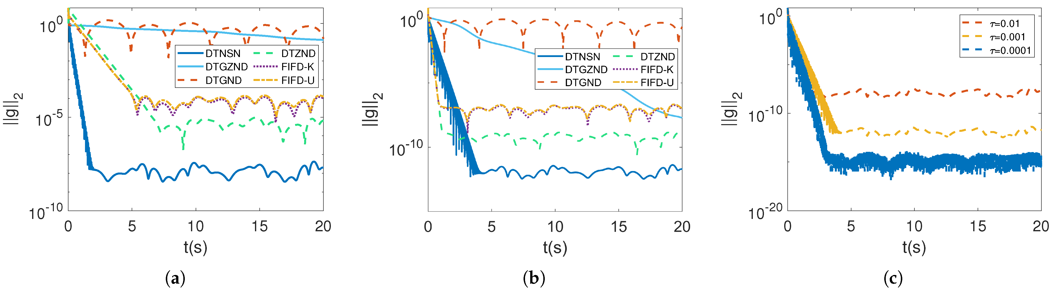
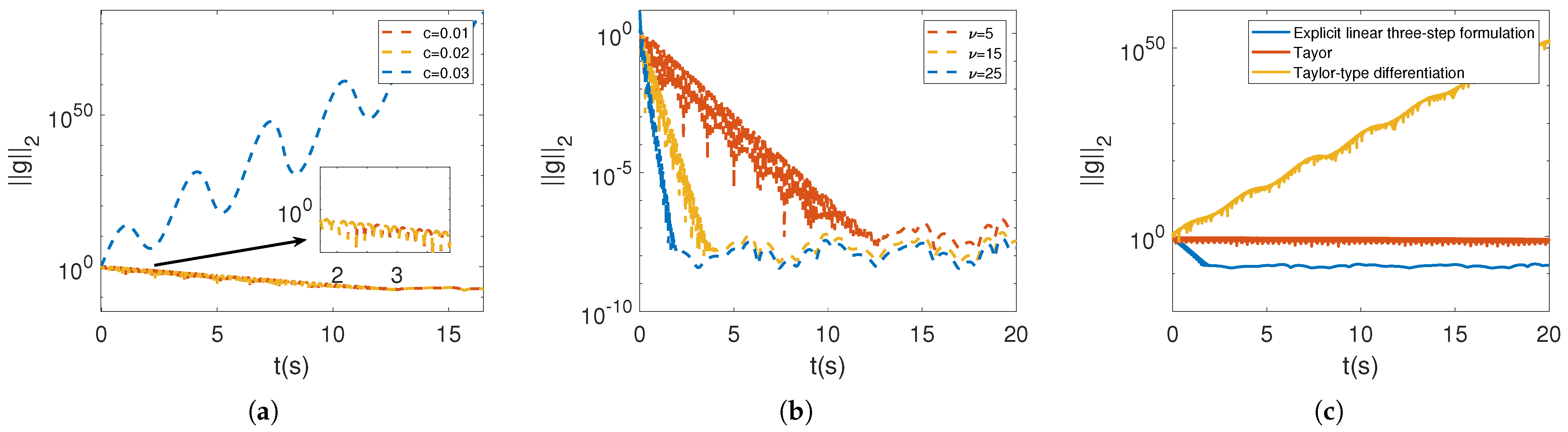
4.1. Comparison of Performance in a Noiseless Environment

This section presents four examples to test the convergence of the DTNSN model (13).

Example 1.

Consider the following general nonlinear optimization problem with time-varying linear equation constraints:

$$\begin{array}{cc}\hfill & min(sin\left(0.1t\right)+2)x_1^2+(cos\left(0.1t\right)+2)x_2^2+2cos\left(t\right)x_1{x}_2+sin\left(t\right)x_1+cos\left(t\right)x_2,\hfill \\ \hfill & \mathrm{s}.\mathrm{t}.sin\left(0.2t\right)x_1+cos\left(0.2t\right)x_2=cos\left(t\right).\hfill \end{array}$$

(33)

The aforementioned time-varying linear equation constraints are expressed as follows:

$$S\left(t\right)=[sin(0.2t),cos(0.2t\left)\right]\mathrm{and}\mathbf{q}\left(t\right)=cos\left(t\right).$$

As demonstrated in Figure 2a, when $\tau =0.01\mathrm{s}$, the DTNSN model (13) proposed in this paper achieves significantly higher convergence accuracy and shorter convergence time compared with other models. Notably, the relationship between sampling interval and performance exhibits interesting dynamics. While reducing $\tau$ to $0.001\mathrm{s}$ improves the convergence of residuals across all models (Figure 2b), the DTNSN model (13) maintains its competitive edge with consistently better convergence characteristics. This observation aligns with the trend shown in Figure 2c: specifically, smaller sampling intervals $\tau$ in the DTNSN model (13) lead to progressively higher convergence accuracy. This superiority is further corroborated by

Table 1. Comparison of different models for solving nonlinear optimization with time-varying equation constraints.

Model	EDI	Hyperparameters	MSSRE
			Without Noise	With CN	With TVLN	With RBN
DTGZND (15)	Yes	$\lambda$	$1.33\times {10}^{-1}$	$9.27\times {10}^{-2}$	$7.50\times {10}^{-2}$	$5.47\times {10}^{-2}$
DTGND (16)	No	$\lambda$	$1.48\times {10}^{-2}$	$7.82\times {10}^{-2}$	$7.58\times {10}^{-3}$	$2.33\times {10}^{-2}$
DTZND (17)	Yes	$\lambda$	$1.80\times {10}^{-7}$	$3.60\times {10}^{-1}$	$5.86\times {10}^{-2}$	$1.05\times {10}^{-1}$
FIFD-K (20)	Yes	$\kappa$	$5.17\times {10}^{-6}$	$1.80\times {10}^0$	$1.80\times {10}^0$	$1.80\times {10}^0$
FIFD-U (21)	No	$\kappa$	$1.10\times {10}^{-5}$	$1.80\times {10}^0$	$1.80\times {10}^0$	$1.80\times {10}^0$
DTNSN (13)	Yes	$\lambda ,\nu$	$3.15\times {10}^{-9}$	$3.51\times {10}^{-9}$	$2.94\times {10}^{-4}$	$3.51\times {10}^{-9}$

MSSRE represents maximum steady-state residual error. EDI represents exploiting derivative information. Parameters are produced by $\tau =0.01\mathrm{s}$, $\lambda =2,\nu =25$. CN indicates constant noise $\mathit{\vartheta }\left(t\right)={[5,5,5]}^T$, TVLN indicates time-varying linear noise $\mathit{\vartheta }\left(t\right)=0.5t{[1,1,1]}^T$, and RBN indicates random bounded noise $\mathit{\vartheta }\left(t\right)\in {[1,2]}^3$.

, which indicates that in noise-free environments, the error of our DTNSN model (13) in solving problem (33) is at least an order of magnitude lower than those of alternative models. However, it should be noted that this enhanced precision comes at a temporal cost—diminishing $\tau$ values proportionally extend the required convergence time.

In addition, the choice of appropriate parameters also significantly improves the convergence of the model. As can be seen from Figure 3a, the model has the best convergence performance when $\mathrm{c}=0.02$, and the maximum steady-state error is slightly better than that when $\mathrm{c}=0.03$. Moreover, the choice of appropriate hyperparameter $\nu$ also has a significant improvement on the convergence of the model. Figure 3b illustrates that the most expeditious convergence and the optimal convergence accuracy are attained when $\nu$ is set to 25. Furthermore, the choice of a reasonable discretization has an important impact on solving the problem. Figure 3c shows that the convergence accuracy of the DTNSN model (13) in solving problem (33) is better than other discretization methods. Not only does tuning the parameters affect the performance, but when discretizing the NSN model (10), which uses an explicitly three-step method, the model is significantly more accurate compared with other discretization methods.

The superiority of the linear three-step discretization method (12) has been shown in Figure 3c. Therefore, we carry out ablation experiments on the DTNSN model in addition to the discretization method. Figure 4a shows that the DTNSN model (13) with the integral feedback term has higher convergence accuracy than the DTGZND model (15) without it. The DTGND model (16), which lacks the time-varying tracking capability of ZND, also has lower convergence accuracy than the DTNSN model. Moreover, the DTZND (17) model, which does not use the gradient information of GND, has lower convergence speed than the DTNSN model.

Example 2.

Consider the following 2D nonlinear optimization problem with time-varying linear equation constraints:

$$\begin{array}{cc}\hfill & min{\displaystyle \frac{1}{2}}{\mathbf{x}}^{\mathrm{T}}\left(t\right)H_1\left(t\right)\mathbf{x}\left(t\right)+{\mathbf{r}}_1^{\mathrm{T}}\left(t\right)\mathbf{x}\left(t\right),\hfill \\ \hfill & \mathrm{s}.\mathrm{t}.S_1\left(t\right)\mathbf{x}\left(t\right)={\mathbf{q}}_1\left(t\right).\hfill \end{array}$$

(34)

where

$$H_1\left(t\right)=\left[\begin{array}{cc}sin\left(0.2t\right)+2& cos\left(0.1t\right)\\ cos\left(0.1t\right)& sin\left(0.2t\right)+4\end{array}\right]$$

and ${\mathbf{r}}_1\left(t\right)={[sin(t/10),sin(t/5)+1]}^{\mathrm{T}}$. The aforementioned time-varying linear equation constraints are expressed as follows:

$$S_1\left(t\right)=[cos\left(0.5t\right),sin\left(0.5t\right)]\mathit{and}{\mathbf{q}}_1\left(t\right)=sin\left(0.2t\right).$$

Example 3.

Consider the following 4D nonlinear optimization problem with time-varying linear equation constraints:

$$\begin{array}{cc}\hfill & min{\displaystyle \frac{1}{2}}{\mathbf{x}}^{\mathrm{T}}\left(t\right)H_2\left(t\right)\mathbf{x}\left(t\right)+{\mathbf{r}}_2^{\mathrm{T}}\left(t\right)\mathbf{x}\left(t\right),\hfill \\ \hfill & \mathrm{s}.\mathrm{t}.S{\left(t\right)}_2\mathbf{x}\left(t\right)={\mathbf{q}}_2\left(t\right).\hfill \end{array}$$

(35)

where

$$H_2\left(t\right)=\left[\begin{array}{cccc}{\displaystyle \frac{2}{5}}sin\left({\displaystyle \frac{2}{5}}t\right)+4& 1& sin\left({\displaystyle \frac{1}{5}}t\right)& 0\\ 1& {\displaystyle \frac{4}{5}}cos\left({\displaystyle \frac{1}{5}}t\right)+3& 1& 1\\ sin\left({\displaystyle \frac{1}{5}}t\right)& 1& {\displaystyle \frac{6}{5}}sin\left({\displaystyle \frac{2}{5}}t\right)+4& {\displaystyle \frac{1}{5}}cos\left({\displaystyle \frac{2}{5}}t\right)+1\\ 0& 1& {\displaystyle \frac{1}{5}}cos\left({\displaystyle \frac{2}{5}}t\right)+1& {\displaystyle \frac{4}{5}}cos\left({\displaystyle \frac{2}{5}}t\right)+3\end{array}\right]$$

and ${\mathbf{r}}_2\left(t\right)={\left[sin\left({\displaystyle \frac{2}{5}}t\right),sin\left({\displaystyle \frac{1}{5}}t\right)+1,cos\left({\displaystyle \frac{1}{5}}t\right)+2,sin\left({\displaystyle \frac{3}{5}}t\right)+1\right]}^{\mathrm{T}}$. The aforementioned time-varying linear equation constraints are expressed as follows:

$$S_2\left(t\right)=[cos\left(0.2t\right),sin\left(0.2t\right),sin\left(0.2t\right),cos\left(0.2t\right)]\mathit{and}{\mathbf{q}}_2\left(t\right)=sin\left(0.1t\right).$$

Example 4.

Consider the following 6D nonlinear optimization problem with time-varying linear equation constraints:

$$\begin{array}{cc}\hfill & min{\displaystyle \frac{1}{2}}{\mathbf{x}}^{\mathrm{T}}\left(t\right)H_3\left(t\right)\mathbf{x}\left(t\right)+{\mathbf{r}}_3^{\mathrm{T}}\left(t\right)\mathbf{x}\left(t\right),\hfill \\ \hfill & \mathrm{s}.\mathrm{t}.S_3\left(t\right)\mathbf{x}\left(t\right)={\mathbf{q}}_3\left(t\right).\hfill \end{array}$$

(36)

where

$$\begin{array}{cc}& H_3\left(t\right)=\left[{\mathbf{u}}_1\left(t\right),{\mathbf{u}}_2\left(t\right),{\mathbf{u}}_3\left(t\right),{\mathbf{u}}_4\left(t\right),{\mathbf{u}}_5\left(t\right),{\mathbf{u}}_6\left(t\right)\right],\hfill \\ & {\mathbf{u}}_1\left(t\right)={\left[{\displaystyle \frac{4}{t^2+4}}+6,0,{\displaystyle \frac{1}{2}}sin\left({\displaystyle \frac{1}{4}}t\right),0,1,{\displaystyle \frac{1}{4}}arctan\left({\displaystyle \frac{1}{5}}t\right)\right]}^{\mathrm{T}}\hfill \\ & {\mathbf{u}}_2\left(t\right)={\left[0,2,0,{\displaystyle \frac{1}{2}}cos\left({\displaystyle \frac{1}{5}}t\right),0,{\displaystyle \frac{1}{5}}sin\left({\displaystyle \frac{1}{4}}t\right)\right]}^{\mathrm{T}}\hfill \\ & {\mathbf{u}}_3\left(t\right)={\left[{\displaystyle \frac{1}{2}}sin\left({\displaystyle \frac{1}{4}}t\right),0,sin\left({\displaystyle \frac{1}{4}}t\right)+4,1,{\displaystyle \frac{1}{2}}sin\left({\displaystyle \frac{1}{4}}t\right),1\right]}^{\mathrm{T}}\hfill \\ & {\mathbf{u}}_4\left(t\right)={\left[0,{\displaystyle \frac{1}{2}}cos\left({\displaystyle \frac{1}{5}}t\right),1,4,{\displaystyle \frac{1}{2}}cos\left({\displaystyle \frac{1}{5}}t\right),0\right]}^{\mathrm{T}}\hfill \\ & {\mathbf{u}}_5\left(t\right)={\left[1,0,{\displaystyle \frac{1}{2}}sin\left({\displaystyle \frac{1}{4}}t\right),{\displaystyle \frac{1}{2}}cos\left({\displaystyle \frac{1}{5}}t\right),cos\left({\displaystyle \frac{1}{4}}t\right)+4,{\displaystyle \frac{4}{t^2+4}}\right]}^{\mathrm{T}}\hfill \\ & {\mathbf{u}}_6\left(t\right)={\left[{\displaystyle \frac{1}{4}}arctan\left({\displaystyle \frac{1}{5}}t\right),{\displaystyle \frac{1}{5}}sin\left({\displaystyle \frac{1}{4}}t\right),1,0,{\displaystyle \frac{4}{t^2+4}},6\right]}^{\mathrm{T}}\hfill \end{array}$$

and

$${\mathbf{r}}_3\left(t\right)={\left[1,sin\left({\displaystyle \frac{1}{5}}t\right),2,cos\left({\displaystyle \frac{1}{2}}t\right),sin\left({\displaystyle \frac{1}{5}}t\right)+1,1\right]}^{\mathrm{T}}.$$

The aforementioned time-varying linear equation constraints are expressed as follows:

$$S_3\left(t\right)=[sin\left(0.2t\right),cos\left(0.2t\right),sin\left(0.2t\right),cos\left(0.2t\right),sin\left(0.2t\right),cos\left(0.2t\right)]\mathrm{and}{\mathbf{q}}_3\left(t\right)=sin\left(0.5t\right).$$

The DTNSN model is valid for nonlinear optimization problems with different types of time-varying equation constraints. In Figure 2a and Figure 5, the DTNSN model successfully solves a general problem and time-varying quadratic programming problems containing time-varying equation constraints of 2D, 4D, and 6D with small steady-state errors, which confirms the convergence accuracy and stability of the DTNSN model (13).

4.2. Performance Comparison in Noisy Environments

In this section, an attempt is made to verify the robustness of the DTNSN model (13). To this end, different noise disturbances are introduced into problem (33), the results of which are presented in Figure 6.

4.2.1. Constant Noise Disturbance

In Figure 6a, the proposed DTNSN model still has superior convergence speed and convergence accuracy under constant noise disturbance ($\mathit{\vartheta }\left(t\right)={[5,5,5]}^T$). Conversely, if other models are subjected to constant noise disturbance, the majority of them will diverge and be incapable of effectively solving nonlinear optimization with time-varying equality constraints. Moreover, in Figure 4b, the convergence accuracy of the DTNSN model is stable under the interference of progressively larger constant noise, showing the good noise suppression capability of the DTNSN model.

4.2.2. Time-Varying Linear Noise Disturbance

From Figure 6b, it is clear that the convergence accuracy of the proposed DTNSN model is of class ${10}^{-4}$, which can well solve the time-varying linear noise $\mathit{\vartheta }\left(t\right)={[5,5,5]}^T$ under the nonlinear problems with time-varying equation constraints. Moreover, the proposed DTNSN model has good convergence accuracy and shielding against time-varying linear noise in comparison with the performance of other models.

4.2.3. Random Bounded Noise Disturbance

In Figure 6c, the presented DTNSN model maintains high accuracy under the interference of random noise $\mathit{\vartheta }\left(t\right)\in {[1,2]}^3$, and can be converged to ${10}^{-9}$ in a short period and remain stable. Other models converge up to ${10}^{-2}$ orders, after which they diverge and do not meet the criteria for engineering applications. Therefore, the proposed DTNSN model has superior convergence ability and robustness.

Additionally, Table 1 presents a summary of the key distinctions among different models under various noise disturbances.

4.3. Example Simulation of Acoustic Source Localization in IIOT

This subsection presents a simulation example of acoustic source localization for the Industrial Internet of Things (IIOT) using the proposed DTNSN model. The goal is to achieve real-time, ultra-accurate localization of a moving target via the time-difference-of-arrival (TDOA) method. In IIOT (Figure 7a), identification and tracking techniques are crucial. TDOA is a commonly used method. As per [21], the TDOA algorithm (Figure 7b) estimates a position by considering signal propagation speed and sensor coordinates. It calculates the time difference of signals received by different sensors. This precisely determines the signal source position, effectively solving the position estimation problem.

In the real world, this method is extensively applied across diverse localization domains. In this example, experiments on 3D acoustic source localization are conducted. The theoretical trajectory of the source is defined as ${\mathbf{P}}^{*}\left(t\right)$, which is expressed by the equation

$${\mathbf{P}}^{*}\left(t\right)=\left[\begin{array}{c}10sin\left(t\right)·cos\left(10t\right)\hfill \\ 10sin\left(t\right)·sin\left(10t\right)\hfill \\ 10cos\left(t\right)\hfill \end{array}\right]\in {\mathbb{R}}^3.$$

Additionally, the coordinates of the n acoustic transducers utilized for signal reception are denoted by the equation

$${\mathbf{R}}^{*}\left(t\right)=\left[\begin{array}{c}10sin\left(t_1\right)·cos\left(10t_1\right)\hfill \\ 10sin\left(t_1\right)·sin\left(10t_1\right)\hfill \\ 10cos\left(t_1\right)\hfill \\ \cdots \hfill \\ 10sin\left(t_n\right)·cos\left(10t_n\right)\hfill \\ 10sin\left(t_n\right)·sin\left(10t_n\right)\hfill \\ 10cos\left(t_n\right)\hfill \end{array}\right].$$

The time difference between other sensors and the target sensor is defined as ${\gamma }_j$, and the distance of each sensor in the 3D coordinate system is denoted by $d_j^2=x_j^2+y_j^2+z_j^2$. Thus, the distance difference between each sub-sensor and the target sensor is calculated as the product of the time difference between their arrival times (${\gamma }_j$) and the speed of sound propagation ($\upsilon$), i.e., $\Delta r_j=\upsilon {\gamma }_j$.

Ten acoustic sensors are considered. Utilizing the time differences ${\gamma }_j$ and the constant sound speed $\upsilon$, the equation for calculating the distance differences between each sensor and the target sensor is expressed as follows:

$$\begin{array}{c}\hfill \left[\begin{array}{ccc}{S}_{x_1}-S_{x_0}& S_{y_1}-S_{y_0}& S_{z_1}-S_{z_0}\\ ⋮& ⋮& ⋮\\ S_{x_n}-S_{x_0}& S_{y_n}-S_{y_0}& S_{z_n}-S_{z_0}\end{array}\right]\left[\begin{array}{c}x\left(t\right)\\ y\left(t\right)\\ z\left(t\right)\end{array}\right]=\left[\begin{array}{c}{l}_1-r_0\Delta r_1\\ ⋮\\ l_n-r_0\Delta r_n\end{array}\right],\end{array}$$

(37)

where $j\in \{1,2,\dots ,n\}$ and $l_j={\displaystyle \frac{d_j^2-d_0^2-\Delta r_j^2}{2}}$.

(37) can be written as the following linear equation:

$$\mathbf{S}\left(t\right)\mathbf{X}\left(t\right)=\mathbf{M}\left(t\right).$$

(38)

Therefore, it could be assumed that $\mathbf{E}\left(t\right)=\mathbf{S}\left(t\right)\mathbf{X}\left(t\right)-\mathbf{M}\left(t\right)$. Therefore, using the DTNSN model (13) to solve this problem can be formulated as

$$\begin{array}{c}\hfill {\mathbf{X}}_{k+1}=2{\mathbf{X}}_k-{\displaystyle \frac{3}{2}}{\mathbf{X}}_{k-1}+{\displaystyle \frac{1}{2}}{\mathbf{X}}_{k-2}+\tau \left({\displaystyle \frac{35}{24}}{\dot{\mathbf{X}}}_k-{\displaystyle \frac{5}{3}}{\dot{\mathbf{X}}}_{k-1}+{\displaystyle \frac{17}{24}}{\dot{\mathbf{X}}}_{k-2}\right),\end{array}$$

(39)

in which ${\dot{\mathbf{X}}}_k=-\lambda \left({\mathbf{S}}_k^{\mathrm{T}}{\mathbf{E}}_k\right)+{\mathbf{S}}_k^{-1}·\left(-\left({\dot{\mathbf{S}}}_k{\mathbf{X}}_k-{\dot{\mathbf{M}}}_k\right)-\nu {\sum }_{i=0}^k{\mathbf{E}}_i\right).$ Therefore, using the DTNSN model (13) to solve the above TDOA problem (37), we can simulate the image shown in Figure 8. As shown in Figure 8a, the predicted trajectories highly coincide with the actual trajectories in the noise-free case, which proves the ultra-accuracy of the DTNSN model (15). As can be seen in Figure 8b, the residuals along the x, y, and z axes converge to zero quickly and remain stable in the noise-free case. In addition, under constant noise interference, the predicted trajectory still closely matches the actual trajectory, as shown in Figure 8c. Figure 8d shows that even with some oscillation, the residuals along the x, y, and z axes quickly converge to zero. Furthermore, we also use the Kalman filter [42] for sound source localization. As can be seen from Figure 8e, the Kalman filter cannot precisely locate. Figure 8f also indicates that there is a relatively large error in using the Kalman filter for sound source location. This further highlights the good convergence properties and better robustness of the DTNSN model (13).

5. Conclusions and Future Work

This paper investigates solutions for time-varying nonlinear optimization with equation constraints and addresses practical challenges in noisy environments. Initially, the noise-suppressed neurodynamics (NSN) model is proposed as a solution to address the aforementioned problem. The convergence of the NSN model is rigorously guaranteed through theoretical proof. Subsequently, the NSN model is discretized via an explicitly linear three-step discretization method, yielding the discrete-time noise-suppressed neurodynamics (DTNSN) model. The global convergence and robustness of the DTNSN model are numerically validated in the presence of diverse noise disturbances. Ultimately, the practicality and effectiveness of the DTNSN model are demonstrated through its successful application to the time-difference-of-arrival (TDOA) problem. In future research, DTNSN can be widely used in areas that require real-time optimization under dynamic constraints and noise disturbances, such as extending it to deal with inequality constraints or superposition constraints, or hierarchical constraints for coordinating trajectory planning or obstacle avoidance systems for distributed UAV clusters.The DTNSN model can also be generalized to complex-valued problems to extend its application areas.

References

1. Kizielewicz, B.; Sałabun, W. A New Approach to Identifying a Multi-Criteria Decision Model Based on Stochastic Optimization Techniques. Symmetry 2020, 12, 1551. [Google Scholar] [CrossRef]
2. Liu, C.; Gong, Z.; Teo, K.L.; Feng, E. Multi-objective optimization of nonlinear switched time-delay systems in fed-batch process. Appl. Math. Model. 2016, 40, 10533–10548. [Google Scholar] [CrossRef]
3. Almotairi, K.H.; Abualigah, L. Hybrid Reptile Search Algorithm and Remora Optimization Algorithm for Optimization Tasks and Data Clustering. Symmetry 2022, 14, 458. [Google Scholar] [CrossRef]
4. Cafieri, S.; Monies, F.; Mongeau, M.; Bes, C. Plunge milling time optimization via mixed-integer nonlinear programming. Comput. Ind. Eng. 2016, 98, 434–445. [Google Scholar] [CrossRef]
5. Li, G.; Shuang, F.; Zhao, P.; Le, C. An Improved Butterfly Optimization Algorithm for Engineering Design Problems Using the Cross-Entropy Method. Symmetry 2019, 11, 1049. [Google Scholar] [CrossRef]
6. Zhang, J.; Hong, L.; Liu, Q. An Improved Whale Optimization Algorithm for the Traveling Salesman Problem. Symmetry 2021, 13, 48. [Google Scholar] [CrossRef]
7. Baek, J.; Cho, S.; Han, S. Practical time-delay control with adaptive gains for trajectory tracking of robot manipulators. IEEE Trans. Ind. Electron. 2018, 65, 5682–5692. [Google Scholar] [CrossRef]
8. Andrei, N. An accelerated subspace minimization three-term conjugate gradient algorithm for unconstrained optimization. Numer. Algorithms 2014, 65, 859–874. [Google Scholar] [CrossRef]
9. Nosrati, M.; Amini, K. A new diagonal quasi-Newton algorithm for unconstrained optimization problems. Appl. Math. 2024, 69, 501–512. [Google Scholar] [CrossRef]
10. Wu, W.; Zhang, Y.; Tan, N. Adaptive ZNN Model and Solvers for Tackling Temporally Variant Quadratic Program with Applications. IEEE Trans. Ind. Inform. 2024, 20, 13015–13025. [Google Scholar] [CrossRef]
11. Chen, J.; Pan, Y.; Zhang, Y. ZNN Continuous Model and Discrete Algorithm for Temporally Variant Optimization with Nonlinear Equation Constraints via Novel TD Formula. IEEE Trans. Syst. Man Cybern. Syst. 2024, 54, 3994–4004. [Google Scholar] [CrossRef]
12. Kong, L.; He, W.; Yang, W.; Li, Q.; Kaynak, O. Fuzzy Approximation-Based Finite-Time Control for a Robot with Actuator Saturation Under Time-Varying Constraints of Work Space. IEEE Trans. Cybern. 2021, 51, 4873–4884. [Google Scholar] [CrossRef] [PubMed]
13. Xu, F.; Shen, T. Look-Ahead Prediction-Based Real-Time Optimal Energy Management for Connected HEVs. IEEE Trans. Veh. Technol. 2020, 69, 2537–2551. [Google Scholar] [CrossRef]
14. Xu, L.; Li, X.R.; Duan, Z.; Lan, J. Modeling and State Estimation for Dynamic Systems with Linear Equality Constraints. IEEE Trans. Signal Process. 2013, 61, 2927–2939. [Google Scholar] [CrossRef]
15. Suszyński, M.; Peta, K.; Černohlávek, V.; Svoboda, M. Mechanical Assembly Sequence Determination Using Artificial Neural Networks Based on Selected DFA Rating Factors. Symmetry 2022, 14, 1013. [Google Scholar] [CrossRef]
16. Jiang, Y.; Peng, Z.; Wang, J. Safety-Certified Multi-Target Circumnavigation with Autonomous Surface Vehicles via Neurodynamics-Driven Distributed Optimization. IEEE Trans. Syst. Man Cybern. Syst. 2024, 54, 2092–2103. [Google Scholar] [CrossRef]
17. Li, W.; Wu, H.; Jin, L. A Lower Dimension Zeroing Neural Network for Time-Variant Quadratic Programming Applied to Robot Pose Control. IEEE Trans. Ind. Inform. 2024, 20, 11835–11843. [Google Scholar] [CrossRef]
18. Xiao, L.; Li, X.; Cao, P.; He, Y.; Tang, W.; Li, J.; Wang, Y. A Dynamic-Varying Parameter Enhanced ZNN Model for Solving Time-Varying Complex-Valued Tensor Inversion with Its Application to Image Encryption. IEEE Trans. Neural Netw. Learn. Syst. 2024, 35, 13681–13690. [Google Scholar] [CrossRef]
19. Zhang, J.; Jin, L.; Cheng, L. RNN for Perturbed Manipulability Optimization of Manipulators Based on a Distributed Scheme: A Game-Theoretic Perspective. IEEE Trans. Neural Netw. Learn. Syst. 2020, 31, 5116–5126. [Google Scholar] [CrossRef]
20. Katsikis, V.N.; Mourtas, S.D.; Stanimirović, P.S.; Zhang, Y. Solving Complex-Valued Time-Varying Linear Matrix Equations via QR Decomposition with Applications to Robotic Motion Tracking and on Angle-of-Arrival Localization. IEEE Trans. Neural Netw. Learn. Syst. 2022, 33, 3415–3424. [Google Scholar] [CrossRef]
21. Jin, L.; Yan, J.; Du, X.; Xiao, X.; Fu, D. RNN for Solving Time-Variant Generalized Sylvester Equation with Applications to Robots and Acoustic Source Localization. IEEE Trans. Ind. Inform. 2020, 16, 6359–6369. [Google Scholar] [CrossRef]
22. Narendra, K.; Parthasarathy, K. Gradient methods for the optimization of dynamical systems containing neural networks. IEEE Trans. Neural Netw. 1991, 2, 252–262. [Google Scholar] [CrossRef] [PubMed]
23. Zhang, Y.; Yang, Y.; Ruan, G. Performance analysis of gradient neural network exploited for online time-varying quadratic minimization and equality-constrained quadratic programming. Neurocomputing 2011, 74, 1710–1719. [Google Scholar] [CrossRef]
24. Xu, F.; Li, Z.; Nie, Z.; Shao, H.; Guo, D. Zeroing Neural Network for Solving Time-Varying Linear Equation and Inequality Systems. IEEE Trans. Neural Netw. Learn. Syst. 2019, 30, 2346–2357. [Google Scholar] [CrossRef]
25. Zhang, Y.; Shi, Y.; Xiao, L.; Mu, B. Convergence and stability results of Zhang neural network solving systems of time-varying nonlinear equations. In Proceedings of the 2012 8th International Conference on Natural Computation, Chongqing, China, 29–31 May 2012; pp. 143–147. [Google Scholar]
26. Chen, J.; Pan, Y.; Li, S.; Zhang, Y. Design and Analysis of Reciprocal Zhang Neuronet Handling Temporally-Variant Linear Matrix-Vector Equations Applied to Mobile Localization. IEEE Trans. Emerg. Top. Comput. Intell. 2024, 8, 2065–2074. [Google Scholar] [CrossRef]
27. Tan, N.; Yu, P.; Zheng, W. Uncalibrated and Unmodeled Image-Based Visual Servoing of Robot Manipulators Using Zeroing Neural Networks. IEEE Trans. Cybern. 2024, 54, 2446–2459. [Google Scholar] [CrossRef]
28. Qiu, B.; Guo, J.; Mao, M.; Tan, N. A Fuzzy-Enhanced Robust DZNN Model for Future Multiconstrained Nonlinear Optimization with Robotic Manipulator Control. IEEE Trans. Fuzzy Syst. 2024, 32, 160–173. [Google Scholar] [CrossRef]
29. Li, W.; Zou, Y.; Ma, X.; Qiu, B.; Guo, D. Novel Neural Controllers for Kinematic Redundancy Resolution of Joint-Constrained Gough–Stewart Robot. IEEE Trans. Ind. Inform. 2024, 20, 4559–4570. [Google Scholar] [CrossRef]
30. Nguyen, H.; Olaru, S.; Gutman, P.; Hovd, M. Constrained control of uncertain, time-varying linear discrete-time systems subject to bounded disturbances. IEEE Trans. Autom. Control 2015, 60, 831–836. [Google Scholar] [CrossRef]
31. Gan, Z.; Salman, E.; Stanaćević, M. Figures-of-merit to evaluate the significance of switching noise in analog circuits. IEEE Trans. Very Large Scale Integr. (VLSI) Syst. 2015, 23, 2945–2956. [Google Scholar] [CrossRef]
32. Zhang, Y.; Li, Z. Zhang neural network for online solution of time-varying convex quadratic program subject to time-varying linear-equality constraints. Phys. Lett. A 2009, 373, 1639–1643. [Google Scholar] [CrossRef]
33. Fu, Z.; Zhang, Y.; Tan, N. Gradient-feedback Zhang neural network for unconstrained time-variant convex optimization and robot manipulator application. IEEE Trans. Ind. Inform. 2023, 19, 10489–10500. [Google Scholar] [CrossRef]
34. Li, J.; Mao, M.; Uhlig, F.; Zhang, Y. Z-type neural-dynamics for time-varying nonlinear optimization under a linear equality constraint with robot application. J. Comput. Appl. Math. 2018, 327, 155–166. [Google Scholar] [CrossRef]
35. Liufu, Y.; Jin, L.; Xu, J.; Xiao, X.; Fu, D. Reformative Noise-Immune Neural Network for Equality-Constrained Optimization Applied to Image Target Detection. IEEE Trans. Emerg. Top. Comput. 2021, 10, 973–984. [Google Scholar] [CrossRef]
36. Guo, J.; Qiu, B.; Hu, C.; Zhang, Y. Discrete-time nonlinear optimization via zeroing neural dynamics based on explicit linear multi-step methods for tracking control of robot manipulators. Neurocomputing 2020, 412, 477–485. [Google Scholar] [CrossRef]
37. Zhang, Z.; Zhang, Y. Design and experimentation of accelerationlevel drift-free scheme aided by two recurrent neural networks. IET Control Theory Appl. 2013, 7, 25–42. [Google Scholar] [CrossRef]
38. Sun, M.; Wang, Y. General five-step discrete-time Zhang neural network for time-varying nonlinear optimization. Bull. Malays. Math. Sci. 2020, 43, 1741–1760. [Google Scholar] [CrossRef]
39. Griffiths, D.F.; Higham, D.J. Numerical Methods for Ordinary Differential Equations: Initial Value Problems; Springer: Berlin/Heidelberg, Germany, 2010. [Google Scholar]
40. Qi, Y.; Jin, L.; Wang, Y.; Xiao, L.; Zhang, J. Complex-Valued Discrete-Time Neural Dynamics for Perturbed Time-Dependent Complex Quadratic Programming with Applications. IEEE Trans. Neural Netw. Learn. Syst. 2020, 31, 3555–3569. [Google Scholar] [CrossRef]
41. Jin, L.; Zhang, Y. Discrete-time Zhang neural network of O(τ3) pattern for time-varying matrix pseudoinversion with application to manipulator motion generation. Neurocomputing 2020, 142, 165–173. [Google Scholar] [CrossRef]
42. Grondin, F.; Michaud, F. Lightweight and optimized sound source localization and tracking methods for open and closed microphone array configurations. Robot. Auton. Syst. 2019, 113, 63–80. [Google Scholar] [CrossRef]
Figure 1. Model block diagram of DTNSN model.
Symmetry 17 00932 g001
Figure 2. For the time-varying nonlinear optimization with equation constraints (33), the DTNSN model (13), the DTGZND model (15), the DTGND model (16), the DTZND model (17), the FIFD-K model (20), and the FIFD-U model (21) are respectively employed to solve the issue. (a) represents the residuals g ( t ) 2 of the six models for solving problem (33), where τ = 0.01 s . (b) represents the residuals g ( t ) 2 of the six models for solving problem (33), where τ = 0.001 s . (c) represents the residuals g ( t ) 2 of the DTNSN model (13) for solving problem (33), where τ = 0.01 s , τ = 0.001 s , and τ = 0.0001 s .
Symmetry 17 00932 g002
Figure 3. (a) denotes the residual convergence of the DTNSN model in the absence of noise using different parameters c: c = 0.01 , c = 0.02 , and c = 0.03 , where τ = 0.01 s . (b) denotes the residual convergence of the DTNSN model in the absence of noise using different parameters ν : ν = 5, ν = 15, and ν = 25, where τ = 0.01 s . (c) For the NSN (10) model, we discretize each of the three discretizations using explicitly linear three-step (12), Taylor [40], and Taylor-type numerical discretization [41], and then use their models to solve problem (33).
Symmetry 17 00932 g003
Figure 4. (a) denotes the residual g ( t ) 2 in solving (33) using the DTNSN model (13), the DTGZND model (15), the DTGND-IN model (18), and the DTZND model (19), where τ = 0.01 s . (b) denotes the residual g ( t ) 2 convergence of the DTNSN model (13) for different constant noises: ϑ ( t ) = [ 5 , 5 , 5 ] T , ϑ ( t ) = [ 10 , 10 , 10 ] T , and ϑ ( t ) = [ 15 , 15 , 15 ] T , where τ = 0.01 s .
Symmetry 17 00932 g004
Figure 5. Problem (34), problem (35), and problem (36) were solved using the DTNSN model (13), the DTGZND model (15), the DTGND model (16), the DTZND model (17), the FIFD-K model (20), and the FIFD-U model (21), respectively. (a) represents the residuals g ( t ) 2 of the six models for solving problem (34), where τ = 0.01 s . (b) represents the residuals g ( t ) 2 of the six models for solving problem (35), where τ = 0.01 s . (c) represents the residuals g ( t ) 2 of the six models for solving problem (36), where τ = 0.01 s .
Symmetry 17 00932 g005
Figure 6. The six models start with the same initial state and τ = 0.01 s . (a) represents the convergence of the residuals g ( t ) 2 from different models under constant noise disturbance ( ϑ ( t ) = [ 5 , 5 , 5 ] T ). (b) represents the convergence of the residuals g ( t ) 2 from different models under time-varying noise disturbance ( ϑ ( t ) = 0.5 t [ 1 , 1 , 1 ] T ). (c) represents the convergence of the residuals g ( t ) 2 from different models under random bounded noise disturbance ( ϑ ( t ) [ 1 , 2 ] 3 ).
Symmetry 17 00932 g006
Figure 7. (a) Key technologies of IIOT. (b) TDOA 3D localization schematic. Four sensors, A, B, C, and D, are used to capture the information of the moving sound source, and accurate 3D localization is achieved by obtaining the time of arrival of the sound to each sensor, and calculating the time difference between the sound arriving at the other sensors and sensor A. The time difference between the sound arriving at the other sensors and sensor A is calculated, where r refers to the distance between each sensor and the moving sound source.
Symmetry 17 00932 g007
Figure 8. The proposed DTNSN model (13) and Kalman filter [42] solve the TDOA in 3D. In the figure, the positions of the acoustic sensors are marked with small blue circles, the actual motion trajectories of the sound sources are represented by black solid lines, the predicted trajectories are represented by red dashed lines, and the observed data are represented by green dots. (a) is an image of the predicted trajectory and the actual trajectory using the DTNSN model (13) in the absence of noise. (b) is the error between the predicted trajectory and the actual trajectory when using the DTNSN model (13) in the absence of noise, and the three curves represent the x, y, and z coordinate errors of the sound source, respectively. (c) is an image of the predicted trajectory and the actual trajectory using the DTNSN model (13) under constant noise interference ϑ ( t ) = 5 . (d) is the error between the predicted trajectory and the actual trajectory when using the DTNSN model (13) under constant noise interference ϑ ( t ) = 5 . (e) is an image of the predicted trajectory and the actual trajectory using the Kalman filter [42] in the absence of noise. (f) is the error between the predicted trajectory and the actual trajectory when using the Kalman filter [42] in the absence of noise.
Symmetry 17 00932 g008