Symmetry-Aware Dynamic Scheduling Optimization in Hybrid Manufacturing Flexible Job Shops Using a Time Petri Nets Improved Genetic Algorithm

Abstract

Dynamic scheduling in hybrid flexible job shops (HFJSs) presents a critical challenge in modern manufacturing systems, particularly under dynamic and uncertain conditions. These systems often exhibit inherent structural and behavioral symmetry, such as uniform machine–job relationships and repeatable event response patterns. To leverage this, we propose a time Petri nets (TPNs) model that integrates time and logic constraints, capturing symmetric processing and setup behaviors across machines as well as dynamic job and machine events. A transition select coding mechanism is introduced, where each transition node is assigned a normalized priority value in the range [0, 1], preserving scheduling consistency and symmetry during decision-making. Furthermore, we develop a symmetry-aware time Petri nets-based improved genetic algorithm (TPGA) to solve both static and dynamic scheduling problems in HFJSs. Experimental evaluations show that TPGA significantly outperforms classical dispatching rules such as Shortest Job First (SJF) and Highest Response Ratio Next (HRN), achieving makespan reductions of 23%, 10%, and 13% in process, discrete, and hybrid manufacturing scenarios, respectively. These results highlight the potential of exploiting symmetry in system modeling and optimization for enhanced scheduling performance.

1. Introduction

Job shop scheduling is a critical problem in manufacturing activities, which further evolves into the complex and constraint-intensive problem of flexible job shop scheduling (FJSP) in the field of intelligent manufacturing [1,2,3,4]. Traditional job shop scheduling entails each job consisting of one or more operations, where each operation is executed on a single machine and occurs only once. Moreover, the processing times are known, and there exists a sequential constraint among job operations. By strategically arranging the processing sequence of jobs on machines, optimization of one or more scheduling metrics can be achieved. However, the flexibility introduced in a flexible job shop intensifies the complexity, as an operation can be processed on multiple designated machines, rendering FJSP NP-hard [5]. Furthermore, the dynamic nature of hybrid flexible job shop environments, which combine characteristics of both process and discrete manufacturing, amplifies the impact of real-time uncertainties such as equipment failures and urgent job insertions. Compared with classical FJSP, hybrid systems exhibit higher complexity and variability, making dynamic scheduling not only more challenging but also more critical for ensuring timely and efficient production.

Many studies have investigated the dynamic flexible job shop scheduling problem (DFJSP) and proposed various methodologies. Liu et al. [6] presented a multi-objective multi-population genetic algorithm for solving classical FJSP; however, this approach does not consider hybrid manufacturing environments or dynamic disruptions. Zhang et al. [7] devised a genetic programming hyperheuristic algorithm to address DFJSP with random machine failures, but the model lacks explicit time modeling for event handling. Baykasoğlu et al. [8] employed a greedy stochastic adaptive search for DFJSP with multiple dynamic events, which may suffer from poor scalability in complex hybrid shop floors. Li et al. [9] designed a modified Monte Carlo Tree Search algorithm to tackle DFJSP with four dynamic events, yet it does not integrate manufacturing logic and time constraints. Luo et al. [10] introduced a two-layer deep Q-network for optimizing average machine utilization and total weighted delay, but its effectiveness relies heavily on sufficient training data and lacks interpretability. To address DFJSP with limited transportation resources, Li et al. [11] proposed a hybrid deep Q-network aiming to minimize makespan and energy consumption, but it does not support generalized modeling for hybrid manufacturing types. Guo et al. [12] investigated DFJSP considering reconfigurable manufacturing cells (DFJSP-RMCs) and proposed an improved Genetic Programming Hyper-Heuristic (GPHH) method optimized for completion time, delay time, and reconfiguration time. Although this approach significantly reduces time consumption, it still lacks unified support for generalized hybrid manufacturing logic and time modeling. Furthermore, Yue et al. [13] considered dynamic events including new job insertion and random machine failures, and established a DFJSP optimization model tackled by a two-stage double deep Q-network (TS-DDQN). In addition, Chen et al. [14] proposed a Q-Learning-based NSGA-II (QNSGA-II) algorithm for DFJSP under transportation resource constraints, targeting makespan and energy consumption minimization while handling job cancellations, machine failures, and AGV breakdowns. An event-driven rescheduling strategy and a rescheduling instability index were introduced, alongside a hybrid initialization method and adaptive neighborhood selection to improve optimization performance. These approaches, while innovative, reveal a common limitation: they often lack unified frameworks capable of simultaneously modeling time, logic, and multiple manufacturing modes for dynamic scheduling in hybrid job shop environments.

Traditional flexible job shop scheduling primarily considers machine processing time in the manufacturing process. However, Ren et al. [15] and Zhang et al. [16] incorporated transmission time between machines when solving FJSP. To accommodate scheduling algorithms for job shop problems with additional constraints, researchers have integrated modeling methods such as Petri nets with the scheduling algorithms. Petri nets, conceptualized by Carl Adam Petri in the 1960s, have been extensively studied and widely adopted for modeling shop scheduling problems [17]. Wang et al. [18] proposed a new scheduling algorithm based on the position-timed Petri nets model and heuristic search to address scheduling problems in flexible manufacturing systems with deadlock susceptibility and no waiting constraints. Li et al. [19] introduced a heuristic method based on Petri nets and deep learning for FJSP. Zhao et al. [20] proposed an iterative greedy algorithm based on Petri nets for batch production FJSP. Hu et al. [21] utilized Petri nets to model manufacturing systems, avoiding deadlocks, and proposed a Petri net graph convolution layer employing deep Q-networks for solving dynamic scheduling problems in flexible job shops. Lassoued et al. [22] proposed PetriRL, a novel framework that integrates Petri nets and deep reinforcement learning (DRL) for optimizing job shop scheduling problems (JSSPs). This approach aims to improve productivity, reduce costs, and ensure timely delivery by leveraging the strengths of Petri nets in system modeling and DRL in adaptive decision-making.

As the manufacturing industry evolves, the job shop has transitioned from a single processing mode to a mixed manufacturing mode job shop with multiple processing modes [23]. Existing research methods typically consider a single time constraint, focusing solely on a single manufacturing mode. However, in addition to machine processing time, the adjustment of machine parameters is required when processing different products, known as setup time. Therefore, this paper aims to explore and propose a Petri nets model for a flexible job shop, along with a dynamic scheduling algorithm based on time Petri nets, intended to address these challenges.

The main contributions of this study, addressing the gaps identified above, are summarized as follows:

• We propose a symmetry-aware time Petri nets model for hybrid flexible job shop scheduling, integrating timing and logic constraints, which enables accurate representation of processing time, setup time, and real-time dynamic events.
• We propose a TPGA algorithm to address static and dynamic scheduling in hybrid environments. By introducing transition select coding to encode transition priorities, TPGA enables flexible scheduling under complex event-driven conditions.
• Experimental results show TPGA outperforms SJF and HRN, reducing makespan by 23%, 10%, and 13% in process, discrete, and hybrid manufacturing. These results confirm TPGA’s robustness and effectiveness under dynamic events.

The remainder of this article is organized as follows: Section 2 describes Petri nets, their notation, and their application to model hybrid manufacturing flexible job shop. The improved genetic algorithm is described in Section 3, including encoding, decoding, and algorithm execution. In Section 4, we present our experiments and results of our algorithm on standard and simulated datasets. Section 5 presents our conclusions and suggestions for future research.

2. Modeling of Hybrid Manufacturing Flexible Job Shop

This section first briefly introduces the basics of Petri nets, then the Petri nets model of the hybrid manufacturing flexible job shop.

2.1. Assumptions

To accurately model the flexible job shop scheduling problem (FJSP), the following assumptions and constraints are considered:

• All machines are assumed to be in a ready state at time zero.
• All jobs are in a ready state upon being introduced into the system.
• Each machine can process only one operation of one job at a time.
• Each operation must be processed on exactly one machine and only once.
• There is no priority constraint between operations of different jobs.
• Each job follows a predefined sequence of operations.
• No interruptions are allowed during the processing of any operation.

In addition, to describe the mathematical model of the FJSP, the following notation is defined in

Table 1. Notation used in the proposed FJSP model.

Notation	Description
n	Total number of jobs
m	Total number of machines
$O_{ij}$	The j-th operation of job i
$M_{ij}$	Set of machines capable of processing $O_{ij}$
$T_{ijk}$	Processing time of $O_{ij}$ on machine k
L	A sufficiently large positive number
$c_i$	Completion time of job i
$C_{max}$	Maximum completion time (makespan)
$S_{ijk}$	Start time of $O_{ij}$ on machine k
$F_{ijk}$	Finish time of $O_{ij}$ on machine k
$x_{ijk}$	$\left\{\begin{array}{cc}1,\hfill & \mathrm{if}{O}_{ij}\mathrm{is}\mathrm{processed}\mathrm{on}\mathrm{machine}k\hfill \\ 0,\hfill & \mathrm{otherwise}\hfill \end{array}\right.$
$y_{ijpqk}$	$\left\{\begin{array}{cc}1,\hfill & \mathrm{if}{O}_{ij}\mathrm{is}\mathrm{processed}\mathrm{before}{O}_{pq}\mathrm{on}\mathrm{machine}k\hfill \\ 0,\hfill & \mathrm{otherwise}\hfill \end{array}\right.$

:

2.2. Basics of Petri Nets

An ordinary Petri net is a three-tuple $N=(P,T,F)$, where P is a finite set of places, T is a finite set of transitions, and $F\subseteq (P\times T)\cup (T\times P)$ is the set of directed arcs. For a given node $x\in P\cup T$, its preset is defined as

$$•x=\left\{y\in P\cup T\left|\right(y,x)\in F\right\}$$

(1)

and postset

$$x•=\left\{y\in P\cup T\left|\right(x,y)\in F\right\}.$$

(2)

Let $Z=\left\{0,1,2,\dots \right\}$ and $Z_k=\left\{1,2,\dots ,k\right\}$. A string $\alpha =x_1,x_2\dots x_k$ is called a path in the Petri nets, where $x_i\in P\cup T$ and $(x_i,x_{i+1})\in F,i\in Z_{k-1}$.

A state or marking of N is a mapping $M:P\to Z$. Given a marking M and a place $p\in P$, denote $M\left(p\right)$ as the number of tokens in p at M. A Petri net N with an initial marking $M_0$ is called a marked Petri net, denoted by $(N,M_0)$.

A transition $t\in T$ is enabled at M if $\forall p\in •t,M\left(p\right)>0$. An enabled transition t can fire at M, yielding $M^{\prime }$, where $M^{\prime }\left(p\right)=M\left(p\right)+1$. A sequence of transitions $\alpha =t_1,t_2\dots t_k$ is feasible from M if there exists $M_i>M_{i+1},i\in Z_k$, where $M_1=M$.

A time Petri net is a four-tuple $TPN=(P,T,F,D)$, where D is a finite set of transition delays $d_t$ in the T set. In TPN, when a transition $t_i\in T$ is enabled, $M\left(p\right)$ tokens are extracted from the input place $p\in •t$ and transferred to the transition node $t_i$. After $d_{t_i}$ time units, add $M\left(p\right)$ tokens to the output place $p\in t•$. During this process, the fire transitions does not affect other transitions enabled, nor is it interrupted by other fire transitions.

A logic Petri net is a five-tuple $LPN=(P,T,F,f_I,f_O)$, and $f_I$ is the logical input function. For $\forall t\in T_I$, the logical input expression of the transition t is defined as

$$I_t=f_I\left(t\right)$$

(3)

Similarly, $f_O$ is the logical output function, where for $\forall t\in T_O$, the logical output expression of the transition t is defined as

$$O_t=f_O\left(t\right)$$

(4)

In LPN, for $\forall t\in T_I$, $I_t=f_I\left(t\right)$, if $•t$ satisfying the logical input expression $I_t$ under the marking M is true, then t is enabled at M. After t is fired, it yields a new marking $M^{\prime }$ given by the following rule, $\forall p\in •t$, if $M\left(p\right)=1$, then $M^{\prime }\left(p\right)=M\left(p\right)-1$; $\forall p\in t•,M^{\prime }\left(p\right)=M\left(p\right)+1$; $\forall p\notin •t\cup t•,M^{\prime }\left(p\right)=M\left(p\right)$. For $\forall t\in T_O$, $O_t=f_O\left(t\right)$, if $\forall p\in •t,M\left(p\right)=1$, then t is enabled at M. When t is fired, yielding $M^{\prime }$, where $M^{\prime }\left(p\right)=M\left(p\right)+1,\forall p\in •t,M^{\prime }\left(p\right)=M\left(p\right)\forall p\notin •t\cap t•$, for $p\in t•$ it should be satisfied that the logical input expression $O_t$ is true under the marking M.

The logic-time Petri net (TLPN) model proposed in this paper integrates the expressive logic control capability of logic Petri nets (LPNs) with the temporal modeling strength of time Petri nets (TPNs), forming a hybrid modeling framework that addresses dynamic and complex scheduling requirements in HMFJS. It can be formally defined as a six-tuple: $TLPN=(P,T,F,D,f_I,f_O)$, where P denotes places, T denotes transitions, F is the flow relation, D denotes time constraints, and $f_I$, $f_O$ represent input and output logic conditions, respectively. Unlike a conventional TPN, a TLPN enables transitions to be conditionally triggered through logical expressions involving machine states, job types, and resource readiness, while also embedding precise temporal delays. This dual capability allows the TLPN to more accurately capture the interplay between logical sequencing and time constraints in hybrid manufacturing systems.

2.3. Time Petri Nets Model of Hybrid Manufacturing Flexible Job Shop

The hybrid manufacturing flexible job shop (HMFJS) considered in this article comprises m types of machines, $M=\{m_i,i\in Z_m\}$, and is able to process n types of jobs, $Q=\{j_i,i\in Z_n\}$. More definitions and constraints are described as follows.

• The number of jobs $j_i$ to be processed is $\phi \left(j_i\right)$, and the total production of jobs to be processed is $\Phi =\begin{array}{c}{\sum }_{i\in Z_n}\phi \left(j_i\right)\end{array}$.
• Each machine is dedicated to a specific type of operation processing, with the count of each machine denoted as $\omega \left(m_i\right)$, and the total number of machines in the job shop is $\psi =\begin{array}{c}{\sum }_{i\in Z_m}\omega \left(m_i\right)\end{array}$.
• Jobs in the HMFJS are categorized as either process manufacturing jobs or discrete manufacturing jobs. A process manufacturing job consists of n sequential operations that must follow a strict linear order. In contrast, a discrete manufacturing job is composed of k components, where each component requires $n_i$, $i\in Z_k$ operations to process, and finally the components are processed into finished jobs by the combination operation.
• In the TLPN model, machines are modeled with distinct processing states reflecting the operation types they can execute. Transitions between these states incur setup times, which are explicitly modeled as timed transitions between corresponding places. For instance, when a machine switches from processing a component of a discrete job to a process manufacturing operation, a dedicated transition is triggered, guarded by a logical condition and associated with a setup delay (e.g., $d=5$ time units). This mechanism enables precise representation of real-world reconfiguration delays in dynamic scheduling decisions.
• The machine is in an unprocessed state at the beginning, and any type of operation at this time requires a certain amount of setup time.

According to the above constraints, we combine time Petri nets and logic Petri nets to establish the Petri nets model of the HMFJS. Places in our Petri nets model symbolize the state of an action or a resource. We utilize two types of places: simple place and action place. The simple place represents the resource, which in our model is represented as the state of the machine. The actions performed on a workstation (a group of machines of the same type), represented by the action place, illustrate the job’s processing state in the model. The process of machines’ processing jobs in the HMFJS is represented by transition nodes in our model. The machines in the job shop require different processing times for different jobs, and depending on the state of the machine, setup time may be required before processing. Therefore, a machine in the HMFJS has many different processing times. In our Petri nets model, each transition node has an associated time delay $d_t$, and a transition node represents an operation of a certain job to be processed on a certain machine. The time required is $d_t$. The mapping relationship between the concepts in the hybrid manufacturing flexible job shop and the elements in Petri nets is shown in

Table 2. The corresponding elements of a flexible job shop in Petri nets.

Flexible Job Shop	Elements in Petri Nets
Machine status	Place—simple
Job processing status	Place—action
Job processing	Transition nodes
Jobs quantity produced or moved	Directed arcs weight
Number of jobs that need to be completed	Number of tokens in place node representing job initial status
Number of jobs completed	Number of tokens in place node representing job completed status
Number of jobs being processed	Number of tokens in place node representing job operation status
Processing time of operation	Latency of transition nodes

.

As shown in Figure 1, the processing status of jobs and machines in the HMFJS is represented by place nodes in Petri nets. $P=\left\{p_{J_1{S}_1},p_{J_1{S}_2}\right\}$ represents the states before and after the processing of operation 1, respectively. $P=\left\{p_{M_1{J}_N},p_{M_1{J}_1},p_{M_1{J}_2},p_{M_1{J}_3},p_{M_1{J}_4}\right\}$ represents various processing states of machine 1. When machine 1 is processing job 1, the token representing the machine state is at the $p_{M_1{J}_1}$ node. Two different transition nodes are used to represent the operation of machine 1 processing job 1. $T_1$ is a time transition node associated with processing time T, which is the operation without setup time. $T_2$ is a logic time transition node, using the logic input expression $F_I=p_{J_1{S}_1}\wedge \left\{p_{M_1{J}_N}\vee p_{M_1{J}_2}\vee p_{M_1{J}_3}\vee p_{M_1{J}_4}\right\}$, which is the operation with setup time.

Example 1: Consider a flexible job shop that can process two types of process manufacturing jobs $j_1,j_2$. There are four machines, $m_1,m_2,m_3,m_4$, in the job shop. Among them, machines $m_1,m_3$, and $m_4$ can process both types of jobs, whereas machine $m_2$ is only capable of processing type 1 jobs. The operation route of $j_1$ is $m_1\to m_2\to m_4$ or $m_1\to m_3\to m_4$. The operation route of $j_2$ is $m_4\to m_3\to m_1$. According to the proposed Petri nets modeling method, the Petri nets model of the flexible job shop is shown in Figure 2a, where the number of tasks of $j_1$ and $j_2$ is 3 and 2.

Example 2: Consider a flexible job shop processing a discrete manufacturing operation $j_1$ consisting of two components. There are five machines, $m_1,m_2,m_3,m_4,m_5$, in the job shop. The two components of job $j_1$ are $p_1$ and $p_2$, respectively, the operation route of $p_1$ is $m_1\to m_3\to m_4$, and the operation route of $p_2$ is $m_2\to m_4$. Finally, the two components are combined into a complete product through $m_5$. According to the proposed Petri nets modeling method, the Petri nets model of the flexible job shop is shown in Figure 2b, where the number of tasks in $j_1$ is 3.

Example 3: After the original task is completed in the job shop scene of example 1, new tasks $j_1$ and $j_2$ are inserted, and the machine $m_2$ shuts down abnormally. According to the proposed Petri nets model, the dynamic events in the job shop are represented by modifying the number of tokens of the nodes in the established Petri nets model. As shown in Figure 2c, $M\left(p_{M_2{J}_N}\right)=1\to M\left(p_{M_2{J}_N}\right)=0$. The number of new tasks for $j_1$ and $j_2$ is 3. $M\left(p_{J_{1S}}\right)=0\to M\left(p_{J_{1S}}\right)=3,M\left(p_{J_{2S}}\right)=0\to M\left(p_{J_{2S}}\right)=3$.

Through example verification, the proposed time Petri nets model can be used to model process manufacturing jobs and discrete manufacturing jobs in the HMFJS. Our model helps the system avoid deadlocks by controlling requests for resources. The idea is that if granting a request for a resource may lead to a deadlock, then the request is not allowed to be valid. The transition nodes of the manufacturing process in the Petri net can only be fired when all input place conditions are met, and the emission of certain enabled transitions is intentionally controlled. Therefore, our model avoids deadlock scenarios by disrupting deadlock requests and hold conditions, ensuring a deadlock-free system. At the same time, the proposed model can represent the machine and job dynamic events in the job shop by modifying the number of resources in the nodes and provide a basis for dynamic scheduling.

3. TPGA for the DFJSP in Hybrid Manufacturing

A genetic algorithm (GA) has advantages in global and parallel searches, making it suitable for the discrete scheduling problems discussed in this paper. It also adapts well to flexible job shop scheduling and helps avoid local optima. However, standard GA does not explicitly consider time-related constraints and real-time dynamic events. To address this, we propose a Time Petri Nets Genetic Algorithm (TPGA), which integrates time Petri nets into a GA to handle both logic and timing constraints. The TPGA introduces transition select coding to prioritize transition firing, enabling adaptive scheduling in dynamic hybrid environments. This section details the chromosome coding/decoding schemes and the algorithm flow of the TPGA.

3.1. Chromosome Coding

The production process of the HMFJS is represented by the fire transition nodes in our Petri nets model. The job shop scheduling scheme can be expressed as a sequence of firing transitions starting from the initial marking state and leading to the end marking state in the Petri nets model. Transition-enabled constraints in the Petri nets model prevent any deadlock among the firing transition sequences acquired during the marking state transition process. Therefore, the TPGA proposed in this article encodes the transition nodes in the Petri net, which is called transition selection encoding. The transition select encoding assigns a random number between 0 and 1 to each transition node in the Petri nets model. The element in the chromosome is called a gene, where the value on the gene represents the priority of firing for transitions in the Petri nets model. Each gene corresponds to a transition in the constructed Petri nets model, and the chromosome length is equal to the number of transitions in the model. Specifically, for transitions that represent the same machining operation under different conditions (e.g., with or without preheating), only one gene is used to represent both, since they are mutually exclusive and do not require priority differentiation. As a result, the compressed chromosome length equals half the number of transitions in the original Petri net. This encoding approach preserves scheduling flexibility while reducing the solution space, thereby improving the efficiency of the genetic algorithm. To control randomness and ensure repeatability of experiments, all random number assignments are generated using a fixed pseudo-random seed. This guarantees that the same initial seed yields identical transition selection encodings, enabling deterministic benchmarking and fair algorithm comparisons.

The specific process of decoding starts from the initial marking state $M_0$, selecting one or more enabled transitions to fire it. The transition node promotes the change in the token in the place node, so that the Petri nets model moves toward the new marking state. Subsequently, one or more transitions enabled from the new marking state are fired to move the Petri net to the next marking state. Repeat the above steps until reaching the desired goal marking state. Among the enabled transitions, the fire transition node is selected based on the corresponding gene value encoded by each transition in the chromosome. Among the enabled transitions for any given marking, the transition with the lowest key value is selected and fired according to its encoding on the chromosome. Algorithm 1 describes the pseudo-code of the chromosome decoding process. The time complexity of the algorithm is $O(n·m^2)$. Here, n represents the maximum number of transitions required to transform the initial marking $M_0$ to the final marking $M_f$. Furthermore, m denotes the number of transitions in the Petri net. The algorithm consists of an outer loop and several inner loops. The outer loop runs up to n times. In each iteration, the dominant operation of the inner loop has a time complexity of $O\left(m^2\right)$. Combining these, the overall time complexity is derived as such. To avoid ambiguity, we provide the following clarification for line 5 in Algorithm 1: ${\sigma }_{fire}$ denotes the queue of currently activated transition nodes, and the if condition checks whether a transition in this queue has completed firing. Line 5 means that for each transition node that has completed firing, one token is added to each of its postset places to indicate that the transition has been successfully completed, thereby driving the further evolution of the model state.

Algorithm1: Decoding scheme

Example: Consider the Petri nets model of flexible job shop in process manufacturing as shown in Figure 2. The following chromosome is represented as an array of random keys [0.12, 0.05, 0.23, 0.98, 0.67, 0.78, 0.18, 0.54, 0.72, 0.11, 0.91, 0.79, 0.64, 0.45] associated, respectively, with transitions $\left[t_1,t_2,t_3,t_4,t_5,t_6,t_7,t_8,t_9,t_{10},t_{11},t_{12},t_{13},t_{14}\right]$.

Let the processing times of the transition node be $d_{t_1}=2,d_{t_2}=3,d_{t_3}=4,d_{t_4}=1,d_{t_5}=2,d_{t_6}=4,d_{t_7}=6,d_{t_8}=2,d_{t_9}=6,d_{t_{10}}=4,d_{t_{11}}=6,d_{t_{12}}=8,d_{t_{13}}=9,d_{t_{14}}=5$. The decoding process is written into

Table 3. The firing process of transitions based on current markings.

Step	Number of Tokens	Current Marking State	Transition Fired	Firing Transition Set
0	$M\left(p_{J1S}\right)=3,M\left(p_{J2S}\right)=2,M\left(p_{M1JN}\right)=1,$	$M_s$	–	${\sigma }_f=\left[t_2,t_{13}\right]$
	$M\left(p_{M2JN}\right)=1,M\left(p_{M3JN}\right)=1,M\left(p_{M4JN}\right)=1$
1	$M\left(p_{J1S}\right)=2,M\left(p_{J2S}\right)=2,M\left(p_{M1J1}\right)=1,$	$M_1$	$t_2$	${\sigma }_f=\left[t_{13}\right]$
	$M\left(p_{M2JN}\right)=1,M\left(p_{M3JN}\right)=1,M\left(p_{M4JN}\right)=1$
2	$M\left(p_{J1S}\right)=2,M\left(p_{J2S}\right)=1,M\left(p_{M1J1}\right)=1,$	$M_1$	$t_2,t_3$	${\sigma }_f=\left[t_1,t_6,t_7\right]$
	$M\left(p_{M2JN}\right)=1,M\left(p_{M3JN}\right)=1,M\left(p_{M4J2}\right)=1$

. The goal marking state $M_g$ requires $M\left(p_{J1E}\right)=3,M\left(p_{J2E}\right)=2$. The set of enabled transitions and their corresponding random keys (in parenthesis) are $t_2\left(0.05\right),t_{13}\left(0.64\right)$. Transition $t_2$ is to fire in 3 time units and $t_{13}$ is to fire in 9 time units. After 3 time units, $t_2$ releases tokens, the decoding continues until the goal marking is reached.

Decoding the above chromosome completely produces the following sequence of transition firings $\sigma =\left[t_2\&t_{13},t_1\&t_7,t_1\&t_6,t_8\&t_{14},t_9\&t_{12},t_3\&t_{10},t_{11},t_3,t_{11}\right]$, with $C_{max}=32$ corresponds to the makespan. To illustrate the effectiveness of the proposed TPGA, we compare its result with commonly used baseline heuristics. In the same scenario, the Shortest Job First (SJF) method results in a makespan of $C_{max}=34$. The Highest Response Ratio Next (HRN) method has not been evaluated in this example, but it can be incorporated in future work for further comparative analysis. This simulation case is self-constructed to demonstrate the logic and performance of the TLPN-based encoding and decoding framework.

3.2. A Genetic Algorithm Base on Time Petri Nets

Based on the Petri nets model in the previous section, a single-objective stable genetic algorithm is proposed. Algorithm 2 describes the pseudo-code of the TPGA. The time complexity of the algorithm is $O(k·nlogn)$. Here, n represents the size of the population, which is the number of individuals in the population used in the algorithm for the flexible job shop scheduling problem. The parameter k denotes the maximum number of iterations that the algorithm will run. The algorithm consists of an outer loop that executes up to k times. In each iteration, there is an inner loop that iterates approximately ${\displaystyle \frac{n}{2}}$ times. The dominant operations within each iteration of the outer loop include the operations in the inner loop and the sorting of the population based on fitness values. The sorting operation, which has a time complexity of $O(nlogn)$ for a population of size n, combined with the number of outer-loop iterations k. The objective function of the proposed TPGA is to minimize the maximum completion time, denoted as $C_{max}$, which represents the makespan of the entire scheduling process. Specifically, the TPGA aims to determine an optimal sequence of transition activations within the Petri nets model such that the last job finishes as early as possible. The mathematical formulation is defined as follows:

$$min{C}_{max}=\underset{j\in J}{max}\left\{C_j\right\}$$

(5)

where $C_j$ is the completion time of job j, and J is the set of all jobs. By minimizing $C_{max}$, the TPGA effectively optimizes the scheduling performance, improving system efficiency and reducing total production time.

In Algorithm 2, each individual in the population is coded using a transition select coding scheme as described previously. Lines 2 to 16 are the main loop. In this loop, if (1) they provide a better solution after decoding according to Algorithm 1, and if (2) they have not yet appeared in the population, new individuals are generated to replace the worst individuals. The main loop is repeated until the termination condition (time limit) is reached, and the population collection is returned.

In main loop, two individuals (parent individuals) are selected from the population by the tournament selection operator, and a single-point crossover operator is used to combine the information of the two individuals to generate a new individual. In this scheme, a random intersection point is chosen. The initial sub-solution is derived from the first part (before the cutoff point) of the first-parent individual and the second part from the second first-parent individual. Likewise, a second sub-solution is generated using the second part from the first first-parent individual and the first part from the second first-parent individual.

After the crossover operator, individuals are mutated with a given probability as an algorithm parameter. Using the crossover mutation algorithm, this operator selects two genes in a chromosome and swaps their positions. Through several times of exchange operations, the decoded scheduling scheme can be adjusted without changing the value of chromosome genes, and the change range of the scheduling scheme is positively correlated with the number of exchanges and the number of genes involved in each exchange process. Finally, the resulting population is examined, and the decoding algorithm is used to convert the solution of the population into a scheduling scheme.

Algorithm2: TPGA

4. Experimental Studies

4.1. Implementation Details

All algorithms in this article were implemented in Python3. The experiments were conducted in a computer with AMD Ryzen 9 4900HS CPU 3.0GHz processor, 16GB memory and Windows 11 operation system. To ensure that the randomness in the genetic algorithm did not affect the experimental results, the experimental cases were run 10 times, and the average value of the solution results was used as the experimental results to judge the performance of TPGA. The algorithm parameters are shown in

Table 4. The parameter settings of TPGA.

Parameter	Value
Number of individuals	300
Maximum iteration rounds	100
Crossover probability	0.8
Mutation probability	0.5

.

The experimental data in this section are divided into public datasets and simulation datasets. The public datasets used Lee’s job shop case 3, 4a, and 4b [24], referred to as LD3, LD4a, and LD4b in this article, respectively. LD3 is a small-scale case with 5 jobs and 6 machines, representing low scheduling complexity. LD4a is a medium-scale instance with 10 jobs and 10 machines, involving moderate flexibility and complexity. LD4b is a large-scale case with 15 jobs and 10 machines, characterized by a greater number of operations and higher routing flexibility, making it significantly more challenging. These cases were selected to simulate small-, medium-, and large-scale manufacturing scenarios, respectively. The public datasets are the flexible job shop scheduling problem under the ideal state. To demonstrate the practicality of our proposed algorithm in addressing the dynamic scheduling challenges of a hybrid manufacturing flexible job shop, we incorporated real production shop processes. Using Python, we simulated the hybrid manufacturing flexible job shop and set the static scheduling case and dynamic scheduling case of the hybrid manufacturing flexible job shop as the simulation datasets. The datasets were not entirely based on real-world production data. Instead, they consisted of a combination of open-source benchmark simulation data and datasets generated by simulating hybrid process and discrete manufacturing workflows inspired by actual production processes. For dynamic scheduling experiments, typical real-world scenarios such as job insertion events and machine breakdowns were simulated to enhance the practical relevance of the study.

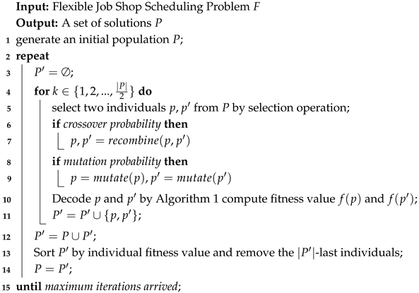
4.2. Results and Discussion

The case mentioned by Lee has been adopted by most scholars as the test standard of most Petri net algorithms. The classic algorithm and recently proposed graph search algorithms based on Petri nets are used as a comparison to verify the superiority of the algorithm. The five algorithms referenced in [24,25,26,27,28] are all graph-based scheduling methods utilizing Petri nets models. L1, DWS, and HFBS are heuristic-driven search algorithms based on firing sequence enumeration. ACAS and WGA incorporate adaptive control strategies and weighted evaluation metrics to improve scheduling outcomes. NSGA-II is a widely adopted multi-objective evolutionary algorithm. In contrast, the proposed TPGA approach integrates a time Petri nets model with a genetic algorithm framework, leveraging token dynamics to handle both static and dynamic scheduling under uncertainty.

In the comparative experiments, a set of predefined production tasks and workflows for flexible job shop systems are used as benchmark cases. Each task consists of a sequence of operations, and every operation has an associated work time. The performance metric reported in

Table 5. The results of LD case.

	L1	DWS	HFBS	ACAS	WGA	NSGA-II	TPGA
LD3	426	329	327	326	326	327	323
LD4a	298	254	253	253	246	249	245
LD4b	273	237	237	231	226	229	227

L1: Level-1 Algorithm; DWS: Dynamic Weight Search; HFBS: Heuristic Feature-Based Search; ACAS: Adaptive Cooperative Algorithm Strategy; WGA: Weighted Genetic Algorithm; NSGA-II: Non-dominated Sorting Genetic Algorithm II; TPGA: Time Petri Nets Improved Genetic Algorithm.

is the total completion time (makespan) required to finish all tasks in each case, measured in time units. A lower value indicates better scheduling performance.

From the comparative experimental results, it can be seen that with the minimum completion time as the optimization goal, the TPGA has obtained a better solution in the three cases. The stability of the TPGA’s results across repeated calculations indicates its ability to consistently provide superior solutions. The experimental results prove that the Petri nets method proposed in this article can accurately describe the manufacturing process of the flexible job shop, and the TPGA can effectively search for an excellent scheduling scheme on the Petri nets model. The effectiveness of the model and the proposed algorithm is verified.

In traditional flexible job shop scheduling problems, machine constraints typically account only for processing time. However, in real manufacturing settings, machines incur additional setup time when transitioning between different jobs for processing. These time constraints were not considered in the LD3, LD4a, and LD4b cases. In order to further demonstrate that the TPGA can still address the actual manufacturing scenario with multiple time constraints, we produced a simulation dataset with multiple time constraints for experiments.

We set up experimental cases of different scales in process manufacturing scenarios, discrete manufacturing scenarios and hybrid manufacturing scenarios. The size of the experimental case was determined by the number of job types and the number of machine types in the job shop. The job shop in the experimental case was modeled by the Petri nets modeling method proposed in this article, and the TPGA was used on the model to address the flexible job shop scheduling problem. In order to evaluate the performance of the TPGA, the greedy iterative algorithms SJF and HRN were used to address the flexible job shop scheduling problem on the established model.

After multiple tests with a population size of 300, the algorithm typically required 30 to 60 iterations to obtain a stable and improved solution. The maximum number of iterations was set to 100, and the algorithm running time was about 150 s.

In a process manufacturing scenario, jobs are processed by different types of machines in a job shop in a fixed sequence. In the small-scale case, the job shop has five types of machines and four types of jobs, and each job is processed by three to five operations. In the medium-scale case, the job shop has eight types of machines, six types of jobs, and each type of jobs is processed by six to eight operations. In a large-scale case, the job shop has ten types of machines, ten types of jobs, and each type of job is processed by seven to ten operations. In the experimental case, five of each type of jobs need to be produced, and there are three of each type of machine in the job shop. The experimental results are shown in

Table 6. Scheduling results for the flexible job shop scheduling case with multiple time constraints.

Scenes	Case	(Job, Machine)	SJF	HRN	TPGA
Process manufacturing	PM1	(4, 5)	376	392	310
	PM2	(4, 5)	553	553	448
	PM3	(6, 8)	709	598	531
	PM4	(6, 8)	769	740	611
	PM5	(10, 10)	1465	1216	1061
	PM6	(10, 10)	1368	1330	1087
Discrete manufacturing	DM1	(4, 5)	961	893	756
	DM2	(4, 5)	801	810	685
	DM3	(6, 8)	1097	1024	928
	DM4	(6, 8)	1014	940	874
	DM5	(10, 10)	1802	1880	1669
	DM6	(10, 10)	2215	2009	1920
Hybrid manufacturing	HM1	(4, 5)	663	570	506
	HM2	(4, 5)	512	466	414
	HM3	(6, 8)	764	830	676
	HM4	(6, 8)	651	636	542
	HM5	(10, 10)	1309	1213	1076
	HM6	(10, 10)	1333	1270	1147

. In the process manufacturing scenario, the TPGA has achieved a better scheduling results across all scales. Due to the low complexity of process manufacturing operations, changes in the scale of the job shop have little impact on the TPGA’s performance. As shown in Figure 3, in the process manufacturing scenario, the performance of the TPGA is improved by an average of 20% compared with the greedy iterative algorithm.

In a discrete manufacturing scenario, a job consists of two to three components. Each component is completed in a fixed processing sequence, and finally, the assembly machine combines the components into a complete job. In the small-scale case, the job shop has five types of machines, four types of jobs, and the components of the jobs are processed by three to five operations. In the medium-scale case, the job shop has eight types of machines, six types of jobs, and the components of the jobs are processed by four to six operations. In a large-scale case, the job shop has ten types of machines, ten types of jobs, and the parts of the jobs are processed by five to eight operations. In the experimental case, five of each job type need to be produced. There are three processing machines of each type in the job shop, and the number of assembly machines is five. The experimental results are shown in Table 6. In the discrete manufacturing scenario, the TPGA still obtains better results at various scales, but with the increase in the job shop scale, the solution efficiency and quality of the TPGA decrease. This is because discrete manufacturing operations are relatively complex, and the scale of the job shop has a greater impact on the solution space of the algorithm. As shown in Figure 3, compared with the greedy iterative algorithm, the performance of the TPGA is improved by an average of 15% in the discrete manufacturing scenario.

In a hybrid manufacturing scenario, the job shop has both the above-mentioned process manufacturing jobs and discrete manufacturing jobs. In the experimental case, the number of jobs in the two processing processes is the same, there are three processing machines of each type in the workshop, and the number of assembly machines is five. The experimental results are shown in Table 6. In hybrid scenarios, job shop scheduling exhibits higher complexity. The performance of the HRN algorithm fluctuates significantly at different scales, whereas the TPGA consistently achieves better scheduling results across various scales. As shown in Figure 3, compared with the greedy iterative algorithm, the performance of TPGA is improved by 18% on average in the discrete manufacturing scenario.

In order to verify the dynamic scheduling performance of the algorithm proposed in this paper, we add random dynamic events to different scales of process manufacturing, discrete manufacturing, and hybrid manufacturing cases. Dynamic events are divided into three categories: job events, machine events, and hybrid events.

Job events are those events which temporarily add the jobs to the job shop. Select 3–6 types of jobs from the existing pool of six types to increase their number. The incremented count ranges randomly between 4 and 6. Machine events are used to reduce the number of machines at the job shop workstations. Random machine events are introduced across the five types of machines in the workshop, where the number of faults for each machine type is random. At least three machines of each type are kept available. Hybrid events refer to job events and machine events occurring simultaneously. These events add tasks for 3–6 types of jobs in the workshop, introducing random task quantities ranging from three to six, implementing random machine events across the five types of machines, and randomizing the number of faults for each machine type. A minimum of four machines for each type is ensured to remain operational.

Machine events lead to changes in the job shop’s job processing capabilities and require dynamic adjustment of the scheduling plan. Job events simulate random job insertion events that occur in the real job shop and randomizing the number of faults for each machine type. A minimum of four machines for each type is ensured to remain operational. The TPGA employs event-driven rescheduling to adapt the scheduling method to dynamic events and utilizes a complete rescheduling strategy for all unprocessed and new jobs.

The experimental results of the dynamic scheduling case of the hybrid manufacturing job shop are shown in

Table 7. Scheduling results of flexible job shop dynamic scheduling case in hybrid manufacturing.

Case	(Job, Machine)	Job Event			Machine Event			Hybrid Event
		SJF	HRN	TPGA	SJF	HRN	TPGA	SJF	HRN	TPGA
PM1	(4, 5)	260	279	203	320	346	246	420	400	305
PM3	(6, 8)	498	498	434	559	435	394	780	639	574
PM5	(10, 10)	1127	1069	863	1024	957	767	1558	1432	1260
DM1	(4, 5)	747	812	692	648	599	553	844	784	736
DM3	(6, 8)	900	844	784	959	957	904	1125	1157	1094
DM5	(10, 10)	1416	1528	1277	1470	1416	1240	2032	2207	1919
HM1	(4, 5)	621	591	494	509	507	424	606	561	519
HM3	(6, 8)	610	697	512	630	638	581	777	843	745
HM5	(10, 10)	1200	1166	1030	1295	1299	1179	1403	1352	1278

. All algorithms were run 10 times continuously in process manufacturing and discrete manufacturing scenarios, respectively, and the average values were used for comparison. The TPGA achieves the best scheduling results for three dynamic events in different scenarios. In the dynamic flexible job shop case study, three manufacturing types (process, discrete, and hybrid) and three scales (small, medium, large) were considered. 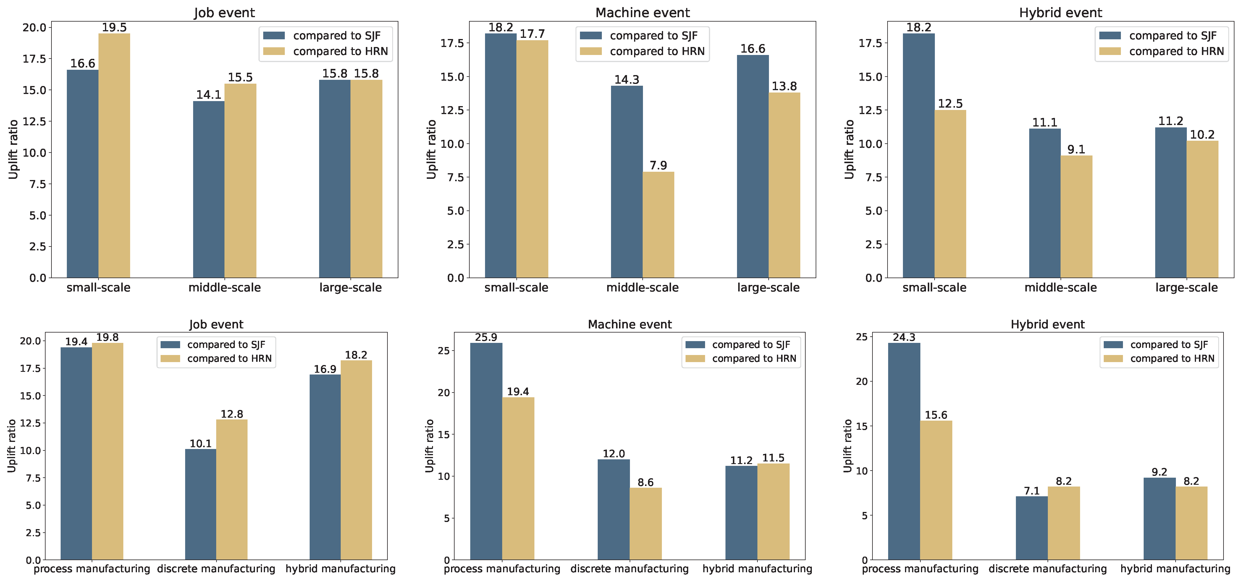Figure 4 shows the efficiency improvement of the proposed algorithm over SJF and HRN under three dynamic event types: job, machine, and hybrid events. The first row presents results by manufacturing scale, and the second row by manufacturing type. Captions and legends clearly distinguish the dynamic event types. Compared to the greedy iterative algorithm, the proposed method improves average performance by 23% in process manufacturing. The discrete manufacturing flexible job shop has higher job complexity, and the dynamic scheduling performance of the TPGA in this scenario is improved by an average of 10%. The hybrid manufacturing job shop has both features of process manufacturing and discrete manufacturing. The TPGA improves the dynamic scheduling problem results of hybrid manufacturing flexible job shop by an average of 13% compared with the greedy iterative algorithm. As shown in Figure 4, the TPGA has superior performance compared with the greedy iterative algorithm in solving the small-scale flexible job shop dynamic scheduling problem.

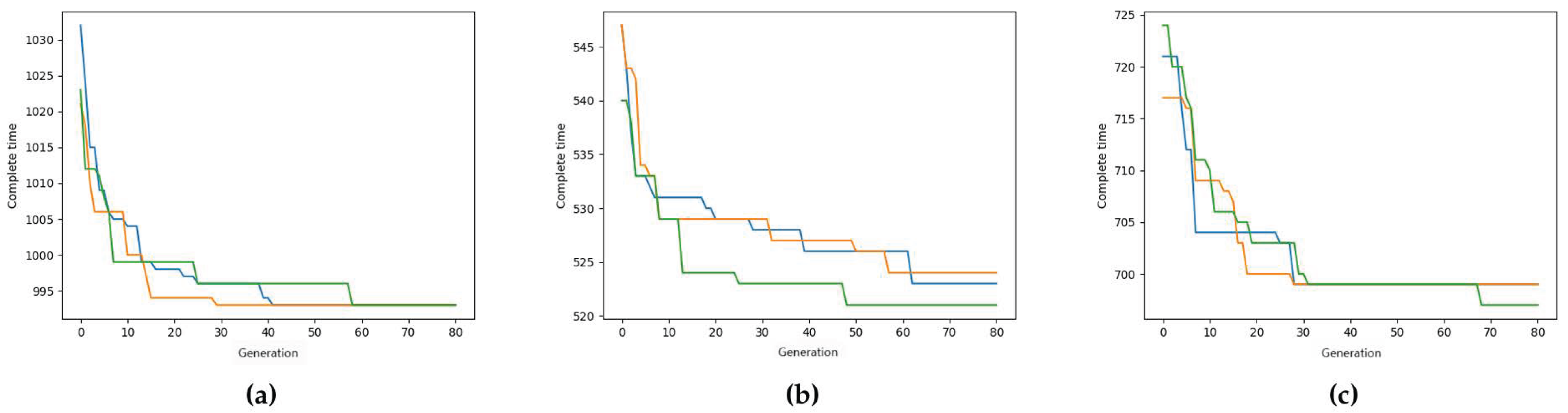
In addition, we have also conducted some experiments to test the convergence speed of the proposed algorithm. In the experiment, 100 flexible job shop scenarios were generated through simulation. All cases were tested using the Time Petri Nets Improved Genetic Algorithm. The algorithm includes three main parameters: population size, crossover probability, and mutation probability. During testing, two parameters were fixed while the third was varied. Representative cases were selected to visualize the impact of parameter adjustments on algorithm performance. Figure 5 displays the convergence curves of completion time across generations for selected representative cases. Each colored line corresponds to a different parameter setting. The curves demonstrate that completion time decreases with generations and stabilizes, indicating the algorithm’s ability to converge toward optimal or near-optimal solutions over iterations.

From these experiments, we can see that the proposed algorithm is very effective for solving dynamic and static scheduling problems of multiple time-constrained flexible job shops in hybrid manufacturing mode. The TPGA has the advantages of good adaptability and strong search ability in various scenarios. It can produce better results in both simple and complex scenarios.

5. Practical Implications

The proposed Time Petri Nets Genetic Algorithm (TPGA) provides a promising approach for enhancing real-time scheduling performance in dynamic and complex job shop environments. Due to its inherent ability to model both temporal constraints and event-driven disruptions (e.g., new job arrivals or machine failures), the TPGA can be effectively embedded into real-time production control systems. Specifically, the TPGA can serve as a scheduling engine within Manufacturing Execution Systems (MESs) or Industrial Internet of Things (IIoT) platforms, where sensor data and system feedback are continuously integrated to trigger rescheduling actions.

For practitioners and operations managers, the TPGA offers several practical advantages. First, its dynamic token-based mechanism enables real-time response to unexpected events, ensuring minimal production interruption. Second, the modularity of the Petri nets structure allows for customized modeling of diverse production layouts, including process, discrete, and hybrid manufacturing. Third, the TPGA can help improve key performance indicators (KPIs) such as machine utilization, on-time delivery rate, and system flexibility.

To facilitate deployment, the algorithm can be implemented in a distributed computing environment where scheduling decisions are periodically updated based on the latest shop floor data. Visualization tools can also be integrated to help managers interpret Petri net states and make informed decisions in real time. These capabilities position the TPGA as a practical and adaptable solution for modern smart manufacturing systems.

6. Conclusions

This study investigates the dynamic flexible job shop scheduling problem (DFJSP) in hybrid manufacturing environments and proposes a novel scheduling approach based on a flexible job shop Petri nets model combined with a Time Petri Nets Genetic Algorithm (TPGA). The proposed model effectively integrates processing and setup time constraints by utilizing place and transition nodes and dynamically handles unpredictable job insertions and machine breakdowns through token operations.

To evaluate the performance of the TPGA, we conducted comparative experiments against classical dispatching rules, including Shortest Job First (SJF) and Highest Response Ratio Next (HRN), under three different manufacturing modes: process, discrete, and hybrid. The results demonstrate that the TPGA outperforms the benchmarks in terms of makespan. Specifically, the TPGA achieved makespan reductions of 23%, 10%, and 13% in process, discrete, and hybrid manufacturing scenarios, respectively. These quantifiable improvements highlight the effectiveness of the TPGA in addressing scheduling challenges in dynamic environments.

Despite these encouraging results, some limitations remain. First, the model assumes deterministic processing and setup times, which may not fully capture the uncertainty inherent in real-world manufacturing environments. Second, the complexity of the Petri nets structure could grow significantly with larger-scale job shops, potentially introducing computational challenges. Third, the current study focuses on single-objective optimization (minimizing makespan), while actual manufacturing settings often require balancing multiple conflicting objectives such as cost, energy consumption, and delivery deadlines.

In future work, we plan to extend this research in several directions. One is to explore multi-objective optimization using improved versions of the Petri nets model. Another promising direction is to incorporate stochastic factors and real-time data to better model uncertainty. Additionally, we aim to investigate the application of the Petri nets framework in job completion time forecasting, thereby enhancing its potential for real-time production monitoring and decision-making.

References

1. Fang, Y.; Peng, C.; Lou, P.; Zhou, Z.; Hu, J.; Yan, J. Digital-twin-based job shop scheduling toward smart manufacturing. IEEE Trans. Ind. Inform. 2019, 15, 6425–6435. [Google Scholar] [CrossRef]
2. Zhang, F.; Mei, Y.; Nguyen, S.; Zhang, M. Correlation coefficient-based recombinative guidance for genetic programming hyperheuristics in dynamic flexible job shop scheduling. IEEE Trans. Evol. Comput. 2021, 25, 552–566. [Google Scholar] [CrossRef]
3. Li, R.; Gong, W.; Lu, C. Self-adaptive multi-objective evolutionary algorithm for flexible job shop scheduling with fuzzy processing time. Comput. Ind. Eng. 2022, 168, 108099. [Google Scholar] [CrossRef]
4. Peng, Z.; Zhang, H.; Tang, H.; Feng, Y.; Yin, W. Research on flexible job-shop scheduling problem in green sustainable manufacturing based on learning effect. J. Intell. Manuf. 2021, 33, 1725–1746. [Google Scholar] [CrossRef]
5. Destouet, C.; Tlahig, H.; Bettayeb, B.; Mazari, B. Flexible job shop scheduling problem under Industry 5.0: A survey on human reintegration, environmental consideration and resilience improvement. J. Manuf. Syst. 2023, 67, 155–173. [Google Scholar] [CrossRef]
6. Liu, S.C.; Chen, Z.G.; Zhan, Z.H.; Jeon, S.W.; Kwong, S.; Zhang, J. Many-objective job-shop scheduling: A multiple populations for multiple objectives-based genetic algorithm approach. IEEE Trans. Cybern. 2021, 53, 1460–1474. [Google Scholar] [CrossRef]
7. Zhang, F.; Mei, Y.; Nguyen, S.; Zhang, M. Evolving scheduling heuristics via genetic programming with feature selection in dynamic flexible job-shop scheduling. IEEE Trans. Cybern. 2020, 51, 1797–1811. [Google Scholar] [CrossRef]
8. Baykasoğlu, A.; Madenoğlu, F.S.; Hamzadayı, A. Greedy randomized adaptive search for dynamic flexible job-shop scheduling. J. Manuf. Syst. 2020, 56, 425–451. [Google Scholar] [CrossRef]
9. Li, K.; Deng, Q.; Zhang, L.; Fan, Q.; Gong, G.; Ding, S. An effective MCTS-based algorithm for minimizing makespan in dynamic flexible job shop scheduling problem. Comput. Ind. Eng. 2021, 155, 107211. [Google Scholar] [CrossRef]
10. Luo, S.; Zhang, L.; Fan, Y. Dynamic multi-objective scheduling for flexible job shop by deep reinforcement learning. Comput. Ind. Eng. 2021, 159, 107489. [Google Scholar] [CrossRef]
11. Li, Y.; Gu, W.; Yuan, M.; Tang, Y. Real-time data-driven dynamic scheduling for flexible job shop with insufficient transportation resources using hybrid deep Q network. Robot.-Comput.-Integr. Manuf. 2022, 74, 102283. [Google Scholar] [CrossRef]
12. Guo, H.; Liu, J.; Wang, Y.; Zhuang, C. An improved genetic programming hyper-heuristic for the dynamic flexible job shop scheduling problem with reconfigurable manufacturing cells. J. Manuf. Syst. 2024, 74, 252–263. [Google Scholar] [CrossRef]
13. Yue, L.; Peng, K.; Ding, L.; Mumtaz, J.; Lin, L.; Zou, T. Two-stage double deep Q-network algorithm considering external non-dominant set for multi-objective dynamic flexible job shop scheduling problems. Swarm Evol. Comput. 2024, 90, 101660. [Google Scholar] [CrossRef]
14. Chen, R.; Wu, B.; Wang, H.; Tong, H.; Yan, F. A Q-Learning based NSGA-II for dynamic flexible job shop scheduling with limited transportation resources. Swarm Evol. Comput. 2024, 90, 101658. [Google Scholar] [CrossRef]
15. Ren, W.; Yan, Y.; Hu, Y.; Guan, Y. Joint optimisation for dynamic flexible job-shop scheduling problem with transportation time and resource constraints. Int. J. Prod. Res. 2022, 60, 5675–5696. [Google Scholar] [CrossRef]
16. Zhang, G.; Hu, Y.; Sun, J.; Zhang, W. An improved genetic algorithm for the flexible job shop scheduling problem with multiple time constraints. Swarm Evol. Comput. 2020, 54, 100664. [Google Scholar] [CrossRef]
17. Kabir, S.; Papadopoulos, Y. Applications of Bayesian networks and Petri nets in safety, reliability, and risk assessments: A review. Saf. Sci. 2019, 115, 154–175. [Google Scholar] [CrossRef]
18. Wang, X.; Xing, K.; Feng, Y.; Wu, Y. Scheduling of flexible manufacturing systems subject to no-wait constraints via Petri nets and heuristic search. IEEE Trans. Syst. Man Cybern. Syst. 2019, 51, 6122–6133. [Google Scholar] [CrossRef]
19. Li, J.; Luo, J.; Li, X.; Yi, S.; Pan, C. Heuristic Scheduling Method for FMSs Based on P-timed Petri Nets and Deep Learning. In Proceedings of the 2022 IEEE International Conference on Networking, Sensing and Control (ICNSC), Shanghai, China, 15–18 December 2022; pp. 1–6. [Google Scholar]
20. Zhao, Z.; Liu, S.; Zhou, M.; You, D.; Guo, X. Heuristic scheduling of batch production processes based on Petri nets and iterated greedy algorithms. IEEE Trans. Autom. Sci. Eng. 2022, 19, 251–261. [Google Scholar] [CrossRef]
21. Hu, L.; Liu, Z.; Hu, W.; Wang, Y.; Tan, J.; Wu, F. Petri-net-based dynamic scheduling of flexible manufacturing system via deep reinforcement learning with graph convolutional network. J. Manuf. Syst. 2020, 55, 1–14. [Google Scholar] [CrossRef]
22. Lassoued, S.; Schwung, A. Introducing PetriRL: An innovative framework for JSSP resolution integrating Petri nets and event-based reinforcement learning. J. Manuf. Syst. 2024, 74, 690–702. [Google Scholar] [CrossRef]
23. Ocampo-Martinez, C. Energy efficiency in discrete-manufacturing systems: Insights, trends, and control strategies. J. Manuf. Syst. 2019, 52, 131–145. [Google Scholar]
24. Lee, D.Y.; DiCesare, F. Scheduling flexible manufacturing systems using Petri nets and heuristic search. IEEE Trans. Robot. Autom. 1994, 10, 123–132. [Google Scholar] [CrossRef]
25. Moro, A.R.; Yu, H.; Kelleher, G. Hybrid heuristic search for the scheduling of flexible manufacturing systems using Petri nets. IEEE Trans. Robot. Autom. 2002, 18, 240–245. [Google Scholar] [CrossRef]
26. Mejía, G.; Niño, K. A new Hybrid Filtered Beam Search algorithm for deadlock-free scheduling of flexible manufacturing systems using Petri Nets. Comput. Ind. Eng. 2017, 108, 165–176. [Google Scholar] [CrossRef]
27. Baruwa, O.T.; Piera, M.A. Identifying FMS repetitive patterns for efficient search-based scheduling algorithm: A colored Petri net approach. J. Manuf. Syst. 2015, 35, 120–135. [Google Scholar] [CrossRef]
28. Mejía, G.; Pereira, J. Multiobjective scheduling algorithm for flexible manufacturing systems with Petri nets. J. Manuf. Syst. 2020, 54, 272–284. [Google Scholar] [CrossRef]
Figure 1. Petri nets model of job operation in hybrid manufacturing flexible job shop.
Symmetry 17 00907 g001
Figure 2. (a) Petri nets model of flexible job shop in process manufacturing. (b) Petri nets model of flexible job shop in discrete manufacturing. (c) Petri nets model of process manufacturing flexible job shop after responding to dynamic events.
Symmetry 17 00907 g002
Figure 3. Scheduling performance improvement of TPGA compared with SJF and HRN algorithms under process, discrete, and hybrid manufacturing types.
Symmetry 17 00907 g003
Figure 4. Scheduling performance improvement of TPGA compared with SJF and HRN algorithms under different dynamic events for process, discrete, and hybrid manufacturing types.
Symmetry 17 00907 g004
Figure 5. (a) Convergence plot of TPGA algorithm under Case 1. (b) Convergence plot of TPGA algorithm under Case 30. (c) Convergence plot of TPGA algorithm under Case 50.
Symmetry 17 00907 g005