Homological Properties and Digital Relative Homology Groups of MA-Spaces

Abstract

This study investigates certain homological properties of Marcus–Wyse-based digital spaces, particularly the construction of digital relative homology groups and the excision property within MA-spaces. The Marcus–Wyse topology (for brevity M-) facilitates the definition of continuity, connectedness, and neighborhood relations in pixel-based spaces, thereby enabling the adaptation of algebraic topology methods to digital image data. Within this framework, the functorial structure of digital singular homology on MA-spaces is established, showing that homology groups can be defined and computed in a categorical setting. These results not only strengthen the theoretical foundation of digital topology but also contribute to practical applications such as topological feature extraction, image segmentation, and shape analysis in discrete environments.

1. Introduction

Topological structures constitute a foundational framework in the analysis and processing of digital images. In particular, locally finite topologies have proven beneficial in the study of digital spaces, where many image processing tasks rely heavily on specific notions of connectedness—most notably, 4-connectedness. Within this context, the M-topology provides a rigorous topological structure for discrete pixel spaces, enabling precise definitions of continuity, connectedness, and neighborhood relations [1,2,3,4]. Due to its inherent symmetry in local neighborhoods, the M-topology supports more efficient algorithmic computations and typically requires fewer boundary conditions compared to the more complex local structure of the Khalimsky topology [5]. Originally introduced by Marcus and Wyse in [6], this topology holds significant relevance in both theoretical and applied digital topology and was first utilized by Rosenfeld in the context of computer vision applications [7]. Klette [8] provides a comprehensive review of the use of M-topology in characterizing orthogonal planar grids, thereby clarifying their structural implications in digital image analysis. Beyond grid-based representations, advancements in computational topology have increasingly emphasized homology-based methods. Mrozek et al. [9] demonstrated the capability of homology algorithms to robustly extract one-dimensional features from noisy multidimensional data, while Assaf et al. [10] employed persistent homology for effective grayscale image segmentation. Ghrist [11] introduced barcodes to detect and analyze topological features in high-dimensional datasets. Peltier et al. [12] and Allili and Ziou [13] presented algorithmic methods for computing homology groups and extracting topological features across various imaging modalities. More recently, DelMarco [14] applied computational topology to vision-aided navigation in GPS-denied environments, and Edelsbrunner [15] provided further evidence of the value of persistent homology in quantifying topological structures in image processing. Collectively, these studies underscore both the utility of M-topology in grid representation and the effectiveness of homology-based approaches—including persistent and combinatorial techniques—for robust feature extraction, segmentation, and topology-aware image analysis. Beyond global topological frameworks, local properties such as adjacency relations play a crucial role in determining proximity and connectedness in digital grids. In [16], Eckhardt and Latecki established fundamental criteria for connectedness in the digital plane:

(i)

A subset of ${\mathbb{Z}}^2$ is (topologically) connected if it is 4-connected.

(ii)

A subset of ${\mathbb{Z}}^2$ is not (topologically) connected if it is not 8-connected.

These conditions are satisfied by the most widely adopted adjacency relations in computer vision and digital geometry. Topological invariants such as homology, homotopy, and cohomology provide robust tools for distinguishing and analyzing digital spaces [17,18,19]. In particular, relative homology enables the study of structural features of a space in relation to a specified subspace, thereby offering a more nuanced understanding of digital image topology. Arslan, Karaca, and Öztel [17] introduced a homological framework for n-dimensional digital images based on digital simplicial homology, extending classical topological methods into the discrete setting. Vergili and Karaca introduced the digital singular homology groups of the digital spaces [20]; later, they introduced relative homology groups for digital spaces endowed with the Khalimsky topology and investigated key properties such as the additivity and excision axioms within this setting [5]. Ege, Karaca, and Erden Ege [21] further explored the behavior of Eilenberg–Steenrod axioms in the context of digital simplicial homology, while a digital singular homology theory for MA-spaces was presented in [22].

Building upon these foundational contributions in digital topology and homology, this paper focuses on the analysis of features within digital image spaces via relative homology, while employing the M-topology to endow such spaces with a rigorous and meaningful topological structure. The principal objective of the present work is to examine specific topological properties of MA-spaces. In particular, I introduce digital relative homology groups for MA-spaces, demonstrate that the excision property holds in this setting, and establish that the homology functor $H_n$ defines a covariant functor from the category of MA-spaces (MAC) to the category of abelian groups (Ab). A significant structural aspect is that, due to the definition of simplices and the nature of MA-spaces, digital simplices ${\Delta }^n$ do not exist for $n\ge 2$. Thus, only 0- and 1-simplices occur in MA-spaces, which fundamentally shapes the homological framework and computational considerations in this setting.

The content of this paper is divided as follows. Some basic notions about the adjacency relations, M-topology, and digital singular homology are given in Section 2. Section 3 studies some properties of homology groups of MA-spaces such as the functorial property of digital singular homology on MA-spaces between the categories MAC and Ab. Section 4 introduces the digital relative homology groups of MA-spaces and studies some properties of digital relative homology groups by using the algebraic topological tools. Section 5 concludes the paper with a summary and possible further research.

2. Preliminaries

Let $\mathbb{Z}$ denote the set of integers. For any subset $X\subset {\mathbb{Z}}^n$ with a $\kappa$-adjacency, we call a pair $(X,\kappa )$ a digital image. As established in [18] (see also [23]), the $\kappa$-adjacency relations of ${\mathbb{Z}}^n$ are defined as follows: for a natural number l with $1\le l\le n$, two distinct points $p=(p_1,p_2,\dots ,p_n)\mathrm{and}q=(q_1,q_2,\dots ,q_n)\mathrm{in}{\mathbb{Z}}^n$ are considered ${\kappa }_l$-adjacent (or κ-adjacent) if the difference $|p_i-q_i|=1$ holds for at most l indices i, and $p_i=q_i$ for all other indices i.

Define a subset $B_M\left(p\right)\subset {\mathbb{Z}}^2$ for each $p=(p_1,p_2)\in {\mathbb{Z}}^2$ as

$$B_M\left(p\right):=\left\{\begin{array}{cc}\{(p_1\pm 1,p_2),p,(p_1,p_2\pm 1)\},\hfill & \mathrm{if}{p}_1+p_2\mathrm{is}\mathrm{even},\hfill \\ \left\{p\right\},\hfill & \mathrm{otherwise}.\hfill \end{array}\right.$$

(1)

The topology on ${\mathbb{Z}}^2$ induced by the set $\left\{B_M\left(p\right)\right|p\in {\mathbb{Z}}^2\}$ is called the Marcus–Wyse topology (M-topology for short) and is denoted by $({\mathbb{Z}}^2,\gamma )$ [6].

We recall the following definitions from [24]. For two distinct points $x,y\in ({\mathbb{Z}}^2,\gamma )$, if $y\in B_M\left(x\right)$ or $x\in B_M\left(y\right)$, the points x and y are said to be MA-adjacent.

Consider

$$MA\left(p\right):=\{q\in {\mathbb{Z}}^2|p\mathrm{and}q\mathrm{are}4-\mathrm{adjacent}\mathrm{with}\mathrm{respect}\mathrm{to}\mathrm{one}\mathrm{another}\}$$

for a point $p\in {\mathbb{Z}}^2$, and take $M{A}_X\left(p\right):=MA\left(p\right)\cap X$ for a space $(X,{\gamma }_X)$. If $p\in M{A}_X\left(q\right)$ or $q\in M{A}_X\left(p\right)$ where $p,q\in X(p\ne q)$, these two points are called M-adjacent to each other and the set $M{A}_X\left(p\right)\cup \left\{p\right\}:=M{N}_X\left(p\right)$ is called the MA-neighborhood of p in X.

We use the notation $(X,{\gamma }_X)$ to represent an M-topological space with an MA-adjacency, and call it an MA-space. Throughout the remainder of this paper, we shall refer to MA-spaces of the form $(X,{\gamma }_X)$ simply as X for notational simplicity.

Let X and Y be two MA-spaces. A function $f:X\to Y$ is called an MA-map at a point $x\in X$ if

$$f\left(MN\right(x\left)\right)\subset MN\left(f\right(x\left)\right).$$

(2)

Moreover, if the map $f:X\to Y$ is an MA-map at every point $x\in X$, then f is called an MA-map.

Remark 1 

([24]).

1. 

An MA-map preserves the M-connectedness. However, the converse does not hold.

2. 

The inverse map of a bijective MA-map does not need to be an MA-map.

A bijective, continuous MA-map that has a continuous inverse (which is also an MA-map) is called an MA-isomorphism [24].

If there is a path ${\left(p_i\right)}_{i\in {[0,m]}_{\mathbb{Z}}}$ on X from x to y with $x\ne y$, and $\{x_0=x,x_1,\dots ,x_m=y\}$ such that $\{p_i,p_{i+1}\}$ is MA-connected, $i\in {[0,m-1]}_{\mathbb{Z}},m>1$, we say x and y are MA-path connected; also, the number m is called the length of given MA-path. Moreover, if $x_0=x_m$, the MA-path is referred to as a closed MA-curve. A simple MA-path in a space X is defined as a finite sequence ${\left(x_i\right)}_{i\in {[0,m]}_{\mathbb{Z}}}$, where two points $x_i$ and $x_j$ are M-adjacent if and only if $|i-j|=1$. A simple closed MA-curve, also known as an MA-loop, is a simple MA-path of length l, denoted by ${\left(x_i\right)}_{i\in {[0,l]}_{\mathbb{Z}}}\subset {\mathbb{Z}}^n$, satisfying $x_0=x_l$ and the adjacency condition $x_i$ is M-adjacent to $x_j$ if and only if $|i-j|=1\left(modl\right)$. Such a curve is typically denoted by $S{C}_{MA}^l$ [24].

Let $(X,\kappa )$ be a digital image and S be a nonempty subset of X. The elements $s\in S$ are defined to be simplices of $(X,\kappa )$ [17] if the following conditions are met:

(i) 

Any distinct two points of S are $\kappa$-adjacent.

(ii) 

$t\in S$ whenever $\varnothing \ne t\subset s$ for $s\in S$.

A simplex with $n+1$ elements is called an n-simplex.

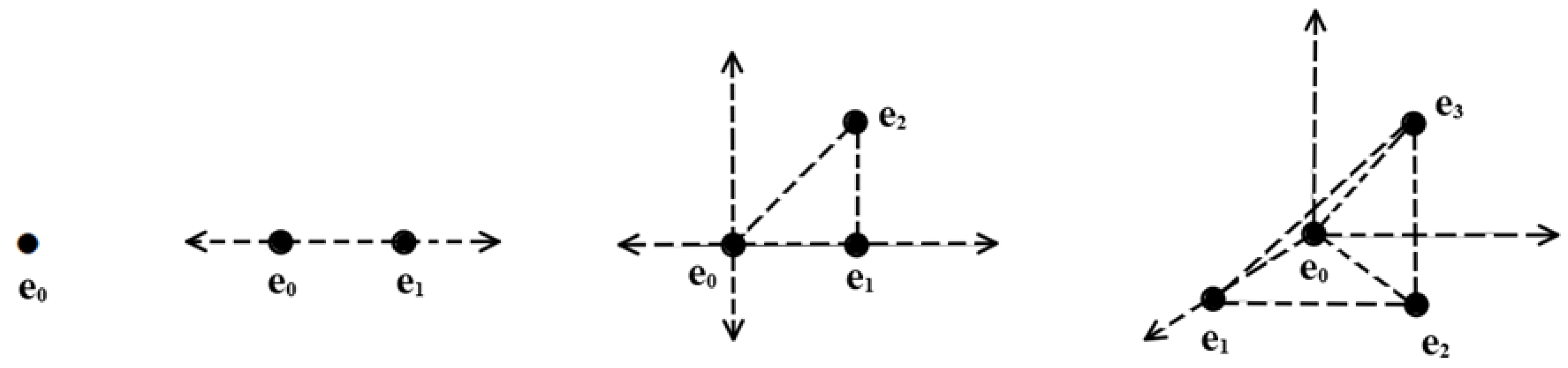
Let ${\Delta }^n=[e_0,e_1,\dots ,e_n]$ denote the digital standard n-simplex in ${\mathbb{Z}}^n$ [20] (see Figure 1) spanned by some specific points $e_0=(0,0,\dots ,0)$ and $e_i=(i_1,i_2,\dots ,i_n)$ for $1\le i\le n$ where

$$\begin{array}{c}\hfill i_m=\left\{\begin{array}{cc}1,\hfill & \mathrm{if}m\le i;\hfill \\ 0,\hfill & \mathrm{if}m>i.\hfill \end{array}\right.\end{array}$$

An orientation of ${\Delta }^n=[e_0,e_1,\dots ,e_n]$ refers to its vertices that are linearly ordered. The notation $-[e_0,\dots ,\widehat{e_i},\dots ,e_n]$ denotes the ith face vertex $e_i$ removed with an orientation opposite to the one where the vertices are ordered as presented (i.e., $e_0<e_1<\dots <e_n$). Subsequently, the induced orientation of its faces can be determined by orienting the ith face according to the arrangement ${(-1)}^i[e_0,\dots ,\widehat{e_i},\dots ,e_n]$ [22].

Remark 2 

([22]). According to the definition of a simplex and the structure of MA-spaces, n cannot be greater than or equal to 2 when ${\Delta }^n$ is equipped with the M-topology inherited from ${\mathbb{Z}}^n$. Thus, we only have 0- and 1-simplices in MA-spaces.

Definition 1 

([22]). An MA-map ${\sigma }^n:{\Delta }^n\to X$ for X an MA-space is called a digital singular n-simplex in X. $S_n\left(X\right)$ is defined to be a free abelian group with a basis consisting of all singular n-simplexes in X for each $n\ge 0$. The elements of $S_n\left(X\right)$ are called digital singular n-chains.

Definition 2 

([22]). The ith face map ${\epsilon }_i={\epsilon }_i^n:{\Delta }^{n-1}\to {\Delta }^n$ for each n and i is defined to be a map that takes the vertices $\{e_0,\dots ,e_{n-1}\}$ to the vertices $\{e_0,\dots ,\widehat{e_i},\dots ,e_n\}$ by preserving the displayed orderings.

Let X be an MA-space. The boundary of a digital singular n-simplex ${\sigma }^n:{\Delta }^n\to X$ is

$${\displaystyle {\partial }_n\sigma =\sum _{i=0}^n{(-1)}^i\sigma {\epsilon }_i^n\in S_{n-1}\left(X\right).}$$

${\partial }_0\sigma =0$ when $n=0$.

${\partial }_n:S_n\left(X\right)\to S_{n-1}\left(X\right)$ homomorphisms are called boundary operators. Since boundary operators are linear, there exists only one homomorphism ${\partial }_n:S_n\left(X\right)\to S_{n-1}\left(X\right)$ for each $n\ge 0$ with ${\displaystyle {\partial }_n\left({\sigma }^n\right)=\sum _{i=0}^n{(-1)}^i\sigma {\epsilon }_i}$ for every digital singular n-simplex ${\sigma }^n$ in X.

Definition 3 

([22]). The sequence of free abelian groups and homomorphisms

$$\dots \stackrel{{\partial }_{n+1}}{\to }{S}_n\left(X\right)\stackrel{{\partial }_n}{\to }{S}_{n-1}\left(X\right)\stackrel{{\partial }_{n-1}}{\to }\dots \stackrel{{\partial }_1}{\to }{S}_0\left(X\right)\stackrel{{\partial }_0}{\to }0$$

is called a digital singular complex of the MA-space X and it is denoted by $S_{*}\left(X\right)$.

For the proof of the following theorem, see [25] (Theorem 4.6):

Theorem 1. 

${\partial }_n{\partial }_{n+1}=0$ for all $n\ge 0$.

Definition 4 

([22]). Consider X, an MA-space; the kernel of the boundary operator ${\partial }_n$ (represented by $Z_n\left(X\right)$) is called the group of the singular n-cycles, and the image of the boundary operator ${\partial }_{n+1}$ in X (represented by $B_n\left(X\right)$) is called the group of the singular n-boundaries.

For every MA-space X and $n\ge 0$, we have $B_n\left(X\right)\subset Z_n\left(X\right)\subset S_n\left(X\right)$ since ${\partial }_n{\partial }_{n+1}=0$.

Definition 5 

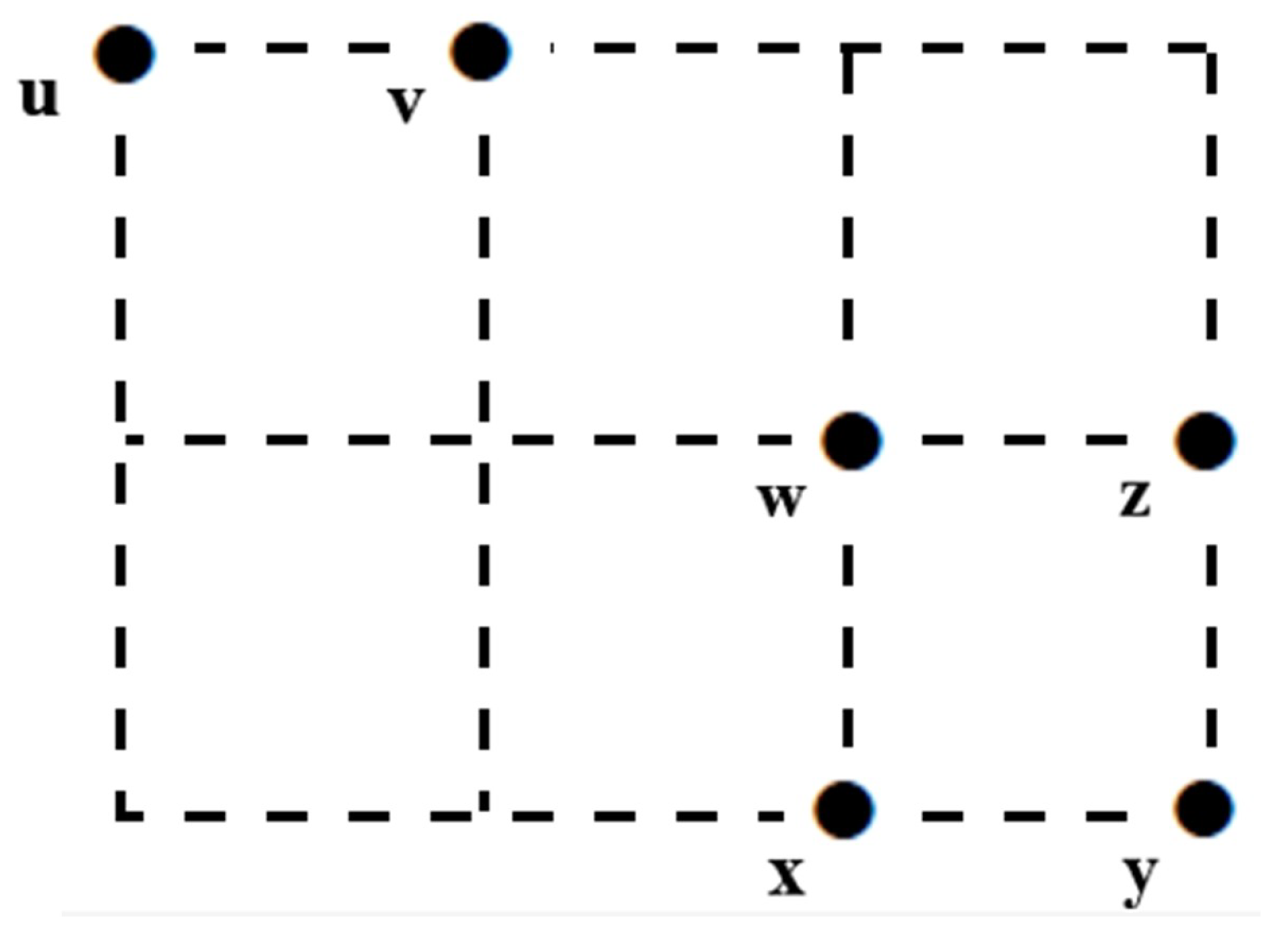
([22]). Let X be an MA-space. The nth singular homology group of X for each $n\ge 0$ is

$$H_n\left(X\right):={\displaystyle \frac{Kernel{\partial }_n}{Image{\partial }_{n+1}}}.$$

For $z_n\in Z_n\left(X\right)$, the coset $z_n+B_n\left(X\right)$ is called the homology class of $z_n$ and is denoted by ${\overline{z}}_n$.

Example 1. 

Let $X=\{u=(-2,2),v=(-1,2),w=(0,1),x=(0,0),y=(1,0),z=(1,1\left)\right\}$ be the MA-space (in Figure 2). We determine the digital homology groups of the MA-space X.

The M-topology on X is induced by the basis $\mathcal{B}=\left\{\right\{v\},\{w\},\{y\},\{u,v\},\{x,y,w\},\{x,y,z\left\}\right\}$ as follows:

$$\begin{array}{cc}\hfill {\gamma }_X=& \{\varnothing ,X,\{v\},\{w\},\{y\},\{u,v\},\{v,w\},\{v,y\},\{w,y\},\{u,v,w\},\{v,w,y\},\{x,y,w\},\hfill \\ & \{x,y,z\},\{u,v,y\},\{v,x,y\},\{u,v,w,y\},\{v,w,x,y\},\{v,x,y,z\},\{w,x,y,z\},\hfill \\ & \{u,v,x,y,z\},\{u,v,w,x,y\},\{v,w,x,y,z\}\}.\hfill \end{array}$$

•

$S_0\left(X\right)\cong {\mathbb{Z}}^6$, since $\{{\sigma }_i^0:e_0\to p:p\in X,i\in {[1,6]}_{\mathbb{Z}}\}$ is a basis for $S_0\left(X\right)$.

•

$S_1\left(X\right)\cong {\mathbb{Z}}^{11}$, since $S_1\left(X\right)$ has the basis $\{{\sigma }_i^1:i\in {[1,11]}_{\mathbb{Z}}\}$, where

$$\begin{array}{cccccccccccc}\hfill {\sigma }_1^1:& e_0\mapsto u\hfill & \hfill {\sigma }_2^1:& e_0\mapsto v\hfill & \hfill {\sigma }_3^1:& e_0\mapsto w\hfill & \hfill {\sigma }_4^1:& e_0\mapsto x\hfill & \hfill {\sigma }_5^3:& e_0\mapsto y\hfill & \hfill {\sigma }_6^3:& e_0\mapsto z\hfill \\ \hfill & e_1\mapsto u\hfill & \hfill & e_1\mapsto v\hfill & \hfill & e_1\mapsto w\hfill & \hfill & e_1\mapsto x\hfill & \hfill & e_1\mapsto y\hfill & \hfill & e_1\mapsto z\hfill \\ \hfill {\sigma }_7^1:& e_0\mapsto u\hfill & \hfill {\sigma }_8^1:& e_0\mapsto x\hfill & \hfill {\sigma }_9^1:& e_0\mapsto x\hfill & \hfill {\sigma }_{10}^1:& e_0\mapsto z\hfill & \hfill {\sigma }_{11}^1:& e_0\mapsto z\hfill \\ \hfill & e_1\mapsto v\hfill & \hfill & e_1\mapsto y\hfill & \hfill & e_1\mapsto w\hfill & \hfill & e_1\mapsto y\hfill & \hfill & e_1\mapsto w\hfill \end{array}$$

•

$S_n\left(X\right)\cong 0$ for $n\ge 2$, by Remark 2.

Hence, we have the following digital singular complex:

$$0\stackrel{{\partial }_2}{\to }{\mathbb{Z}}^{11}\stackrel{{\partial }_1}{\to }{\mathbb{Z}}^6\stackrel{{\partial }_0}{\to }0$$

It is obvious from the sequence above that $Ker{\partial }_0\cong {\mathbb{Z}}^6$ and $Im{\partial }_2\cong 0$.

Consider the differential map ${\partial }_1:S_1\left(X\right)\to S_0\left(X\right)$ defined by

$${\partial }_1\left({\sigma }_i^1\right)={\sigma }_i^1\left(e_1\right)-{\sigma }_i^1\left(e_0\right);\mathrm{for}i\in {[1,11]}_{\mathbb{Z}}.$$

We have

$$\begin{array}{cccc}\hfill & {\partial }_1\left({\sigma }_1^1\right)=0\hfill & \hfill & {\partial }_1\left({\sigma }_7^1\right)=v-u={\sigma }_2^0-{\sigma }_1^0\hfill \\ \hfill & {\partial }_1\left({\sigma }_2^1\right)=0\hfill & \hfill & {\partial }_1\left({\sigma }_8^1\right)=y-x={\sigma }_5^0-{\sigma }_4^0\hfill \\ \hfill & {\partial }_1\left({\sigma }_3^1\right)=0\hfill & \hfill & {\partial }_1\left({\sigma }_9^1\right)=w-x={\sigma }_3^0-{\sigma }_4^0\hfill \\ \hfill & {\partial }_1\left({\sigma }_4^1\right)=0\hfill & \hfill & {\partial }_1\left({\sigma }_{10}^1\right)=y-z={\sigma }_5^0-{\sigma }_6^0\hfill \\ \hfill & {\partial }_1\left({\sigma }_5^1\right)=0\hfill & \hfill & {\partial }_1\left({\sigma }_{11}^1\right)=w-z={\sigma }_3^0-{\sigma }_6^0\hfill \\ \hfill & {\partial }_1\left({\sigma }_6^1\right)=0\hfill & \hfill \end{array}$$

Let ${\displaystyle {\partial }_1\left(\sum _{i=1}^{11}{t}_i{\sigma }_i^1\right)=0}$ where $t_i\in \mathbb{Z}$ and $i\in {[1,11]}_{\mathbb{Z}}$. We can write ${\displaystyle \sum _{i=1}^{11}{t}_i{\partial }_1\left({\sigma }_i^1\right)=0}$ by the linearity of ${\partial }_1$. When we solve the equation

$$-t_7{\sigma }_1^0+t_7{\sigma }_2^0+(t_9+t_{11}){\sigma }_3^0+(-t_8-t_9){\sigma }_4^0+(t_8+t_{10}){\sigma }_5^0+(-t_{10}-t_{11}){\sigma }_6^0=0$$

we obtain $t_8=-t_9=-t_{10}=t_{11}$, so $Ker{\partial }_1\cong {\mathbb{Z}}^7$ and $Im{\partial }_1\cong {\mathbb{Z}}^4$.

Hence, the singular homology groups of the MA-space X are

$$\begin{array}{c}\hfill H_n\left(X\right)=\left\{\begin{array}{cc}{\mathbb{Z}}^2,\hfill & \mathit{if}n=0;\hfill \\ {\mathbb{Z}}^7,\hfill & \mathit{if}n=1;\hfill \\ 0,\hfill & \mathit{if}n\ge 2.\hfill \end{array}\right.\end{array}$$

Characterization 1. 

Consider the MA-space $X=\{a,b,c,d\}$ (see Figure 3) consisting of points either all odd or mixed even and double even.

Since M-topology on X corresponds to discrete topology, every digital singular n-simplex is continuous only when it is constant. Thus, we have $S_n\left(X\right)\cong {\mathbb{Z}}^4$ for $n=0,1$ and $S_n\left(X\right)\cong 0$ for $n\ge 2$.

$$Ker{\partial }_n\left(X\right)=\left\{\begin{array}{cc}{\mathbb{Z}}^4,\hfill & \mathit{if}n=1;\hfill \\ 0,\hfill & \mathit{if}n\ne 1.\hfill \end{array}\right.Im{\partial }_n\left(X\right)=\left\{\begin{array}{cc}{\mathbb{Z}}^4,\hfill & \mathit{if}n\ne 1;\hfill \\ 0,\hfill & \mathit{if}n=1.\hfill \end{array}\right.$$

Consequently $H_0\left(X\right)\cong {\mathbb{Z}}^4$, and $H_n\left(X\right)\cong 0$ for $n\ne 0$.

3. Some Properties of Homology Groups of MA-Spaces

Theorem 2. 

If X is a one-point MA-space, then we have $H_0\left(X\right)\cong \mathbb{Z}$ and $H_n\left(X\right)\cong 0$ for all $n>0$.

Proof. 

For each $n\ge 0$, there is precisely one digital singular n-simplex ${\sigma }^n\in S_n\left(X\right)$ that is the constant map.

$${\partial }_n\left({\sigma }^n\right)=\left\{\begin{array}{cc}0,\hfill & n\mathrm{is}\mathrm{odd};\hfill \\ {\sigma }^{n-1},\hfill & n\mathrm{is}\mathrm{even}\mathrm{and}\mathrm{positive},\hfill \end{array}\right.$$

since ${\displaystyle {\partial }_n\left({\sigma }^n\right)=\sum _{i=0}^n{(-1)}^i{\sigma }^n{\epsilon }_i=\sum _{i=0}^n{\sigma }^{n-1}}$.

In the case where n is odd, ${\partial }_n=0$ and hence $S_n\left(X\right)=Ker{\partial }_n=Z_n\left(X\right)$. ${\partial }_{n+1}$ is an isomorphism (for even $n+1$), which implies $S_n\left(X\right)=Im{\partial }_{n+1}=B_n\left(X\right)$. It follows that $H_n\left(X\right)\cong 0$. If n is positive and even, then ${\partial }_n$ becomes an isomorphism. Since ${\partial }_n=Z_n\left(X\right)=0$, we obtain $H_n\left(X\right)\cong 0$.

When $n=0$, since X is a one-point space, $S_0\left(X\right)=\langle {\sigma }^n\rangle \cong \mathbb{Z}$. Hence, $Z_0\left(X\right)=Ker{\partial }_0\cong \mathbb{Z}$. Also, $Im{\partial }_1=B_0\left(X\right)=0$ ($n=1$ is odd). Thus, $H_0\left(X\right)=Z_0\left(X\right)/B_0\left(X\right)=\mathbb{Z}/0\cong \mathbb{Z}$. □

Let X and Y be two MA-spaces. If $f:X\to Y$ is an MA-map and ${\sigma }^n:{\Delta }^n\to X$ is a singular n-simplex in X, then $f\circ {\sigma }^n:{\Delta }^n\to Y$ is also a singular n-simplex in Y. If f is extended by the linearity of singular n-simplexes in X, we get a homomorphism

$$\begin{gathered} {\displaystyle f_{♯}:S_n\left(X\right)\to S_n\left(Y\right) \\ \sum _{i=1}^n{t}_i{\sigma }_i^n\mapsto f_{♯}\left(\sum _{i=1}^n{t}_i{\sigma }_i^n\right)=\sum _{i=1}^n{t}_i(f\circ {\sigma }_i^n)} \end{gathered}$$

where $t_i\in \mathbb{Z}$.

One can easily prove Theorem 3 and Theorem 4 in a very similar way to [25].

Theorem 3. 

If $f:X\to Y$ is an MA-map where X and Y are two MA-spaces, then $f_{♯}{\partial }_n^X={\partial }_n^Y{f}_{♯}$.

Theorem 4. 

Let X and Y be two MA-spaces, and $f:X\to Y$ is an MA-map. Then, for every $n\ge 0$,

$$f_{♯}\left(Z_n\left(X\right)\right)\subset Z_n\left(Y\right) \mathit{and} f_{♯}\left(B_n\left(X\right)\right)\subset B_n\left(Y\right).$$

The category of M-topological spaces with MA-adjacency (for short MAC) was considered first by Han [24] in order to indicate that MAC is equivalent to DTC(4) (Digital Topological Category).

Theorem 5. 

If X is a path-connected MA-space, then $H_0\left(X\right)\cong \mathbb{Z}$.

Proof. 

Let X be a path-connected MA-space. Since MAC is equivalent to DTC(4), which is the category whose objects are digital images with 4-adjacency in ${\mathbb{Z}}^2$ and morphisms are (digitally) 4-continuous maps [24], one can easily say that X is a 4-connected digital image and hence $H_0\left(X\right)\cong \mathbb{Z}$. □

Remark 3. 

It is well known that $H_n$ is a functor [25]; however, we would like to emphasise here that $H_n:MAC\to Ab$ is the homology functor between the category of MA-spaces (MAC) and the category of abelian groups (Ab) for every $n\ge 0$ where the objects of MAC are MA-spaces and the morphisms are MA-maps.

Theorem 6. 

$H_n:MAC\to Ab$ is a functor for every $n\ge 0$.

Proof. 

Let X and Y be two MA-spaces and $f:X\to Y$ be an MA-map. Define

$$\begin{gathered} H_n:H_n\left(X\right)\to H_n\left(Y\right) \\ \overline{z}=z_n+B_n\left(X\right)\mapsto H_n\left(f\right)\left(\overline{z}\right)=f_{♯}\left(z_n\right)+B_n\left(Y\right) \end{gathered}$$

where $z_n\in Z_n\left(X\right)$. Since $z_n$ is an n-cycle in X, $f_{♯}\left(z_n\right)$ is also an n-cycle in Y. By the independence of the choice of representative, $f_{♯}\left(B_n\left(X\right)\right)\subset B_n\left(Y\right)$.

$H_n$ is a homomorphism, since for all ${\overline{z}}_n,{\overline{z}}_n^{\prime }\in H_n\left(X\right)$

$$\begin{array}{cc}\hfill H_n\left(f\right)({\overline{z}}_n+{\overline{z}}_n^{\prime })=& f_{♯}(z_n+z_n^{\prime })+B_n\left(Y\right)\hfill \\ \hfill =& (f_{♯}\left(z_n\right)+f_{♯}\left(z_n^{\prime }\right))+B_n\left(Y\right)\hfill \\ \hfill =& f_{♯}\left(z_n\right)+B_n\left(Y\right)+f_{♯}\left(z_n^{\prime }\right)+B_n\left(Y\right)\hfill \\ \hfill =& H_n\left(f\right)\left({\overline{z}}_n\right)+H_n\left(f\right)\left({\overline{z}}_n^{\prime }\right).\hfill \end{array}$$

Since for every $X\in Obj\left(MAC\right)$ and $1_X$ identity MA-map $H_n\left(1_X\right)=1_{H_n\left(X\right)}$, $H_n$ preserves identity.

Let X, Y, and W be MA-spaces and let $f:X\to Y$ and $g:Y\to W$ be two MA-maps. Then, $H_n$ preserves the combination as follows:

$$\begin{array}{cc}\hfill H_n(g\circ f)\left({\overline{z}}_n\right)=& {(g\circ f)}_{♯}\left(z_n\right)+B_n\left(W\right)\hfill \\ \hfill =& g_{♯}(f_{♯}\left(z_n\right)+B_n\left(Y\right))\hfill \\ \hfill =& g_{♯}\left(f_{♯}(\left(z_n\right)+B_n\left(X\right))\right)\hfill \\ \hfill =& (H_n\left(g\right)\circ H_n\left(f\right))\left({\overline{z}}_n\right).\hfill \end{array}$$

Thus, $H_n$ is a functor. □

As a consequence of $H_n$ being a functor, we have the following corollary.

Corollary 1. 

If X and Y are MA-isomorphic, then

$$H_n\left(X\right)\cong H_n\left(Y\right)$$

for all $n\ge 0$.

Theorem 7. 

If X is an MA-space and $X_j$ is the set of path-connected components of X, then for every $n\ge 0$,

$${\displaystyle H_n\left(X\right)\cong \underset{j}{⨁}{H}_n\left(X_j\right).}$$

Proof. 

The proof is same as the algebraic topology version. □

4. Relative Homology Groups of MA-Spaces and Excision Theorem

Let X be an MA-space, A be a subspace of X, and $i:A\hookrightarrow X$ be the inclusion map. One can easily show that the homomorphism induced by i is a monomorphism. The quotient group

$$S_n(X,A):=S_n\left(X\right)/S_n\left(A\right)$$

is called the group of relative n-dimensional chains of X modulo A (i.e., n-dimensional chain group of the pair $(X,A)$).

There is a homomorphism ${\partial }_n:S_n\left(X\right)\to S_{n-1}\left(X\right)$, since

$$\begin{array}{cc}\hfill {\partial }_n:S_n\left(X\right)& \to S_{n-1}\left(X\right)\hfill \\ \hfill S_n\left(A\right)& \mapsto {\partial }_n\left(S_n\left(A\right)\right)\subset S_{n-1}\left(A\right),\hfill \end{array}$$

and this homomorphism induces

$${\partial }_n:S_n(X,A)\to S_{n-1}(X,A).$$

${\partial }_n{\partial }_{n+1}=0$, because the induced homomorphism is a boundary operator.

$$Z_n(X,A):=Ker{\partial }_n=\left\{s\in S_n(X,A)|{\partial }_n\left(s\right)=0\right\}$$

is called the group of n-dimensional cycles and

$$B_n(X,A):=Im{\partial }_{n+1}=\left\{{\partial }_{n+1}\left(S_{n+1}(X,A)\right)\right\}$$

is called the group of n-dimensional boundaries for every $n\ge 0$.

The quotient group

$$H_n(X,A)=Z_n(X,A)/B_n(X,A)$$

is called the n-dimensional relative homology groups for the pair $(X,A)$.

If we consider $i:A\hookrightarrow X$ and $j:X\hookrightarrow (X,A)$ as inclusion maps, i and j induce the following homomorphisms, respectively:

$$i_{♯}:S_n\left(A\right)\to S_n\left(X\right)\mathrm{and}{j}_{♯}:S_n\left(X\right)\to S_n(X,A),$$

and

$$i_{*}:H_n\left(A\right)\to H_n\left(X\right)\mathrm{and}{j}_{*}:H_n\left(X\right)\to H_n(X,A).$$

The homomorphism

$$\begin{array}{cc}\hfill d_n:H_n(X,A)& \to H_{n-1}\left(A\right)\hfill \\ \hfill cls{z}_n& \mapsto cls{i}_{n-1}^{-1}{\partial }_n{j}_n^{-1}{z}_n\hfill \end{array}$$

is called the connecting homomorphism of the pair $(X,A)$. There exists an exact sequence of groups and homomorphisms that is called the exact homology sequence of the pair $(X,A)$:

$$\dots \stackrel{j_{*}}{\to }{H}_{n+1}(X,A)\stackrel{{\partial }_{*}}{\to }{H}_n\left(A\right)\stackrel{i_{*}}{\to }{H}_n\left(X\right)\stackrel{{\partial }_{*}}{\to }\dots .$$

Example 2. 

Consider the MA-space that is given in Example 1 and $A=\left\{u,v,w\right\}$ as a subset of X. The M-topology on A is ${\gamma }_A=\left\{\varnothing ,A,\left\{v\right\},\left\{w\right\},\left\{u,v\right\},\left\{v,w\right\}\right\}$.

We should start with determining the homology groups of A.

•

$S_0\left(A\right)\cong {\mathbb{Z}}^3$, since $\{{\sigma }_i^0:e_0\to p:p\in A,i\in {[1,3]}_{\mathbb{Z}}\}$ is a basis for $S_0\left(A\right)$.

•

$S_1\left(A\right)\cong {\mathbb{Z}}^4$, since $S_1\left(A\right)$ has the basis $\{{\sigma }_i^1:i\in {[1,4]}_{\mathbb{Z}}\}$, where

$$\begin{array}{cccccccc}\hfill {\sigma }_1^1:& e_0\mapsto u\hfill & \hfill {\sigma }_2^1:& e_0\mapsto v\hfill & \hfill {\sigma }_3^1:& e_0\mapsto w\hfill & \hfill {\sigma }_4^1:& e_0\mapsto u\hfill \\ \hfill & e_1\mapsto u\hfill & \hfill & e_1\mapsto v\hfill & \hfill & e_1\mapsto w\hfill & \hfill & e_1\mapsto v\hfill \end{array}$$

•

$S_n\left(A\right)\cong 0$ for $n\ge 2$, by Remark 2.

We have the following digital singular complex:

$$0\stackrel{{\partial }_2}{\to }{\mathbb{Z}}^4\stackrel{{\partial }_1}{\to }{\mathbb{Z}}^3\stackrel{{\partial }_0}{\to }0$$

It is evident that $Ker{\partial }_0\cong {\mathbb{Z}}^3$ and $Im{\partial }_2\cong 0$.

For ${\sigma }_i^1\in S_1\left(A\right)$, consider the differential map ${\partial }_1:S_1\left(A\right)\to S_0\left(A\right)$ such that

$${\partial }_1\left({\sigma }_i^1\right)={\sigma }_i^1\left(e_1\right)-{\sigma }_i^1\left(e_0\right);\mathit{for}i\in {[1,4]}_{\mathbb{Z}}.$$

Then,

$$\begin{array}{cc}\hfill {\partial }_1\left({\sigma }_1^1\right)=& 0\hfill \\ \hfill {\partial }_1\left({\sigma }_2^1\right)=& 0\hfill \\ \hfill {\partial }_1\left({\sigma }_3^1\right)=& 0\hfill \\ \hfill {\partial }_1\left({\sigma }_4^1\right)=& {\sigma }_2^0-{\sigma }_1^0\hfill \end{array}$$

Let ${\displaystyle {\partial }_1\left(\sum _{i=1}^4{t}_i{\sigma }_i^1\right)=0}$ where $t_i\in \mathbb{Z}$ and $i\in {[1,4]}_{\mathbb{Z}}$. We can write ${\displaystyle \sum _{i=1}^4{t}_i{\partial }_1\left({\sigma }_i^1\right)=0}$ by the linearity of ${\partial }_1$. When we solve the equation $t_4{\sigma }_1^0-t_4{\sigma }_2^0=0$, we obtain $Ker{\partial }_1\cong {\mathbb{Z}}^3$ and $Im{\partial }_1\cong \mathbb{Z}$.

Thus, the singular homology groups of the MA-space A are

$$\begin{array}{c}\hfill H_n\left(A\right)=\left\{\begin{array}{cc}{\mathbb{Z}}^2,\hfill & \mathit{if}n=0;\hfill \\ {\mathbb{Z}}^3,\hfill & \mathit{if}n=1;\hfill \\ 0,\hfill & \mathit{if}n\ge 2.\hfill \end{array}\right.\end{array}$$

By using the exact sequence for $(X,A)$, we write

$$0\to H_2(X,A)\to {\mathbb{Z}}^3\to {\mathbb{Z}}^7\to H_1(X,A)\to {\mathbb{Z}}^2\to {\mathbb{Z}}^2\to H_0(X,A)\to 0.$$

The results indicate that $H_0(X,A)\cong 0$, $H_1(X,A)\cong {\mathbb{Z}}^4$, and $H_2(X,A)\cong 0$.

Proposition 1. 

Let X be an MA-space and $A\subset X$. If A is empty set, then $H_n(X,A)\cong H_n\left(X\right)$ for all $n\ge 0$.

Proof. 

$H_n\left(A\right)\cong 0$ for all $n\ge 0$, since A is an empty set. By using the exact homology sequence, we have the following short sequence:

$$0\to H_n\left(X\right)\stackrel{p_{*}}{\to }{H}_n(X,A)\to 0.$$

Since $p_{*}$ is an isomorphism, we obtain the required result. □

Proposition 2. 

Let X be an MA-space and $A\subset X$. If $A=\left\{q\right\}$ is the singleton set, then $H_n(X,A)\cong H_n\left(X\right)$ for all $n>0$.

Proof. 

$H_n\left(A\right)\cong 0$ for all $n>0$ from Theorem 2. By using the exact homology sequence, we have the following short sequence:

$$0\to H_n\left(X\right)\stackrel{p_{*}}{\to }{H}_n(X,A)\to 0.$$

Hence, $H_n\left(X\right)\cong H_n(X,A)$, since $p_{*}$ is an isomorphism. □

Proposition 3. 

$H_n(X,X)\cong 0$ for all $n\ge 0$ and any MA-space X.

Proof. 

If we consider the exact homology sequence for the pair $(X,X)$, the inclusion map $i:X\to X$ induces the identity homomorphism $i_{*}:H_n\left(X\right)\to H_n\left(X\right)$. Thus, we obtain the required result. □

Let us take $A_1$ and $A_2$ as the subsets of an MA-space X such that $X=A_1^{\circ }\cup A_2^{\circ }$; also, consider the following diagram where each map is an inclusion map:

$$\begin{array}{c}(A_1\cap A_2,\varnothing )\stackrel{i}{\to }(A_1,\varnothing )\stackrel{p}{\to }(X,A_1\cap A_2)\\ h\downarrow \downarrow g\downarrow j\\ (A_2,\varnothing )\underset{f}{\to }(X,\varnothing )\underset{q}{\to }(X,A_2)\end{array}$$

One can reproduce the Excision Theorem of algebraic topology for appropriate MA-spaces [25].

Theorem 8. 

(Excision) Let X be an MA-space; $A_1$ and $A_2$ are subsets of X such that and $X=A_1^{\circ }\cup A_2^{\circ }$. Then, the inclusion $j:(A_1,A_1\cap A_2)\hookrightarrow (X,A_2)$ induces the following isomorphisms for all n:

$$j_{*}:H_n(A_1,A_1\cap A_2)\to H_n(X,A_2).$$

The Excision Theorem in the digital setting plays a key role in extending local homological information to global structures, which is crucial in image analysis. Unlike the classical case, where excision depends on open sets, the digital approach must work within adjacency-based, discrete environments—making this adaptation both nontrivial and practically significant.

Example 3. 

Consider the MA-space $X=\{u=(-2,2),v=(-1,2),w=(0,1),x=(0,0),y=(1,0),z=(1,1\left)\right\}$ given in Example 1, and take $A_1=\{u,v,w\}$ and $A_2=\{w,x,y,z\}$. For $A_1$ and $A_2$, the hypothesis of Excision holds; that is, $A_1,A_2\in {\gamma }_X$ and $A_1\cup A_2=X$. By using the Excision Theorem, we have the following isomorphisms for all $n\ge 0$:

$$H_n(\{u,v,w\},\left\{w\right\})\cong H_n(X,\{w,x,y,z\}).$$

Also, by using Proposition 2, we have the following homology groups of the pair $\left(\right\{u,v,w\},\{w\left\}\right)$:

$$H_0(A_1,A_1\cap A_2)\cong {\mathbb{Z}}^2{H}_1(A_1,A_1\cap A_2)\cong {\mathbb{Z}}^3{H}_n(A_1,A_1\cap A_2)\cong 0,\mathit{for}\forall n\ge 2.$$

5. Conclusions

This study established the functoriality of digital singular homology on MA-spaces by formulating a homology functor from the category of MA-spaces (MAC) to the category of abelian groups (Ab). In addition, several foundational properties of homology groups associated with MA-spaces were examined. A significant contribution of this work is the introduction of digital relative homology groups within the context of Marcus–Wyse topology, along with a demonstration that the excision property holds for spaces in the MAC category.

The results presented here aim to support the computation of homology groups on localized regions of digital images, provided the global homological structure is known. This opens pathways for more efficient analysis of complex digital images through modular and topologically informed approaches. While the techniques employed parallel those used in frameworks based on the category of digital topological spaces (DTC) and category of Khalimsky digital topological spaces (KDTC), the results obtained here reflect structural distinctions unique to the Marcus–Wyse topology. One can see that because of its symmetry and minimal neighborhood variation, algorithms that use Marcus–Wyse topology can be faster to compute, with fewer edge conditions than those using Khalimsky’s model.

These findings are especially relevant in applications where high-resolution digital image analysis demands both topological accuracy and computational efficiency—for example, in medical imaging, shape recognition, and 3D object reconstruction. By introducing relative homology structures that remain stable under adjacency relations induced by the Marcus–Wyse topology, this study offers a new algebraic framework that aligns more closely with the inherently discrete nature of digital images than traditional models. As such, the proposed approach not only addresses existing theoretical gaps but also provides a foundation for future developments in topological image analysis.

Future research building upon this work will focus on the development of digital singular cohomology theories for digital spaces endowed with Khalimsky and Marcus–Wyse topologies, and their comparison with corresponding digital simplicial cohomology theory. This comparative study is expected to further clarify the algebraic and topological nuances among digital cohomological frameworks and their suitability for various applications in digital image analysis.