Statistical Inference and Goodness-of-Fit Assessment Using the AAP-X Probability Framework with Symmetric and Asymmetric Properties: Applications to Medical and Reliability Data

Abstract

Probability models are instrumental in a wide range of applications by being able to accurately model real-world data. Over time, numerous probability models have been developed and applied in practical scenarios. This study introduces the AAP-X family of distributions—a novel, flexible framework for continuous data analysis named after authors Aadil Ajaz and Parvaiz. The proposed family effectively accommodates both symmetric and asymmetric characteristics through its shape-controlling parameter, an essential feature for capturing diverse data patterns. A specific subclass of this family, termed the “AAP Exponential” (AAPEx) model is designed to address the inflexibility of classical exponential distributions by accommodating versatile hazard rate patterns, including increasing, decreasing and bathtub-shaped patterns. Several fundamental mathematical characteristics of the introduced family are derived. The model parameters are estimated using six frequentist estimation approaches, including maximum likelihood, Cramer–von Mises, maximum product of spacing, ordinary least squares, weighted least squares and Anderson–Darling estimation. Monte Carlo simulations demonstrate the finite-sample performance of these estimators, revealing that maximum likelihood estimation and maximum product of spacing estimation exhibit superior accuracy, with bias and mean squared error decreasing systematically as the sample sizes increases. The practical utility and symmetric–asymmetric adaptability of the AAPEx model are validated through five real-world applications, with special emphasis on cancer survival times, COVID-19 mortality rates and reliability data. The findings indicate that the AAPEx model outperforms established competitors based on goodness-of-fit metrics such as the Akaike Information Criteria (AIC), Schwartz Information Criteria (SIC), Akaike Information Criteria Corrected (AICC), Hannan–Quinn Information Criteria (HQIC), Anderson–Darling (A*) test statistic, Cramer–von Mises (W*) test statistic and the Kolmogorov–Smirnov (KS) test statistic and its associated p-value. These results highlight the relevance of symmetry in real-life data modeling and establish the AAPEx family as a powerful tool for analyzing complex data structures in public health, engineering and epidemiology.

1. Introduction

Probability models play a crucial role in statistical analysis, data modeling and real-world applications. However, no single probabilistic model can consistently outperform all others across diverse datasets and scenarios. This inherent limitation fuels ongoing research, inspiring statisticians to craft new probability distributions tailored to specific needs. Modifying or extending existing models often yields distributions that fit real-world data more closely than their predecessors. This drive for better fit, greater flexibility and wider applicability spans multiple disciplines and motivates continuous innovation.

One of the earliest and most fundamental methods for generating new distributions was introduced by Mudholkar and Srivastava [1], who crafted the Exponentiated Family of Distributions. Their elegant approach enhances a baseline distribution by adding a shape parameter—a simple twist that unlocks a broader spectrum of data patterns. It is an undeniable truth that no model reigns supreme; hence, statisticians tirelessly explore fresh models to capture reality’s complexities. The cumulative distribution function (CDF) of the exponentiated family is given by

$$F(x;\gamma ,\zeta )={\left[G(x;\zeta )\right]}^{\gamma },\gamma ,\zeta >0,x\in \mathbb{R}.$$

(1)

Here, $\gamma$ adds a new dimension of shape and $G(x;\zeta )$ is the CDF of the base distribution, itself defined by $\zeta$ parameters. This elegant formulation breathes flexibility into classical distributions, molding them to suit intricate datasets.

Following this, Reference [2] introduced the Marshall–Olkin family of distributions. Their transformation reshapes the baseline CDF with an $\alpha$ parameter, yielding the following:

$${\overline{F}}_{MO}(\alpha ;x)={\displaystyle \frac{\alpha \overline{F}\left(x\right)}{1-\overline{\alpha }\overline{F}\left(x\right)}};\alpha >0,\overline{\alpha }=1-\alpha ,x\in \mathbb{R},$$

(2)

where $\overline{F}\left(x\right)=1-F\left(x\right)$ represents the survival function. This structure grants finer control over tail behavior, making it invaluable for reliability and risk analysis.

Building on this foundation, Reference [3] proposed the Alpha Power Transformation (APT), introducing a parameter ($\alpha$) that redefines the baseline CDF ($G(x;\beta )$) as follows:

$$F(x;\alpha ,\zeta )=\left\{\begin{array}{cc}{\displaystyle \frac{{\alpha }^{G(x;\zeta )}-1}{\alpha -1}},\hfill & \alpha >0,\alpha \ne 1\hfill \\ G(x;\beta ),\hfill & \alpha =1\hfill \end{array}\right..$$

(3)

This transformation injects fresh flexibility, with the exponential distribution appearing as a special, illuminating case.

To further expand the toolkit, Reference [4] introduced the MIT transformation—named after its creators, Murtaza, Ishfaq and Tariq—enhancing a baseline CDF by weaving in a shape parameter ($\alpha$):

$$F_{MIT}(x;\alpha )={\displaystyle \frac{\alpha F\left(x\right)}{1-\overline{\alpha }F\left(x\right)}};\alpha >0,\overline{\alpha }=1-\alpha ,x\in \mathbb{R}.$$

(4)

This simple yet powerful tweak opens doors to greater modeling flexibility.

Expanding horizons, Reference [5] applied the T-X family methodology by Reference [6] to create the New Exponent Power-X (NGEP-X) family, whose CDF reads as follows:

$$F(x;\alpha ,\zeta )=1-\left(e^{\alpha G(x;\zeta )}-e^{\alpha }G(x;\zeta )\right),\alpha >0,x\in \mathbb{R}.$$

(5)

This formulation melds exponential power with a new perspective, enriching distribution shapes.

Meanwhile, Reference [7] unveiled the alpha-log-power transformed family (ALPTG), embedding a novel shape parameter independent of the parent model, offering fresh avenues for continuous distribution modeling:

$$F_{ALPTG}\left(x\right)={\alpha }^{log\left({\displaystyle \frac{1}{G(x;\gamma )}}\right)},$$

(6)

Continuing the innovation, Reference [8] proposed the New Logarithmic Tangent-U (NLT-U) family, introducing the NLT-Wei model, a flexible Weibull-based sub-model. It showcases hazard functions that curve and twist—rising, falling, unimodal and bathtub-shaped functions—capturing real-world failure behaviors.

Riding the wave of novel approaches, Reference [9] embraced trigonometric transformations, crafting a family where the baseline distribution undergoes a sine- and cosine-inspired metamorphosis:

$$F(x;\zeta )={\displaystyle \frac{e^{1-cos\left(\frac{\pi G(x;\zeta )}{1+G(x;\zeta )}\right)}-1}{e-1}},\zeta >0,x\in \mathbb{R}.$$

(7)

This infusion of trigonometry injects rhythm into the shape of distributions, enhancing their expressive power.

Further enriching this path, Reference [10] introduced the ASP family, a sine-based flexible distribution that masterfully handles skewed and heavy-tailed data:

$$F_{\mathrm{ASP}}(x;\alpha ,\zeta )=2sin\left[{\displaystyle \frac{\pi }{2}}{\left(C(x;\zeta )\right)}^{\alpha }\right]-{\left(C(x;\zeta )\right)}^{\alpha },\alpha ,\zeta >0,x\in \mathbb{R}.$$

(8)

This approach offers a robust alternative for engineering, medicine and beyond.

Finally, Reference [11] proposed the Alpha Beta Power-E (ABPE) Transformation, whose CDF is expressed as follows:

$$G\left(z\right)={\displaystyle \frac{{\alpha }^{F\left(z\right)}-{\beta }^{F\left(z\right)}}{\alpha -\beta }},z\in \mathbb{R},\alpha ,\beta >0,\alpha \ne \beta \ne 1,$$

(9)

bringing yet another harmonious blend of parameters to the family of flexible distributions.

In light of the extensive developments in probability distribution generation techniques discussed above, our study aims to contribute to this ongoing evolution by introducing a novel and more adaptable probability model. Many existing methods enhance baseline distributions by incorporating additional parameters, but these modifications can sometimes lead to re-parameterization issues, increased model complexity and challenges in practical implementation. To address these concerns, we propose an innovative AAP family of distributions, a flexible framework that refines existing distributions while minimizing the complexities associated with parameter inflation. The AAP-X family is designed to enhance the fitting ability of probability distributions, providing a more efficient and adaptable modeling approach. Unlike conventional transformation techniques that merely add parameters, the AAP-X method strategically modifies the structural properties of the base distribution to achieve greater flexibility without excessive parameterization. This innovative framework can effectively capture both symmetric and asymmetric data patterns through its shape-controlling mechanism, making it applicable across diverse domains.

As a specific application of our framework, we introduce an improved version of the exponential distribution using the AAP-X transformation. This enhanced model demonstrates superior flexibility, particularly in terms of its probability density function (PDF) and hazard rate function (HRF), allowing for a more accurate representation of real-life data. To validate its practical relevance and establish its superiority over classical models, we conducted a comparative analysis against several well-known models, including the Alpha Power Exponential and Marshall–Olkin Exponential models. These comparisons, presented in the application section of the manuscript, reveal that the AAP-X family consistently outperforms these traditional models based on standard goodness-of-fit criteria such as the AIC, BIC, AICC, HQIC and KS statistics.

Overall, this study not only introduces a novel statistical transformation but also preserves the theoretical elegance while addressing practical challenges. Its ability to capture diverse data behaviors, particularly symmetry and asymmetry, makes it highly relevant for applications in reliability analysis, survival studies, epidemiology and beyond.

The remainder of this paper is structured as follows: Section 2 presents the research gap and highlights the need for developing the proposed AAP-X family of distributions. Section 3 introduces the proposed AAP-X family of distributions, along with its mathematical formulation and key properties. Section 4 presents a special case of the family based on the exponential distribution, which serves as a tractable and insightful example. It also discusses various structural characteristics of the model, including the hazard rate function, moments and the moment-generating function. In Section 5, estimation of parameters is addressed using six methods of estimation. Section 6 includes a detailed simulation study to compare the performance of estimators. In Section 7, the practical utility of the model is demonstrated through real-world data applications. Finally, Section 8 concludes the paper with a summary of findings and directions for future research.

2. Research Gap

The existing literature on extended distributions, particularly those enhancing baseline models such as the exponential distribution, reveals several limitations and gaps that warrant further investigation. This paper aims to address the following specific research gaps:

• Existing transformation techniques often increase model complexity through additional parameters, leading to parameter inflation without substantial gains in flexibility.
• Several extended models fail to offer adequate flexibility in capturing both symmetric and asymmetric data patterns observed in real-world datasets.
• There has been limited exploration of transformation frameworks that preserve theoretical tractability while enhancing distributional shapes.
• Many proposed models do not comprehensively evaluate estimation techniques, resulting in limited insights into their practical implementation.
• Prior works do not offer extensive empirical comparisons across diverse real-life datasets, especially from both medical and engineering domains.
• Limited research exists to assess the performance of new distributions using a wide range of goodness-of-fit criteria and graphical diagnostics.
• The integration of domain-specific datasets for validation of new models remains underexplored, especially in the context of survival and reliability data.

This study responds to the above research gaps by proposing the AAP-X family of distributions, which enhances model flexibility without excessive parameterization and is validated using extensive real-world applications and simulation-based performance comparisons.

3. The Model and Properties

In this section, we introduce a novel family of probability distributions, termed the Aadil Ajaz–Parvaiz-X (AAP-X) Family. The primary motivation behind the development of this family is to enhance the flexibility of existing probability models by incorporating an additional parameter that adjusts the shape and scale properties of the baseline distribution. This transformation aims to provide better modeling capabilities for complex real-world data structures across various disciplines, including engineering, finance and survival analysis. The AAP-X family is defined by modifying the cumulative distribution function (CDF) of a baseline distribution ($G(x;\zeta )$, where $\zeta$ represents the parameter vector of the base distribution). The transformation introduces a new shape control parameter ($\alpha$) that governs the behavior of the tail and the adaptability of the resulting distribution. To understand the behavior and practical utility of the AAP-X family, we explore key statistical properties.

Definition 1. 

Let $G(x;\zeta )$ represent the CDF of the reference model. Then, the CDF ($F(x;\gamma ,\zeta )$) of the AAP-X family, incorporating the additional shape parameter (γ), is obtained as follows:

$$F(x;\gamma ,\zeta )={\displaystyle \frac{\alpha {\left[G(x;\zeta )\right]}^{\gamma }}{1-\overline{\alpha }{\left[G(x;\zeta )\right]}^{\gamma }}};\alpha ,\gamma ,\zeta ,\in {\mathbb{R}}^{+},x\in \mathcal{R},\overline{\alpha }=1-\alpha .$$

(10)

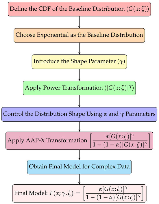
To aid in the understanding of the transformation process from the baseline distribution to the proposed AAP-X family, a schematic flow diagram is presented in Figure 1. This flowchart visually summarizes the key steps involved in deriving the cumulative distribution function (CDF) of the AAP-X family.

Figure 1. Flowchart of the study.

It is straightforward to verify that the cumulative distribution function (CDF) defined in Equation (10) satisfies the essential properties of a valid distribution function. Specifically, the following holds:

$$\underset{x\to -\infty }{lim}F(x;\gamma ,\zeta )=0\mathrm{and}\underset{x\to \infty }{lim}F(x;\gamma ,\zeta )=1,$$

and the function is right-continuous and differentiable. Hence, the expression in Equation (10) is a valid CDF. The probability density function (PDF) corresponding to the CDF in Equation (10) is given by Equation (11):

$$f(x;\gamma ,\zeta )={\displaystyle \frac{\alpha \gamma g(x;\zeta ){\left[G(x;\zeta )\right]}^{\gamma -1}}{{\left[1-\overline{\alpha }{\left[G(x;\zeta )\right]}^{\gamma }\right]}^2}},\alpha ,\gamma ,\zeta \in {\mathbb{R}}^{+},x\in \mathcal{R},\overline{\alpha }=1-\alpha .$$

(11)

Here, $g(x;\zeta )={\displaystyle \frac{d}{dx}}G(x;\zeta )$ is the PDF of the baseline distribution, and $G(x;\zeta )$ is its CDF.

Mathematically, the AAP-X family generalizes several well-established transformation techniques. Its flexibility is illustrated through the following special cases:

• When $\gamma =1$, Equation (10) reduces to Equation (4), representing the MIT technique proposed in Reference [4].
• When $\alpha =1$, Equation (10) simplifies to Equation (1), which corresponds to the exponentiated transformation technique proposed in Reference [1].
• When $\gamma =1$ and $\alpha =1$, Equation (10) collapses to $F\left(x\right)$, the CDF of the baseline distribution.

These reductions confirm that the proposed AAP technique not only generalizes existing transformation approaches but also unifies them under a common framework. Such unification enables a comprehensive exploration of the effects of transformation parameters on the distributional shape, skewness and tail behavior.

3.1. Aging Properties

The term “aging properties” in statistical modeling and survival analysis refers to features of a survival distribution that characterize the evolution of the probability of failure or death. These properties are important in understanding the lifetime behavior and dependability of systems or individuals. For the proposed AAP-X family, the survival function (SF), hazard rate (HR) and cumulative hazard function (CHF) measures are calculated as follows:

$$S(x;\zeta )={\displaystyle \frac{1-{\left[G(x;\zeta )\right]}^{\gamma }}{1-\overline{\alpha }{\left[G(x;\zeta )\right]}^{\gamma }}}.$$

(12)

$$h(x;\zeta )={\displaystyle \frac{\alpha \gamma g(x;\zeta ){\left[G(x;\zeta )\right]}^{\gamma -1}}{\left[1-\overline{\alpha }{\left[G(x;\zeta )\right]}^{\gamma }\right)]\left[1-{\left[G(x;\zeta )\right]}^{\gamma }\right]}}.$$

(13)

$$H(x;\zeta )=-ln\left({\displaystyle \frac{1-{\left[G(x;\zeta )\right]}^{\gamma }}{1-\overline{\alpha }{\left[G(x;\zeta )\right]}^{\gamma }}}\right).$$

(14)

3.2. Quantile Function

The quantile function is an important tool in many statistical methods, including Monte Carlo techniques. By inverting the CDF of a distribution, it is possible to extract random numbers from that distribution. Given a random variable (X) that belongs to the AAP-X family, the quantile function for X can be found in the manner described below:

$$F(x;\zeta )={\displaystyle \frac{\alpha {\left[G(x;\zeta )\right]}^{\gamma }}{1-\overline{\alpha }{G(x;\zeta )]}^{\gamma }}}=u;0<u<1.$$

(15)

Solving for $G(x;\zeta )$, we obtain

$$G(x;\zeta )={\left({\displaystyle \frac{u}{\alpha +\overline{\alpha }u}}\right)}^{{\displaystyle \frac{1}{\gamma }}}$$

(16)

In order to determine the quantile function ($Q_X\left(u\right)$) for the AAP-X family, we need the inversion function of $G(x;\zeta )$. Thus,

$$Q_X\left(u\right)=G^{-1}{\left({\displaystyle \frac{u}{\alpha +\overline{\alpha }u}}\right)}^{{\displaystyle \frac{1}{\gamma }}}$$

(17)

Therefore, by applying Equation (17) for a specific baseline CDF-G, random variates from the AAP family can be generated.

3.3. Moments and Moment-Generating Function

For the AAP-X family introduced in this study, the ordinary rth moment is calculated as

$${{\mu }_r}^{\prime }={\int }_{\Omega }{x}^{r}f(x;\gamma ,\zeta )dx={\int }_{\Omega }{x}^r{\displaystyle \frac{\alpha \gamma g(x;\zeta ){\left[G(x;\zeta )\right]}^{\gamma -1}}{{\left[1-\overline{\alpha }{\left[G(x;\zeta )\right]}^{\gamma }\right]}^2}}dx.$$

(18)

using the following series representation:

$$\begin{array}{c}\hfill {(1-x)}^{-2}=\sum _{a=0}^{\infty }(a+1)x^a;\left|u\right|<1,\end{array}$$

(19)

$$\begin{array}{cc}\hfill {{\mu }_r}^{\prime }& =\alpha \gamma \sum _{k=0}^{\infty }(k+1){\overline{\alpha }}^k{\int }_{\Omega }{x}^r{\left[G(x;\zeta )\right]}^{\gamma (k+1)-1}g(x;\zeta )dx,\hfill \\ & =\alpha \gamma \sum _{k=0}^{\infty }(k+1){\overline{\alpha }}^k{\lambda }_{1,i}(x;\zeta ).\hfill \end{array}$$

where

$${\lambda }_{1,i}(x;\zeta )={\int }_{\Omega }{x}^r{\left[G(x;\zeta )\right]}^{\gamma (k+1)-1}g(x;\zeta )dx.$$

Moreover, the MGF, denoted as $M_x\left(t\right)$ for an AAP-X distributed random variable (X), is obtained as follows:

$$\begin{array}{cc}\hfill M_x\left(t\right)& ={\int }_{\Omega }{\displaystyle \frac{{\left(tx\right)}^r}{r!}}f(x;\gamma ,\zeta )dx,\hfill \\ & =\alpha \gamma \sum _{r,k=0}^{\infty }{\displaystyle \frac{t^r}{r!}}(k+1){\overline{\alpha }}^k{\lambda }_{1,i}(x;\zeta ).\hfill \end{array}$$

3.4. Order Statistics

In distribution theory, order statistics (OS) are essential because they characterize the operational time of systems, and components and are crucial to reliability analysis, estimate theory and life testing. Consider a random sample of observations ($X_1,X_2,X_3,\dots ,X_n$) drawn from the AAP-X family with a CDF and PDF provided by Equations (10) and (11). The PDF of the rth order statistics—say, $X_{r:n}$—is then calculated as follows:

$$f_{r:n}(x;\gamma ,\zeta )={\displaystyle \frac{1}{B(r,n-r+1)}}f(x;\gamma ,\zeta ){\left[F(x;\gamma ,\zeta )\right]}^{r-1}{\left[1-F(x;\gamma ,\zeta )\right]}^{n-r},$$

(20)

The expansion of ${\left[1-F(x;\gamma ,\zeta )\right]}^{n-r}$ in binomial form is provided as follows:

$${\left[1-F(x;\gamma ,\zeta )\right]}^{n-r}=\sum _{k=0}^{n-r}\left({\displaystyle \genfrac{}{}{0pt}{}{n-r}{k}}\right){(-1)}^k{\left[F(x;\gamma ,\zeta )\right]}^k,$$

(21)

By substituting Equation (21) in Equation (20), we derive

$$f_{r:n}(x;\alpha ,\zeta )={\displaystyle \frac{1}{B(r,n-r+1)}}f(x;\alpha ,\zeta )\sum _{k=0}^{n-r}\left({\displaystyle \genfrac{}{}{0pt}{}{n-r}{k}}\right){(-1)}^k{\left[F(x;\alpha ,\zeta )\right]}^{r+k-1}.$$

(22)

Replacing Equations (10) and (11) in Equation (22) yields the PDF of the $X_{r:n}$ statistics.

3.5. Residual and Reverse Residual Lifetime

The notions of residual lifetime (RL) and reverse residual lifetime (RRL) are widely applicable in several fields, including survival modeling, actuarial science, biometrics and risk assessment. Within the framework of the AAP-X family, the RL of a random variable (X), represented as $R_X\left(t\right)$, is described as follows:

$$\begin{array}{cc}\hfill R_X\left(t\right)& ={\displaystyle \frac{S(x+t)}{S\left(t\right)}},\hfill \\ & ={\displaystyle \frac{(1-{\left[G(x+t;\zeta )\right]}^{\gamma })(1-\overline{\alpha }{\left[G(t;\zeta )\right]}^{\gamma })}{(1-{\left[G(t;\zeta )\right]}^{\gamma })(1-\overline{\alpha }{\left[G(x+t;\zeta )\right]}^{\gamma })}}.\hfill \end{array}$$

In addition, we also derive the expression for the RRL of a random variable (X) following the AAP-X family. The calculated expression denoted as $\overline{R_X}\left(t\right)$ is defined as

$$\begin{array}{cc}\hfill \overline{R_X}\left(t\right)& ={\displaystyle \frac{S(x-t)}{S\left(t\right)}},\hfill \\ & ={\displaystyle \frac{(1-{\left[G(x-t;\zeta )\right]}^{\gamma })(1-\overline{\alpha }{\left[G(t;\zeta )\right]}^{\gamma })}{(1-{\left[G(t;\zeta )\right]}^{\gamma })(1-\overline{\alpha }{\left[G(x-t;\zeta )\right]}^{\gamma })}}.\hfill \end{array}$$

4. Special Case

In this part, we present a specific case within the AAP-X family by extending the exponential distribution.

4.1. AAP Exponential (AAPEx) Distribution

In this subsection of the article, a particular subclass of the AAP-X family, characterized by three parameters is introduced. We refer to this particular model as the AAP Exponential (AAPEx) model. The CDF ($G(x;\eta )$) and PDF ($g(x;\eta )$) of the exponential distribution are defined as follows:

$$G(x;\eta )=1-e^{-\eta x};x\ge 0,\eta >0,$$

(23)

and

$$g(x;\eta )=\eta e^{-\eta x}.$$

(24)

By inserting Equations (23) and (24) into Equations (10) and (11), we get the updated version of the exponential distribution (i.e., AAPEx) model as expressed by

$$F(x;\alpha ,\gamma ,\eta )={\displaystyle \frac{\alpha {(1-e^{-\eta x})}^{\gamma }}{1-\overline{\alpha }{(1-e^{-\eta x})}^{\gamma }}};\alpha ,\gamma ,\eta >0,x>0,\overline{\alpha }=1-\alpha ,$$

(25)

and the PDF takes the form as

$$f(x;\alpha ,\gamma ,\eta )={\displaystyle \frac{\alpha \gamma \eta e^{-\eta x}{(1-e^{-\eta x})}^{\gamma -1}}{{[1-\overline{\alpha }{(1-e^{-\eta x})}^{\gamma }]}^2}}.$$

(26)

In order to enhance reader understanding, we provide the following clear explanations for the roles of each parameter in the proposed AAPEx model:

• The shape and tail behaviors are largely controlled by the $\alpha$ parameter. It improves the flexibility of the model by modifying the weight of the modified function.
• The steepness of the cumulative distribution function is influenced by the $\gamma$ parameter. It influences the skewness and kurtosis, making the model capable of capturing asymmetric patterns in data.
• The $\eta$ parameter is the scale parameter from the baseline exponential distribution. It affects the spread of distribution by controlling the rate of decay.
• For the transformation to stay valid and the resultant function to remain a suitable CDF, the formula expressed as $\overline{\alpha }=1-\alpha$ is utilized.

The statistical properties, including SF ($S(x;\alpha ,\gamma ,\eta )$), HF ($h(x;\alpha ,\gamma ,\eta )$) and CHF ($H(x;\alpha ,\gamma ,\eta )$) for the special sub-model, are derived as follows:

$$S(x;\alpha ,\gamma ,\eta )={\displaystyle \frac{1-{(1-e^{-\eta x})}^{\gamma }}{1-\overline{\alpha }{(1-e^{-\eta x})}^{\gamma }}}.$$

(27)

$$h(x;\alpha ,\gamma ,\eta )={\displaystyle \frac{\alpha \gamma \eta e^{-\eta x}{\left(1-e^{-\eta x}\right)}^{\gamma -1}}{\left[1-\overline{\alpha }{\left(1-e^{-\eta x}\right)}^{\gamma }\right]\left[1-{\left(1-e^{-\eta x}\right)}^{\gamma }\right]}}.$$

(28)

and

$$H(x;\alpha ,\gamma ,\eta )=-ln\left({\displaystyle \frac{1-{(1-e^{-\eta x})}^{\gamma }}{1-\overline{\alpha }{(1-e^{-\eta x})}^{\gamma }}}\right).$$

(29)

In addition, for the QF of X, the AAPEx model is expressed as follows:

$$X_u=ln{\left(1-{\left({\displaystyle \frac{u}{\alpha +\overline{\alpha }u}}\right)}^{{\displaystyle \frac{1}{\gamma }}}\right)}^{{\displaystyle \frac{-1}{\eta }}};0<u<1.$$

(30)

Specifically, $u=0.5,0.25\mathrm{and}0.75$ are used in Equation (30) to determine the quartiles, Bowley’s skewness and Moor’skurtosis of the AAPEx model, respectively (see Table 1).

Table 1. Quantiles, Bowley skewness and Moor’s kurtosis for the AAPEx model under varying parameters.

$\mathit{\lambda }$	$\mathit{\eta }$	$\mathit{\alpha }=0.25$					$\mathit{\alpha }=0.75$
		${\mathit{Q}}_{\mathbf{1}}$	${\mathit{Q}}_{\mathbf{2}}$	${\mathit{Q}}_{\mathbf{3}}$	$\mathit{BSK}$	$\mathit{MKUR}$	${\mathit{Q}}_{\mathbf{1}}$	${\mathit{Q}}_{\mathbf{2}}$	${\mathit{Q}}_{\mathbf{3}}$	$\mathit{BSK}$	$\mathit{MKUR}$
0.25	1.2	0.0939	0.4391	1.0789	0.2991	0.7759	0.0075	0.0939	0.4391	0.5994	1.5439
	1.7	0.0663	0.3100	0.7616			0.0053	0.0663	0.3100
	2.1	0.0537	0.2509	0.6165			0.0043	0.0537	0.2509
	2.5	0.0451	0.2108	0.5179			0.0036	0.0451	0.2108
1.25	1.2	0.8493	1.5092	2.3168	0.1007	0.2929	0.4112	0.8493	1.5092	0.2020	0.5413
	1.7	0.5995	1.0653	1.6354			0.2903	0.5995	1.0653
	2.1	0.4853	0.8624	1.3239			0.2350	0.4853	0.8624
	2.5	0.4077	0.7244	1.1121			0.1974	0.4077	0.7244
2.25	1.2	1.2610	1.9667	2.7949	0.0799	0.2351	0.7476	1.2610	1.9667	0.1577	0.4276
	1.7	0.8901	1.3883	1.9729			0.5277	0.8901	1.3883
	2.1	0.7206	1.1238	1.5971			0.4272	0.7206	1.1238
	2.5	0.6053	0.9440	1.3415			0.3588	0.6053	0.9440

Figure 2 illustrates the PDF curves of the AAPEx model for different settings of the $\alpha$, $\gamma$ and $\eta$ parameters. The plots demonstrate a wide variety of shapes, such as unimodal right-skewed (for $\alpha =0.25$, $\gamma =1.5$ and $\eta =3.75$), J-shaped or strictly increasing (for $\alpha =0.7$, $\gamma =6.5$ and $\eta =0.05$), and L-shaped or right-skewed (for $\alpha =1.5$, $\gamma =1.5$ and $\eta =2.5$). Additionally, a bimodal and asymmetrical shape is observed when $\alpha =0.15$, $\gamma =0.8$ and $\eta =1.5$, while a left-skewed unimodal form arises for $\alpha =0.4$, $\gamma =2.5$ and $\eta =3$. A monotonically decreasing or exponential-type decay is evident for $\alpha =0.9$, $\gamma =1$ and $\eta =3$. These variations highlight the flexibility of the AAPEx model in representing both symmetric and asymmetric distributions, making it a suitable choice for modeling real-world lifetime data.

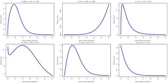
Figure 2. PDF curves of the AAPEx model for different parameter settings of $\alpha$, $\gamma$ and $\eta$.

Figure 3 illustrates the hazard rate function (hrf) of the AAPEx model for various combinations of the $\alpha$, $\gamma$ and $\eta$ parameters and demonstrates its ability to exhibit a wide range of asymmetrical forms. The plots reveal a rich variety of shapes. An increasing hazard rate is observed for $(\alpha =0.7,\gamma =6.5,\eta =0.05)$, while a bathtub-shaped curve appears for $(\alpha =0.15,\gamma =0.5,\eta =2.5)$. An upside-down bathtub shape is evident in the case of $(\alpha =0.15,\gamma =0.3,\eta =2.9)$, and a decreasing hazard rate is shown for $(\alpha =1.5,\gamma =1.5,\eta =0.9)$. Additionally, a reversed J-shaped hrfis observed for $(\alpha =0.9,\gamma =1,\eta =3)$. These distinct forms highlight the flexibility of the AAPED model in capturing various lifetime behaviors and support its applicability to a broad spectrum of real-world reliability data.

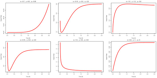
Figure 3. Diverse hazard-rate shapes of the AAPEx model for different settings of $\alpha$, $\gamma$ and $\eta$.

4.2. Moments and Moment-Generating Function

The $r\mathrm{th}$ moment can be calculated by substituting Equations (25) and (26) into Equation (18), which yields

$$\begin{array}{cc}\hfill {{\mu }_r}^{\prime }& =\alpha \eta \gamma \sum _{k=0}^{\infty }(k+1){\overline{\alpha }}^k{\int }_0^{\infty }{x}^r{\left[1-e^{-\eta x}\right]}^{\gamma (k+1)-1}{e}^{-\eta x}dx.\hfill \end{array}$$

(31)

Using series expansion, we obtain the following:

$$\begin{array}{c}\hfill {(1-x)}^n=\sum _{p=0}^{\infty }{(-1)}^p\left({\displaystyle \genfrac{}{}{0pt}{}{n}{p}}\right)x^p\end{array}$$

(32)

$$\begin{array}{cc}\hfill {{\mu }_r}^{\prime }& =\alpha \gamma \eta \sum _{k,p=0}^{\infty }{(-1)}^p\left({\displaystyle \genfrac{}{}{0pt}{}{(k+1)\gamma -1}{p}}\right)(k+1){\overline{\alpha }}^k\underset{0}{\overset{\infty }{\int }}{x}^r{e}^{-(p+1)\eta x}dx.\hfill \end{array}$$

(33)

Thus, the rth moment for AAPEx model is given as

$$E\left(X^r\right)=\alpha \gamma \eta \sum _{k,p=0}^{\infty }{(-1)}^p\left({\displaystyle \genfrac{}{}{0pt}{}{(k+1)\gamma -1}{p}}\right)(k+1){\overline{\alpha }}^k{\displaystyle \frac{\Gamma \left(r+1\right)}{{\left((p+1)\eta \right)}^{r+1}}}.$$

(34)

Using the series representation of $e^{tx}$, we have

$$M_X\left(t\right)=\sum _{r=0}^{\infty }{\displaystyle \frac{t^r}{r!}}E\left(X^r\right)$$

(35)

Substituting the value of Equation (34) into Equation (35), we get the moment-generating function of the AAPEx model as follows:

$$M_X\left(t\right)=\alpha \gamma \eta \sum _{r,k,p=0}^{\infty }{\displaystyle \frac{t^r}{r!}}{(-1)}^p\left({\displaystyle \genfrac{}{}{0pt}{}{(k+1)\gamma -1}{p}}\right)(k+1){\overline{\alpha }}^k{\displaystyle \frac{\Gamma \left(r+1\right)}{{\left((p+1)\eta \right)}^{r+1}}}$$

(36)

Table 1 provides a detailed computation of three key statistical measures—quantiles, Bowley skewness and Moor’s kurtosis—across a range of parameter combinations.

5. Parameter Estimation

In this section, we explore the estimation of the parameters of the AAPEx model through various frequentist estimation methods. Parameter estimation serves as a fundamental step for applied statisticians and reliability engineers, offering a structured approach to identify the most appropriate estimation technique for the model. Six estimation techniques are considered for the AAPEx model parameters, namely maximum likelihood estimation (${\Delta }_1$), Cramér–von Mises estimation (${\Delta }_2$), maximum product of spacings estimation (${\Delta }_3$), ordinary least squares estimation (${\Delta }_4$), weighted least squares estimation (${\Delta }_5$) and Anderson–Darling estimation (${\Delta }_6$).

5.1. Maximum Likelihood Estimation (${\Delta }_1$) for a Complete Sample

Let random variables $X_1,X_2,\dots ,X_n$ be a random sample whose observed values ($x_1,x_2,\dots ,x_n$) are from the AAPEx model with the PDF ($f(x;\alpha ,\gamma ,\eta )$) given in Equation (26). The likelihood function corresponding to $f(x;\alpha ,\gamma ,\eta )$—say, $L(\alpha ,\gamma ,\eta )$—is given as

$$L(\alpha ,\gamma ,\eta )=\prod _{k=1}^{n}f(x_k;\alpha ,\gamma ,\eta )$$

Taking the natural logarithm of the likelihood function, the log-likelihood function ($\ell (\alpha ,\gamma ,\eta )$) is given by

$$\ell (\alpha ,\gamma ,\eta )=\sum _{k=1}^{n}logf(x_k;\alpha ,\gamma ,\eta )$$

Substituting the PDF of the AAPEx model, i.e.,

$$f(x;\alpha ,\gamma ,\eta )={\displaystyle \frac{\alpha \gamma \eta e^{-\eta x}{(1-e^{-\eta x})}^{\gamma -1}}{{\left[1-(1-\alpha ){(1-e^{-\eta x})}^{\gamma }\right]}^2}},$$

we get

$$\ell (\alpha ,\gamma ,\eta )=nlog\left(\alpha \gamma \eta \right)-\eta \sum _{k=1}^n{x}_k+(\gamma -1)\sum _{k=1}^{n}log(1-e^{-\eta x_k})-2\sum _{k=1}^{n}log\left[1-(1-\alpha ){(1-e^{-\eta x_k})}^{\gamma }\right]$$

The derivatives of $\ell (\alpha ,\gamma ,\eta )$ with respect to $\alpha$, $\gamma$ and $\eta$ are delineated as

$${\displaystyle \frac{\partial }{\partial \alpha }}\ell (\alpha ,\gamma ,\eta )={\displaystyle \frac{n}{\alpha }}-2\sum _{k=1}^n{\displaystyle \frac{{(1-e^{-\eta x_k})}^{\gamma }}{(1-\overline{\alpha }{(1-e^{-\eta x_k})}^{\gamma })}}.$$

and

$${\displaystyle \frac{\partial }{\partial \gamma }}\ell (\alpha ,\gamma ,\eta )={\displaystyle \frac{n}{\gamma }}+\sum _{k=1}^{n}ln(1-e^{-\eta x_k})-2\overline{\alpha }\sum _{k=1}^n{\displaystyle \frac{{(1-e^{-\eta x_k})}^{\gamma }ln(1-e^{-\eta x_k})}{(1-\overline{\alpha }{(1-e^{-\eta x_k})}^{\gamma })}}.$$

$${\displaystyle \frac{\partial }{\partial \eta }}\ell (\alpha ,\gamma ,\eta )={\displaystyle \frac{n}{\eta }}+(\gamma -1)\sum _{k=1}^n{\displaystyle \frac{x_k{e}^{-\eta x_k}}{(1-e^{-\eta x_k})}}-\sum _{k=1}^n{x}_k+2\overline{\alpha }\sum _{k=1}^n{\displaystyle \frac{x_k{e}^{-\eta x_k}{(1-e^{-\eta x_k})}^{\gamma -1}}{(1-\overline{\alpha }{(1-e^{-\eta x_k})}^{\gamma })}}.$$

By evaluating the system of non-linear equations (${\displaystyle \frac{\partial }{\partial \alpha }}\ell (\alpha ,\gamma ,\eta )=0$, ${\displaystyle \frac{\partial }{\partial \gamma }}\ell (\alpha ,\gamma ,\eta )=0$ and ${\displaystyle \frac{\partial }{\partial \eta }}\ell (\alpha ,\gamma ,\eta )=0$), the maximum likelihood estimates for the parameters of the AAPEx model can be obtained.

5.2. Cramer-von Mises Estimation (CVME)(${\Delta }_2$)

The CVME parameter estimation technique is also a powerful tool for parameter estimation. By minimizing the CVM statistic, the method provides parameter estimates that optimize the fit between the observed data and the expected distribution.

$$\begin{array}{cc}\hfill C(\alpha ,\gamma ,\eta )& ={\displaystyle \frac{1}{12n}}+\sum _{k=1}^n{\left[F\left(x_{\left(k\right)}\right)-{\displaystyle \frac{2k-1}{2n}}\right]}^2,\hfill \\ & ={\displaystyle \frac{1}{12n}}+\sum _{k=1}^{n+1}{\left[{\displaystyle \frac{\alpha {(1-e^{-\eta x_{\left(k\right)}})}^{\gamma }}{1-\overline{\alpha }{(1-e^{-\eta x_{\left(k\right)}})}^{\gamma }}}-{\displaystyle \frac{2k-1}{2n}}\right]}^2.\hfill \end{array}$$

By evaluating the system of non-linear equations (${\displaystyle \frac{\partial }{\partial \alpha }}C(\alpha ,\gamma ,\eta )=0$, ${\displaystyle \frac{\partial }{\partial \gamma }}C(\alpha ,\gamma ,\eta )=0$ and ${\displaystyle \frac{\partial }{\partial \eta }}C(\alpha ,\gamma ,\eta )=0$), we procure the Cramer-von Mises estimates for the parameters of the AAPEx model.

5.3. Maximum Product of Spacing Estimation (MPSE) (${\Delta }_3$)

The MPS method is a parameter estimation technique used to fit probability distributions to data. It maximizes the product of the spacings (gaps) between ordered data points in the CDF. It provides robust parameter estimates by focusing on the spacing of data points rather than their exact values.

$$D_k=F\left(x_{\left(k\right)}\right)-F\left(x_{(k-1)}\right);k=1,2,\dots ,n+1$$

where $F\left(x_{\left(0\right)}\right)=0$ and $F\left(x_{\left(n\right)}\right)=1$. The maximum product of spacing estimators is obtained by maximizing the following function:

$$\begin{array}{cc}\hfill M(\alpha ,\gamma ,\eta )& ={\displaystyle \frac{1}{n+1}}\sum _{k=1}^{n+1}ln\left[D_k\right]\hfill \\ & ={\displaystyle \frac{1}{n+1}}\sum _{k=1}^{n+1}ln\left[{\displaystyle \frac{\alpha {(1-e^{-\eta x_{\left(k\right)}})}^{\gamma }}{1-\overline{\alpha }{(1-e^{-\eta x_{\left(k\right)}})}^{\gamma }}}-{\displaystyle \frac{\alpha {(1-e^{-\eta x_{(k-1)}})}^{\gamma }}{1-\overline{\alpha }{(1-e^{-\eta x_{(k-1)}})}^{\gamma }}}\right].\hfill \end{array}$$

By solving the non-linear equations (${\displaystyle \frac{\partial }{\partial \alpha }}M(\alpha ,\gamma ,\eta )=0$, ${\displaystyle \frac{\partial }{\partial \gamma }}M(\alpha ,\gamma ,\eta )=0$ and ${\displaystyle \frac{\partial }{\partial \eta }}M(\alpha ,\gamma ,\eta )=0$), we procure the maximum product of spacing estimates for the parameters of the AAPEx distribution.

5.4. Ordinary Least Squares Estimation (LSE) (${\Delta }_4$) and Weighted Least Squares Estimation (WLSE) (${\Delta }_5$)

LSE is a widely used method for estimating the parameters of a model by minimizing the sum of the squared differences (errors) between observed data and the values predicted by the model.

$$\begin{array}{cc}\hfill S(\alpha ,\gamma ,\eta )& =\sum _{k=1}^n{\left[F\left(x_{\left(k\right)}\right)-{\displaystyle \frac{k}{n+1}}\right]}^2\hfill \\ & =\sum _{k=1}^{n+1}{\left[{\displaystyle \frac{\alpha {(1-e^{-\eta x_{\left(k\right)}})}^{\gamma }}{1-\overline{\alpha }{(1-e^{-\eta x_{\left(k\right)}})}^{\gamma }}}-{\displaystyle \frac{k}{n+1}}\right]}^2.\hfill \end{array}$$

Similarly, WLS generalizes OLS by assigning weights to each data point, giving more importance to observations with lower variance or higher reliability.

$$\begin{array}{cc}\hfill W(\alpha ,\gamma ,\eta )& =\sum _{k=1}^n{\displaystyle \frac{{(n+1)}^2(n+2)}{k(n-k+1)}}{\left[F\left(x_{\left(k\right)}\right)-{\displaystyle \frac{k}{n+1}}\right]}^2\hfill \\ & =\sum _{k=1}^n{\displaystyle \frac{{(n+1)}^2(n+2)}{k(n-k+1)}}{\left[{\displaystyle \frac{\alpha {(1-e^{-\eta x_{\left(k\right)}})}^{\gamma }}{1-\overline{\alpha }{(1-e^{-\eta x_{\left(k\right)}})}^{\gamma }}}-{\displaystyle \frac{k}{n+1}}\right]}^2.\hfill \end{array}$$

5.5. Anderson–Darling Estimation (ADE) (${\Delta }_6$)

The ADE parameter estimation technique is a powerful tool for fitting models to data, particularly when sensitivity to the tails of the distribution is important. By minimizing the AD statistic, the method provides parameter estimates that optimize the fit between the observed data and the hypothesized distribution.

$$\begin{array}{cc}\hfill A(\alpha ,\gamma ,\eta )& =-n-{\displaystyle \frac{1}{n}}\sum _{k=1}^n(2k-1)\left[lnF\left(x_{\left(k\right)}\right)+lnS\left(x_{(n+1-k)}\right)\right]\hfill \\ & =-n-{\displaystyle \frac{1}{n}}\sum _{k=1}^n(2k-1)\left[ln\left({\displaystyle \frac{\alpha {(1-e^{-\eta x_{\left(k\right)}})}^{\gamma }}{1-\overline{\alpha }{(1-e^{-\eta x_{\left(k\right)}})}^{\gamma }}}\right)+ln\left({\displaystyle \frac{1-{(1-e^{-\eta x_{(n+1-k)}})}^{\gamma }}{1-\overline{\alpha }{(1-e^{-\eta x_{(n+1-k)}})}^{\gamma }}}\right)\right].\hfill \end{array}$$

By evaluating the non-linear equations (${\displaystyle \frac{\partial }{\partial \alpha }}A(\alpha ,\gamma ,\eta )=0$, ${\displaystyle \frac{\partial }{\partial \gamma }}A(\alpha ,\gamma ,\eta )=0$ and ${\displaystyle \frac{\partial }{\partial \eta }}A(\alpha ,\gamma ,\eta )=0$), we obtain the Anderson–Darling estimates of the parameters of the proposed distribution.

6. Simulation Illustration

Here, we perform an extensive Monte Carlo simulation study to systematically evaluate the performance of several estimation strategies used for the suggested probability distribution. The main motivation of this simulation is to compare and investigate the performance of each estimator based on its accuracy, efficiency and robustness under different sample sizes and situations. Each sample is analyzed with six estimation procedures: MLE, CVME, MPSE, OLSE, WLSE and ADE. For comparison of these estimation methods, we evaluate the absolute bias (AB), mean relative estimate (MRE) and mean squared error (MSE) for each estimate. The following equations are employed to generate the statistics:

$$\mathrm{AB}={\displaystyle \frac{1}{n}}\sum _{i=1}^n\left|({\widehat{\theta }}_i-{\theta }_i)\right|,$$

(37)

$$\mathrm{MSE}={\displaystyle \frac{1}{n}}\sum _{i=1}^n{({\widehat{\theta }}_i-{\theta }_i)}^2,$$

(38)

and

$$\mathrm{MRE}={\displaystyle \frac{1}{n}}\sum _{i=1}^n\left({\displaystyle \frac{{\widehat{\theta }}_i-{\theta }_i}{{\theta }_i}}\right).$$

(39)

We perform exhaustive simulation analysis with many iterations in order to accomplish this. Random samples of the sizes $n=25,50,100,150,250$ and 400 are simulated from our proposed model based on three different sets of parameter values, as shown below.

• $SetI:\alpha =0.25,\gamma =0.15\mathrm{and}\eta =0.35,$
• $SetII:\alpha =0.7,\gamma =2.0\mathrm{and}\eta =0.8,$
• $SetIII:\alpha =1.2,\gamma =0.7\mathrm{and}\eta =2.1$.

The results of the simulation analysis are reported in Table 2, Table 3 and Table 4. By reviewing these tables together, we can compare the relative strengths and efficiency of the various estimation approaches studied in this research. The obtained findings play a crucial role in determining the most appropriate estimation method for subsequent applications and research studies.

Table 2. Simulation-based performance of estimators with $\alpha =0.25$, $\gamma =0.15$ and $\eta =0.35$.

Metric	Param	Sample Size	${\mathbf{\Delta }}_1$	${\mathbf{\Delta }}_2$	${\mathbf{\Delta }}_3$	${\mathbf{\Delta }}_4$	${\mathbf{\Delta }}_5$	${\mathbf{\Delta }}_6$
AB	$\alpha$	25	0.3050	0.5710	0.3240	0.5240	0.3570	0.2640
		50	0.1750	0.3340	0.2100	0.3110	0.1770	0.1930
		100	0.1450	0.2110	0.1060	0.1820	0.1350	0.1420
		150	0.0870	0.1220	0.0900	0.1270	0.1330	0.0880
		250	0.0800	0.0990	0.0640	0.0990	0.0770	0.0910
		400	0.0480	0.0800	0.0500	0.0830	0.0660	0.0630
	$\gamma$	25	0.2470	0.4890	0.3370	0.4570	0.3150	0.2520
		50	0.1440	0.2430	0.2130	0.2780	0.1890	0.1440
		100	0.1180	0.1950	0.1240	0.1680	0.1350	0.1090
		150	0.0920	0.1340	0.1060	0.1240	0.1180	0.0930
		250	0.0610	0.0990	0.0720	0.0970	0.0960	0.0720
		400	0.0480	0.0640	0.0520	0.0700	0.0710	0.0510
	$\eta$	25	0.2500	0.5150	0.3030	0.4740	0.3270	0.2760
		50	0.1680	0.3140	0.1870	0.2920	0.1910	0.1790
		100	0.1370	0.2050	0.1300	0.1780	0.1380	0.1350
		150	0.0840	0.1310	0.0960	0.1270	0.1140	0.0950
		250	0.0730	0.0920	0.0720	0.0970	0.0830	0.0840
		400	0.0590	0.0820	0.0620	0.0860	0.0730	0.0620
MSE	$\alpha$	25	0.1473	0.4566	0.1546	0.3618	0.1818	0.0934
		50	0.0383	0.1267	0.0462	0.1125	0.0443	0.0410
		100	0.0203	0.0445	0.0140	0.0341	0.0206	0.0202
		150	0.0076	0.0174	0.0086	0.0182	0.0216	0.0083
		250	0.0063	0.0098	0.0046	0.0104	0.0064	0.0079
		400	0.0025	0.0066	0.0025	0.0070	0.0043	0.0040
	$\gamma$	25	0.0994	0.3492	0.1502	0.2815	0.1289	0.0877
		50	0.0300	0.0740	0.0456	0.0747	0.0363	0.0242
		100	0.0165	0.0382	0.0196	0.0288	0.0203	0.0143
		150	0.0093	0.0193	0.0125	0.0171	0.0154	0.0094
		250	0.0047	0.0097	0.0062	0.0094	0.0091	0.0063
		400	0.0026	0.0046	0.0030	0.0051	0.0051	0.0029
	$\eta$	25	0.1052	0.3736	0.1384	0.3105	0.1478	0.1012
		50	0.0322	0.1034	0.0361	0.0886	0.0353	0.0315
		100	0.0187	0.0419	0.0162	0.0322	0.0190	0.0182
		150	0.0070	0.0213	0.0101	0.0196	0.0132	0.0095
		250	0.0054	0.0100	0.0057	0.0108	0.0070	0.0066
		400	0.0035	0.0073	0.0040	0.0082	0.0050	0.0040
MRE	$\alpha$	25	1.2200	2.2840	1.2960	2.0960	1.4280	1.0560
		50	0.7000	1.3360	0.8400	1.2440	0.7080	0.7720
		100	0.5800	0.8440	0.4240	0.7280	0.5400	0.5680
		150	0.3480	0.4880	0.3600	0.5080	0.5320	0.3520
		250	0.3200	0.3960	0.2560	0.3960	0.3080	0.3640
		400	0.1920	0.3200	0.2000	0.3320	0.2640	0.2520
	$\gamma$	25	1.6470	3.2600	2.2470	3.0470	2.1000	1.6800
		50	0.9600	1.6200	1.4200	1.8530	1.2600	0.9600
		100	0.7860	1.3000	0.8260	1.1200	0.9000	0.7260
		150	0.6140	0.8930	0.7040	0.8270	0.7870	0.6200
		250	0.4070	0.6600	0.4800	0.6470	0.6400	0.4800
		400	0.3200	0.4270	0.3470	0.4670	0.4730	0.3400
	$\eta$	25	0.7140	1.4710	0.8660	1.3530	0.9340	0.7880
		50	0.4800	0.9420	0.5610	0.8330	0.5460	0.5110
		100	0.3920	0.5860	0.3700	0.5070	0.3940	0.3850
		150	0.2400	0.3740	0.2740	0.3620	0.3250	0.2700
		250	0.2080	0.2620	0.2080	0.2760	0.2360	0.2400
		400	0.1680	0.2340	0.1760	0.2460	0.2140	0.1780

Table 3. Simulation-based performance of estimators with $\alpha =0.7$, $\gamma =2.0$ and $\eta =0.8$.

Metric	Param	Sample Size	${\mathbf{\Delta }}_1$	${\mathbf{\Delta }}_2$	${\mathbf{\Delta }}_3$	${\mathbf{\Delta }}_4$	${\mathbf{\Delta }}_5$	${\mathbf{\Delta }}_6$
AB	$\alpha$	25	0.7932	1.0942	0.9051	1.1267	0.8974	0.8062
		50	0.5607	0.8326	0.6876	0.8475	0.6212	0.6387
		100	0.4796	0.7206	0.5391	0.5669	0.5031	0.5695
		150	0.3162	0.4171	0.4028	0.4852	0.4197	0.2948
		250	0.2861	0.3420	0.2609	0.3295	0.2710	0.3203
		400	0.1778	0.2884	0.2186	0.2721	0.2397	0.2141
	$\gamma$	25	0.7711	1.0490	0.8740	0.8238	0.8734	0.7766
		50	0.5278	0.7098	0.6459	0.6556	0.5938	0.5636
		100	0.4492	0.5391	0.4109	0.6017	0.3958	0.4083
		150	0.3108	0.4158	0.3297	0.3922	0.3856	0.3523
		250	0.2315	0.3393	0.2604	0.3381	0.2615	0.3168
		400	0.1960	0.2573	0.1683	0.2939	0.2126	0.2464
	$\eta$	25	0.2333	0.3076	0.2304	0.2820	0.2405	0.2404
		50	0.1667	0.2026	0.1740	0.2262	0.2021	0.1884
		100	0.1151	0.1719	0.1369	0.1634	0.1513	0.1425
		150	0.0854	0.1130	0.1110	0.1341	0.1030	0.1056
		250	0.0832	0.0997	0.0772	0.0936	0.0805	0.0872
		400	0.0617	0.0860	0.0691	0.0806	0.0759	0.0668
MSE	$\alpha$	25	1.1790	1.8809	1.4391	2.0380	1.4198	1.2121
		50	0.6871	1.3594	0.9335	1.3450	0.7817	0.8637
		100	0.5068	1.0583	0.5981	0.6789	0.5650	0.6949
		150	0.2169	0.4192	0.3867	0.4963	0.4435	0.1587
		250	0.2075	0.2462	0.1370	0.2029	0.1582	0.1758
		400	0.0553	0.1674	0.0815	0.1301	0.0935	0.0787
	$\gamma$	25	0.9538	1.6608	1.2225	1.1130	1.1151	0.9672
		50	0.5198	0.8479	0.6515	0.6883	0.5757	0.5274
		100	0.3379	0.5124	0.2700	0.5517	0.2556	0.2822
		150	0.1416	0.2772	0.1679	0.2565	0.2356	0.2088
		250	0.0906	0.1751	0.1022	0.1709	0.1079	0.1403
		400	0.0608	0.1055	0.0435	0.1250	0.0709	0.0847
	$\eta$	25	0.0942	0.1549	0.0864	0.1248	0.0845	0.0949
		50	0.0447	0.0662	0.0462	0.0743	0.0708	0.0548
		100	0.0213	0.0432	0.0275	0.0397	0.0339	0.0289
		150	0.0122	0.0198	0.0190	0.0275	0.0177	0.0178
		250	0.0115	0.0155	0.0100	0.0143	0.0095	0.0118
		400	0.0059	0.0111	0.0072	0.0102	0.0081	0.0066
MRE	$\alpha$	25	1.1332	1.5631	1.2931	1.6096	1.2820	1.1517
		50	0.8010	1.1894	0.9823	1.2106	0.8874	0.9124
		100	0.6852	1.0295	0.7701	0.8099	0.7187	0.8136
		150	0.4517	0.5958	0.5754	0.6932	0.5996	0.4212
		250	0.4088	0.4885	0.3727	0.4707	0.3872	0.4576
		400	0.2540	0.4120	0.3122	0.3887	0.3425	0.3059
	$\gamma$	25	0.3856	0.5245	0.4370	0.4119	0.4367	0.3883
		50	0.2639	0.3549	0.3230	0.3278	0.2969	0.2818
		100	0.2246	0.2696	0.2055	0.3008	0.1979	0.2041
		150	0.1554	0.2079	0.1649	0.1961	0.1928	0.1761
		250	0.1158	0.1697	0.1302	0.1691	0.1308	0.1584
		400	0.0980	0.1287	0.0842	0.1469	0.1063	0.1232
	$\eta$	25	0.2916	0.3845	0.2880	0.3525	0.3006	0.3005
		50	0.2083	0.2533	0.2175	0.2828	0.2526	0.2354
		100	0.1438	0.2148	0.1711	0.2043	0.1892	0.1782
		150	0.1068	0.1412	0.1387	0.1676	0.1287	0.1320
		250	0.1040	0.1246	0.0965	0.1170	0.1006	0.1090
		400	0.0771	0.1075	0.0864	0.1007	0.0949	0.0835

Table 4. Simulation-based performance of estimators with $\alpha =1.2$, $\gamma =0.7$ and $\eta =2.1$.

Metric	Param	Sample Size	${\mathbf{\Delta }}_1$	${\mathbf{\Delta }}_2$	${\mathbf{\Delta }}_3$	${\mathbf{\Delta }}_4$	${\mathbf{\Delta }}_5$	${\mathbf{\Delta }}_6$
AB	$\alpha$	25	0.9053	1.1194	0.9950	1.0787	0.9699	0.8623
		50	0.6443	0.8626	0.7696	0.8760	0.7015	0.7216
		100	0.6037	0.7605	0.6256	0.6857	0.6030	0.6525
		150	0.4422	0.5281	0.4960	0.5761	0.5440	0.4161
		250	0.3639	0.4476	0.3539	0.4650	0.3431	0.4373
		400	0.2465	0.3844	0.2806	0.3800	0.3147	0.3066
	$\gamma$	25	0.2234	0.2890	0.2679	0.2249	0.2485	0.2175
		50	0.1458	0.1873	0.1864	0.1837	0.1658	0.1560
		100	0.1311	0.1539	0.1217	0.1718	0.1154	0.1200
		150	0.0948	0.1224	0.0984	0.1124	0.1119	0.1054
		250	0.0705	0.0976	0.0803	0.0980	0.0757	0.0925
		400	0.0585	0.0746	0.0526	0.0858	0.0642	0.0744
	$\eta$	25	0.8172	1.0434	0.7665	0.8860	0.8451	0.8225
		50	0.5791	0.6999	0.5573	0.7775	0.6908	0.6248
		100	0.3930	0.5750	0.4270	0.5792	0.5098	0.4591
		150	0.2892	0.3829	0.3571	0.4533	0.3359	0.3579
		250	0.2726	0.3513	0.2568	0.3303	0.2587	0.2997
		400	0.2020	0.3017	0.2201	0.2793	0.2501	0.2321
MSE	$\alpha$	25	1.1800	1.5789	1.3232	1.5416	1.2499	1.0802
		50	0.6736	1.1030	0.9087	1.1416	0.7560	0.8268
		100	0.6197	0.9602	0.6388	0.7620	0.6222	0.7678
		150	0.3424	0.5012	0.4455	0.5514	0.5504	0.3027
		250	0.2811	0.3469	0.2152	0.3727	0.2216	0.2948
		400	0.0973	0.2796	0.1249	0.2281	0.1560	0.1540
	$\gamma$	25	0.0827	0.1465	0.1194	0.0965	0.0907	0.0720
		50	0.0360	0.0570	0.0527	0.0530	0.0426	0.0394
		100	0.0278	0.0384	0.0229	0.0428	0.0212	0.0237
		150	0.0132	0.0231	0.0147	0.0212	0.0198	0.0182
		250	0.0082	0.0145	0.0095	0.0143	0.0091	0.0119
		400	0.0053	0.0090	0.0040	0.0105	0.0065	0.0076
	$\eta$	25	1.2083	1.8953	1.0501	1.2623	1.1530	1.1465
		50	0.5638	0.8614	0.5094	1.0323	0.9352	0.6747
		100	0.2565	0.5344	0.2721	0.5630	0.4028	0.3098
		150	0.1418	0.2366	0.1858	0.3154	0.1884	0.2029
		250	0.1206	0.1917	0.1077	0.1779	0.1021	0.1427
		400	0.0632	0.1357	0.0728	0.1238	0.0926	0.0836
MRE	$\alpha$	25	0.7544	0.9328	0.8292	0.8989	0.8083	0.7186
		50	0.5369	0.7188	0.6413	0.7300	0.5846	0.6014
		100	0.5031	0.6338	0.5213	0.5714	0.5025	0.5437
		150	0.3685	0.4401	0.4133	0.4801	0.4533	0.3467
		250	0.3032	0.3730	0.2949	0.3875	0.2859	0.3644
		400	0.2054	0.3203	0.2338	0.3167	0.2622	0.2555
	$\gamma$	25	0.3192	0.4129	0.3827	0.3213	0.3550	0.3107
		50	0.2083	0.2676	0.2662	0.2624	0.2368	0.2228
		100	0.1873	0.2199	0.1739	0.2454	0.1648	0.1714
		150	0.1354	0.1748	0.1405	0.1605	0.1598	0.1505
		250	0.1007	0.1394	0.1147	0.1400	0.1081	0.1322
		400	0.0836	0.1065	0.0751	0.1226	0.0917	0.1062
	$\eta$	25	0.3891	0.4968	0.3650	0.4219	0.4024	0.3916
		50	0.2757	0.3333	0.2654	0.3703	0.3289	0.2975
		100	0.1871	0.2738	0.2033	0.2758	0.2428	0.2186
		150	0.1377	0.1823	0.1700	0.2158	0.1600	0.1704
		250	0.1298	0.1673	0.1223	0.1573	0.1232	0.1427
		400	0.0962	0.1437	0.1048	0.1330	0.1191	0.1105

A number of inferences can be made from the systematic examination of the simulation findings, such as the following:

• The bias of every estimator, regardless of the estimation technique, decreases as the sample size increases. This suggests that larger samples produce estimates that are more accurate and have less systematic error.
• The mean squared error (MSE) for any method of estimation decreases with a larger sample size. This means increased precision in the estimates resulting from a decrease in variance, as well as bias with larger samples.
• Similarly, for all estimators, the mean relative error (MRE) decreases with increasing sample size, demonstrating that larger samples minimize relative errors and yield more accurate and exact estimates.
• Regardless of sample size, the MLE and MPS approaches consistently exhibit the lowest bias, MSE and MRE, demonstrating their superior dependability for parameter estimation. These techniques have low errors across sample sizes and are very effective.
• In comparison to MLE and MPS, the CVM approach consistently has higher bias, MSE and MRE, despite showing some improvement with bigger sample numbers. Therefore, CVM is not as accurate or efficient as MLE or MPS, even if it might improve with larger samples.
• Particularly for smaller sample sizes, the OLS and WLS approaches typically have the highest bias, MSE and MRE. This indicates that these techniques may not be as appropriate for high-quality estimation in any situation because of their lower accuracy and precision when compared to MLE and MPS.

7. Applications in Medical Research and Engineering

In this section, the flexibility and efficiency of the AAPEx distribution are assessed by comparing its performance across real-world datasets from both medical and engineering domains, with particular emphasis on cancer survival, COVID-19 mortality and reliability data. Distributions considered in this study are the Exponential (Ex) distribution of Reference [12], the Exponentiated Exponential (EEx) distribution of Reference [13], the Weibull (W) distribution, the Sine Exponential (SEx) distribution of Reference [14], the Gamma (G) distribution, the Alpha Power Exponential (APEx) distribution of Reference [15], the Kumaraswamy Exponential (KwEx) distribution by Reference [16] and the Marshal–Olkin Exponential (MoEx) distribution of Reference [2]. For the purposes of comparison, multiple goodness-of-fit (GoF) measures are evaluated, including the Akaike Information Criteria (AIC), Schwartz Information Criteria (SIC), Akaike Information Criteria Corrected (AICC), Hannan–Quinn Information Criteria (HQIC), Anderson–Darling (A*) test statistic, Cramer-von Mises (W*) test statistic, and the Kolmogorov–Smirnov (KS) test statistic and its associated p-value. The optimal distribution has lower values for all GoF metrics, except for the p-value, which must be higher.

For clarity and completeness, the analytical expressions of the probability density functions (PDFs) of the competing models are presented below:

• The exponential (Ex) distribution with a PDF is expressed as

  $$g(x;\eta )=\eta e^{-\eta x};\eta \in {\mathcal{R}}^{+}.$$
• The exponentiated exponential (EEx) distribution with a PDF is expressed as

  $$g(x;\alpha ,\eta )=\alpha \eta e^{-\eta x}{(1-e^{-\eta x})}^{\alpha -1};\alpha ,\eta \in {\mathcal{R}}^{+}.$$
• The Weibull (W) distribution with a PDF is expressed as

  $$g(x;\alpha ,\eta )={\displaystyle \frac{\alpha }{\eta }}{\left({\displaystyle \frac{x}{\eta }}\right)}^{\alpha -1}exp\left(-{\left({\displaystyle \frac{x}{\eta }}\right)}^{\alpha }\right);\alpha ,\eta \in {\mathcal{R}}^{+}.$$
• The sine exponential (SEx) distribution with a PDF is expressed as

  $$g(x;\eta )={\displaystyle \frac{\pi }{2}}\beta e^{-\eta x}cos\left({\displaystyle \frac{\pi }{2}}\left(1-e^{-\eta x}\right)\right);\eta \in {\mathcal{R}}^{+}.$$
• The Gamma (G) distribution with PDF as:

  $$f(x;\alpha ,\eta )={\displaystyle \frac{{\eta }^{\alpha }{x}^{\alpha -1}{e}^{-\eta x}}{\Gamma \left(\alpha \right)}}\mathrm{for}x\ge 0,k>0,\lambda >0$$
• The alpha power exponential (APEx) distribution with a PDF is expressed as

  $$g(x;\alpha ,\eta )={\displaystyle \frac{\eta log\left(\alpha \right)}{\alpha -1}}{e}^{-\eta x}{\alpha }^{1-e^{-\eta x}};\alpha ,\eta \in {\mathcal{R}}^{+}.$$
• The Kumaraswamy exponential (KwEx) distribution with a PDF is expressed as

  $$g(x;a,b,\beta )=\alpha \gamma \eta e^{-\eta x}{\left(1-e^{-\eta x}\right)}^{a-1}{\left[1-{\left(1-e^{-\eta x}\right)}^{\alpha }\right]}^{\gamma -1};\alpha ,\gamma ,\eta \in {\mathcal{R}}^{+}.$$
• The Marshal–Olkin exponential (MoEx) distribution with a PDF is expressed as

  $$g(x;a,b,\beta )=\alpha \gamma \eta e^{-\eta x}{\left(1-e^{-\eta x}\right)}^{a-1}{\left[1-{\left(1-e^{-\eta x}\right)}^{\alpha }\right]}^{\gamma -1};\alpha ,\gamma ,\eta \in {\mathcal{R}}^{+}.$$

7.1. Application 1: Survival Time of 44 Head and Neck Cancer Patients

The first application analyzes the survival times of 45 patients diagnosed with head and neck cancer. The dataset was retrieved from Reference [17]. This real-world medical dataset, as detailed in [18], follows a progressive Type-I censoring scheme and involves patients treated with a combination of radiation and chemotherapy. The data is positively skewed, highlighting the presence of extreme survival times. The complete dataset is included in Appendix A.

Table 5 consists of the summary statistics for the survival times of 45 patients diagnosed with head and neck cancer disease. The data is extremely positively skewed, as the skewness value is greater than 1. The kurtosis value is greater than 3, indicating that the dataset is leptokurtic.

Table 5. Summary statistics of 45 patients diagnosed with head and neck cancer disease.

N	Min	Max	Mean	Median	SD	CV	Skewness	Kurtosis
45	1.22	177.60	19.58	13.00	27.33	1.39	2.60	8.43

The failure rate of application 1 is bathtub-shaped because the TTT-transform plot displayed in Figure 4 is initially convex below the ${45}^{\circ }$ line, then concave above the ${45}^{\circ }$ line, and the boxplot has few outliers, as in shown in Figure 4.

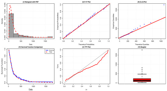
Figure 4. Comparative plots evaluating the adequacy of the AAPEx model on survival times for the data of 45 head and neck cancer patients.

The maximum likelihood estimates (MLEs) and the GoF statistics, along with the corresponding p-values of the application described in Section 7.1 for the fitted models, including the AAPEx distribution and other competing distributions, are presented in Table 6. The negative logarithm and the information criteria are reported in Table 7. The results show that the AAPEx distribution has the smallest values of A*, W* and K-S, along with the largest p-value. This confirms that it provides a superior fit to the survival data compared to other models evaluated in the study.

Table 6. MLEs With GoF statistics for 45 patients with head and neck cancer disease.

Model	$\widehat{\mathit{\alpha }}$	$\widehat{\mathit{\gamma }}$	$\widehat{\mathit{\eta }}$	${\mathit{A}}^{*}$	${\mathit{W}}^{*}$	KS	p-Value
AAPEx	22.64502	1.74971	0.01477	0.11854	0.01329	0.04823	0.99978
Ex	–	–	0.04557	1.02506	0.18737	0.14458	0.27615
EEx	0.04740	–	1.06055	1.08472	0.20649	0.14831	0.24971
W	0.93485	–	21.13857	0.90881	0.14610	0.12894	0.40838
SEx	–	–	0.02536	1.29298	0.25148	0.15813	0.18911
G	1.01382	–	0.04620	1.04062	0.19250	0.14580	0.26730
APEx	0.00985	–	0.01289	0.69647	0.09408	0.10812	0.62967
KwEx	1.35157	0.34143	0.14464	1.30992	0.26539	0.15490	0.20763
MoEx	0.47828	–	0.03000	0.87013	0.12745	0.11055	0.60213

Table 7. The negative logarithm and the information criteria results for 45 patients with head and neck cancer disease.

Model	$-\mathit{\ell }$	AIC	SIC	AICC	HQIC
AAPEx	179.2323	364.4645	369.8845	373.2450	366.4850
Ex	183.9857	369.9714	371.7780	374.1574	370.6449
EEx	183.9450	371.8899	375.5032	378.3185	373.2369
W	183.7745	371.5489	375.1623	377.9775	372.8960
SEx	184.7475	371.4951	373.3017	375.6811	372.1686
G	183.9830	371.9659	375.5793	378.3945	373.3129
APEx	182.1599	368.3198	371.9332	374.7484	369.6668
KwEx	183.5517	373.1034	378.5234	381.8839	375.1239
MoEx	182.9520	369.9040	373.5173	376.3325	371.2510

7.2. Application 2: Remission Times of 36 Bladder Cancer Patients

The second application represents the remission times (in months) for 36 patients diagnosed with bladder cancer, as already analyzed by Reference [19]. The dataset is fully observed, meaning that all remission times are complete, with no censored or truncated observations. No pre-processing was required beyond basic sorting and validation to ensure consistency with the original source. The observations of the dataset are reported in Appendix A.

The summary statistics of the remission times of 36 bladder cancer patients are provided in Table 8. The dataset is negatively skewed, as the skewness value is less than 0. The kurtosis value is less than 3, indicating that the dataset is platykurtic.

Table 8. Summary statistics of 36 patients diagnosed with bladder cancer disease.

N	Min	Max	Mean	Median	SD	CV	Skewness	Kurtosis
36	0.08	3.36	1.94	2.08	0.99	0.51	−0.30	1.86

The maximum likelihood estimates (MLEs) and the GoF statistics, along with the corresponding p-values of the application described in Section 7.2 for the fitted models, including the AAPEx distribution and other competing distributions, are presented in Table 9. The negative logarithm and the information criteria are reported in Table 10. The results show that the AAPEx distribution has the smallest values of A*, W* and K-S, along with the largest p-value. This confirms that it provides a superior fit to the bladder cancer data compared to other models evaluated in this study.

Table 9. MLEs With GoF statistics for 36 patients with bladder cancer disease.

Model	$\widehat{\mathit{\alpha }}$	$\widehat{\mathit{\gamma }}$	$\widehat{\mathit{\eta }}$	${\mathit{A}}^{*}$	${\mathit{W}}^{*}$	KS	p-Value
AAPEx	0.03581	0.65653	1.51556	0.71798	0.10516	0.11153	0.76174
Ex	–	–	0.51546	3.40831	0.65556	0.23032	0.04388
EEx	0.81237	–	2.27235	1.48294	0.25693	0.19628	0.12482
W	1.95698	–	2.16448	1.10604	0.17472	0.16587	0.27522
SEx	–	–	0.29213	3.07562	0.58929	0.22767	0.04789
G	2.30964	–	1.19053	1.40628	0.24106	0.19445	0.13137
APEx	57.9466	–	1.01115	1.03185	0.16795	0.16679	0.26915
KwEx	1.95798	100.005	0.01379	1.11289	0.17745	0.16812	0.26076
MoEx	17.1667	–	1.49380	0.76685	0.10965	0.11438	0.73394

Table 10. The negative logarithm and the information criteria results for 36 patients with bladder cancer.

Model	$-\mathit{\ell }$	AIC	SIC	AICC	HQIC
AAPEx	50.16594	106.3319	111.0824	115.3319	107.9901
Ex	59.85677	121.7135	123.2971	125.9488	122.2662
EEx	54.82474	113.6495	116.8165	120.1949	114.7549
W	51.38705	106.7741	109.9411	113.3195	107.8795
SEx	58.48822	118.9764	120.5599	123.2117	119.5291
G	54.09240	112.1848	115.3518	118.7303	113.2903
APEx	52.58815	109.1763	112.3433	115.7217	110.2817
KwEx	51.51497	109.0299	113.7805	118.0299	110.6880
MoEx	54.24223	108.4845	112.6515	116.0299	109.5898

The TTT-transform plot of the data shows a concave pattern above the 45° line, providing insight into the shape of the hazard function, as shown in Figure 3, and no outlier is revealed in the boxplot illustrated in Figure 5.

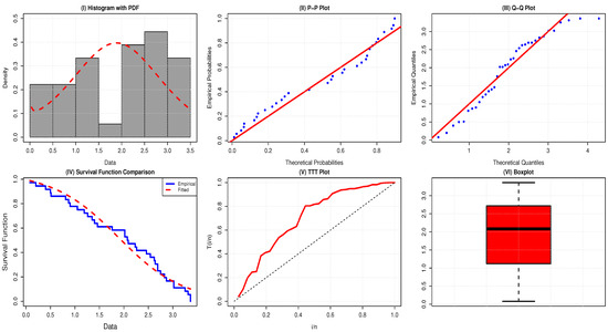
Figure 5. Comparative plots for evaluation of the adequacy of the AAPEx model on remission times for the data of 36 bladder cancer patients.

7.3. Application 3: Remission Times of 128 Bladder Cancer Patients

The third application, comprising uncensored remission times (in months) for 128 patients diagnosed with bladder cancer, exhibits a pronounced right-skewed distribution, as discussed by Reference [20]. The remission times are presented in Appendix A.

The summary statistics of the remission times of 128 bladder cancer patients are provided in Table 11. The dataset is positively skewed and leptokurtic (skewness = 3.32 and kurtosis = 16.15).

Table 11. Summary statistics of 128 patients diagnosed with bladder cancer.

N	Min	Max	Mean	Median	SD	CV	Skewness	Kurtosis
128	0.08	79.05	9.37	6.40	10.51	1.12	3.32	16.15

The maximum likelihood estimates (MLEs) and the GoF statistics with respective p-values of the application described Section 7.3 are exhibited in Table 12. The information criteria and negative logarithm are provided in Table 13. All results indicate that the proposed model possesses the smallest A*, W* and K-S values, in addition to having the largest p-value. This attests to the fact that it offers the best fit of the bladder cancer data among models assessed in this study.

Table 12. MLEs With GoF statistics for 128 patients with bladder cancer.

Model	$\widehat{\mathit{\alpha }}$	$\widehat{\mathit{\gamma }}$	$\widehat{\mathit{\eta }}$	${\mathit{A}}^{*}$	${\mathit{W}}^{*}$	KS	p-Value
AAPEx	4.53731	1.65111	0.07081	95.5586	16.45183	0.03508	0.99749
Ex	–	–	0.10677	98.08299	17.20577	0.08463	0.31835
EEx	0.12117	–	1.21795	108.7662	18.26517	0.07251	0.51132
W	1.04784	–	9.56069	102.4439	17.60350	0.07002	0.55696
SEx	–	–	0.05974	103.4375	17.67466	0.07130	0.53327
G	1.17251	–	0.12519	107.2713	18.10190	0.07329	0.49738
APEx	1.17389	–	0.11132	99.81774	17.35312	0.07934	0.39612
KwEx	1.39231	0.36887	0.31797	109.6697	18.41134	0.07131	0.53309
MoEx	1.05580	–	0.10986	99.23212	17.30257	0.08113	0.36848

Table 13. The negative logarithm and the information criteria results for 128 patients with bladder cancer.

Model	$-\mathit{\ell }$	AIC	SIC	AICC	HQIC
AAPEx	409.3431	824.6862	832.2422	832.9442	828.1625
Ex	414.3419	830.6838	833.5358	834.7473	831.8426
EEx	413.0776	830.1552	835.8592	836.2992	832.4728
W	414.0869	832.1738	837.8778	838.3178	834.4913
SEx	414.3326	830.6652	833.5172	834.7287	831.8240
G	413.3678	830.7356	836.4396	836.8796	833.0531
APEx	414.3182	832.6364	838.3404	838.7804	834.9540
KwEx	412.5467	831.0934	839.6495	839.3515	834.5698
MoEx	414.3262	832.6523	838.3564	838.7963	834.9699

The TTT plot of Dataset 3 is S-shaped—first convex below the ${45}^{\circ }$ line, then concave above it. This suggests a bathtub-shaped hazard rate, with decreasing, constant, then increasing failure rates over time, as shown in Figure 6.

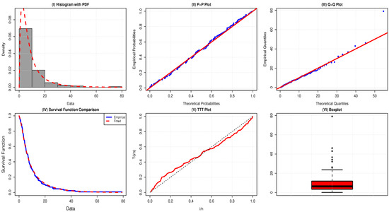
Figure 6. Comparative plots for evaluation of the adequacy of the AAPEx model on remission times for the data of 128 bladder cancer patients.

7.4. Application 4: United Kingdom COVID-19 Mortality Rate Data

The fourth real-life application involves a dataset comprising COVID-19 mortality rates in the United Kingdom. This dataset was previously utilized by References [21,22]. The data were originally retrieved from the World Health Organization (WHO) COVID-19 [https://covid19.who.int/], which provides official global statistics on COVID-19 cases and deaths. The dataset is fully observed, with no censored or truncated values, and each observation represents a recorded mortality rate at a specific time point. Prior to analysis, basic preprocessing steps such as sorting and validation against the WHO database were performed to ensure consistency and accuracy.

Table 14 reports the summary statistics of the UK COVID-19 death rate data. The positive skewness means that the dataset is skewed to the right, and the kurtosis of less than 3 implies that it is platykurtic. The failure rate is of a bathtub shape, since the TTT-transform plot is first convex (below the 45° line), then concave (above the 45° line). Moreover, the boxplot indicates the existence of a few outliers, as shown in Figure 7.

Table 14. Summary statistics of United Kingdom COVID-19 mortality rate data.

N	Min	Max	Mean	Median	SD	CV	Skewness	Kurtosis
76	0.0587	11.4584	2.44	1.25	2.94	1.20	1.73	2.32

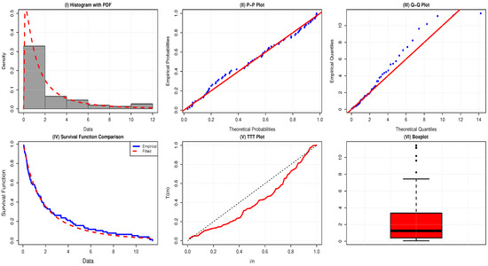
Figure 7. Visual evaluation of the AAPEx model fitted to mortality rates of 76 UK COVID-19 patients.

The MLEs and the GoF statistics, along with corresponding p-values of the application described in Section 7.4, are reported in Table 15. The negative logarithm and information criteria are given in Table 16. The results reveal that the proposed model possesses the minimum values of A*, W* and K-S, along with the maximum p-value. This verifies that it yields a better fit to the COVID-19 mortality data than other models that were tested in this study.

Table 15. MLEs with GoF statistics for United Kingdom COVID-19 mortality rate data.

Model	$\widehat{\mathit{\alpha }}$	$\widehat{\mathit{\gamma }}$	$\widehat{\mathit{\eta }}$	${\mathit{A}}^{*}$	${\mathit{W}}^{*}$	KS	p-Value
AAPEx	4.18814	1.14796	0.21729	11.56824	2.08806	0.06201	0.93198
Ex	–	–	0.41031	15.18011	2.55809	0.14469	0.08295
EEx	0.35303	–	0.80094	12.36936	2.17238	0.09854	0.45159
W	0.84659	–	2.22001	11.68762	2.07868	0.08055	0.70739
SEx	–	–	0.22504	16.91311	2.79431	0.16798	0.02743
G	0.80374	–	0.32978	12.27718	2.15886	0.09615	0.48331
APEx	0.15208	–	0.25403	12.04856	2.13596	0.08109	0.69971
KwEx	0.84519	162.077	0.00108	11.69360	2.07978	0.08094	0.70182
MoEx	0.36165	–	0.24004	11.69679	2.10325	0.07129	0.90182

Table 16. The negative logarithm and the information criteria results for United Kingdom COVID-19 mortality rate data.

Model	$-\mathit{\ell }$	AIC	SIC	AICC	HQIC
AAPEx	139.9784	285.9568	292.9490	294.4013	288.7513
Ex	143.7044	289.4088	291.7395	293.5169	290.3402
EEx	142.5029	289.0059	293.6673	295.2524	290.8688
W	141.7519	287.5037	292.1652	293.7503	289.3667
SEx	145.6999	293.3997	295.7305	297.5079	294.3312
G	142.4105	288.8209	293.4824	295.0675	290.6839
APEx	140.8746	285.7492	290.4107	291.9958	287.6122
KwEx	141.7632	289.5265	296.5187	297.9709	292.3209
MoEx	141.3077	286.6154	293.5187	295.9709	289.3209

7.5. Application 5: Failure Time of Censored Lifetime Data

The fifth application, presented in the Appendix A, involves a dataset of 30 items tested under a Type-II censoring scheme, where the test is terminated after the $20\mathrm{th}$ failure. This dataset was previously utilized by [21,22].

Table 17 reports the summary statistics of the failure time of censored lifetime data. The dataset is almost symmetric, with skewness = 0.0025 and a kurtosis value of less than 3, which implies that it is platykurtic. The failure rate is of a bathtub shape, since the TTT-transform plot is first convex (below the 45° line), then concave (above the 45° line). Moreover, the boxplot indicates the existence of a few outliers, as shown in Figure 8.

Table 17. Summary statistics of failure time of censored lifetime data.

N	Min	Max	Mean	Median	SD	CV	Skewness	Kurtosis
20	0.0014	10.7582	5.42	5.36	3.44	0.63	0.0025	1.87

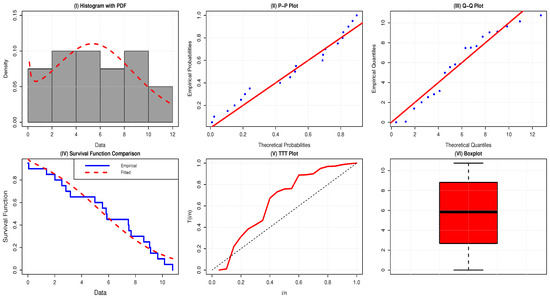
Figure 8. Visual evaluation of the AAPEx model fitted to mortality rates of 76 UK COVID-19 patients.

The maximum likelihood estimates (MLEs) and goodness-of-fit (GoF) statistics, along with their corresponding p-values for the application described in Section 7.5, are presented in Table 18. The negative log-likelihood and associated information criteria are summarized in Table 19. The results demonstrate that the proposed model achieves the lowest values for the A*, W* and K–S test statistics, accompanied by the highest p-value among all the competing models. These findings confirm that the proposed model provides a superior fit to the failure time of censored lifetime data compared to the alternative models considered in this study.

Table 18. MLEs with GoF statistics for failure time of censored lifetime data.

Model	$\widehat{\mathit{\alpha }}$	$\widehat{\mathit{\gamma }}$	$\widehat{\mathit{\eta }}$	${\mathit{A}}^{*}$	${\mathit{W}}^{*}$	KS	p-Value
AAPEx	0.00843	0.08342	0.41587	0.48125	0.06164	0.13795	0.79243
Ex	–	–	0.17519	1.70189	0.26703	0.23231	0.19687
EEx	0.15701	–	0.83773	1.88151	0.33551	0.24932	0.13961
W	1.08926	–	5.81639	1.59742	0.22706	0.22047	0.24651
SEx	–	–	0.09836	1.56546	0.23413	0.22178	0.24059
G	0.86369	–	0.15130	1.84426	0.32241	0.24603	0.14952
APEx	12.40703	–	0.28199	1.13144	0.10865	0.16304	0.60540
KwEx	0.30718	0.05988	2.74289	1.59080	0.30764	0.23903	0.17242
MoEx	8.08609	–	0.39842	1.05247	0.07825	0.14723	0.72520

Table 19. The negative logarithm and the information criteria results for failure time of censored lifetime data.

Model	$-\mathit{\ell }$	AIC	SIC	AICC	HQIC
AAPEx	48.1684	102.3368	105.3239	112.3368	102.9199
Ex	54.8377	111.6754	112.6711	116.1199	111.8698
EEx	54.6205	113.2411	115.2325	120.2999	113.6298
W	54.7518	113.5036	115.4950	120.5624	113.8923
SEx	54.2871	110.5741	111.5699	115.0186	110.7685
W	54.6896	113.3792	115.3707	120.4380	113.7679
APEx	52.9431	109.8862	111.8777	116.9450	110.2750
KwEx	52.5538	111.1076	114.0948	121.1076	111.6907
MoEx	51.8900	107.7801	109.7715	114.8389	108.1688

8. Concluding Remarks

This work advances statistical modeling through the development of the AAP-X family, a novel class of continuous distributions designed to address the inflexibility of classical models. Focusing on its exponential subclass, termed the AAPEx model, we resolve critical limitations of the traditional exponential distribution—most notably, its constant hazard rate—by introducing a shape parameter that enables more flexible hazard function modeling. The AAPEx framework supports increasing, decreasing and bathtub-shaped hazard rates, making it well-suited for complex real-world phenomena.

To lay the theoretical groundwork for the AAPEx model, we derived its structural properties, including moments, quantile functions and hazard-rate behavior. Through extensive Monte Carlo simulations, six frequentist estimation approaches (MLE, CVME, MPSE, OLSE, WLSE and ADE) were systematically implemented and compared. Practical applicability was demonstrated through four real-world datasets, including survival times of cancer patients and COVID-19 mortality rates. In all cases, the AAPEx model provided a superior fit compared to several established competing distributions, as measured by standard goodness-of-fit metrics.

This study is based on the following key assumptions: (i) the data are assumed to be independent and identically distributed (i.i.d.); (ii) the model employs a parametric form for the baseline distribution, such as the exponential; and (iii) the shape parameter ($\gamma$) is well-defined and governs the distribution’s flexibility. Despite its strengths, the model may face convergence issues with small samples and computational challenges with large datasets, particularly in parameter estimation.

Future research can focus on several promising directions. These include extending the AAP-X model to incorporate survival regression structures for enhanced time-to-event analysis, developing multivariate and time-dependent versions and exploring Bayesian estimation methods to improve flexibility and quantify uncertainty. Furthermore, integrating machine learning techniques could significantly enhance the efficiency and scalability of the model, especially in high-dimensional data settings.

References

- Mudholkar, G.S.; Srivastava, D.K. Exponentiated Weibull family for analyzing bathtub failure-rate data. IEEE Trans. Reliab. 1993, 42, 299–302. [Google Scholar] [CrossRef]
- Marshall, A.W.; Olkin, I. A new method for adding a parameter to a family of distributions with application to the exponential and Weibull families. Biometrika 1997, 84, 641–652. [Google Scholar] [CrossRef]
- Mahdavi, A.; Kundu, D. A new method for generating distributions with an application to exponential distribution. Commun. Stat.-Theory Methods 2017, 46, 6543–6557. [Google Scholar] [CrossRef]
- Lone, M.A.; Dar, I.H.; Jan, T. A new family of generalized distributions with an application to weibull distribution. Thail. Stat. 2024, 22, 1–16. [Google Scholar]
- Shah, Z.; Khan, D.M.; Khan, I.; Ahmad, B.; Jeridi, M.; Al-Marzouki, S. A novel flexible exponent power-X family of distributions with applications to COVID-19 mortality rate in Mexico and Canada. Sci. Rep. 2024, 14, 8992. [Google Scholar] [CrossRef] [PubMed]
- Alzaatreh, A.; Lee, C.; Famoye, F. A new method for generating families of continuous distributions. Metron 2013, 71, 63–79. [Google Scholar] [CrossRef]
- Musekwa, R.R.; Gabaitiri, L.; Makubate, B. A New Technique to Generate Families of Continuous Distributions. Colomb. J. Stat. Colomb. Estad. 2024, 47, 329–354. [Google Scholar] [CrossRef]
- Alsolmi, M.M. A New Logarithmic Tangent-U Family of Distributions with Reliability Analysis in Engineering Data. Comput. J. Math. Stat. Sci. 2025, 4, 258–282. [Google Scholar] [CrossRef]
- Odhah, O.H.; Alshanbari, H.M.; Ahmad, Z.; Khan, F.; El-Bagoury, A.a.A.H. A New Family of Distributions Using a Trigonometric Function: Properties and Applications in the Healthcare Sector. Heliyon 2024, 10, e29861. [Google Scholar] [CrossRef] [PubMed]
- Mir, A.A.; Rasool, S.U.; Ahmad, S.; Bhat, A.; Jawa, T.M.; Sayed-Ahmed, N.; Tolba, A.H. A Robust Framework for Probability Distribution Generation: Analyzing Structural Properties and Applications in Engineering and Medicine. Axioms 2025, 14, 281. [Google Scholar] [CrossRef]
- Semary, H.; Hussain, Z.; Hamdi, W.A.; Aldahlan, M.A.; Elbatal, I.; Nagarjuna, V.B. Alpha–beta-power family of distributions with applications to exponential distribution. Alex. Eng. J. 2024, 100, 15–31. [Google Scholar] [CrossRef]
- Balakrishnan, K. Exponential Distribution: Theory, Methods and Applications; CRC Press: Boca Raton, FL, USA, 1996. [Google Scholar]
- Gupta, R.D.; Kundu, D. Exponentiated exponential family: An alternative to gamma and Weibull distributions. Biom. J. J. Math. Methods Biosci. 2001, 43, 117–130. [Google Scholar] [CrossRef]
- Isa, A.M.; Bashiru, S.O.; Ali, B.A.; Adepoju, A.A.; Itopa, I.I. Sine-exponential distribution: Its mathematical properties and application to real dataset. UMYU Sci. 2022, 1, 127–131. [Google Scholar]
- Nassar, M.; Afify, A.Z.; Shakhatreh, M. Estimation methods of alpha power exponential distribution with applications to engineering and medical data. Pak. J. Stat. Oper. Res. 2020, 16, 149–166. [Google Scholar] [CrossRef]
- Adepoju, K.; Chukwu, O. Maximum likelihood estimation of the Kumaraswamy exponential distribution with applications. J. Mod. Appl. Stat. Methods 2015, 14, 18. [Google Scholar] [CrossRef]
- Sule, I.; Doguwa, S.I.; Isah, A.; Jibril, H.M. The topp leone kumaraswamy-g family of distributions with applications to cancer disease data. J. Biostat. Epidemiol. 2020, 6, 40–51. [Google Scholar] [CrossRef]
- Abo-Kasem, O.; Ibrahim, O.; Aljohani, H.M.; Hussam, E.; Kilai, M.; Aldallal, R. Statistical Analysis Based on Progressive Type-I Censored Scheme From Alpha Power Exponential Distribution With Engineering and Medical Applications. J. Math. 2022, 2022, 3175820. [Google Scholar] [CrossRef]
- Hibatullah, R.; Widyaningsih, Y.; Abdullah, S. Marshall-Olkin extended power Lindley distribution with application. J. Ris. Apl. Mat. 2018, 2, 84–92. [Google Scholar] [CrossRef]
- Lee, E.T.; Wang, J. Statistical Methods for Survival Data Analysis; John Wiley & Sons: Hoboken, NJ, USA, 2003; Volume 476. [Google Scholar]
- Kilai, M.; Waititu, G.A.; Kibira, W.A.; Alshanbari, H.M.; El-Morshedy, M. A new generalization of Gull Alpha Power Family of distributions with application to modeling COVID-19 mortality rates. Results Phys. 2022, 36, 105339. [Google Scholar] [CrossRef] [PubMed]
- Kargbo, M.; Gichuhi, A.W.; Wanjoya, A.K. A novel extended inverse-exponential distribution and its application to COVID-19 data. Eng. Rep. 2024, 6, e12828. [Google Scholar] [CrossRef]
Disclaimer/Publisher’s Note: The statements, opinions and data contained in all publications are solely those of the individual author(s) and contributor(s) and not of MDPI and/or the editor(s). MDPI and/or the editor(s) disclaim responsibility for any injury to people or property resulting from any ideas, methods, instructions or products referred to in the content. |
© 2025 by the authors. Licensee MDPI, Basel, Switzerland. This article is an open access article distributed under the terms and conditions of the Creative Commons Attribution (CC BY) license (https://creativecommons.org/licenses/by/4.0/).