On the Evaluation of Rectangular Matrix Permanents: A Symmetric and Combinatorial Analysis

Abstract

This paper presents a combinatorial perspective on evaluating the permanent for a rectangular matrix. It proves that the permanent can be computed using the permanents of its largest square submatrices. The proof employs a structured combinatorial method and reveals a connection to the subset-sum problem, known as the grid shading problem. Furthermore, this study uncovers an inherent symmetry in the distribution of terms, highlighting structured patterns within permanent computation. This perspective bridges combinatorial principles with matrix theory, offering new insights into their interplay.

1. Introduction

In matrix theory, the permanent is a function of matrices that differs from the determinant primarily in its omission of permutation signs. While the determinant has a well-established strong geometric interpretation, the permanent has no such perspective. This distinction extends to their computational complexity; computing the determinant is polynomial time, while computing the permanent is computationally challenging, classified as a #P-complete problem. Despite their differences, both functions share a common combinatorial structure, being defined through summations over permutations. Let $A=\left[a_{ij}\right]$ be a matrix of size m by n with elements in a field F and suppose that $m\le n$. Then, the permanent and determinant of A are defined as follows [1]:

$$\mathrm{per}\left(A\right)=\sum _{\sigma }{a}_{1{\sigma }_1}{a}_{2{\sigma }_2}\dots a_{m{\sigma }_m}$$

(1)

and

$$\det \left(A\right)=\sum _{\sigma }sgn\left(\sigma \right)a_{1{\sigma }_1}{a}_{2{\sigma }_2}\dots a_{m{\sigma }_m}$$

(2)

where the summations runs over on the set $\sigma$, which includes all one-to-one functions defined from $\{1,2,\dots ,m\}$ to $\{1,2,\dots ,n\}$. The only difference between these definitions is the inclusion of the permutation sign, $\mathrm{sgn}\left(\sigma \right)$, in the determinant. However, this seemingly small distinction has major implications for their properties and computational feasibility. While significant progress has been made in the efficient computation of the determinants using various algebraic methods, the inherent complexity of the permanent has motivated researchers to explore alternative approaches. This has led to extensive research into new approaches for evaluating the permanent. A review of recent theoretical developments follows.

Björklund et al. [2] approached the permanent evaluation problem using combinatorial and algebraic techniques. Their work emphasizes dynamic programming methods that compute intermediate results by constructing tables over subsets of column indices. Additionally, they extend Ryser’s permanent formula by presenting an optimized version for rectangular matrices, significantly improving its computational performance. These contributions provide theoretical insights that align with the subset-based combinatorial framework developed in this study.

Recent studies have also explored quantum-inspired approaches to permanent computation. For instance, Troyansky and Tishby [3] constructed a quantum observable whose expectation value yields the permanent (for bosons) or determinant (for fermions) of a matrix, emphasizing the intrinsic variance in quantum measurements, which corresponds to the computational complexity gap between permanents and determinants. Similarly, Chabaud et al. [4] employed quantum-inspired techniques to provide swift proofs of many important theorems about the permanent, such as the MacMahon Master Theorem.

Masschelein’s work [5] extends Glynn’s algorithm to rectangular matrices and integrates it into a computational framework that dynamically selects the optimal algorithm—Naive, Ryser’s, or Glynn’s—based on the matrix’s properties. Similarly, Niu et al. [6] introduced an algorithm for square matrices that constructs the permanent through submatrices. However, their work is limited to square matrices and emphasizes algorithmic efficiency over theoretical advancements.

In addition to algorithmic approaches, symbolic and algebraic methods have also been instrumental in advancing permanent computation. Chakraborty et al. [7] employed symbolic techniques and dynamic programming to improve permanent computation for dense and structured matrices. Spies [8] provided an algebraic reformulation of Ryser’s formula using polynomial expansions, offering new insights into the combinatorial structure of the permanent. Similarly, Callan [9] explored Möbius inversion and trigonometric properties to derive closed-form solutions for specific matrix classes, contributing to the theoretical understanding of permanent computation.

Baykasoglu [10] provided a graphical interpretation of permanent computation using directed graphs and subgraph enumeration. This alternative representation highlights the structural complexity of permanents and offers new insights into their combinatorial properties. The graphical approach is particularly useful for visualizing how terms in Ryser’s formula correspond to different structural patterns within the matrix.

The computation of determinants for rectangular matrices has been considered through various approaches. Cullis [11] pioneered the study of determinant computation for non-square matrices using the determinants of sub-square matrices, a problem later explored by Radic [12] and Joshi [13]. Joshi’s work, in particular, introduced a combinatorial method for evaluating determinants of rectangular matrices, which serves as a conceptual framework relevant to this study. His determinant algorithm exhibits a combinatorial structure similar to the approach in this study. The method begins with a selection of elements from the matrix and proceeds by arranging columns into a specific order to determine the determinant recursively. This method will be described in detail in the next section.

Our study aims to provide evidence that the evaluation of the permanent of a rectangular matrix can be performed using its square submatrices. While adapting existing determinant methods for non-square matrices may seem natural, such approaches are devoid of a direct theoretical basis. To fill this gap, we introduce a rigorous combinatorial framework specifically designed for the permanence of rectangular matrices. This framework bridges combinatorics and matrix analysis while linking the evaluation of the permanent to a subset-sum problem, providing a novel perspective.

2. Background and Notation

The problem of evaluating the permanent of a rectangular matrix has been addressed using different approaches, ranging from classical algebraic formulations to algorithmic improvements. In this section, we provide an overview of the existing methodologies and introduce the basic notation used in our analysis.

Binet [14], who is credited with introducing the definition of the permanent, initially restricted it to matrices of orders $m\in \{2,3,4\}$, defining it as the sum of all possible products of m elements, with no two elements from the same row or column. Minc [15] later generalized Binet’s definition to matrices of arbitrary finite orders m and n, formalizing it in Equation (1).

The study of permanents for rectangular matrices has gained interest, particularly following Ryser’s work [16], which introduced a formula based on the Inclusion–Exclusion principle. This formula, known as Ryser’s theorem, is as follows:

Let A be a matrix of size $m\times n$ with $m\le n$. Let $A_r$ denote a matrix obtained from A by replacing r columns of A by zeros. Let $S\left(A_r\right)$ denote the product of the row sums of $A_r$, and let $\mathrm{\Sigma }S\left(A_r\right)$ denote the sums of the $S\left(A_r\right)$ over all of the choices for $A_r$. Then,

$$\begin{array}{cc}\hfill \mathrm{per}\left(A\right)& =\mathrm{\Sigma }S\left(A_{n-m}\right)-\left({\displaystyle \begin{array}{c}n-m+1\\ 1\end{array}}\right)\mathrm{\Sigma }S\left(A_{n-m+1}\right)+\left({\displaystyle \begin{array}{c}n-m+2\\ 2\end{array}}\right)\mathrm{\Sigma }S\left(A_{n-m+2}\right)-\dots \hfill \\ & \cdots +{(-1)}^{m-1}\left({\displaystyle \begin{array}{c}n-1\\ m-1\end{array}}\right)\mathrm{\Sigma }S\left(A_{n-1}\right).\hfill \end{array}$$

Minc [15] observed and claimed that, although the Inclusion–Exclusion principle is formally established by Ryser, the foundational structure of permanent evaluation, as initially introduced by Binet, was inherently compatible with this idea. Binet formulated the permanents of $m\times n$ matrices under the restriction $m\le 4$. Building on this, Minc further refined and simplified Ryser’s formula, leading to the following expression in [17]:

$$\mathrm{per}\left(A\right)=\prod _{i=1}^m{r}_i\left(A\right)+\sum _{t=1}^{m-1}{c}_t\sum _{X\in {\Lambda }_{m-t}}\prod _{i=1}^m{r}_i\left(X\right)$$

where $c_1=-1$ and $c_t=-1-{\sum }_{r=1}^{t-1}\left({\displaystyle \begin{array}{c}n-m+t\\ t-r\end{array}}\right)c_r,t=2,\dots ,m-1$.

In [17], Minc presents another formula for computing the permanent of an $m\times n$ matrix, $m\le n$, expressed in terms of the R functions, which is formally stated as the following theorem:

Let A be an $m\times n$ matrix, $2\le m\le n$. Then,

$$\mathrm{per}\left(A\right)=\sum _{\omega \in D\left(m\right)}c\left(\omega \right)R\left(\omega \right)$$

where $\omega =({\omega }_1,\dots ,{\omega }_k)\in D\left(m\right) \mathrm{and} c\left(\omega \right)={(-1)}^{m+k}{\prod }_{i=1}^k({\omega }_i-1)!.$

In this formula, $D\left(m\right)$ denotes the set of increasing sequences of positive integers $(t_1,\dots ,t_k)$ such that $t_1+\cdots +t_k=m$. For $(t_1,\dots ,t_k)\in D\left(m\right)$ the R-function $R(t_1,\dots ,t_k)$ is the symmetrized sum of all distinct products of the $r_{i_1},\dots ,r_{i_j}$ so that in each product the sequences $(i_1,\dots ,i_j)\in Q_{i_j,m},j=1,\dots ,k$, partition the set $\{1,\dots ,m\}$.

In [18], Bebiano noted that the permanent of a rectangular $m\times n$ matrix $A,m\le n$, can be obtained by evaluating the permanent of the $n\times n$ matrix

$$B=\left[\begin{array}{c}A\\ C\end{array}\right],$$

where C is the $(n-m)\times n$ matrix all of whose entries are 1. Then,

$$\mathrm{per}\left(B\right)=(n-m)!\mathrm{per}\left(A\right).$$

As mentioned in the Introduction, we will also consider approaches for rectangular determinants. In this context, we will focus on Joshi’s method for rectangular determinant evaluation. Joshi’s rectangular determinant algorithm exhibits a combinatorial structure, similar to the approach in this study. The method begins with a selection of elements from the matrix and proceeds by arranging columns into a specific order to determine the determinant recursively. Joshi has provided the following formula for evaluating the determinant in [13].

For an $m\times n$ matrix A with real entries, let $A_p^d$ be defined as above; then,

$$\det \left(A\right)=\sum _{d=1}^{n-m+1}\sum _{p=1}^{N_d}\det A_p^d.$$

The sub-square matrices used in Joshi’s algorithm are denoted by $A_p^d$. To form the matrices $A_p^d$, m columns from n columns should be selected $\left(m\le n\right)$. The column with the smallest column number among these m columns is labeled as the dth column, where $1\le d\le n-m+1$. Then, the other columns are determined by choosing $m-1$ columns among the ones right of the dth column regarding their order. Thus, each new column is located to the right of the previous column. According to Joshi’s definition, for example, in computing the determinant of a matrix A of order $3\times n$, the submatrices of order $3\times 3$ used are given by the set $\{A_p^i\mid p\le N_d\}$. Here, the index i ranges from 1 to $n-2$. The set $\left\{A_p^1\right\}$ consists of all 3 by 3 submatrices, the first column of which is the first column of matrix A. Similarly, $\left\{A_p^2\right\}$ includes all 3 by 3 submatrices, the first column of which is the second column of matrix A. Following this pattern, $\left\{A_p^{n-2}\right\}$ represents the submatrices, the first column of which is the $(n-2)$th column of matrix A. Therefore, the set $\left\{A_p^{n-2}\right\}$ represents the submatrix formed by the last three columns of matrix A. On the other hand, the columns used to construct the matrices $A_p^d$ are determined by the sets $S_d$. Note that $N_d$ is the maximum value of p, indicating the number of elements in $S_d$. m-tuples which are the elements of $S_d$ sets are denoted as $e_p^d$ which is constructed as $\left(d,k_{p2},k_{p3},\dots ,k_{pm}\right)$ where $1⩽d<k_{p2}<k_{p3}<\dots <k_{pm}⩽n.$ The components other than the first component of these m-tuples are determined from the set $\{d+1,d+2,\dots ,n\}$. Therefore, $S_d$ sets are formed by $e_p^d$’s. There emerge $\left({\displaystyle \begin{array}{c}n-1\\ m-1\end{array}}\right)$ different $e_p^1$’s for $S_1$ set, $\left({\displaystyle \begin{array}{c}n-2\\ m-1\end{array}}\right)$ different $e_p^2$’s for $S_2$ set, and finally $\left({\displaystyle \begin{array}{c}n-d\\ m-1\end{array}}\right)$ different $e_p^d$’s for $S_d$ set. Therefore, $N_1=\left({\displaystyle \begin{array}{c}n-1\\ m-1\end{array}}\right)$, $N_2=\left({\displaystyle \begin{array}{c}n-2\\ m-1\end{array}}\right)$, …, $N_d=\left({\displaystyle \begin{array}{c}n-d\\ m-1\end{array}}\right)$, …, $N_{n-m+1}=1$.

The approach presented in this study differs significantly from those in previous studies, particularly related to the evaluation of permanents and determinants. Unlike prior work, which often relies on algorithmic or recursive formulations, our work introduces an entirely different framework. This framework provides a combinatorial interpretation of the rectangular permanent problem, linking its evaluation to the solution of a structured combinatorial problem. Furthermore, our perspective is designed as a proof-driven approach, aiming to establish a theoretical foundation rather than optimize the permanent computation. The following sections will develop this theoretical basis and demonstrate its consistency through numerical examples.

3. Evaluation of Permanent for Rectangular Matrices

In this section, we provide two proofs demonstrating that the permanent of a rectangular matrix can be computed using the permanents of its largest square submatrices. Our goal is to develop a theoretical analysis of this problem. To illustrate the problem more concretely, we introduce the statement given in the following theorem. Although this statement is not a complete and explicit direct computation formula, it contributes to a better understanding and analysis of the problem under consideration.

Theorem 1.

Let $A=\left[a_{kj}\right]$ be a rectangular matrix of order $m\times n$ with $m\le n$. The permanent of A is given by

$$\mathrm{per}\left(A\right)=\sum _{r=0}^{m(n-m)}\sum _i\mathrm{per}\left(A_{\varphi (r,m),i}\right),$$

(3)

where $A_{\varphi (r,m),i}$ denotes the matrix whose columns are those indexed by the entries of the tuples ${\overrightarrow{j}}_{(r,m)}^i=\left(j_1^i,j_2^i,\dots ,j_m^i\right)$ satisfying

$$j_1^i+j_2^i+\cdots +j_m^i=\varphi (r,m)$$

(4)

where

$$\varphi (r,m)={\displaystyle \frac{m(m+1)}{2}}+r$$

(5)

and the index i ranges over as many numbers as needed to account for all possible m-tuples satisfying the condition (4).

Proof. 

To compute $\mathrm{per}\left(A\right)$, we expand it using the permanent definition given by Equation (1). The resulting expansion consists of $m!\left({\displaystyle \begin{array}{c}n\\ m\end{array}}\right)$ terms. The structure of each term is of the form $a_{1j_1}{a}_{2j_2}\dots a_{m{j}_m}$. These terms are grouped according to the column indices of their constituent factors (i.e., elements of the matrix). Specifically, within each group, the sum of the column indices of the matrix elements forming the terms is identical and satisfies the condition

$$j_1+j_2+\dots +j_m=\varphi (r,m)$$

(6)

where $r=0,1,2,\dots ,m(n-m)$. Using this grouping process, let us express

$$\mathrm{per}\left(A\right)=\sum _{p=1}^{\left({\displaystyle \begin{array}{c}n\\ m\end{array}}\right)}{\mathcal{K}}_p$$

(7)

where each ${\mathcal{K}}_p$ represents a sum of $m!$ terms of the form $a_{1j_1}{a}_{2j_2}\dots a_{m{j}_m}$. For the ${\mathcal{K}}_p$ sums, we provide the following explanations.

${\mathcal{K}}_1$ is associated with $\varphi (0,m)={\displaystyle \frac{m(m+1)}{2}}$. Consequently, it consists of terms indexed by the tuple ${\overrightarrow{j}}_{(0,m)}^1=(1,2,\dots ,m)$, i.e.,

$${\mathcal{K}}_1=\sum _{{\overrightarrow{j}}_{(0,m)}^1\times {\overrightarrow{j}}_{(0,m)}^1}{a}_{1j_1^1}{a}_{2j_2^1}\dots a_{m{j}_m^1}.$$

(8)

Here, the set denoted as ${\overrightarrow{j}}_{(0,m)}^1\times {\overrightarrow{j}}_{(0,m)}^1$ represents the set of all one-to-one functions defined from ${\overrightarrow{j}}_{(0,m)}^1$ to ${\overrightarrow{j}}_{(0,m)}^1$. Accordingly, ${\mathcal{K}}_1$ corresponds to the permanent of the m by m submatrix consisting of the first m columns of matrix A.

${\mathcal{K}}_2$ is associated with $\varphi (1,m)={\displaystyle \frac{m(m+1)}{2}}+1$. It consists of terms indexed by the tuple ${\overrightarrow{j}}_{(1,m)}^1=(1,2,\dots ,m-1,m+1)$, i.e.,

$${\mathcal{K}}_2=\sum _{{\overrightarrow{j}}_{(1,m)}^1\times {\overrightarrow{j}}_{(1,m)}^1}{a}_{1j_1^1}{a}_{2j_2^1}\dots a_{m{j}_m^1}.$$

(9)

This indicates that ${\mathcal{K}}_2$ corresponds to the permanent of the m by m submatrix consisting of the first $m-1$ columns and the $(m+1)$th column of A.

We note that some $\varphi (r,m)$ values can yield multiple ${\overrightarrow{j}}_{(r,m)}^i$ tuples when $n-m>1$. In such cases, multiple ${\mathcal{K}}_p$ summations arise. For instance, the equation $\varphi (2,m)={\displaystyle \frac{m(m+1)}{2}}+2$ gives two distinct m-tuples, under this condition:

$${\overrightarrow{j}}_{(2,m)}^1=(1,2,\dots ,m-1,m+2),$$

(10)

$${\overrightarrow{j}}_{(2,m)}^2=(1,2,\dots ,m-2,m,m+1).$$

(11)

As a result, two different summations,

$${\mathcal{K}}_3=\sum _{{\overrightarrow{j}}_{(2,m)}^1\times {\overrightarrow{j}}_{(2,m)}^1}{a}_{1j_1^1}{a}_{2j_2^1}\dots a_{m{j}_m^1}$$

(12)

and

$${\mathcal{K}}_4=\sum _{{\overrightarrow{j}}_{(2,m)}^2\times {\overrightarrow{j}}_{(2,m)}^2}{a}_{1j_1^2}{a}_{2j_2^2}\dots a_{m{j}_m^2}$$

(13)

are presented. So, ${\mathcal{K}}_3$ corresponds to the permanent of the m by m submatrix consisting of the first $m-1$ columns and the $(m+2)$th column of matrix A. Similarly, ${\mathcal{K}}_4$ corresponds to the permanent of the m by m submatrix formed by the first $m-2$ columns, along with the mth and $(m+1)$th columns of matrix A.

As exemplified for some values of p above, each $K_p$ corresponds to the permanent of a distinct m by m submatrix. The selection of column indices via the grouping procedure determines a unique submatrix $A_{\varphi (r,m),i}$, whose permanent contributes to the summation in Equation (7). This approach ensures that all possible submatrices of order $m\times m$ within A are systematically considered, confirming the completeness of the expansion given by Equation (3).

Note that the summation symbol iterating over the index i arises from the fact that multiple m-tuples are obtained from certain $\varphi (r,m)$. The index i is not explicitly defined in Equation (3), though its iteration count can be easily calculated. The index i serves to illustrate the possible multiple m-tuples formed by ${\overrightarrow{j}}_{(r,m)}^i$ and to make them more noticeable. For a clearer understanding of the i-loop, see Section 4 and Section 5. □

The proof given above utilizes a special grouping process to evaluate the permanent of m by n matrix A, thereby forming the permanents of m by m submatrices. On the other hand, an alternative proof will be presented, in which we employ a generating function approach to systematically count the ${\overrightarrow{j}}_{(r,m)}^i$ tuples corresponding to the values of $\varphi (r,m)$, generating the sub-square permanents.

An Alternative Proof of Theorem 1

Proof. 

Let $S(m,n,\varphi (r,m\left)\right)$ denote the number of distinct ${\overrightarrow{j}}_{(r,m)}^i$ tuples associated with each $\varphi (r,m)$. Additionally, consider the array $\langle S(m,n,{\varphi }_r)\rangle$, which contains the values $J(m,n,{\varphi }_r)$ and consists of $m(n-m)+1$ elements. This array represents a structured mapping of the submatrix selection process based on column index sums. The main objective of this proof is to demonstrate that the equality

$$\sum _{r=0}^{m(n-m)}S(m,n,\varphi \left(r,m\right))=\left({\displaystyle \begin{array}{c}n\\ m\end{array}}\right)$$

(14)

holds.

A detailed examination of the distribution of $\varphi (r,m)$ values reveals a significant symmetry arising from the grouping process defined in the theorem. This symmetry is confirmed by the equality of the sequence sizes:

$$\left|S\right(m,n,\varphi (r,m)\left)\right|=\left|S\right(m,n,\varphi \left(m\right(n-m)-r,m)\left)\right|$$

For example, the sets corresponding to $\varphi (0,m)$ and $\varphi \left(m\right(n-m),m)$ have the same count, as do those for $\varphi (1,m)$ and $\varphi \left(m\right(n-m)-1,m)$. To analyze this distribution further, we apply the generating function approach to count the sets $\{{\overrightarrow{j}}_{(r,m)}^i\}$.

To achieve this, we make use of the function defined in [19], given by

$$G(x,y)=\prod _{j=1}^n\left(1+x^{j}y\right)$$

(15)

where j represents the columns of matrix A. Expanding Equation (15) with respect to y, we obtain

$$G(x,y)=\sum _{m=0}^n{G}_m\left(x\right)y^m$$

(16)

where $G_m\left(x\right)$ is a generating function of the form

$$G_m\left(x\right)=\sum _{r=0}^{m(n-m)}{x}^{{\varphi }_{\left(r,m\right)}}S(m,n,\varphi \left(r,m\right)).$$

(17)

Then, it follows that the equality

$$\underset{x\to 1}{\lim }{G}_m\left(x\right)=\left({\displaystyle \begin{array}{c}n\\ m\end{array}}\right)$$

(18)

corresponds to (14), and this can be proved by induction on n.

For the base case $n=1$, Equation (15) simplifies to

$$G(x,y)=1+xy$$

(19)

while Equation (16) gives $G(x,y)=G_0\left(x\right)+G_1\left(x\right)y$, thus verifying Equation (18) for $n=1$.

Assuming Equation (18) holds for $n=s$, the function $G(x,y)$ for $n=s+1$ can be written as

$${\displaystyle \begin{array}{l}\prod _{j=1}^{s+1}\left(1+x^{j}y\right)=\left(1+xy\right)\left(1+x^{2}y\right)\dots \left(1+x^{s+1}y\right)\\ =\left(G_0\left(x\right)+G_1\left(x\right)y+G_2\left(x\right)y^2+\dots +G_s\left(x\right)y^s\right)\left(1+x^{s+1}y\right)\hfill \\ =G_0\left(x\right)+\left(G_1\left(x\right)+G_0\left(x\right)x^{s+1}\right)y+\left(G_2\left(x\right)+G_1\left(x\right)x^{s+1}\right)y^2+\dots \hfill \\ \dots +\left(G_s\left(x\right)+G_{s-1}\left(x\right)x^{s+1}\right)y^s+G_s\left(x\right)x^{s+1}{y}^{s+1}\hfill \end{array}}$$

(20)

Thus, the coefficient of the term with $y^m$ in the expansion is

$$G_m\left(x\right)+x^{s+1}{G}_{m-1}\left(x\right).$$

(21)

Given that the equality ${\lim }_{x\to 1}{G}_m\left(x\right)=\left({\displaystyle \begin{array}{c}s\\ m\end{array}}\right)$ holds for $n=s$, the corresponding relation ${\lim }_{x\to 1}{G}_{m-1}\left(x\right)=\left({\displaystyle \begin{array}{c}s\\ m-1\end{array}}\right)$ is therefore satisfied. Substituting these equalities into Equation (21) after taking the limit enables the continuation of the proof.

Applying the limit of Equation (21) and substituting the previously established equalities for $n=s$ and $n=s-1$, we obtain

$$\underset{x\to 1}{\lim }\left(G_m\left(x\right)+x^{s+1}{G}_{m-1}\left(x\right)\right)=\left({\displaystyle \begin{array}{c}s\\ m\end{array}}\right)+\left({\displaystyle \begin{array}{c}s\\ m-1\end{array}}\right).$$

(22)

Utilizing Pascal’s identity, this expression simplifies to $\left({\displaystyle \begin{array}{c}s+1\\ m\end{array}}\right)$, thereby completing the proof. □

4. Combinatorial Symmetries in Grid Shading Problem and Rectangular Matrix Permanents

The problem of identifying subsets within a set of integers whose sum equals a specified value k is a well-known form of the subset-sum problem. A specific case of this problem concerns finding subsets that not only satisfy the sum condition but also contain an equal number of elements. This variant introduces additional combinatorial complexity, as it requires balancing the subset cardinality alongside the sum constraint.

The grid shading problem, as introduced in [20], presents a combinatorial approach to subset selection by determining subsets of grid columns based on specific sum conditions. We can use this approach to interpret the combinatorial structure in our study.

In solving the grid shading problem, the author of [20] considered the number of iso-square blocks in an $m\times n$ rectangular grid, where cells are shaded according to a defined rule. Each distinct shading pattern, referred to as a proper shading, corresponds to a unique configuration derived from these sum-based constraints.

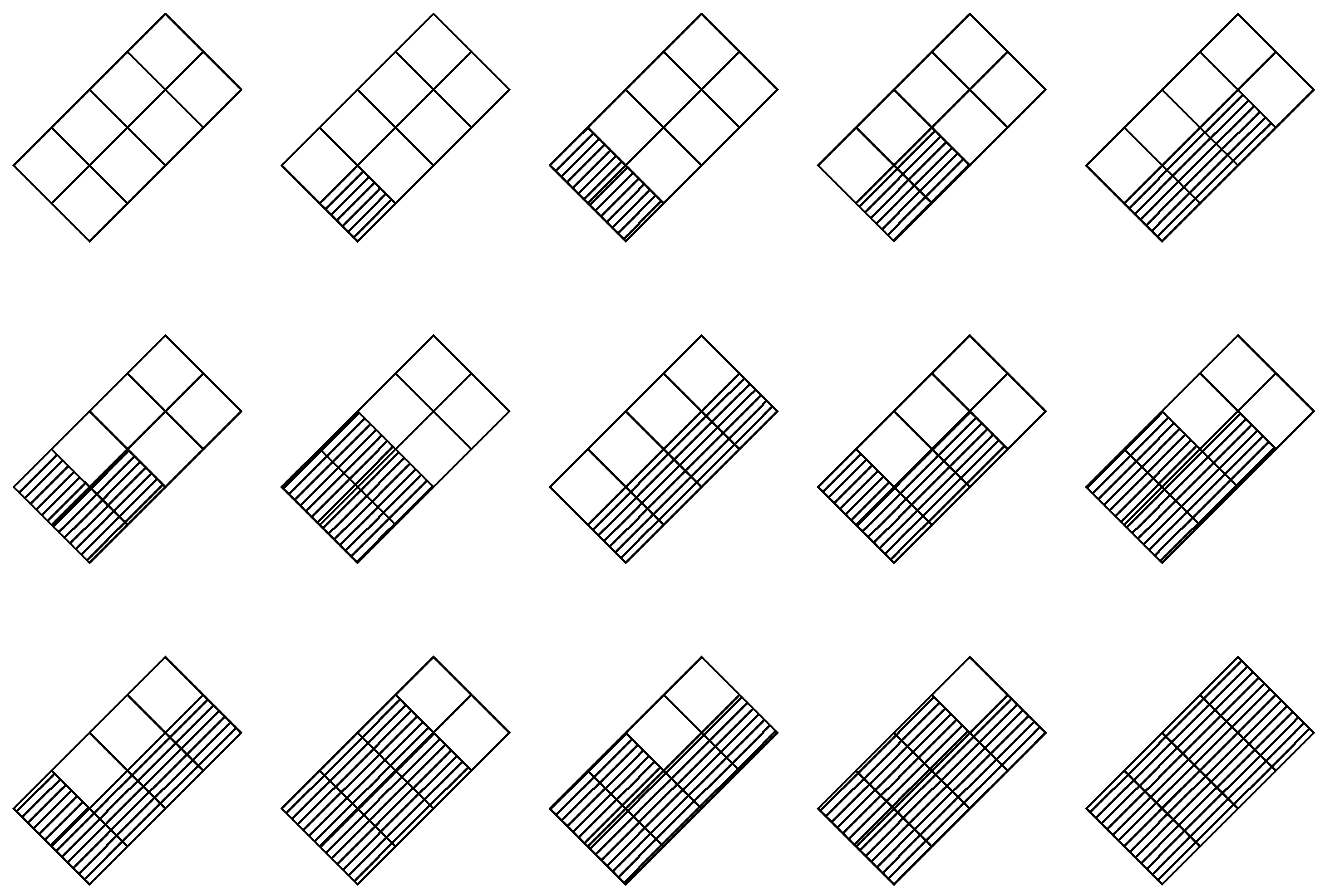
Notably, the number of possible proper shadings exhibits an unimodal sequence, which aligns with the structured sequences that emerge in our method when analyzing submatrices of a given order. For a $2\times 3$ grid, the resulting sequence of proper shadings forms the following unimodal distribution:

$$\left(1,1,2,2,2,1,1\right)$$

(23)

A visualization of this sequence is shown in [20], using a $2\times 3$ grid. Additionally, the following unimodal sequence is formed by the number of proper shadings in the $2\times 4$ grid:

$$\left(1,1,2,2,3,2,2,1,1\right)$$

(24)

We provide the original visualization of this sequence, corresponding to the $2\times 4$ grid, in Figure 1. Similarly, another unimodal sequence

$$\left(1,1,2,3,4,4,5,4,4,3,2,1,1\right)$$

(25)

is formed by the numbers of the proper shadings that can be obtained by the $3\times 4$ grid.

Our procedure for determining submatrices based on the sum of column indices provides a strong connection with Proctor’s grid shading problem [20]. The sequence $\langle S(m,n,\varphi (r,m\left)\right)\rangle$, where $r=0,1,\dots ,m(n-m)$, corresponds precisely to the sequence obtained through proper shadings in an $(n-m)\times m$ grid. This direct correspondence establishes a meaningful combinatorial link between the two problems, reinforcing the foundation of our approach.

For instance, for a $4\times 6$ matrix A, the sequence $\langle S(4,6,\varphi (r,4\left)\right)\rangle$, where $r=0,1,\dots ,8$, corresponds to the sequence obtained by shading a $2\times 4$ grid in Proctor’s problem.

5. Illustrative Example

Consider a matrix A of order $4\times 6$. Based on the condition given by Equation (5), the values of r range among $\{0,1,\dots ,8\}$, leading to the identification of the corresponding submatrices. Then, we obtain the data as in

Table 1. Evaluated values of r, $\varphi (r,4)$, and ${\overrightarrow{j}}_{(r,4)}^i$ for $m=4$, $n=6$.

r	$\mathit{\varphi }(\mathit{r},4)$	${\overrightarrow{\mathit{j}}}_{(\mathit{r},4)}^{\mathit{i}}$	$\mathit{S}(4,6,\mathit{\varphi }(\mathit{r},4\left)\right)$
0	10	$(1,2,3,4)$	1
1	11	$(1,2,3,5)$	1
2	12	$(1,2,4,5)$, $(1,2,3,6)$	2
3	13	$(1,3,4,5)$, $(1,2,4,6)$	2
4	14	$(1,2,5,6)$, $(1,3,4,6)$, $(2,3,4,5)$	3
5	15	$(1,3,5,6)$, $(2,3,4,6)$	2
6	16	$(1,4,5,6)$, $(2,3,5,6)$	2
7	17	$(2,4,5,6)$	1
8	18	$(3,4,5,6)$	1

.

For example, if $r=2$, then ${\varphi }_2=12$. This implies the condition

$$j_1+j_2+j_3+j_4=12,$$

which gives two possible tuples ${\overrightarrow{j}}_{(2,4)}^1=(1,2,4,5)$ and ${\overrightarrow{j}}_{(2,4)}^2=(1,2,3,6)$.

Let us define the following selection principle:

$$j_1\in {\overrightarrow{j}}_{(r,m)}^i, j_2\in {\overrightarrow{j}}_{(r,m)}^i-\left\{j_1\right\}, j_3\in {\overrightarrow{j}}_{(r,m)}^i-\left\{j_1,j_2\right\}, \mathrm{and} j_4\in {\overrightarrow{j}}_{(r,m)}^i-\left\{j_1,j_2,j_3\right\}.$$

The corresponding products of the form $a_{1j_1}{a}_{2j_2}{a}_{3j_3}{a}_{4j_4}$ are then generated according to this principle.

For ${\overrightarrow{j}}_{(2,4)}^1$, all possible quartic products are determined as follows:

• If $j_1=1$, then $j_2\in \{2,4,5\}$. Choosing $j_2=2$ indicates $j_3\in \{4,5\}$, yielding $a_{11}{a}_{22}{a}_{34}{a}_{45}$ and $a_{11}{a}_{22}{a}_{35}{a}_{44}$. For $j_2=4$, $j_3\in \{2,5\}$ yields $a_{11}{a}_{24}{a}_{32}{a}_{45}$ and $a_{11}{a}_{24}{a}_{35}{a}_{42}$. For $j_2=5$, $j_3\in \{2,4\}$ yields $a_{11}{a}_{25}{a}_{32}{a}_{44}$ and $a_{11}{a}_{25}{a}_{34}{a}_{42}$.

• If $j_1=2$, then $j_2\in \{1,4,5\}$. Choosing $j_2=1$ indicates $j_3\in \{4,5\}$, yielding $a_{12}{a}_{21}{a}_{34}{a}_{45}$ and $a_{12}{a}_{21}{a}_{35}{a}_{44}$. For $j_2=4$, $j_3\in \{1,5\}$ yields $a_{12}{a}_{24}{a}_{31}{a}_{45}$ and $a_{12}{a}_{24}{a}_{35}{a}_{41}$. For $j_2=5$, $j_3\in \{1,4\}$ yields $a_{12}{a}_{25}{a}_{31}{a}_{44}$ and $a_{12}{a}_{25}{a}_{34}{a}_{41}$.

• If $j_1=4$, then $j_2\in \{1,2,5\}$. Choosing $j_2=1$ indicates $j_3\in \{2,5\}$, yielding the terms $a_{14}{a}_{21}{a}_{32}{a}_{45}$ and $a_{14}{a}_{21}{a}_{35}{a}_{42}$. For $j_2=2$, $j_3\in \{1,5\}$ yields $a_{14}{a}_{22}{a}_{31}{a}_{45}$ and $a_{14}{a}_{22}{a}_{35}{a}_{41}$. For $j_2=5$, $j_3\in \{1,2\}$ yields $a_{14}{a}_{25}{a}_{31}{a}_{42}$ and $a_{14}{a}_{25}{a}_{32}{a}_{41}$.

• If $j_1=5$, then $j_2\in \{1,2,4\}$. Choosing $j_2=1$ indicates $j_3\in \{2,4\}$, yielding the terms $a_{15}{a}_{21}{a}_{32}{a}_{44}$ and $a_{15}{a}_{21}{a}_{34}{a}_{42}$. For $j_2=2$, $j_3\in \{1,4\}$ yields $a_{15}{a}_{22}{a}_{31}{a}_{44}$ and $a_{15}{a}_{22}{a}_{34}{a}_{41}$. For $j_2=4$, $j_3\in \{1,2\}$ yields $a_{15}{a}_{24}{a}_{31}{a}_{42}$ and $a_{15}{a}_{24}{a}_{32}{a}_{41}$.

The sum of the 24 quartic terms obtained via the set ${\overrightarrow{j}}_{(2,4)}^1$ is denoted by ${\mathcal{K}}_{{\overrightarrow{j}}_{(2,4)}^1}$. According to the permanent definition in Equation (1), the sum ${\mathcal{K}}_{{\overrightarrow{j}}_{(2,4)}^1}$ corresponds to the permanent of the submatrix $A_{\varphi (2,4),1}$ which consists of the first, second, fourth, and fifth columns of matrix A.

From Table 1, we obtain the sequence

$$\langle J\left(4,6,{\varphi }_r\right)\rangle =\left(1,1,2,2,3,2,2,1,1\right)$$

(26)

and so

$$\sum _{r=0,1,\dots ,8}J\left(4,6,{\varphi }_r\right)=15.$$

(27)

Indeed, the number of different submatrices of order $4\times 4$ for a matrix of order $4\times 6$ is $\left({\displaystyle \begin{array}{c}6\\ 4\end{array}}\right)$. Note that the sequence $\langle J\left(4,6,{\varphi }_r\right)\rangle$ overlaps with the sequence obtained by the Proctor’s grid shadings of order $2\times 4$. As a visual representation of these results, Figure 1 showing the $2\times 4$ grid shading patterns is given above.

6. Conclusions

This study establishes a theoretical framework demonstrating that the permanent of a rectangular matrix can be evaluated by utilizing the permanents of its largest square submatrices. Through rigorous proofs, this approach introduces a combinatorial perspective to permanent evaluation and discovers a natural connection to the solution of a type of subset-sum problem.

The proposed proofs, using both specialized grouping techniques and generating functions, demonstrate the symmetric distribution and structured patterns within the permanent computation. These results highlight the interplay between linear algebra and combinatorics, providing new insights into both fields. Moreover, this perspective not only enhances the theoretical basis of the rectangular permanent evaluation but also opens avenues for future research, including the development of efficient algorithms and potential applications in areas such as graph theory and quantum mechanics.