Article

Research on Intelligent Path Planning of Mobile Robot Based on Hybrid Symmetric Bio-Inspired Neural Network Algorithm in Complex Road Environments

1
School of Mechanical Engineering, Xihua University, Chengdu 610039, China
2
School of Transportation and Logistics, Southwest Jiaotong University, Chengdu 611756, China
3
Advanced Robotics and Intelligent Systems Laboratory, School of Engineering, University of Guelph, Guelph, ON N1G 2W1, Canada
*
Authors to whom correspondence should be addressed.
These authors contributed equally to this work.
Symmetry 2025, 17(6), 836; https://doi.org/10.3390/sym17060836
Submission received: 8 April 2025 / Revised: 9 May 2025 / Accepted: 23 May 2025 / Published: 27 May 2025
(This article belongs to the Section Engineering and Materials)

Abstract

To address the intelligent path planning challenges faced by mobile robots operating in complex road environments, this paper introduces the Hybrid Symmetric Bio-inspired Neural Network Algorithm (HSBNN). This algorithm integrates the improved bio-inspired neural network (BINN) with an improved genetic algorithm (IGA) and develops new models for environmental representation and path decision making, thereby significantly enhancing global optimization capabilities. The experimental results indicate that HSBNN outperforms traditional genetic algorithms, adaptive genetic algorithms, and ant colony algorithms in several key metrics, including global search performance, path length, and the number of turns, achieving reductions of up to 10 turns and 11.358% in path distance. Furthermore, HSBNN exhibits superior adaptability to varying environmental complexities and demonstrates enhanced operational efficiency.

1. Introduction

With the rapid development of artificial intelligence technology, intelligent robots are widely used in various fields, and mobile robots play an important role in industries from medical services, agriculture, and firefighting, etc., to hazardous sites such as military, space, and navigation [1,2,3]. There are various types of mobile robots, such as industrial, flying, agricultural, firefighting, and space robots [4,5,6]; the autonomous movement capability of robots is indispensable. The decision-making and control processes of mobile robots primarily include environment perception, map construction, autonomous localization, and path planning [7].
Path planning for a robot involves finding an optimal path in its workspace that meets specific optimization criteria [8]. Common path planning algorithms include the A* algorithm [9], D* algorithm [10], ant colony algorithms [11], genetic algorithm [12], particle swarm algorithm [13], gray wolf algorithm [14,15], whale algorithm [16,17], zebra algorithm [18], neural network algorithm [19], etc.; however, these algorithms suffer from many drawbacks in path planning, such as a lack of flexibility; convergence being too fast, leading to local optima; generating paths that are not smooth enough; global optimality-seeking ability being poor, etc. In addition, most of the algorithms’ optimization objectives consider insufficient factors to satisfy the actual work of robots.
In 1952, biophysicists Hodgkin and Huxley introduced a well-known circuit model for the nerve cell membrane and formulated the dynamic equations governing the cell membrane (referred to as the HH model). Building upon the HH model, Grossberg further developed this framework by proposing the Shunting Network Model, which has been successfully applied in various domains, including biological vision, machine vision, sensor technologies, and motion control [20,21,22,23,24]. Yang et al. [25,26] were pioneers in applying the Shunting Network Model to path planning in mobile robotics, introducing a biologically inspired neural network algorithm that operates without requiring any learning or training phases. This algorithm demonstrates good real-time performance and has seen widespread application. Moorthy [27] addressed the issue of velocity fluctuations in wheeled mobile robots using a biologically inspired neural dynamics approach. To tackle the traditional dead zone problem associated with the BINN algorithm, Cai [28] proposed a dead zone escape method within the context of A* path planning. Furthermore, Zhu [29] developed an enhanced version of the BINN for underwater autonomous navigators operating in marine environments influenced by ocean currents, enabling the computation of collision-free shortest paths. Han [19] developed a CCPP strategy by integrating a path backtracking algorithm with BINN, which significantly decreases the repetition rate of robot paths. Tang [30] enhanced BINN by incorporating a template model method and a jump point search algorithm, thereby increasing planning efficiency and minimizing both path length and repetition rate. Xu [31] further improved BINN by adding an optimal-next-position decision formula that includes a coverage direction term, effectively reducing path turning angles and resulting in smoother paths. Zhu [32] addressed deadlock issues in path planning by introducing differential links and classical path templates into BINN. Despite these advancements, traditional BINN still faces challenges such as path misjudgment, excessive turns, and suboptimal global paths under certain conditions.
As the use of robots becomes more and more widespread, the environments they face become more and more complex, and there are more and more road factors to be considered. At present, the amount of research on mobile robots in complex road environments is still relatively small; more often than not, only obstacles are considered, and only a small number of scholars have partially considered complex road environments. Chen [33] proposed a multi-robot search method based on GBNN in unknown environments. Yi [34] proposed a novel system model based on bio-inspired nerves for electromagnetic interference, water flow, and air flow. Li [35] proposed a pavement condition model for complex environments such as pavement attachment. Hua [36] proposed a path planning method considering terrain factors and soil mechanics for complex off-road environments. Feng [37] proposed a path planning method combining task safety and complex environments.
The theory of reinforcement learning is rooted in psychological and neuroscientific studies of animal behavior, offering normative insights into how agents optimize their control over their environments [38]. As a robust technical methodology, reinforcement learning has applications beyond image recognition [39] and demonstrates substantial potential in path planning. Fu [40] developed an agent capable of navigating a 3D environment using only visual inputs through an end-to-end reinforcement learning approach. By establishing an appropriate reinforcement learning framework along with effective reward mechanisms and constraints, the agent learns efficient navigation strategies through continuous trial and error. To enhance the obstacle avoidance capabilities of drones, Yin [41] introduced an innovative guided attention method, enabling drones to dynamically switch their decision-making focus between navigation and obstacle avoidance tasks based on changes in the environment. Guo [42] implemented a distributed deep reinforcement learning (DRL) framework that divides the drone navigation task into two simpler sub-tasks, which are addressed separately using a Long Short-Term Memory (LSTM)-based DRL network.
As artificial intelligence technology has rapidly advanced, the deployment of mobile robots across various sectors has experienced significant growth, leading to increasingly complex and diverse application scenarios. In contemporary intelligent manufacturing facilities, mobile robots perform essential tasks such as material handling and equipment inspection. These factory environments are typically filled with numerous obstacles, including large production machinery and shelving units, and feature narrow passages with intricate layouts. Consequently, mobile robots must possess advanced path planning capabilities to quickly and accurately devise optimal, collision-free routes within these challenging environments, ensuring the efficient and smooth operation of production workflows. However, current path planning algorithms often exhibit limitations, such as inflexibility and a propensity to become trapped in local optima, which hampers their ability to meet the practical needs of industrial operations.
Following natural disasters such as earthquakes and fires, rescue environments become highly hazardous and uncertain. In the aftermath of an earthquake, the ground is strewn with collapsed buildings and debris, resulting in a complex and treacherous terrain. Rescue robots must navigate these areas to locate survivors and deliver essential supplies. This requires the robots to effectively sense intricate environmental information and devise travel routes that are both safe and efficient, avoiding hazardous zones and swiftly reaching target locations. However, traditional path planning algorithms often fail to provide dependable solutions for rescue robots in such scenarios due to their inadequate consideration of the complexities inherent in these environments. This limitation may result in delays in rescue efforts and a failure to seize critical opportunities for intervention. Due to the complex and highly challenging environments that mobile robots encounter in practical applications, coupled with the numerous limitations of existing path planning algorithms that fail to adequately address these challenges, it has become especially urgent to conduct research on intelligent path planning for mobile robots operating in complex road environments. This study aims to optimize path planning algorithms to improve the adaptability and efficiency of mobile robots in such settings, thereby providing robust support for their widespread application in various fields.
As robot application scenarios diversify, the considerations for road safety vary across different tasks. This paper presents an optimized approach to intelligent path planning, proposing a novel method for mobile robots based on a Hybrid Symmetric Bio-inspired Neural Network algorithm designed for complex road environments. To address previous models’ limitations in comprehensively considering road environments, we developed a more inclusive road model. Additionally, to overcome the limitation where traditional neurons have identical initial activity values, we linked neuron activity values to the surrounding road environment and current road conditions, assigning unique initial activity values for neurons in different environments. For the algorithmic model, we improved the path-decision model to enhance the local optimization of bio-inspired neural networks and integrated it with a genetic algorithm to strengthen its global optimization capabilities. The main contributions of this paper are as follows:
(1)
We developed a novel model for complex road environments, considering a comprehensive range of road conditions. These include the surface flatness, adhesion properties, and slope variations. Surface flatness pertains to the extent of road potholes, adhesion properties refer to the wetness levels and types of paving materials, and slope variations indicate changes in road elevation.
(2)
We utilize the initial activity values of neurons to model complex road environments. To overcome the uniformity of initial activity values in traditional neurons, we propose a novel approach that integrates neuron activity with the surrounding road environment and the vehicle’s own driving conditions. This approach dynamically adjusts neuron activity values by accounting for environmental factors and vehicle-specific conditions, thereby improving the model’s adaptability and flexibility.
(3)
We developed an innovative neural network path-decision model. In this model, we incorporate the impact of the target point on path decisions by enhancing the connection between local path decisions and the target point. This is achieved by analyzing the angle formed between the next neuron, the current neuron, and the target neuron, thereby reinforcing the model’s focus on the target.
(4)
We introduced an improved genetic algorithm that enhances path optimization by integrating domain-specific operators. This approach refines the paths following crossover and mutation steps by eliminating redundant segments between repeated path points, thereby reducing computational load and increasing optimization efficiency.
(5)
We integrated neuron activity values with the path-decision model to serve as the fitness function for the genetic algorithm. By combining the global optimization strength of the genetic algorithm with the local optimization prowess of a bio-inspired neural network, this approach significantly improves the path planning capabilities of mobile robots navigating complex environments.
The rest of the paper is organized as follows: Section 2 is the environment modeling section, which provides more comprehensive information about the road environment and builds a corresponding road environment model. Section 3 is the algorithm principle part, this section describes the principles and theoretical model of the bio-inspired neural network (BINN) and GA. Section 4 is the HSBNN algorithm part of this paper, which describes the improved BINN and GA, and then combines the improved BINN and GA to form the HSBNN algorithm proposed in this paper. Section 5 is the experimental and analysis part, which focuses on the experimental demonstration of HSBNN and analyses and discusses the data results. Section 6 is the summary and outlook part, which focuses on summarizing the content of this paper and looks forward to the next step of the research.

2. Environmental Modeling

The intelligent path planning problem for a mobile robot is to search for the shortest path from an initial state to a goal state under specific constraints, which can be expressed by the mathematical Formula (1) as
min f ( q ) , q ( q s , q o )
In Equation (1), f ( q ) denotes the goal model and ( q s , q o ) denotes all feasible paths.
Environmental modeling refers to the mapping of a real environment onto an abstract space, and in this paper, roads are modeled using the raster map method. This rasterizes the map and use the raster to describe the map elements. In order to ensure the safety of robots moving in the real environment, the real map is rasterized as in Figure 1.
In the rasterized map, it is assumed that the raster maps have the raster numbers in top-to-bottom and left-to-right order. As shown in Figure 2, in a 5 × 5 raster map, the bottom left raster is the start position and the top right raster is the target position.
The correspondence between the nth raster and the center coordinate ( x n , y n ) can be expressed by the mathematical Equations (2) and (3):
x n = mod ( n , M ) + 1 y n = fix ( n / M ) + 1
n = ( x n 1 ) + ( y n 1 ) M
In Equations (2) and (3), n = 0 , 1 , , N and ( x n , y n ) are the center coordinates of the nth raster. M is the number of rows of the raster, mod is the remainder operation, and fix is the rounding-to-zero operation. To calculate the neighboring raster distance, define the current raster as ( x i , y i ) and the next raster as ( x i + 1 , y i + 1 ) , and judge its position. This can be expressed by Equation (4):
x i x i + 1 + y i y i + 1 = 1 x i x i + 1 + y i y i + 1 1
In the actual operation environment, we need to not only consider the obstacles but also the complex road conditions, such as leveling status, wet and dry status, paving materials, and slope or height status. The pothole condition of the road directly affects the leveling condition of the road, and a potholed road surface will cause the robot to shake when running. The water on the road surface and the paving material determines the adhesion condition of the road, such as dry road, waterlogged road, dirt road, concrete road, asphalt road, grass, desert, etc. Due to the different dry and wet states of the road surface and the different paving materials, the adhesion condition of the mobile robot traveling on the road is also different, and grass, desert, waterlogged, and dirt roads will reduce the adhesion condition between the robot and the ground to varying degrees and reduce the friction. The adhesion condition between the robot and the ground will be differently reduced, reducing the friction and thus causing the robot to slip. The slope of the road affects the height of the road and creates a height difference with the surrounding road, and the change in height also affects the robot’s traveling, resulting in an increase in energy consumption, as well as making the robot’s movement jerky and potentially leading to it tipping over during operation.
In order to better simulate the real environment, we consider a more comprehensive road environment and establish a new complex road environment model with expressions (5)–(8):
h i = 0 , flat land 0 < h i 0.2 , slight slope 0.2 < h i 0.4 , low slope 0.4 < h i 0.7 , medium slope 0.7 < h i 1.0 , high gradient
φ i = 0 , asphalt road 0 < φ i 0.2 , concrete road 0.2 < φ i 0.4 , grass road 0.4 < φ i 0.7 , sandy road 0.7 < φ i 1.0 , gravel road
ϕ i = 0 , dry and smooth road surface 0 < ϕ i 0.2 , Wet and smooth road surface 0.2 < ϕ i 0.4 , ponding and smooth road surface 0.4 < ϕ i 0.7 , dry and pothole road surface 0.7 < ϕ i 1.0 , ponding and pothole road surface
S i = α 1 φ i + α 2 ϕ i + α 3 h max ( h i + 1 h i ) h max h min + 0.01 + β
In Equations (5)–(8), φ i is the computed value of the current raster and the classification of the pavement; ϕ i is the computed value of the current raster and the pavement road condition; α 1 , α 2 , α 3 are the corresponding weight values of the three indicators; and β is the complex road environment correction constant. S i is the complex road environment model of the current raster.
α 1 characterizes the effect of various paving materials on the robot’s adhesion, typically taking a value of 0.3. An increase in α 1 leads the robot to favor surfaces composed of superior paving materials. α 2 quantifies the impact of the road surface roughness and wet–dry conditions on driving stability, carrying the highest weight, with a typical value of 0.4. As α 2 increases, the robot is more likely to select smoother road surfaces and detour around areas that are highly uneven, increasing the overall path distance. α 3 reflects the influence of slope and elevation differences on energy consumption and the risk of tipping, and is generally set at 0.3. When α 3 increases, the robot actively avoids steep slopes, opting instead to navigate around valleys or along longer, gentler slopes.
β serves as a correction constant for complex road environments, aimed at adjusting the overall influence of the road environment model. Typically set at 0.01, this value ensures the numerical stability of the complex road environment model S i . The selection of β should consider both the robot’s performance and the complexity of the environment. In situations where the environment is intricate and the robot’s adaptability is limited, β can be increased to amplify the model’s influence. Conversely, a decrease in β reduces the model’s impact, which may lead to path planning results that favor shorter routes with suboptimal environmental conditions. Conversely, an increase in β will place greater emphasis on environmental quality, leading the robot to avoid complex paths. However, if β is set too high, it may result in the robot excessively steering clear of complex roads, ultimately increasing path distances or even preventing the planning of a viable route.

3. Algorithmic Principles

This section focuses on the principles of the algorithm used in this paper. Firstly, the basic principles of BINN and the mapping relationships in raster maps are described. Then, the principles of the GA algorithm and its use in path planning are described.

3.1. BINN Algorithm

In the BINN algorithm, the mobile robot navigates a network space composed of neurons. This network can be viewed as a topological state space that represents the space in which the robot moves. The position of the target point affects the neurons in the network by passing activity values, thus forming a neuronal activity field with different activities. The robot moves to the target location according to specific rules. In the initial stage, the activity value of all neurons is 0. As the position of the target point is affected, the activity value of the neurons changes. The change in neuron activity values in the neural network is modeled as Equations (9)–(12):
d x i d t = A x i + ( B x i ) ( [ I i ] + + j = 1 k ω i j [ x j ] + ) ( D + x i ) [ I i ]
i j = x i x x j x 2 + x i y x j y 2
ω i j = f ( i j ) = λ | i j | , 0 < i j r 0 , i j > r
I i = E , target E , obstacle 0 , otherwise
In Equations (9)–(12), x i is the activity value of the ith neuron; x j is the activity value of the jth neuron in the neighborhood; A, B, and D are the normals representing the decay rate of the activity value, the upper bound of the neuron, and the lower bound of the neuron, respectively; k is the number of neurons in the neighborhood; i j is the Euclidean distance between the vectors x i and x j on the state space; ω i j is the weight value of the connection between neuron i and neuron j; λ and r are the normals; and I i is the external stimulus signal received by the neuron i. I i > 0 is an excitation signal, while I i < 0 is an inhibitory signal; and E is the normal and is much larger than B.
In the neural network topology, the neurons and the grids in the raster map correspond to each other, and neighboring neurons are connected to each other, as shown in Figure 3.
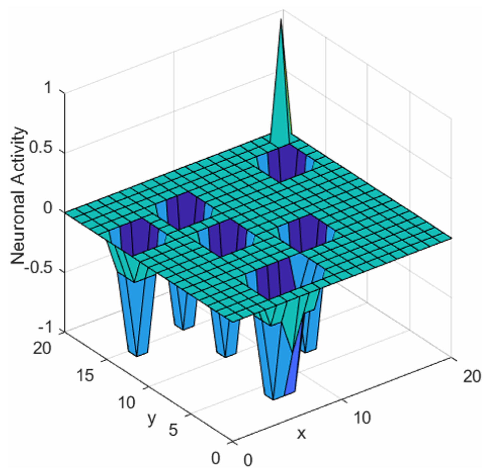
The BINN algorithm regulates neuron activity such that the values for target points reach their peak while those for obstacles drop to their trough, as shown in Figure 4.

3.2. Genetic Algorithm

In the 1970s, John Holland [43], in the United States, proposed the GA, which was inspired by the evolutionary process of organisms in nature. The key to the GA is to simulate the process of natural selection to find the optimal solution to a problem. In the GA, all possible solutions to a problem form a population and each solution is called an individual.
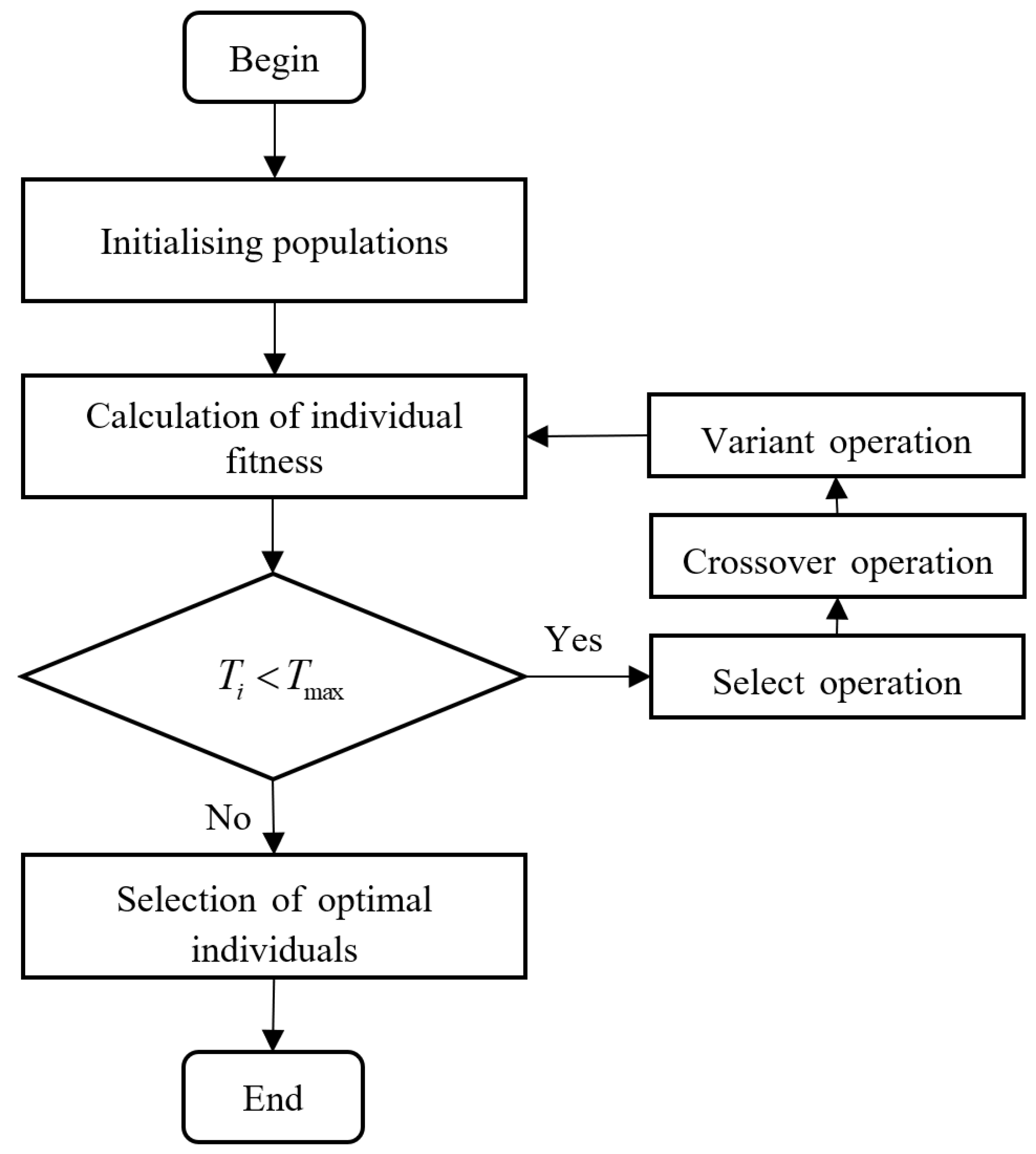
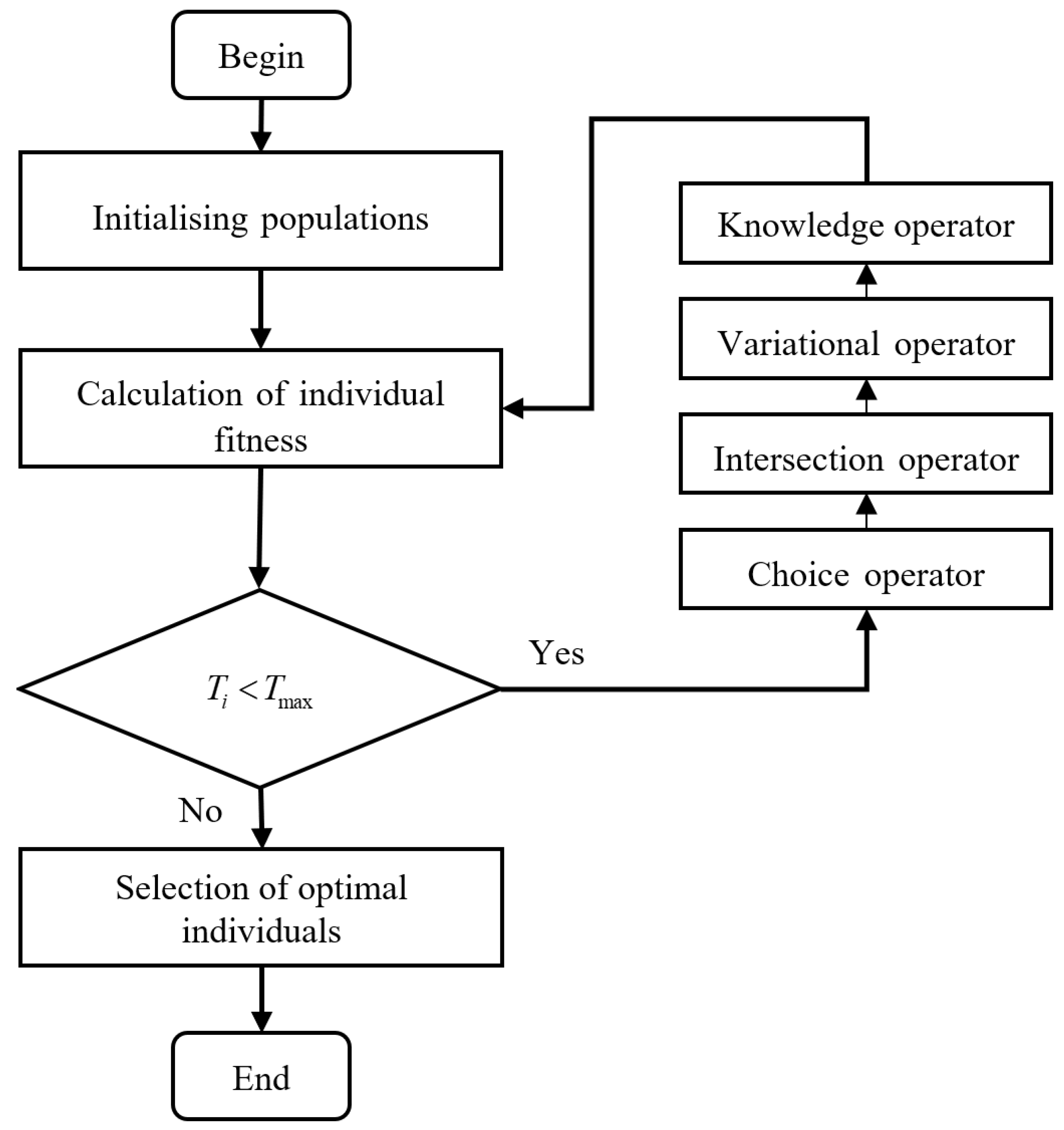
The traditional genetic algorithm consists of operations such as initializing the population, calculating individual fitness values, selection, crossover, and mutation, as shown in Figure 5.
The ultimate goal of robot path planning is to obtain a collision-free shortest path. The path is usually composed of multiple nodes, including the robot start point, destination point, and intermediate nodes, and connecting these nodes is the solved path. The main steps of the GA to solve finding the path are as follows:
Step 1: Initialize the population. Initializing the population involves randomly generating a number of individuals that satisfy the conditions, and each individual in the population is referred to as a chromosome. Multiple initial paths from the start point to the destination point are randomly generated based on the modeling characteristics.
Step 2: Fitness function. The fitness function, also known as the objective function, is a description of the relationship between individuals and fitness, which is a concept used by genetic algorithms to evaluate the optimal value that the population can achieve in the process of evolution. By determining the size of the fitness, the excellent individuals in the population that meet the requirements can be better retained, usually with the shortest path as the goal. The setting of the fitness function is crucial to the entire solution process, which determines the nature of the paths that are eventually solved.
Step 3: Selection operation. Selection is the operation of picking the offspring individuals in the population, through which the individuals with higher fitness in the population are retained and used to perform the crossover operation later. The purpose of this process is to select and retain paths from the population that are more compatible with the solution requirements.
Step 4: Crossover operation. Crossover is an operation that generates a new individual by replacing and recombining parts of the structures of two parent individuals by recombining the genes of two chromosomes to produce a new chromosome that maximizes the inheritance of good traits from the parent chromosome to the next generation of chromosomes.
Step 5: Mutation operation. Mutation is an operation that varies certain gene values of individuals in a population, changing the genes on chromosomes by means of random selection to give the genetic algorithm a local random search capability.

4. The HSBNN Algorithm in This Paper

Aiming at the intelligent path planning problem of mobile robots in complex environments, this paper combines improved BINN and IGA, and proposes an intelligent path planning method based on the HSBNN algorithm for mobile robots in complex road environments. The method mainly uses the activity values of neurons to represent the complex road environment, then establishes a new path-decision model to strengthen the connection between the local path decision and the target point, and finally uses the BINN as the adaptability function of the GA, and uses the IGA to perform the global path planning to achieve intelligent path planning for mobile robots in a complex road environment.

4.1. Genetic Algorithm

In order to solve the problem of traditional neurons having the same activity value at the beginning, this paper relates the magnitude of the neuron’s activity value to the road environment through a mathematical model. The activity value of neuron i in a complex road environment can be expressed by Equation (13):
X i = x i = e S i
Neuron i in a complex road environment receives an external stimulus signal that can be expressed by Equation (14):
I i = E , target E , obstacle E 0 , complex road environments 0 , otherwise
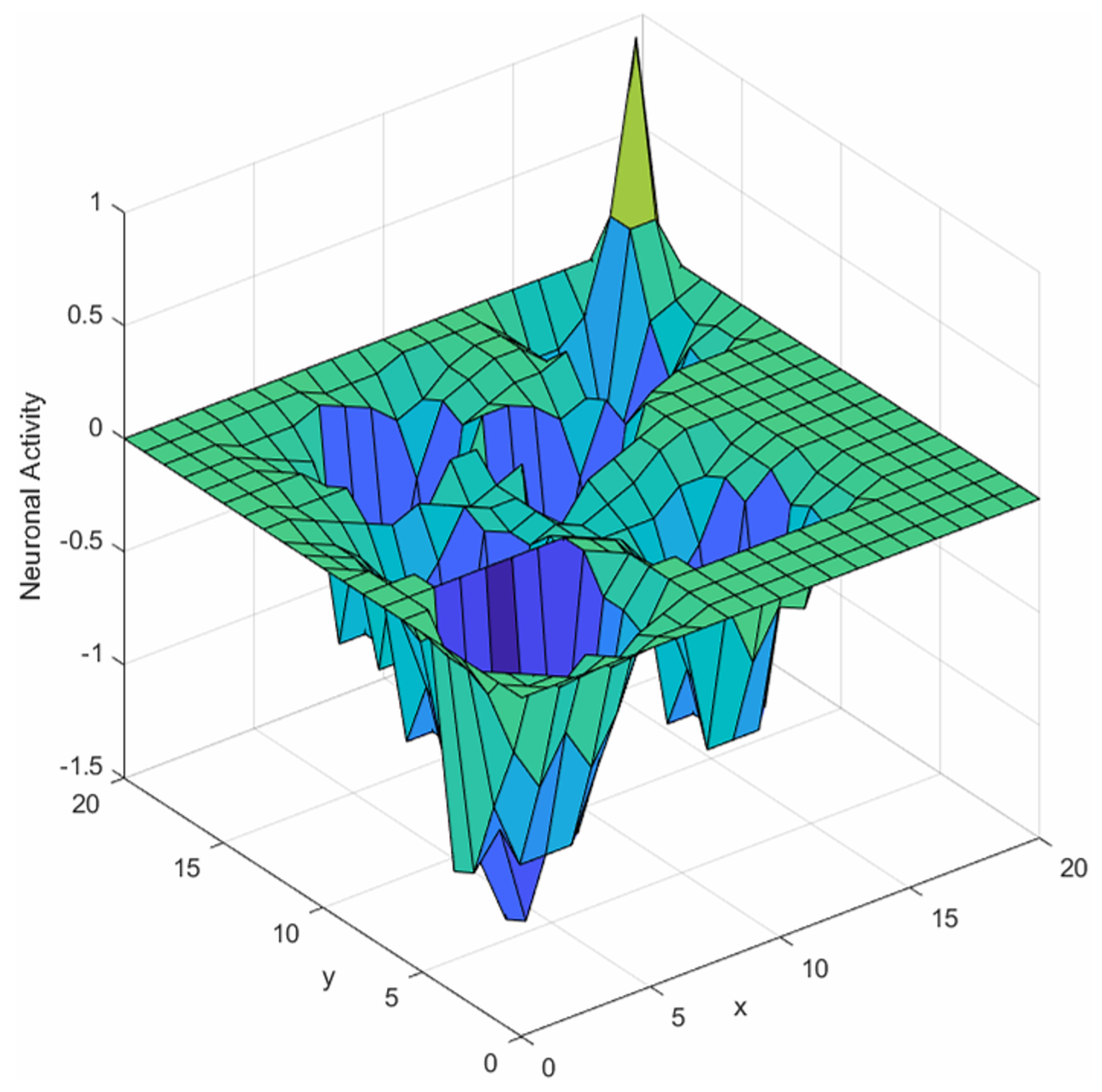
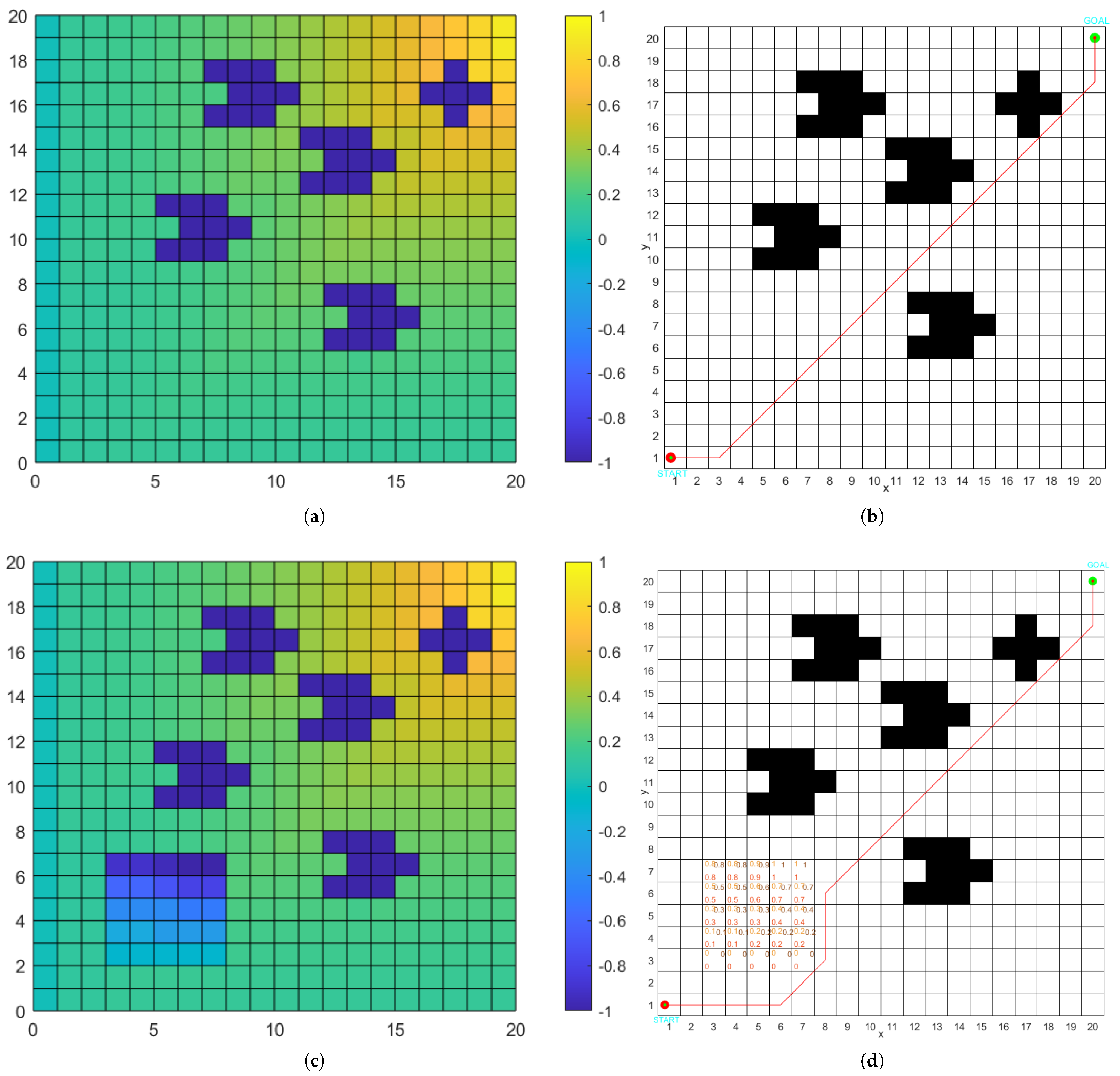
The distribution of initial activity values of neurons in complex environments is plotted in Figure 6.
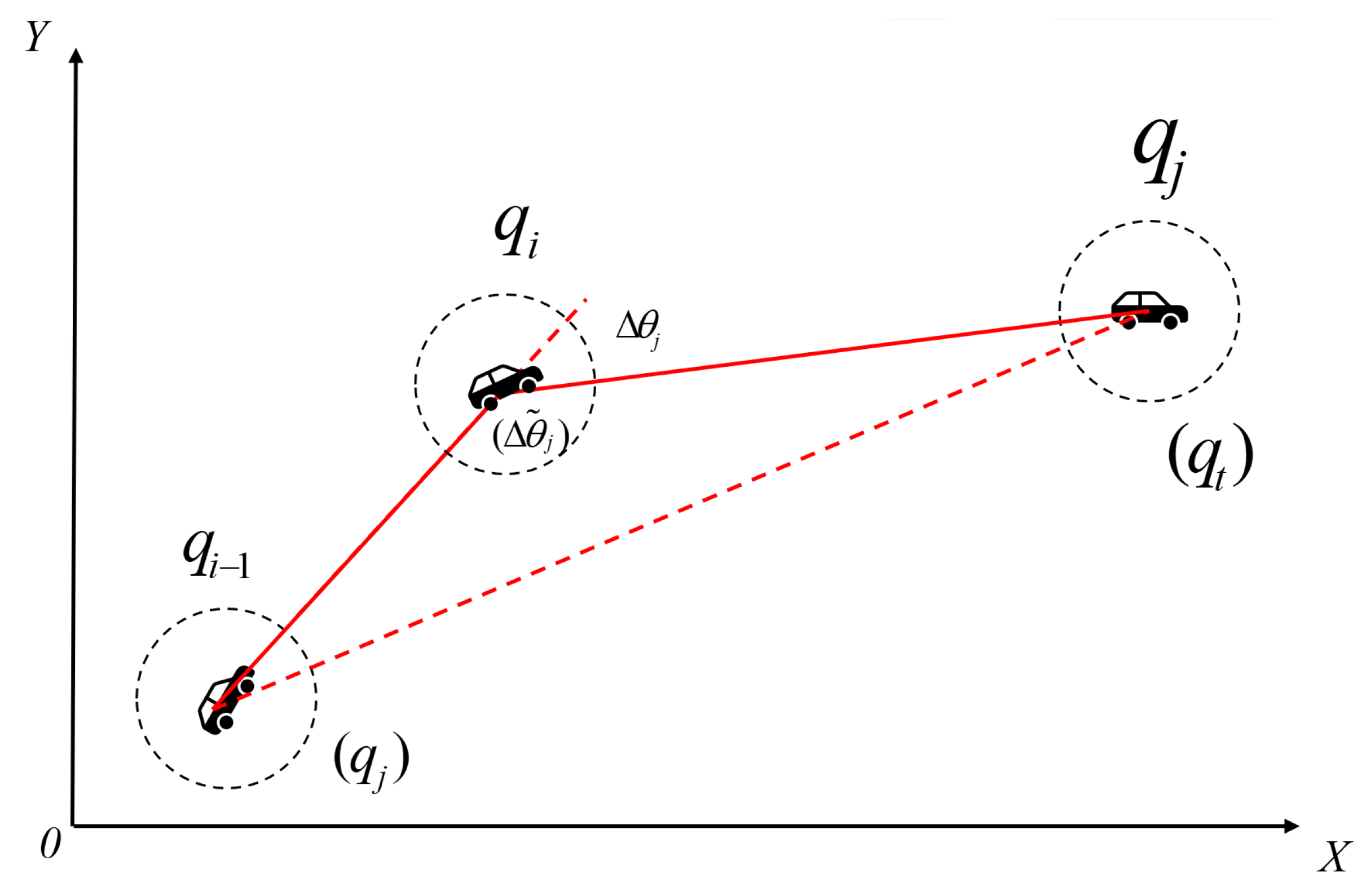
In order to save energy and improve the efficiency of mobile robots, factors such as taking the shortest path and least steering should be considered in path planning. In this paper, the influence of the target point on the path decision is added to the traditional path-decision model, and the next neuron and target-point neuron are introduced to establish a new path-decision model. The association between the local path decision and target point is strengthened by the magnitude of the angle composed of the next neuron, current neuron, and target-point neuron. The new path-decision model is given by Equation (15):
T j = q j = max ( x j + δ 1 y j + δ 2 z j , j = 1 , 2 , , k )
In Equation (15), T j is the path-decision model, q j is the next position, δ 1 and δ 2 are positive constants; y j is the corner function, and z j is the target-point reinforcement function.
The steering function y j is expressed as (16) and (17):
y j = e Δ θ j
Δ θ j = π arccos q i q i 1 2 + q i q j 2 q i 1 q j 2 2 × q i q i 1 2 × q i q j 2
In Equations (16) and (17), Δ θ j [ 0 , π ] is the absolute turning angle of the robot movement.
The motion decision-making method of the robot is shown in Figure 7.
The target reinforcement function z j is expressed as (18) and (19):
z j = cos Δ θ ˜ j
Δ θ ˜ j = arccos q i q j 2 + q i q t 2 q j q t 2 2 × q i q j 2 × q i q t 2
In Equations (18) and (19), q t is the target-point position; Δ θ ˜ j is the angle formed by q j , q i , and q t .

4.2. Improvements to GA

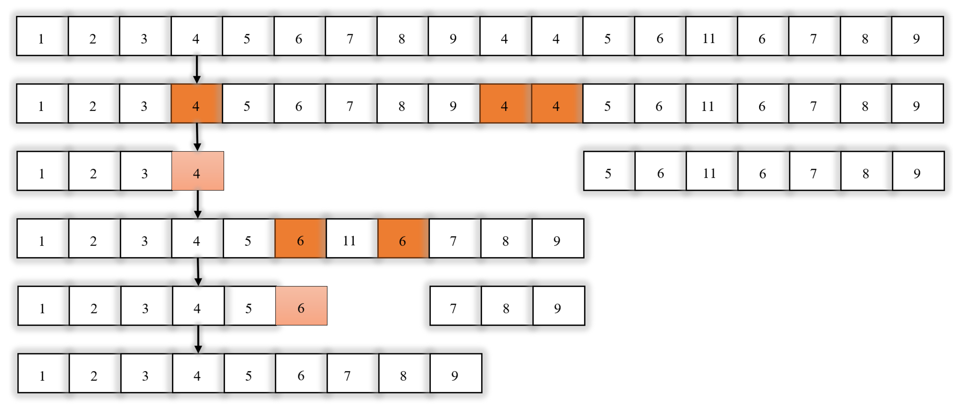
Since genetic algorithms have the same path points after crossover and mutation, the same path points will produce redundant paths, resulting in problems such as increased path length, increased arithmetic, and reduced arithmetic efficiency. To address this problem, this paper proposes a new IGA that adds a new knowledge operator to the traditional genetic algorithm, which removes redundant paths between the same path points in the paths, effectively accelerating the convergence speed, reducing the amount of operation, and improving the optimization efficiency, etc., as shown in Figure 8. The steps of working with the knowledge operator are as follows:
Step 1: Determine if there is an identity for each path;
Step 2: If there is an identity, delete the first to the last point in the identity as well as the last identity;
Step 3: Repeat steps 1 and 2 until all path points are judged.
The workflow of the IGA in this paper is shown in Figure 9.

4.3. HSBNN Algorithm

For the path planning problem for mobile robots, we need to consider the complex road environment factors. The improved BINN algorithm has strong local search optimization ability, but it is insufficient in global optimization ability. In order to improve its global path optimization ability, this paper combines the IGA algorithm with the improved BINN, and proposes the HSBNN algorithm. We take the neuron’s activity value model, path length model, and path-decision model together as the fitness function of the IGA, which can be expressed by Equation (20):
F ( k ) = ω 1 1 L ( k ) + ω 2 1 T ( k ) + ω 3 1 X ( k )
In Equation (20), L ( k ) is the length model of the kth path, T ( k ) is the path-decision model of the kth path, and X ( k ) is the neuron activity value of the kth path. The weights ω 1 , ω 2 , and ω 3 are set at 0.35, 0.35, and 0.3, respectively.
In complex road environments, the length of a path directly affects the energy consumption and operational efficiency of mobile robots. Longer paths result in increased runtime and energy usage, negatively impacting efficiency. Consequently, a weight of 0.35 is assigned to the path length to ensure that the algorithm prioritizes shorter routes during the planning process, thereby enhancing the robot’s operational efficiency.
Path decision making is crucial for ensuring the safety and stability of robots operating in complex environments. Effective path decisions enable robots to navigate around obstacles and challenging terrains, thereby minimizing the risk of collisions and minimizing vibrations during movement. By assigning a weight of 0.35 to path decision making, this highlights its significance in the path planning process, allowing the algorithm to generate routes that are both safer and more stable.
Neuronal activity provides insights into the real-time state of complex road environments, enabling robots to perceive changes in their surroundings and adapt effectively to varying road conditions. For instance, in challenging situations such as potholes or waterlogged surfaces, neuronal activity can assist robots in making more effective decisions. By assigning a weight of 0.3 to neuronal activity, the algorithm can effectively utilize environmental information for path planning while avoiding an over-reliance on any single factor, thus ensuring a balanced integration of multiple considerations in the decision-making process.
L ( k ) can be represented by Equation (21).
L = min i = 1 n 1 x i + 1 x i 2 + y i + 1 y i 2
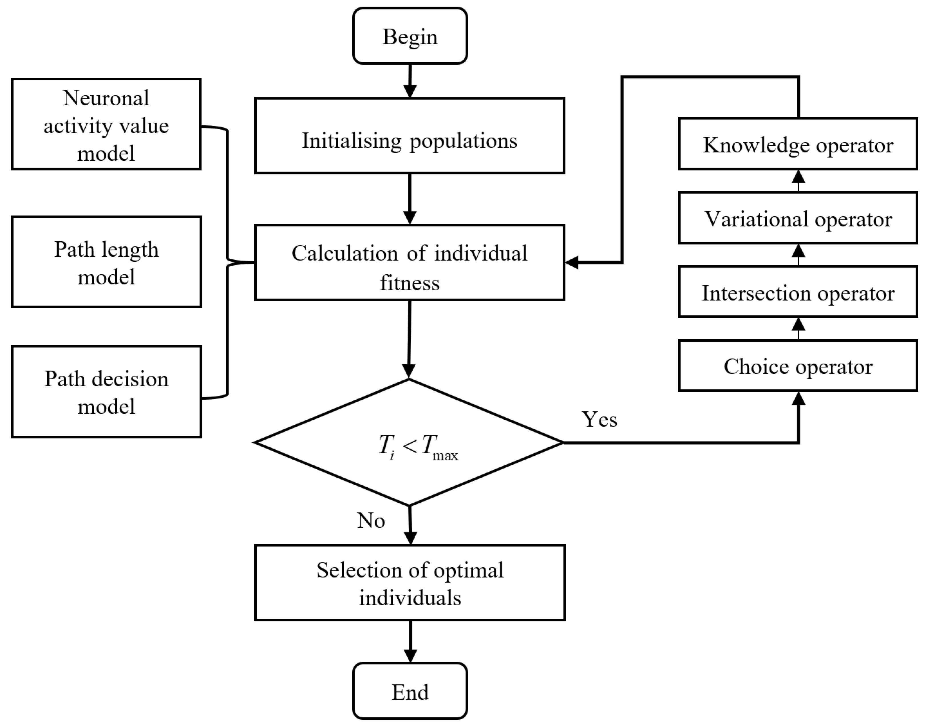
We take the improved BINN as the adaptation function of IGA, and combine the global optimization seeking ability of IGA with the local optimization seeking ability of improved BINN to effectively improve the adaptive ability and work efficiency of mobile robots on complex roads, and the improved HSBNN algorithm is shown in Figure 10.

5. Experiments and Analyses

This study investigates the intelligent path planning capabilities of the HSBNN algorithm in complex road environments. To comprehensively assess the algorithm’s performance and demonstrate its versatility, we conducted experiments along two main lines. The first line of investigation involved performance comparisons, which included three distinct experiments: a comparison of the proposed HSBNN algorithm with existing algorithms, an analysis of grids containing different numbers of obstacles within the same dimensional space, and a comparison of grid maps across various dimensions. The second line examined the algorithm’s adaptability in complex environments through three experiments: evaluating path planning in dynamic scenarios by comparing pre- and post-obstacle movement, assessing the algorithm’s performance without considering road conditions versus in complex road environments, and finally conducting real-world tests with physical robots to validate the algorithm’s performance across various tasks and routes.

5.1. Experimental Configuration

Table 1 presents the experimental configuration for this study.

5.2. Algorithm Performance Experiments

In order to test the algorithmic effectiveness of HSBNN in this paper, and at the same time better reflect the robustness and generality of the algorithm, we performed three different experiments for comparison. The first experiment was to compare and analyze this paper’s HSBNN algorithm with other algorithms; the comparison algorithms are the traditional genetic algorithm (GA), ant colony optimization (ACO), combining BINN and GA (BINN-GA), and the adaptive genetic algorithm (AGA). The second experiment was to compare and analyze different numbers of obstacles in rasters of the same dimensions; the number of obstacles were 20, 50, 80. The third experiment was to compare and analyze raster maps of different dimensions; the raster map dimensions were 10 × 10, 30 × 30, 50 × 50.

5.2.1. Different Algorithms

The experiments in this section were a comparative analysis of HSBNN, GA, AGA, BINN-GA, and ACO. The dimensions of the raster map were 20 × 20 and the number of obstacles was 54.
Genetic algorithm (GA): The computational complexity of GA is primarily determined by the population size, the number of generations in the evolutionary process, and the length of individual encoding. During each iteration, it is essential to compute the fitness function values for all individuals, which involves assessing multiple factors, including path length and decision-making processes. As the population size and the number of evolutionary generations increase, the computational workload grows exponentially. This time complexity is generally represented as O ( N T L ) , where N denotes the population size, T signifies the number of evolutionary generations, and L indicates the length of individual encoding.
Adaptive genetic algorithm (AGA): The AGA introduces a mechanism for the adaptive adjustment of crossover and mutation probabilities based on the principles of the genetic algorithm (GA). While this adaptive mechanism enhances the performance of the algorithm, particularly in terms of convergence speed, it necessitates additional calculations for the adaptive parameters during each iteration, alongside the standard operations of GA. Consequently, the computational complexity is increased compared to GA, resulting in a time complexity represented as O ( N T L + N T ) .
Ant colony optimization (ACO): The computational complexity of ACO is influenced by the number of ants, the number of cities, and the pheromone update strategy. During each iteration, ants traverse paths and update pheromones, yielding a time complexity of approximately O ( m n 2 ) , where m represents the number of ants and n denotes the number of cities. As the scale of the grid map increases, the computational workload increases significantly, leading to an overall rise in complexity.
The main parameters of the algorithm are set as shown in Table 2.
Where T is the number of evolutionary generations, A l p h a is the pheromone importance, R h o is the pheromone evaporation coefficient, and B e t a is the importance of heuristic factors.
Generational evolution (T): In the operation of the genetic algorithm, the algorithm begins with an initial population and iteratively optimizes through processes such as selection, crossover, and mutation, with each iteration referred to as a generation. The generational evolution T determines the total number of iterations during the optimization process. A sufficient number of iterations provides the algorithm with more opportunities to explore the solution space and progressively approach the global optimal solution. If the set generational evolution is too small, the algorithm may fail to fully exploit the solution space, potentially resulting in suboptimal outcomes. Conversely, although a larger generational evolution can theoretically lead to closer approximations of the optimal solution, it may result in increased computational time and resource expenditure.
Population size (N): A population is a collection of multiple individuals, each of which represents a different path in the context of the path planning problem. The population size N indicates the number of individuals participating in the evolutionary operations during each iteration. In this study, N is set to 400. A larger population size enhances the initial solution diversity, thereby increasing the algorithm’s ability to identify the global optimal solution. Since different individuals correspond to various path attempts, a greater number of individuals allows for broader coverage of the solution space. However, if the population size is excessively large, the computational burden may increase significantly, thereby reducing the algorithm’s operational efficiency. Conversely, a population size that is too small may result in insufficient solution diversity, leading the algorithm to converge to a local optimal solution.
Crossover probability ( p c ), maximum crossover probability ( p c _ m a x ), and minimum crossover probability ( p c _ m i n ): The crossover operation is a critical mechanism for generating new individuals in genetic algorithms, achieved by exchanging segments of genes between pairs of parent individuals. The crossover probability ( p c ) determines the proportion of individuals that will undergo crossover operations during each iteration. In this study, pc is set to 0.85, indicating that 85% of individual pairs will participate in crossover operations in each iteration. The parameters p c _ m a x and p c _ m i n are employed in enhanced algorithms, such as adaptive genetic algorithms, to dynamically adjust the crossover probability. When the algorithm exhibits slow convergence, the crossover probability can be increased to improve solution diversity; conversely, as the algorithm nears the optimal solution, the crossover probability can be decreased to prevent disruption of advantageous gene structures. Although this research does not explicitly implement adaptive adjustments, establishing these parameters facilitates potential enhancements to the algorithm.
Mutation probability ( p m ), maximum mutation probability ( p m _ m a x ), and minimum mutation probability ( p m _ m i n ): The mutation operation entails randomly altering certain genes in individual solutions, which introduces new variations into the algorithm and helps prevent premature convergence to local optimal solutions. The mutation probability ( p m ) represents the likelihood of individuals undergoing mutation during each iteration. In this study, pm is set to 0.15, indicating that 15% of individuals may experience mutation in each iteration. The parameters p m _ m a x and p m _ m i n are similarly used for the adaptive adjustment of mutation probability. A mutation probability that is too high may lead to excessive randomness, hindering convergence to a stable solution; conversely, a mutation probability that is too low may prevent effective escape from local optimal solutions, thereby impacting the algorithm’s global search capability.
Importance of pheromone ( A l p h a ), pheromone evaporation coefficient ( R h o ), and importance of heuristic factor ( B e t a ): These parameters are primarily utilized in ant colony algorithms and related methodologies (although this study focuses on the HSBNN algorithm, the comparative analyses involve ant colony algorithms and others). Alpha denotes the significance of a pheromone in the path selection process by ants; a higher alpha value suggests that ants are more likely to choose paths with elevated pheromone concentrations, which can facilitate rapid convergence to effective solutions but may also result in premature convergence to local optima. In this study, the comparison algorithms set alpha = 1, a value that is critical for balancing the influence of pheromone with other factors. Rho represents the pheromone evaporation coefficient, simulating the temporal evaporation of pheromone and controlling the rate of pheromone updates. Rho = 0.25 indicates that after each iteration the pheromone will decrease by a specified proportion, thus preventing excessive accumulation that could trap the algorithm in local optima and ensuring ongoing exploration of new paths. Beta signifies the importance of the heuristic factor, reflecting the degree of dependence ants have on heuristic information (such as distance to the target) when selecting paths. A higher beta value leads ants to prioritize heuristic information, which aids the algorithm in swiftly identifying paths that are near-optimal but may result in the neglect of potentially superior solutions.
Figure 11 illustrates the planning results of the robot across different algorithms.
Based on the optimization search results in Figure 11, we can obtain the data in Table 3.
In Table 3, the comparison of GA, AGA, ACO, BINN-GA, and HSBNN indicates that the HSBNN algorithm yields the best path optimization. The number of turns of HSBNN is 3, which is lower relative to the other algorithms by a maximum of 10 and a minimum of 2 times, significantly reducing the number of turns. The path distance of HSBNN is lower by a maximum of 11.358% compared to the other algorithms, significantly improving the algorithm’s global and local optimization search. Although the time of algorithm operation is not the shortest, it is similar to the operation time of the other algorithms.

5.2.2. Number of Different Obstacles

The experiments in this section were comparative analyses in a 20 × 20 raster map with 20, 50, and 80 obstacles. The optimization search results of HSBNN with a different number of obstacles are shown in Figure 12.
According to the path planning results in Figure 12, we obtain the data in Table 4.
In Table 4, it can be seen that the HSBNN algorithm can find the optimal path with few turns with different numbers of obstacles. In order to make the results avoid chance errors, be more fair and objective, and make the conclusions more convincing, we analyze the distance values of the path planning results of 20 consecutive repetitions by repeating the experiments no less than 20 times, giving the data in Table 5.
In Table 5, we have analyzed the path distance values through 20 experiments and found that the variance and CV(coefficient of variation) change little, while the median and mean are close to each other with little change, demonstrating good stability and generality. Therefore, the HSBNN algorithm can satisfy path finding optimization under different numbers of obstacles.

5.2.3. Raster Maps with Different Dimension Sizes

The experiments in this section are comparative analyses in raster maps of different dimensions; the dimensions of the raster maps are 10 × 10, 30 × 30, and 50 × 50, and the optimization search results of HSBNN in raster maps of different dimensions are shown in Figure 13.
According to the path planning results in Figure 13, we obtain the data in Table 6.
Table 6 shows that the HSBNN algorithm is able to find optimal paths with few turns in raster maps of different dimensions. We analyze the distance values of the path planning results of 20 consecutive repetitions by repeating the experiments no less than 20 times, and we obtain the data in Table 7.
In Table 7, we have analyzed the path distance values through 20 experiments, and found that the variance and CV change little, while the median and mean are close to each other with little change, demonstrating good stability and generality. Therefore, the HSBNN algorithm also has better optimization finding ability and adaptability in maps with different dimensional rasters compared to the other algorithms.

5.3. Experiments in Complex Environments

To assess the adaptability and generality of the HSBNN algorithm in complex environments, we designed three distinct comparative experiments. The first experiment focused on dynamic environments, analyzing path planning variations pre- and post-obstacle movement. The second experiment explored complex road conditions, comparing path planning outcomes both without and with the consideration of detailed road environments. The third experiment involved real-world scenarios, where we evaluated the safety implications of mobile robots navigating different paths tailored to various tasks.

5.3.1. Dynamic Environment

The experiments in this section are conducted in a raster environment of dimensions 20 × 20, and the paths before and after moving the dynamic obstacles are compared, with the number of obstacles set to 50, and the optimization results of the HSBNN in the dynamic obstacle environment are shown in Figure 14.
According to the path planning results in Figure 14, we obtain the data in Table 8.
In Table 8, we can find that the HSBNN algorithm can also find the optimal path in the dynamic environment with few turns. Meanwhile, in Figure 14, we find that the HSBNN is also well adapted in dynamic environments and plans the path dynamically according to the movement of obstacles.

5.3.2. Complex Road Environment

The experiments in this section are carried out in a raster environment of dimensions 20 × 20, and the paths without considering the road environment are compared with the paths in the complex road environment; the number of obstacles is 50, and the optimization search results of HSBNN in a complex road environment are shown in Figure 15.
From Figure 15, we can see that the activity values of neurons are different after considering the complex road environment, and at the same time, it affects the path planning results of the mobile robot. According to the path planning results in Figure 15, we obtain the data in Table 9.
In Table 9, we find that the HSBNN algorithm can also find the optimal path in complex road environments with few turns. Meanwhile, in Figure 15, we find that the HSBNN in this paper also has a very good adaptive ability in complex road environments, and can avoid the uncertainties brought by complex road surfaces, which further improves the adaptive ability of the robot in complex road environments.

5.3.3. Real-World Environment

To further validate the reliability and practicality of the proposed method, we conducted tests using a mobile robot in a real-world setting. Within this environment, we simulated various road conditions, resulting in different paths for the robot depending on the safety tasks executed. The experimental setup was a corridor with dimensions of 12 m by 2.2 m, as shown in Figure 16.
As shown in Figure 16 and Table 10, the paths traversed by mobile robots vary across the four different task safety levels. The analysis shows that the path length increases in correlation with higher task safety levels, validating the capability of mobile robots to plan distinct paths tailored to varying safety requirements.

6. Conclusions

To address the path planning challenges faced by mobile robots in complex road environments, this paper presents the HSBNN algorithm. To enhance the accuracy and effectiveness of the research, we have implemented several innovative improvements: we established a new complex road environment model that comprehensively incorporates factors such as road surface smoothness, adhesion, and gradient, allowing for a more realistic simulation of actual conditions and providing a solid foundation for subsequent path planning. By overcoming traditional limitations, we utilize neuron activation values to represent complex road environments, dynamically linking these values with surrounding road conditions and the robot’s driving status, which significantly enhances the model’s adaptability and flexibility. We developed a new neural network path-decision model that incorporates the influence of target points on path decisions, reinforcing the connection between local path choices and target points. This optimization reduces detours and sharp turns, leading to more efficient path selection. Furthermore, we introduced an improved genetic algorithm that incorporates knowledge-based operators into the traditional framework, effectively eliminating redundant path segments, thereby reducing computational complexity, accelerating convergence speed, and enhancing optimization efficiency.
By integrating the global optimization capabilities of the genetic algorithm with the local optimization strengths of the biologically inspired neural network as the fitness function, we significantly improve the path planning capabilities of mobile robots in complex environments, enabling rapid identification of more optimal paths.
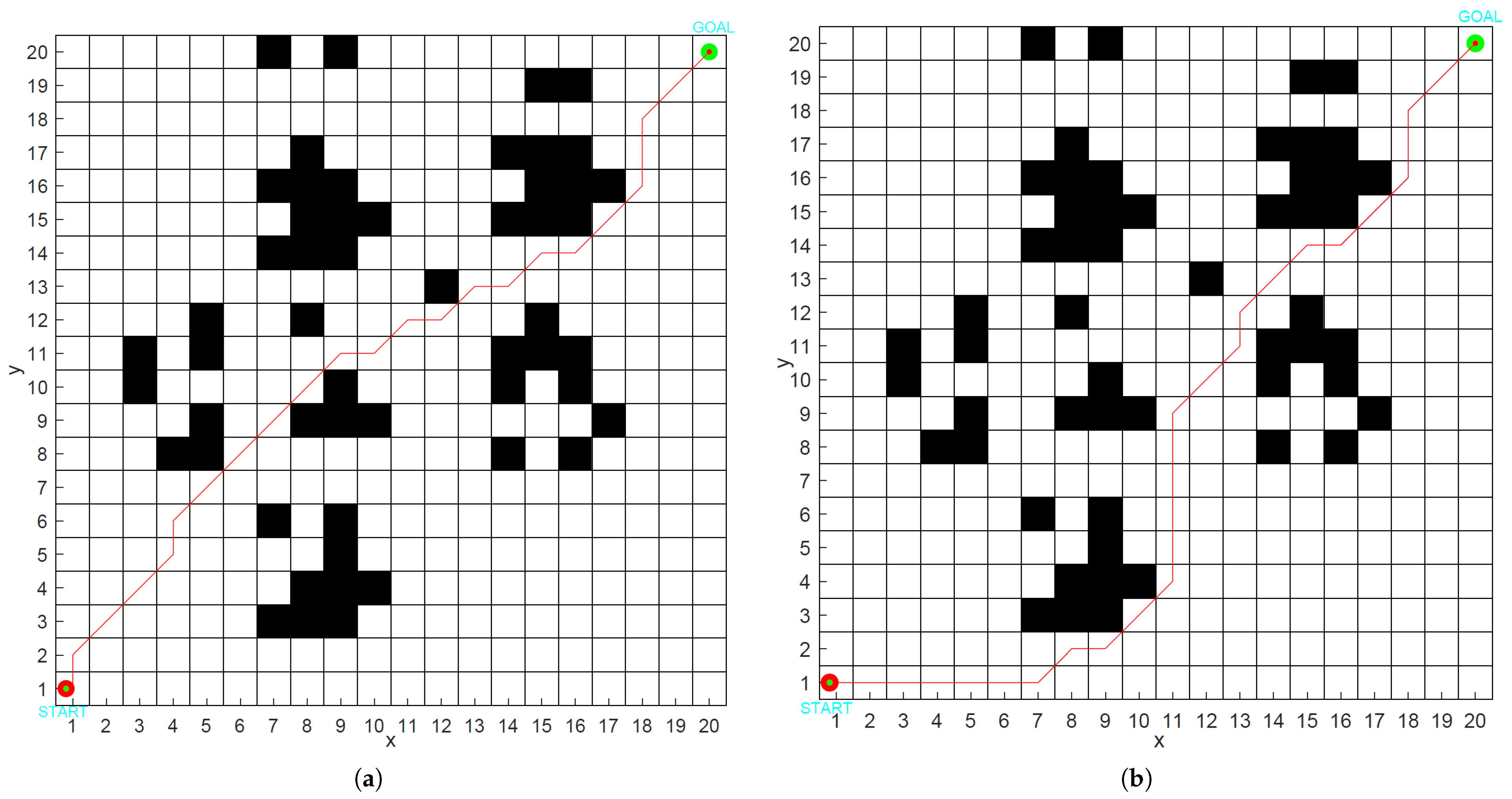
This paper presents a series of experiments conducted across various dimensions, demonstrating that the HSBNN algorithm significantly reduces the number of turns compared to other algorithms, achieving a maximum reduction of 10 turns and a minimum of 2 turns, thereby saving energy during turns. Additionally, the path distance is noticeably shortened, with a maximum reduction of 11.358%, which significantly enhances both the global and local optimization capabilities of the algorithm. In other comparative experiments, we observed that paths planned using the HSBNN algorithm feature fewer turns and shorter distances, effectively illustrating the robustness and universality of the algorithm.
In comparative experiments within complex road environments, we verified that the neuron activation values differ and that these values influence the path planning outcomes for mobile robots. This research can substantially enhance the adaptability and operational efficiency of mobile robots in complex environments. Given the constraints of the study timeline, the experimental validation primarily relies on predefined static environments, with dynamic environment modeling limited to scenarios involving the movement of a single obstacle. The current model’s adaptability to real-time changing complex scenarios and its capacity for real-time updates have not been thoroughly validated, which may compromise the robustness of path planning. Furthermore, the path planning process does not explicitly consider the kinematic constraints of mobile robots. The performance comparison experiments primarily focus on traditional algorithms such as genetic algorithm (GA), adaptive genetic algorithm (AGA), and ant colony optimization (ACO), without contrasting them with recently emerging intelligent algorithms.
To enhance the autonomous adaptability and operational range of mobile robots, we plan to deepen our research in the following directions in the future: 1. Integrate real-time modeling of dynamic environments and online learning algorithms. 2. Incorporate robotic kinematic models to optimize path feasibility. 3. Expand validation efforts to complex scenarios involving multi-robot collaboration and extreme terrain. 4. Design a multi-objective adaptive optimization framework to improve the generalization capability of the algorithms.

Author Contributions

Conceptualization, S.C. and T.F.; funding acquisition, J.L.; investigation, S.C. and T.F.; methodology, S.X.Y., S.C. and T.F.; software, S.C. and T.F.; supervision, J.L. and S.X.Y.; validation, S.C. and T.F.; writing—original draft, S.C. and T.F.; writing—review and editing, J.L. and S.C. All authors have read and agreed to the published version of the manuscript.

Funding

This work was supported in part by the Sichuan Provincial Science and Technology Plan Project (Grant No. 2022NZZJ0036).

Data Availability Statement

The data that support the findings of this study are available from the corresponding author upon reasonable request.

Conflicts of Interest

The authors declare no conflicts of interest.

References

  1. Song, Y.; Tian, W.; Tian, Y.; Liu, X. An efficient calibration method for serial industrial robots based on kinematics decomposition and equivalent systems. Robot. Comput.-Integr. Manuf. 2023, 84, 102607. [Google Scholar] [CrossRef]
  2. Dagnino, G.; Kundrat, D.; Kwok, T.M.; Abdelaziz, M.E.; Chi, W.; Nguyen, A.; Riga, C.; Yang, G.Z. In-vivo validation of a novel robotic platform for endovascular intervention. IEEE Trans. Biomed. Eng. 2022, 70, 1786–1794. [Google Scholar] [CrossRef] [PubMed]
  3. Ren, Q.; Zhu, W.; Cao, J.; Liang, W. Neuro-inspired motion control of a soft myriapod robot. IEEE Trans. Cogn. Dev. Syst. 2023, 16, 606–617. [Google Scholar] [CrossRef]
  4. Del-Rio-Rivera, F.; Ramírez-Rivera, V.M.; Donaire, A.; Ferguson, J. Robust trajectory tracking control for fully actuated marine surface vehicle. IEEE Access 2020, 8, 223897–223904. [Google Scholar] [CrossRef]
  5. Zhou, X.; Wen, X.; Wang, Z.; Gao, Y.; Li, H.; Wang, Q.; Yang, T.; Lu, H.; Cao, Y.; Xu, C.; et al. Swarm of micro flying robots in the wild. Sci. Robot. 2022, 7, eabm5954. [Google Scholar] [CrossRef]
  6. Nian, X.; Li, M.; Wang, H.; Gong, Y.; Xiong, H. Large-scale UAV swarm confrontation based on hierarchical attention actor-critic algorithm. Appl. Intell. 2024, 54, 3279–3294. [Google Scholar] [CrossRef]
  7. Aubin, C.A.; Gorissen, B.; Milana, E.; Buskohl, P.R.; Lazarus, N.; Slipher, G.A.; Keplinger, C.; Bongard, J.; Iida, F.; Lewis, J.A.; et al. Towards enduring autonomous robots via embodied energy. Nature 2022, 602, 393–402. [Google Scholar] [CrossRef]
  8. Patle, B.K.; Pandey, A.; Parhi, D.R.K.; Jagadeesh, A.J.D.T. A review: On path planning strategies for navigation of mobile robot. Def. Technol. 2019, 15, 582–606. [Google Scholar] [CrossRef]
  9. Tang, G.; Tang, C.; Claramunt, C.; Hu, X.; Zhou, P. Geometric A-star algorithm: An improved A-star algorithm for AGV path planning in a port environment. IEEE Access 2021, 9, 59196–59210. [Google Scholar] [CrossRef]
  10. Chen, G.; Liu, D.; Wang, Y.; Jia, Q.; Zhang, X. Path planning method with obstacle avoidance for manipulators in dynamic environment. Int. J. Adv. Robot. Syst. 2018, 15, 1729881418820223. [Google Scholar] [CrossRef]
  11. Luo, Q.; Wang, H.; Zheng, Y.; He, J. Research on path planning of mobile robot based on improved ant colony algorithm. Neural Comput. Appl. 2020, 32, 1555–1566. [Google Scholar] [CrossRef]
  12. Liu, H.; Zhang, L.; Zhao, B.; Tang, J.; Luo, J.; Wang, S. Research on emergency scheduling based on improved genetic algorithm in harvester failure scenarios. Front. Plant Sci. 2024, 15, 1413595. [Google Scholar] [CrossRef]
  13. Lin, S.; Liu, A.; Wang, J.; Kong, X. An improved fault-tolerant cultural-PSO with probability for multi-AGV path planning. Expert Syst. Appl. 2024, 237, 121510. [Google Scholar] [CrossRef]
  14. Mirjalili, S.; Mirjalili, S.M.; Lewis, A. Grey wolf optimizer. Adv. Eng. Softw. 2014, 69, 46–61. [Google Scholar] [CrossRef]
  15. Hou, Y.; Gao, H.; Wang, Z.; Du, C. Improved grey wolf optimization algorithm and application. Sensors 2022, 22, 3810. [Google Scholar] [CrossRef]
  16. Mirjalili, S.; Lewis, A. The whale optimization algorithm. Adv. Eng. Softw. 2016, 95, 51–67. [Google Scholar] [CrossRef]
  17. Wang, W.; Zhang, G.; Da, Q.; Lu, D.; Zhao, Y.; Li, S.; Lang, D. Multiple unmanned aerial vehicle autonomous path planning algorithm based on whale-inspired deep Q-network. Drones 2023, 7, 572. [Google Scholar] [CrossRef]
  18. Mohapatra, S.; Mohapatra, P. American zebra optimization algorithm for global optimization problems. Sci. Rep. 2023, 13, 5211. [Google Scholar] [CrossRef]
  19. Han, L.; Tan, X.; Wu, Q.; Deng, X. An improved algorithm for complete coverage path planning based on biologically inspired neural network. IEEE Trans. Cogn. Dev. Syst. 2023, 15, 1605–1617. [Google Scholar] [CrossRef]
  20. Husbands, P.; Shim, Y.; Garvie, M.; Dewar, A.; Domcsek, N.; Graham, P.; Knight, J.; Nowotny, T.; Philippides, A. Recent advances in evolutionary and bio-inspired adaptive robotics: Exploiting embodied dynamics. Appl. Intell. 2021, 51, 6467–6496. [Google Scholar] [CrossRef]
  21. Rodrigo, D.V.; Sierra-García, J.E.; Santos, M. Glasius bio-inspired neural networks based UV-C disinfection path planning improved by preventive deadlock processing algorithm. Adv. Eng. Softw. 2023, 175, 103330. [Google Scholar] [CrossRef]
  22. Chen, Y.; Liang, J.; Wang, Y.; Pan, Q.; Tan, J.; Mao, J. Autonomous mobile robot path planning in unknown dynamic environments using neural dynamics. Soft Comput. 2020, 24, 13979–13995. [Google Scholar] [CrossRef]
  23. Eftekhari, S.H.; Memariani, M.; Maleki, Z.; Aleali, M.; Kianoush, P.; Shirazy, A.; Shirazi, A.; Pour, A.B. Employing statistical algorithms and clustering techniques to assess lithological facies for identifying optimal reservoir rocks: A case study of the mansouri oilfields, SW Iran. Minerals 2024, 14, 233. [Google Scholar] [CrossRef]
  24. Kianoush, P.; Mohammadi, G.; Hosseini, S.A.; Keshavarz Faraj Khah, N.; Afzal, P. Application of pressure-volume (PV) fractal models in modeling formation pressure and drilling fluid determination in an oilfield of SW Iran. J. Pet. Sci. Technol. 2022, 12, 2–20. [Google Scholar]
  25. Yang, S.X. Real-time robot motion planning and tracking control using a neural dynamics based approach. Dyn. Contin. Discret. Impuls. Syst. Ser. B 2003, 10, 695–708. [Google Scholar]
  26. Yang, S.X.; Meng, M.H. Real-time collision-free motion planning of a mobile robot using a neural dynamics-based approach. IEEE Trans. Neural Netw. 2003, 14, 1541–1552. [Google Scholar] [CrossRef]
  27. Moorthy, S.; Joo, Y.H. Distributed leader-following formation control for multiple nonholonomic mobile robots via bioinspired neurodynamic approach. Neurocomputing 2022, 492, 308–321. [Google Scholar] [CrossRef]
  28. Cai, W.; Zhang, S.; Zhang, M.; Wang, C. Improved BINN-based underwater topography scanning coverage path planning for AUV in Internet of Underwater Things. IEEE Internet Things J. 2023, 10, 18375–18386. [Google Scholar] [CrossRef]
  29. Yao, P.; Wu, K.; Lou, Y. Path planning for multiple unmanned surface vehicles using Glasius bio-inspired neural network with Hungarian algorithm. IEEE Syst. J. 2022, 17, 3906–3917. [Google Scholar] [CrossRef]
  30. Tang, F. Coverage path planning of unmanned surface vehicle based on improved biological inspired neural network. Ocean Eng. 2023, 278, 114354. [Google Scholar] [CrossRef]
  31. Xu, P.F.; Ding, Y.X.; Luo, J.C. Complete coverage path planning of an unmanned surface vehicle based on a complete coverage neural network algorithm. J. Mar. Sci. Eng. 2021, 9, 1163. [Google Scholar] [CrossRef]
  32. Zhu, D.; Tian, C.; Sun, B.; Luo, C. Complete coverage path planning of autonomous underwater vehicle based on GBNN algorithm. J. Intell. Robot. Syst. 2019, 94, 237–249. [Google Scholar] [CrossRef]
  33. Chen, B.; Zhang, H.; Zhang, F.; Liu, Y.; Tan, C.; Yu, H.; Wang, Y. A multirobot distributed collaborative region coverage search algorithm based on Glasius bio-inspired neural network. IEEE Trans. Cogn. Dev. Syst. 2022, 15, 1449–1462. [Google Scholar] [CrossRef]
  34. Yi, X.; Zhu, A.; Li, C.; Yang, S.X. A novel bio-inspired approach with multi-resolution mapping for the path planning of multi-robot system in complex environments. J. Comput. Des. Eng. 2022, 9, 2343–2354. [Google Scholar] [CrossRef]
  35. Li, X.; Li, Q.; Zhang, J. Research on global path planning of unmanned vehicles based on improved ant colony algorithm in the complex road environment. Meas. Control 2022, 55, 945–959. [Google Scholar] [CrossRef]
  36. Hua, C.; Niu, R.; Yu, B.; Zheng, X.; Bai, R.; Zhang, S. A global path planning method for unmanned ground vehicles in off-road environments based on mobility prediction. Machines 2022, 10, 375. [Google Scholar] [CrossRef]
  37. Feng, T.; Li, J.; Jiang, H.; Yang, S.X.; Wang, P.; Teng, Y.; Chen, S.; Fu, Q.; Luo, B. The optimal global path planning of mobile robot based on improved hybrid adaptive genetic algorithm in different tasks and complex road environments. IEEE Access 2024, 12, 18400–18415. [Google Scholar] [CrossRef]
  38. Mnih, V.; Kavukcuoglu, K.; Silver, D.; Rusu, A.A.; Veness, J.; Bellemare, M.G.; Graves, A.; Riedmiller, M.; Fidjeland, A.K.; Ostrovski, G.; et al. Human-level control through deep reinforcement learning. Nature 2015, 518, 529–533. [Google Scholar] [CrossRef]
  39. MA, X.; Zhang, F.; LUO, H.; Gao, F. Evaluation of maturity and moisture content in fresh jujube using fractal theory and tissue images. Food Sci. Technol. 2023, 43, e129922. [Google Scholar] [CrossRef]
  40. Fu, C.; Xu, X.; Zhang, Y.; Lyu, Y.; Xia, Y.; Zhou, Z.; Wu, W. Memory-enhanced deep reinforcement learning for UAV navigation in 3D environment. Neural Comput. Appl. 2022, 34, 14599–14607. [Google Scholar] [CrossRef]
  41. Yin, Y.; Wang, Z.; Zheng, L.; Su, Q.; Guo, Y. Autonomous UAV navigation with adaptive control based on deep reinforcement learning. Electronics 2024, 13, 2432. [Google Scholar] [CrossRef]
  42. Tong, G.; Jiang, N.; Biyue, L.; Xi, Z.; Ya, W.; Wenbo, D. UAV navigation in high dynamic environments: A deep reinforcement learning approach. Chin. J. Aeronaut. 2021, 34, 479–489. [Google Scholar]
  43. Varetto, L. Typogenetics: An artificial genetic system. J. Theor. Biol. 1993, 160, 185–205. [Google Scholar] [CrossRef] [PubMed]
Figure 1. Principles of raster map extension.
Symmetry 17 00836 g001
Figure 2. Principles of raster map extension.
Symmetry 17 00836 g002
Figure 3. BINN mapping relationships in raster maps.
Symmetry 17 00836 g003
Figure 4. BINN activity value. Areas with warm colors correspond to positive values, which indicates a significant influence from the excitation signal of the target point. In contrast, lighter areas or those closer to cool colors correspond to negative values, reflecting the impact of inhibiting signals from obstacles and other factors.
Symmetry 17 00836 g004
Figure 5. The GA principle flowchart.
Symmetry 17 00836 g005
Figure 6. BINN activity values in complex environments. Areas with warm colors correspond to positive values, which indicates a significant influence from the excitation signal of the target point. In contrast, lighter areas or those closer to cool colors correspond to negative values, reflecting the impact of inhibiting signals from obstacles and other factors.
Symmetry 17 00836 g006
Figure 7. Path-decision motion description for mobile robots.
Symmetry 17 00836 g007
Figure 8. Knowledge operator workflow.
Symmetry 17 00836 g008
Figure 9. Flowchart of IGA.
Symmetry 17 00836 g009
Figure 10. HSBNN algorithm.
Symmetry 17 00836 g010
Figure 11. Optimization paths for different algorithms. (a) Results of GA runs. (b) Results of AGA runs. (c) Results of ACO runs. (d) Results of BINN+GA runs. (e) Results of HSBNN runs.
Symmetry 17 00836 g011aSymmetry 17 00836 g011b
Figure 12. Optimization results with different numbers of obstacles. (a) Number of obstacles is 20. (b) Number of obstacles is 50. (c) Number of obstacles is 80.
Symmetry 17 00836 g012
Figure 13. Finding optimal results in raster maps of different dimensions. (a) Raster dimension size of 10 × 10. (b) Raster dimension size of 30 × 30. (c) Raster dimension size of 50 × 50.
Symmetry 17 00836 g013
Figure 14. Path planning results before and after obstacle movement. (a) Path before obstacle movement. (b) Path after obstacle movement. (c) Before and after obstacle movement.
Symmetry 17 00836 g014aSymmetry 17 00836 g014b
Figure 15. Path planning results for complex road environments. (a) Distribution of neuronal activity values at the target point globally when the road environment is not considered. (b) Path planning without considering the road environment. (c) Distribution of neuronal activity values at the target point globally when considering the road environment. (d) Path planning considering complex road environments.
Symmetry 17 00836 g015
Figure 16. Path planning for various safety levels of tasks. (a) Safety level I task. (b) Safety level II task. (c) Safety level III task. (d) Safety level IV task.
Symmetry 17 00836 g016
Table 1. Experimental environment configuration.
HardwareProcessor12th Gen Intel(R) Core (TM) i7-12700H
RAM15.7 GB available
SoftwareOperating systemWindows 11
Table 2. Algorithms’ main parameter settings.
ParameterGAAGABINN-GAACOHSBNN
N40040040010400
T100100100100100
p c 0.85 0.85 0.85
p c _ m a x 0.85
p c _ m i n 0.65
p m 0.15 0.15 0.15
p m _ m a x 0.20
p m _ m i n 0.10
A l p h a
B e t a 7
R h o 0.25
Table 3. Running data of different algorithms.
Algorithm NameNumber of TurnsPath Distance (m)Algorithm Runtime (s)
GA1329.2130.193
AGA1131.5560.198
ACO1029.7992.193
BINN-GA528.0420.266
HSBNN328.0420.326
Table 4. Running data in different quantities.
Number of ObstaclesNumber of TurnsPath Distance (m)Algorithm Runtime (s)
20428.6270.318
50628.0420.323
80828.6270.319
Table 5. Data analysis of 20 repetitions with different numbers of obstacles.
Number of ObstaclesAverage ValueMedianVariance (Statistics)CV
2028.44228.0420.8250.646%
5028.93328.6270.3961.280%
8029.25728.6271.2171.877%
Table 6. Running data in raster maps of different dimensions.
Raster DimensionNumber of TurnsPath Distance (m)Algorithm Runtime (s)
10 × 10313.3140.320
30 × 30342.7700.319
50 × 50571.0540.322
Table 7. Twenty data analyses of raster maps of different dimensions.
Raster DimensionsAverage ValueMedianVariance (Statistics)CV
10 × 1013.41313.3990.2490.554%
30 × 3042.98942.8550.3110.377%
50 × 5071.73671.7260.7641.305%
Table 8. Operational data before and after obstacle movement.
Dynamic EnvironmentNumber of TurnsPath Distance (m)Algorithm Runtime (s)
Pre-movement428.0420.321
After moving628.6270.326
Table 9. Operational data for complex road environments.
Complex Road EnvironmentNumber of TurnsPath Distance (m)Algorithm Runtime (s)
No environmental considerations228.0420.318
Consideration of the road environment429.7990.325
Table 10. Path outcomes for various task safety levels.
Task Safety LevelPath Length (m)
I8.37
II8.74
III9.05
IV9.40
Disclaimer/Publisher’s Note: The statements, opinions and data contained in all publications are solely those of the individual author(s) and contributor(s) and not of MDPI and/or the editor(s). MDPI and/or the editor(s) disclaim responsibility for any injury to people or property resulting from any ideas, methods, instructions or products referred to in the content.

