Abstract
This paper studies a model for competition between natural killer (NK) cells, cytotoxic T lymphocytes (CTLs) and tumor cells, and evaluates the outcomes in the absence and presence of chemotherapy treatment. The growth rate of the tumor is presumed to follow the classical logistic law. The model particularly emphasizes the rate-limiting recruitment of NK cells and CTL cells, which is activated by the presence of the tumor. It additionally includes the activation of CTL cells through debris produced by the lysis of tumor cells by NK cells, alongside the regulatory effect that NK cells have on CTL cells. Additionally, the model incorporates the reciprocal decreases in cell populations resulting from the interactions between tumor cells and immune cells, along with the impact of chemotherapy on all three types of cells. We analyze the stability of the equilibrium points. Utilizing parameter values that have been experimentally confirmed in the literature and applying some elementary principles of singularity theory, we investigate the bistability regimes anticipated by the model in the absence of chemotherapy, and evaluate the impact of model parameters on this behavior. This mathematical analysis serves to evaluate the effectiveness of chemotherapy treatment. We demonstrate that the interplay between the biological parameters in the model and those associated with chemotherapy can result in a range of treatment outcomes. The proposed mathematical analysis may serve as a valuable tool in directing the development of strategies for treatment interventions.
1. Introduction
Cancer is still one of the foremost causes of mortality across the globe. The financial implications of its management and treatment are particularly burdensome for the health care systems in developing countries. In the year 2022, approximately 20 million new cancer cases were reported globally, leading to close to 10 million deaths []. A considerable volume of research is currently aimed at discovering innovative treatments and optimizing the effectiveness of current therapeutic approaches []. Another important domain of research focuses on the application of mathematical models in cancer studies. These models serve as valuable instruments for comprehending complex regulatory processes and can be employed to explore the factors that enhance the immune system’s ability to respond effectively to tumor cells [,].
It is commonly understood that the innate and adaptive immune systems engage with tumor cells by generating unique antigens that are absent in normal cells [,]. In the context of the cell-mediated immune response directed at tumor cells, the key participants are natural killer (NK) cells and CD cytotoxic T lymphocytes (CTLs) [,]. Activating and inhibitory receptors work together to discern target cells, thereby facilitating the activation of natural killer (NK) cells, which represent the primary line of defense for the host body []. Conversely, adaptive immunity is contingent upon CTLs for the identification and destruction of tumor cells [].
The literature presents a variety of modeling approaches that are shaped by the specific immune cell types under consideration, including NK cells, CD T cells, and CD T cells, as well as the required analytical rigor. These methodologies encompass both lumped parameter models, represented by ordinary differential equations (ODEs), and distributed parameter models, described by partial differential equations (PDEs) [,,,,,,,,,,,].
Mathematical models with fractional order have also been proposed to model biological systems [] and tumor–immune interactions []. This modeling approach has the advantages of providing a description of the memory effects which are neglected in classical integer-order mathematical models.
Several of the studies referenced earlier [,,,,,,,,,,,] concerning the mathematical modeling of tumor–immune interactions have focused on examining the occurrences of steady-state multiplicity within these interactions [,,,,,,]. A notable contribution by Kuznetsov et al. [] involved the development of an early model that addressed the existence of multiple equilibria in the dynamics of tumor–immune cell interactions. The model included two specific types of cells: effector cells, which serve as predators, and tumor cells, which are considered the prey. The model predicted the existence of “dormant cells”, characterized by their low concentrations of tumor cells, alongside “active cells”. In addition, it brought attention to coexistence zones where “dormant cells” may elude effector regulation and transition to an active phase [].
Tessi et al. [] formulated a model that encompassed the three critical cell types participating in the tumor eradication process mediated by effector T cells: regulatory T cells, helper T cells, and dendritic T cells. De Pillis and Radunskaya [] subsequently formulated and studied a model concerning tumor and immune cells, which was validated through experimental methods. Their work illustrated the existence of regions of bistability between the disease-free equilibrium and high tumor cell concentration. López et al. [], on the other hand, proposed and investigated a model addressing the interactions between tumor cells and immune cells in the context of chemotherapy, showing strong agreement with experimental results. Their research revealed the existence of bistability between a healthy state and a malignant state, driven by several bifurcation mechanisms, such as saddle-node and transcritical bifurcations. The research conducted by Makhlouf et al. [] focused on the stability of an ODE model that anticipated the interactions among tumor cells, circulating lymphocytes, CD T cells, CD T cells, and natural killer cells, taking into account the impact of chemotherapy. Song et al. [] investigated the stability of a model that outlined linear interactions between tumor cells and immune cells, highlighting the crucial roles played by NK cells and CTLs in the immune surveillance mechanism.
Recently, Bashkirtseva et al. [] expanded upon the system discussed in [] by including the effects of chemotherapy treatment. Their research identified both steady-state multiplicity and periodic behavior within the examined model.
With respect to chemotherapy’s effects, various recent studies (e.g., []) have also analyzed the stability of tumor–immune models that reflect the impact of monoclonal antibody-targeted chemotherapy. This strategy may lead to fewer side effects for patients relative to traditional chemotherapy approaches.
Most of the previously mentioned research employed numerical methods, particularly continuation techniques [], to construct bifurcation diagrams that represent the correlation between the model’s state variables and a designated system parameter. Although these techniques offer certain advantages, they are constrained in their ability to fully depict all branching phenomena that the model can demonstrate. This limitation becomes increasingly evident when the model encompasses a large number of parameters.
The motivation for this study is rooted in the examination of whether a classical model of tumor–immune interactions, augmented by the effects of chemotherapy, can reveal more captivating dynamics than those that have been previously described in the literature [,,,,]. In our mathematical analysis, we apply elementary concepts from singularity theory [,] to study the bistability regimes in the model. At steady state, the model can be condensed into a single function. Consequently, the theory of singularity can serve as a framework for categorizing different branching phenomena within the model. This approach enables the development of practical branch sets that delineate the areas of bistability and aids in analyzing the impact of model parameters on the outcomes of the competition. Additionally, we show that the relative magnitude of the biological parameters in the model, combined with those related to chemotherapy, can lead to a spectrum of treatment outcomes. To our knowledge, this theory has not been previously applied to study models of tumor–immune cell interactions.
The remainder of the paper is organized as follows. Section 2 introduces the model and Section 3 discusses the uniqueness, positivity and boundedness of model solutions. Section 4 investigates the stability of the tumor-free equilibrium. Section 5 focuses on the model in the absence of chemotherapy, and Section 6 addresses the model with chemotherapy. The last section encompasses a discussion.
2. The Model
The proposed model based on the work in [] features interactions between two immune cell types: natural killer (NK) cells and CD T lymphocytes, with a tumor cell population. The equations that define this model are presented in the following:
The variables , , and represent the populations of natural killer cells, cytotoxic T lymphocytes, and tumor cells, respectively. Tumor cells are assumed to grow following a logistic function described by a growth rate of and a carrying capacity of . The impact of NK cells and CTL cells in diminishing tumor cells is represented by and , respectively, where and correspond to the respective proportions of fractional tumor cells that are eliminated by NK cells and CTLs. Furthermore, chemotherapy eliminates tumor cells at a rate of (/mg.day).
The population of NK cells, as described in Equation (2), grows at a rate of , which represents innate immunity, and dies at a rate of . The term denotes the recruitment of natural killer cells that is prompted by the existence of the tumor. In this context, represents the maximum rate of recruitment, while represents the steepness coefficient associated with this recruitment process. Moreover, the presence of tumor cells results in the inactivation of NK cells. This inactivation is represented by , with the parameter denoting the proportion of NK cells that become detached when they interact with tumor cells. Additionally, NK cells are also affected by chemotherapy at a rate of (/mg.day).
For CLT cells (Equation (3)), the parameter indicates the inactivation of CD T cells, which occurs exclusively because of their natural mortality rate, given that it is presumed that CD T cells are absent when tumor cells are not present. The recruitment of CLT cells is represented by the term , where p ( denotes the maximum recruitment rate and is the steepness coefficient associated with recruitment. Some research disregarded this factor [], whereas other studies utilized a more intricate Hill function to illustrate the fractional tumor cell kill [,]. We selected this representation for its straightforwardness and appropriateness. The term corresponds to the stimulation of CD T cells by debris from natural killer lysed tumor cells []. The term refers to the regulatory influence of natural killer cells on CD T cells. It points to the modulation and inhibition of CD T cell activity that occurs when there are abnormally high levels of activated CD T cells, which do not sufficiently respond to the cytokines available in their vicinity []. The inactivation of CD T cells is linked to their engagement with tumor cells, which is represented as at a rate of . Additionally, CD T cells are also affected by chemotherapy at a rate of (/mg.day).
The fourth equation (Equation (4)) describes how the concentration of the chemotherapy drug changes over time, where represents the decay rate of the chemotherapy medication, while u (mg/.day) denotes the daily dose of the drug that is administered to the patient.
The model is rendered dimensionless through the utilization of the following variables:
The dimensionless model becomes:
The model has thus been rendered dimensionless to yield a unity value for both the carrying capacity and the NK source rate. For responses (recruitment rates) of both NK and CD T cells, the dimensionless values and depend on the tumor growth rate . The same goes for dimensionless death rates and of the immune cells. For the terms representing competition between the three types of cells, it can be seen that and depend on the tumor growth rate , while and q depend on both and the carrying capacity . As to the dimensionless steepness coefficients and of recruitment curves of the NK and CD T cells, they both depend on . The rest of the parameters and depend on and/or .
It is known that the values of tumor growth rate and carrying capacity vary not only with the type of tumors but also on their stages of development. Therefore, the analysis of the dimensionless model through variations of its dimensionless parameters around some experimentally validated values is a useful study that can be mapped with a number of tumor cases and stages.
It is also important to highlight that there are connections between the descriptions of such models describing tumor–immune interaction and symmetry concepts. Broadly defined, symmetry signifies the invariance of a particular quantity under various transformations. Accordingly, a notable property of this model is its invariance when certain variable transformations are applied. This model could be transformed into another normalized form for all populations, resulting in transformed variables such as , , , with R being a reference cell number (generally taken to be cells []). The invariance of the equations’ structure can be shown to persist under these transformations.
3. Uniqueness, Non-Negativeness and Boundedness of Solutions
In light of their biological nature, all values of the four state variables are non-negative. This section presents the results pertaining to the uniqueness, positivity and boundedness of the model solutions.
Theorem 1.
Given the initial conditions :
- 1.
- The solutions , and exist and are unique.
- 2.
- The solutions remain non-negative for all .
- 3.
- The solutions are bounded, provided that and .
The proof for Theorem 1 is given in Appendix A. In light of these results, we determine that the model is mathematically well-posed.
4. Analysis of Model Equilibria
At steady state, Equation (8) yields . The tumor-free equilibrium is represented as . The Jacobian matrix is obtained by taking the derivatives of Equations (5)–(9) with respect to ,, and . Calling the right-hand sides of Equations (5)–(9), the elements of the Jacobian matrix are:
When the Jacobian matrix is evaluated at the tumor-free equilibrium, it becomes:
The eigenvalues corresponding to the Jacobian matrix are:
It can be seen that , and are always negative. As for , its sign can be deduced from the analysis of the quadratic equation:
Non-trivial equilibrium points can be derived by determining from the steady state equation of Equation (5),
and solving for from Equation (6),
Substituting Equations (14) and (15) in Equation (7), can be shown to yield a polynomial in of order 13. Among the coefficients of the polynomial, only the leading term is positive. The rest of the coefficients (shown in the Supplementary Materials) can be seen to be either positive or negative. Applying Descartes’ rule shows that the polynomial can have a maximum of 13 positive solutions. However, further analytical manipulation is almost impossible since the expression of coefficients is quite cumbersome, as there is a large number of parameters in the model. The solution of the polynomial and other related equations is carried out numerically using continuation methods of MACONT [], a graphical MATLAB [] package for the interactive bifurcation analysis of dynamical systems.
Throughout the numerical analysis, attention was paid to selecting model parameters to ensure they corresponded effectively to real cases. The selection process was based on the experimental findings detailed in reference []. The values are associated with human clinical trials in which participants diagnosed with metastatic melanoma underwent treatment with carefully selected tumor-reactive T cells []. The following values are selected:
The corresponding dimensionless values are:
5. Bifurcation Analysis in Case of no Chemotherapy
In the absence of chemotherapy, i.e., , the model tumor-free equilibrium is . The eigenvalues of the Jacobian matrix corresponding to this equilibrium state are
Consequently, when , the third eigenvalue consistently remains negative, ensuring that the tumor-free equilibrium is perpetually stable. For , the tumor-free state is always unstable.
The non-trivial equilibria in the case of no chemotherapy () can be shown to be also defined by a polynomial of order 13 in . For this type of equation, the singularity theory defines a number of singularities. We limit ourselves to the hysteresis singularity. The parameter showing the inactivation of NK cells by tumor cells is chosen, for example, as the main bifurcation parameter.
The requirements for the appearance/disappearance of a hysteresis loop are:
Furthermore, several other derivatives must retain non-zero values, specifically , , and .
The hysteresis boundary can be constructed in any parameter space but it is more convenient to show it in the diagram since the equation defines the stability of the tumor-free equilibrium. Figure 1 shows the branch set consisting of the hysteresis boundary (solid line) and the dashed line , for the rest of the model parameters values in Equation (17). The figure is divided into three regions (A), (B) and (C). Region (A) is above the hysteresis curve. Region (B) is above the line and below the hysteresis curve, while region (C) is below the line of hysteresis and below the line . The different behavior expected in these regions is discussed next.
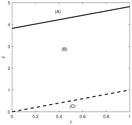
Figure 1.
Branch set in the case of no chemotherapy at the dimensionless parameter values in Equation (17). Hysteresis (solid line) and (dashed line). Region (A) is above the hysteresis curve (solution uniqueness). Region (B) is above the line and below the hysteresis curve, while region (C) is below the line of hysteresis and below the line . Regions (B,C) exhibit some form of bistability.
Figure 2 shows a sample of the bifurcation diagram in region (A) of Figure 1, obtained for . A unique non-trivial steady state exists for all values of and the tumor-free equilibrium is always unstable (since ). Under these conditions, the immune system is unable to suppress the tumor. This is consistent with a system that has a very poor immune response to the cancer.
When crossing the hysteresis line to region (B) of Figure 1, two limit points and are born. The situation is shown in Figure 3, for instance, for . The tumor-free equilibrium is still unstable (since ). There are three branches and the best outcome to hope for is for the system to settle on the low-tumor-cell state. Values of smaller than lead to the low-tumor-cell equilibrium. When is situated between and , the system exhibits bistability. This implies that the external activation of the immune system, which might be perceived as bolstering the immune response (for example, via immunostimulation or changes in initial conditions), can actually prove to be counterproductive, potentially transitioning the system from a low-tumor-cell state to a high-tumor-cell state. Once the second limit point is surpassed, the solutions of the system consistently stabilize at a high concentration of tumor cells. An example of bistability is shown in Figure 4 for . Startup conditions lead the system to settle on the low-tumor-cell conditions, while changes only to initial tumor conditions to lead to the high-tumor-cell conditions.
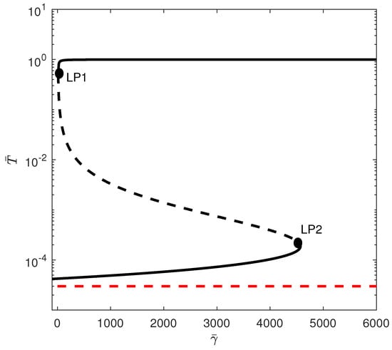
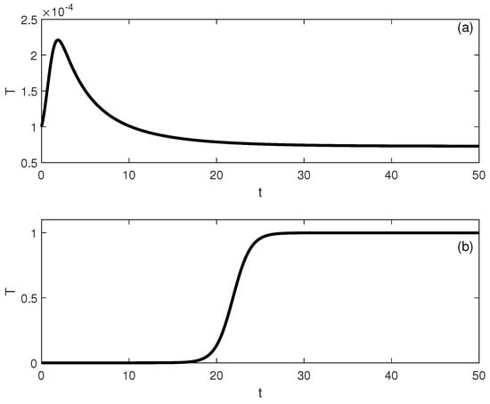
Figure 4.
Time traces showing bisability Figure 3 for . (a) Initial conditions lead to low-tumor-cell conditions, while (b) lead to high-tumor-cell conditions.
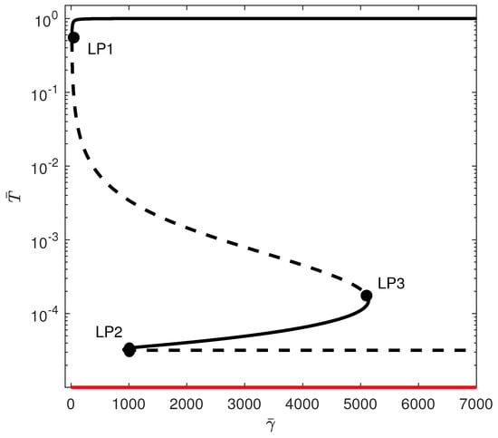
When crossing the line of Figure 1 to region (C), the tumor-free equilibrium becomes stable , but there is the appearance of a third limit point. For some values of , five steady states are possible, of which three are stable. Figure 5 shows an example of the bifurcation diagram for . If is smaller than , then the tumor is completely suppressed as the system settles on the stable tumor-free equilibrium. For values of between and , there is bistability between the tumor-free equilibrium and the high-tumor-cell steady state. For between and , there is coexistence of three stable steady states: the tumor-free equilibrium, the low-tumor-cell state, and a high-tumor-cell steady state. The system may settle on either equilibrium depending on the location of initial conditions relative to the basin of attractions of each equilibrium. For values of larger than , there is bistability between the tumor-free and the high-tumor-cell equilibria.
When the tumor-free equilibrium is stable, the objective of treatment should be to guide the system into the basin of attraction associated with the stable equilibrium of zero tumors.
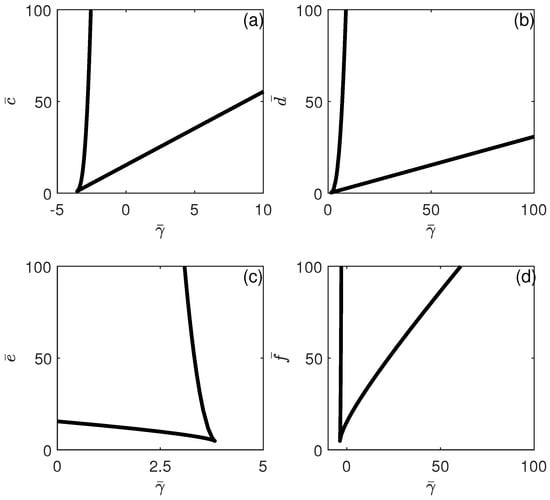
The different behavioral regions depicted in Figure 3 can be charted according to any model parameters. Figure 6 and Figure 7 show the loci of the limit points. Each branch corresponds to a limit point and the hysteresis is expected between the two branches. Figure 5 shows that if any of the parameters , , , or increase, the hysteresis region widens. This suggests that fluctuations in any of these parameters, whether they manifest as increases or decreases, will affect the range of bistability with respect to , either broadening or narrowing it. (Note that the cusp point for the effect of (Figure 6a) occurs for negative values of ). Moreover, while hysteresis is expected for any values of and , hysteresis is expected only for values of and larger than critical values (above the cusp points). Figure 7 shows similar behavior for the effect of and . The effect of shows that bistability in terms of decreases as is increased, and beyond the cusp point, the bistability disappears. This sensitivity analysis shows that all the model parameters have a significant effect on the existence/disappearance of bistability.
6. Bifurcation Analysis in Case of Chemotherapy
When subjected to chemotherapy, the model’s tumor-free steady state has three negative eigenvalues, with the fourth eigenvalue specified by Equations (12) and (13). The quadratic Equations (12) and (13) present the following cases:
- and . In this scenario, both and are positive values. Given that (as indicated in Equation (13)) is consistently negative, the discriminant remains positive at all times. Given that the product of the roots, expressed as , is negative, and their sum, , is positive, it follows that there is a singular positive solution, referred to as , for Equation (12). This implies that the tumor-free equilibrium is stable for all values of exceeding .
- and . In this instance, is a positive quantity and is negative. The discriminant is consistently positive. The product of the roots, expressed as , is negative, and their sum, , is also negative. This situation resembles the previous case, as there is only one positive solution, labeled , to Equation (12), and the tumor-free equilibrium is stable for all values of that are greater than .
- and . In this instance, is negative, and is positive. The discriminant, , can be either positive or negative. When it is positive, there are two positive solutions, and , resulting in an unstable tumor-free equilibrium for values of that lie between and . On the other hand, if the discriminant is negative, the tumor-free equilibrium is always stable.
- and . In this instance, and are both negative. The discriminant can be either positive or negative. If the discriminant is positive, it indicates the absence of positive solutions, and the tumor-free equilibrium is always stable. On the other hand, if the discriminant is negative, the stability of the tumor-free equilibrium is guaranteed.
The condition corresponds to . The hysteresis boundary Equation (19) is also constructed in the parameter space . Figure 8 shows the complete branch set (in logarithmic scale on the y-axis) comprising the hysteresis boundary and the curves and . We can distinguish between four qualitatively different bifurcation diagrams, depicted as , , , and .
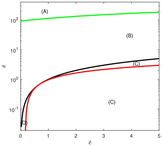
Figure 8.
Branch set in the case of chemotherapy at the dimensionless parameter values in Equation (17). Hysteresis (green), line (black) and (red). Region (A) is located above the hysteresis curve (solution uniquness). Region (B) is located below the hysteresis curve and above the line . Region (C) covers the two domains below the line and also the region below the curve of . Both of these regions (indicated by (C)) yield the same qualitative behavior as far as the disease-free state is concerned. Region (D) is bounded from above by the line and from below by the curve .
Region (A) is located above the hysteresis curve. Region (B) is located below the hysteresis curve and above the line (displayed as the curve in the logarithmic plot). Region (C) covers the domain below the line and also the domain below the curve of . Both of these domains (indicated by (C)) yield the same qualitative behavior, as will be shown next. Region (D) is, on the other hand, bounded from above by the line and from below by the curve .
For the construction of bifurcation diagrams corresponding to the aforementioned regions, it is preferable to designate the intensity of chemotherapy () as the bifurcation parameter. The dimensional values of and (/mg.day) were taken from []. The dimensionless values are and .
The first situation corresponds to region (A). Figure 9 shows the bifurcation diagram obtained, for example, for . For this case, the tumor-free equilibrium is stable beyond a critical point (the only positive solution to the quadratic equation (Equations (12) and (13))). If the chemotherapy drug intensity is increased beyond the critical point, the system solutions stabilize at the tumor-free equilibrium.
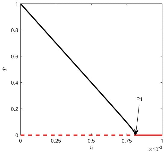
When crossing the hysteresis line into region (B) of Figure 8, two limit points are born. Figure 10 shows an example of the bifurcation diagram for . The tumor-free equilibrium is still stable above a critical point. In this case, values of drug intensity smaller than are unable to suppress the high amounts of tumor cells. For values of between and , there is bistability between the low-tumor-cell and the high-tumor-cell equilibria. Only values of larger than lead to complete suppression of the tumor. Figure 11 illustrates an example of bistability of Figure 10 for . Initial conditions lead to low-tumor-cell conditions, while perturbing to makes the system jump to high-tumor-cell conditions.
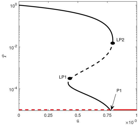
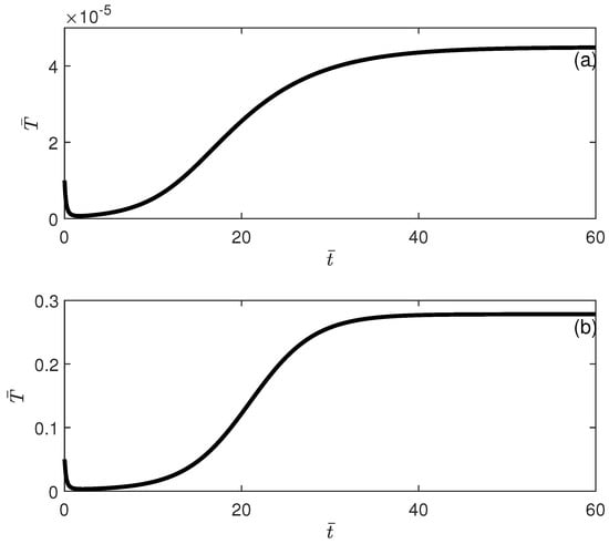
Figure 11.
Time traces showing bisability (Figure 10) for . (a) Initial conditions lead to low-tumor-cell conditions; (b) initial conditions lead to high-tumor-cell conditions.
Region (C) of Figure 8 covers the domain below the line and also the domain below the curve of . In the domain bounded by the line and the curve , the sign of is positive but the two roots are negative. In the domain below , the value of is negative, and therefore, no real root exists. In both cases, the roots are not meaningful, and in the two domains, the tumor-free equilibrium is always stable. Figure 12 shows an example of bifurcation obtained with . A saddle-node bifurcation can be seen. When the intensity of the chemotherapy drug () exceeds the threshold level, the tumor cells are eradicated. Conversely, when the drug intensity falls below this threshold, a bistable state is observed between the tumor-free equilibrium and the elevated presence of tumor cells.
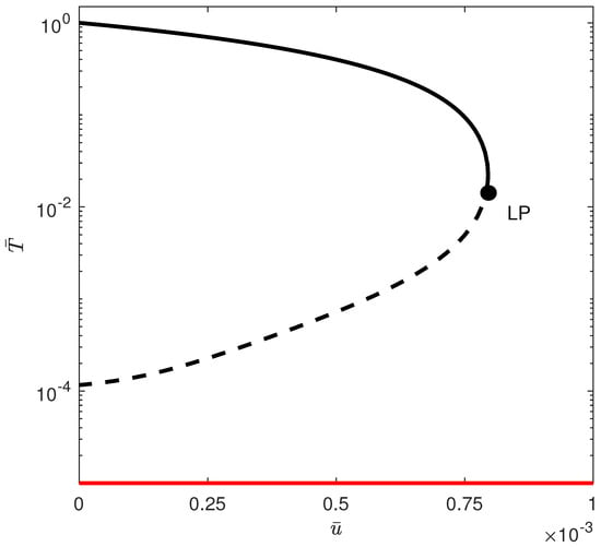
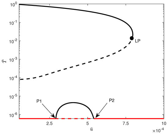
In region (D) of Figure 8, and since there are two positive roots to the quadratic equation (Equation (12)), the tumor-free equilibrium is unstable between the two points and (indicated by arrows) in the bifurcation diagram of Figure 13 obtained with . For drug intensity levels lower than , the tumor-free equilibrium is stable, leading to its coexistence with high tumor cell counts. In the interval between and , the tumor-free state becomes unstable, but there is the appearance of a stable low-tumor-cell state, which coexists with the high-tumor-cell steady state. When the drug intensity exceeds and is below the limit point, the tumor-free equilibrium stabilizes once more, reintroducing a bistability condition with the high-tumor-cell state. Only drug intensity values that are greater than the limit point can fully eliminate the tumor cells.
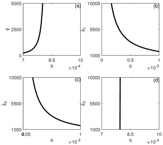
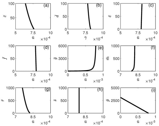
The influence of model parameters on the position of the limit point depicted in Figure 12 is illustrated in Figure 14 and Figure 15. It can be seen from Figure 14 that the limit point is almost insensitive to even large changes in all model parameters except and . An increase in the value of will increase the range of bistability, and therefore, larger drug intensity is needed to completely move the system to stabilize on the tumor-free equilibrium. The effect of an increase in p has the opposite effect, where higher values of would reduce the width of the bistability region. In Figure 15, the impact of chemotherapy-related parameters on the limit point’s location is presented. As predicted, (tumor-associated) decreases with rising values of , while (NK-associated) increases. This implies that greater values of or reduced values of will diminish the amount of chemotherapy required to eliminate the tumor. It is significant to note that the limit point is not influenced by (CTL-associated).
7. Biological Interpretation of Results
Without the influence of immunotherapy or chemotherapy, the model demonstrated the ability to predict bistability, even when subjected to slight alterations in its parameters. In real biological systems, the populations of immune cells and tumor cells are not uniform; instead, they comprise various subpopulations, each characterized by distinct parameter values that govern their behavior. Consequently, fluctuations in these parameter values are highly probable.
Through the application of bifurcation analysis, we were able to attain a profound insight into the dynamics of the system as a whole. Additionally, this analysis successfully highlighted certain parameter values within the model that serve as critical thresholds, beyond which the patient’s system evolves into a stable, tumor-free equilibrium.
When chemotherapy is not being administered, it has been observed that the stability of the tumor-free equilibrium relies entirely on the comparative values of the NK-induced tumor death rate and the NK cell death rate . When the tumor-free steady state exhibits instability , the optimal expectation is to achieve a reduction in tumor size, thereby allowing the system to stabilize at a lower level of tumor cells. However, the phenomenon of bistability could obstruct this desired outcome, as a limited number of tumor cells may successfully evade immune detection, which could drive the system towards a higher concentration of tumor cells.
In scenarios where the tumor-free equilibrium is stable , the system can be sustained at this equilibrium provided that the immune cells are highly effective in eradicating cancer cells. However, for specific model parameters, a state of bistability may emerge between the high tumor cell population and the tumor-free equilibrium, as the immune system’s efficiency diminishes, resulting in the presence of the tumor without its eradication.
The complexity of the tumor microenvironment is considerable, and the phenomenon of immune escape significantly influences tumor development. To achieve a lasting tumor-free condition, any therapeutic approach must not only alleviate the tumor burden but also alter the systemic parameters involved. The aim of therapy design may be to focus on the bifurcation points revealed in our analysis, which is consistent with findings in [,]. In this light, immunotherapy can be regarded as a treatment that changes systemic parameters, particularly by providing a lasting enhancement to the cytolytic function of immune cells []. In addition, adaptive cell transfer can serve to increase the quantity of immune cells, while therapies based on cytotoxic T-lymphocytes (CTLs) can be utilized to improve immune surveillance in the context of developing tumors. Some therapeutic approaches are designed to stimulate the response of cytotoxic T-lymphocytes by linking immune-activating adjuvants, such as viruses or bacteria, to the patient’s own irradiated tumor cells [].
Practical diagrams were also constructed that can help in the design process of model parameters, as to avoid the bistability region altogether or to reduce it. All model parameters (either those associated with NK or CTLs) were found to have a significant effect on the occurrence/disappearance of bistability. This indicates that both natural killer (NK) cells and cytotoxic T lymphocytes (CTLs) are essential components in the immune surveillance of tumors.
The involvement of chemotherapy treatment adds a layer of complexity to the situation.
The model forecasts various scenarios that are solely influenced by the relative importance of the biological parameters of the system, denoted as and , as well as the chemotherapy parameters and , in conjunction with the dose of the administered drug, .
For certain combinations of the previously mentioned parameters, the tumor-free equilibrium remains consistently stable. Bistability between the tumor-free state and a high concentration of tumor cells is dominant, and only values of that exceed the saddle-node critical point will entirely eliminate the tumor.
For other combinations, there exists a critical value of such that any value below this threshold results in an unstable tumor-free equilibrium. This implies that drug levels of that are lower than this critical point cannot effectively inhibit tumor growth. Beyond this threshold, bistability occurs, and the attraction basins can be influenced by the model parameters.
Finally, certain values of the parameters revealed the existence of a middle unstable region in terms of . Bistability with elevated tumor cell levels is observed either above or below this region, while values of that fall between the two critical points lead to the appearance of a low-tumor-cell-concentration steady state and its coexistence with the high-tumor-cell steady state.
It is worth comparing our results to those in the literature. The work in [] showed not only the existence of bistability but also multistability characterized by the coexistence of multiple non-trivial steady states in addition to the disease-free equilibrium. Their results are similar to the ones we obtained, although their model was a simpler two-dimensional model, where the effect of chemotherapy was accounted for by a nonlinear function . The work in [,] used similar models to the one used here, except that a more intricate Hill function was used to describe the fractional tumor cell kills, while the effect of chemotherapy was described by an exponential kill model with a time-delayed concentration, i.e., . Both studies showed that in the absence of chemotherapy, the bistability between the disease-free equilibrium and a malignant state is driven by several bifurcation mechanisms such as saddle-node and transcritical bifurcations. No hysteresis was found, in contrast to our studies. The authors [,] also concurred that therapies like immunotherapeutic vaccines, which alter the parameter values of the dynamical system, offer significant advantages. These therapies have the potential to permanently modify the stability characteristics of the system, thereby reducing the likelihood of disease recurrence. This is the same conclusion reached by our analysis.
8. Conclusions
This research utilized elementary principles of singularity theory to illustrate certain local bifurcation phenomena that can be predicted by a well-known mathematical model representing the interactions between tumor and immune cells. In the absence of chemotherapy, the model predicted bistability in the form of hysteresis across various biological parameters, wherein dormant tumor cells evade immune regulation and transition to an active state.
The analysis also indicated that variations in the intensity of chemotherapy drug are associated with the occurrence of bistability, notably in the form of saddle-node bifurcation and hysteresis.
Within the framework of chemotherapy, we have established that the parameters influencing the emergence of various bifurcation phenomena are, firstly, biological parameters, consisting of the rate at which NK cells induce tumor death and the death rate of NK cells themselves. Secondly, chemotherapy parameters involve the drug’s lethal effect on both the tumor and NK cells, along with the dose of the drug. The remaining model parameters influence these bifurcation behaviors by either enlarging or reducing the areas of bistability, and altering the basins of attraction of the competing attractors.
It was also shown that the complex interplay between the biological parameters of the model and the chemotherapy parameters can lead to a number of scenarios. Certain combinations of these parameters indicated that drug levels falling below a critical threshold are insufficient to suppress the tumor. Conversely, when drug levels exceed this critical threshold, bistability is observed.
Some parameter combinations have shown that, within a certain chemotherapy drug range, the tumor-free equilibrium is invariably unstable and a low-tumor-cell equilibrium appears that coexists with the high-tumor-cell steady state. This situation implies that while small drug doses establish the coexistence of the desired disease-free state with the high-tumor-cell state, increasing the drug dose would form an unfavorable condition where a low tumor cell concentration coexists with a high tumor cell concentration.
Finally, this study was limited to the steady-state behavior. Periodic behavior (Hopf points) was not found in numerical simulations but cannot be ruled out given the large number of parameters. The role of CD T cells could also be added to the model. Moreover, the applicability of these mathematical models goes beyond the comprehension of how biological parameters or chemotherapy influence the occurrence of various bifurcations. Following the identification of these patterns, the next phase is to employ these models to investigate a range of other issues, including the evaluation of the most effective rate of drug administration during patient treatment. This is particularly significant for mitigating the risk of drug toxicity.
Supplementary Materials
The following supporting information can be downloaded at: https://www.mdpi.com/article/10.3390/sym17040492/s1, File S1: Coefficients of the polynomial F(T) of order 13.
Author Contributions
Conceptualization, A.A.; methodology, A.A. and R.T.A.; software, A.A. and R.T.A.; validation, A.A. and R.T.A.; formal analysis, A.A. and R.T.A.; writing—original draft preparation, A.A.; writing—review and editing, A.A. and R.T.A.; funding acquisition, R.T.A. All authors have read and agreed to the published version of the manuscript.
Funding
This work was supported and funded by the Deanship of Scientific Research at Imam Mohammad Ibn Saud Islamic University (IMSIU) (grant number IMSIU-DDRSP2501).
Data Availability Statement
The original contributions presented in the study are included in the article. Further inquires can be directed to the corresponding author.
Conflicts of Interest
The authors declare no conflicts of interest. The funders had no role in the design of the study; in the collection, analyses, or interpretation of data; in the writing of the manuscript; or in the decision to publish the results.
Correction Statement
This article has been republished with a minor correction to the existing affiliation information. This change does not affect the scientific content of the article.
Nomenclature
| c | fractional tumor cells killed by NK cells ( ) |
| d | fractional tumor cell kill by CD T cells () |
| e | death rate of NK cells () |
| f | maximum NK cell recruitment rate by tumor cells () |
| h | steepness coefficient of the NK cell recruitment curve () |
| k | steepness coefficient of the CD T cell recruitment curve () |
| fractional tumor cells killed by chemotherapy () | |
| fractional NK cells killed by chemotherapy () | |
| fractional CD T cells killed by chemotherapy () | |
| m | death rate of CD T cells () |
| p | maximum CD T cell recruitment rate () |
| q | CD T cell inactivation rate by tumor cells ( ) |
| r | rate at which 8 cells are stimulated as a result of tumor killed by NK cells ( ) |
| s | regulatory function by NK cells of CD T cells ( ) |
| u | dose of chemotherapy drug (mg ) |
| C | concentration of chemotherapy drug in blood (mg ) |
| reference value for C (mg ) | |
| L | population of 8 T cells (cells) |
| population of NK cells (cells) | |
| T | population of tumor cells (cells) |
| tumor growth rate () | |
| inverse of tumor carrying capacity () | |
| NK cell inactivation rate by tumor cells ( ) | |
| rate of chemotherapy drug decay () | |
| constant source of NK cells (cells ) | |
| dimensionless variable | |
| static limit point | |
| natural killer cells |
Appendix A
Appendix A.1. Proof of Theorem 1
- Existence and Uniqueness: The right-hand side of the system is continuous and differentiable on and hence locally Lipschitzian []. Therefore, the solution of the model with initial conditions exists and it is unique.
- Positivity: Using the method of variation of constants, for the second model equation (Equation (6)), we haveimplying for provided that .The same can be applied for in Equation (7), while Equation (8) can be solved directly:implying that and for provided that and .For , when , we have , which means hyperplane is invariant, implying for provided that .
- Boundedness: Equation (5) yields:Integration yieldsWe conclude thatFrom Equation (A2), we conclude thatAs for , we have:Using Equation (A5), we have thatThereforeIntegrating yieldsThus, provided that , we haveAs for ,Integrating and using the bounds on (Equations (A5) and (A8)) and Equation (A11) yieldsTherefore, provided that , we have
References
- Bray, F.; Laversanne, M.; Sung, H.; Ferlay, J.; Siegel, R.L.; Soerjomataram, I.; Jemal, A. Global cancer statistics 2022: GLOBOCAN estimates of incidence and mortality worldwide for 36 cancers in 185 countries. CA Cancer J. Clin. 2024, 74, 229. [Google Scholar]
- Pucci, C.; Martinelli, C.; Ciofani, G. Innovative approaches for cancer treatment: Current perspectives and new challenges. Ecancermedicalscience 2019, 13, 961. [Google Scholar] [PubMed]
- Brady, R.; Enderling, H. Mathematical Models of Cancer: When to predict novel therapies, and when not to. Bull. Math. Biol. 2019, 81, 3722. [Google Scholar]
- Rockne, R.C.; Scott, J.G. Introduction to Mathematical Oncology. JCO Clin. Cancer Inform. 2019, 3, 1–4. [Google Scholar] [CrossRef]
- Apavaloaei, A.; Hardy, M.P.; Thibault, P.; Perreault, C. The origin and immune recognition of tumor-specific antigens. Cancers 2020, 12, 2607. [Google Scholar] [CrossRef]
- Jhunjhunwala, S.; Hammer, C.; Delamarre, L. Antigen presentation in cancer: Insights into tumour immunogenicity and immune evasion. Nat. Rev. Cancer 2021, 21, 298. [Google Scholar] [PubMed]
- Stephen, L.; Huntington, N.D. Cytotoxic T Lymphocytes and Natural Killer Cells, in Clinical Immunology, 5th ed.; Rich, R.R., Fleisher, T.A., Shearer, W.T., Schroeder, H.W., Frew, A.J., Weyand, C.M., Eds.; Elsevier: Amsterdam, The Netherlands, 2019; pp. 247–259.e1. [Google Scholar]
- Chiossone, L.; Dumas, P.Y.; Vienne, M.; Vivier, E. Natural killer cells and other innate lymphoid cells in cancer. Nat. Rev. Immunol. 2018, 18, 671. [Google Scholar]
- Coënon, L.; Geindreau, M.; Ghiringhelli, F.; Villalba, M.; Bruchard, M. Natural Killer cells at the frontline in the fight against cancer. Cell Death Dis. 2024, 15, 614. [Google Scholar]
- Hongbo, C.; Pepper, M.; Thomas, P.G. Principles and therapeutic applications of adaptive immunity. Cell 2024, 187, 2052. [Google Scholar]
- Bellomo, N.; Li, N.K.; Maini, P.K. On the foundations of cancer modelling: Selected topics, speculations, and perspectives. Math. Models Methods Appl. Sci. 2008, 18, 646. [Google Scholar]
- Mohammad Mirzaei, N.; Tatarova, Z.; Hao, W.; Changizi, N.; Asadpoure, A.; Zervantonakis, I.K. A PDE model of breast tumor progression in MMTV-PyMT Mice. J. Pers. Med. 2022, 12, 807. [Google Scholar] [CrossRef]
- Ghaffari Laleh, N.; Loeffler, C.M.L.; Grajek, J.; Staňková, K.; Pearson, A.T.; Muti, H.S. Classical mathematical models for prediction of response to chemotherapy and immunotherapy. PLoS Comput. Biol. 2022, 18, e1009822. [Google Scholar] [CrossRef]
- Malinzi, J.; Basita, K.B.; Padidar, S.; Adeola, H.A. Prospect for application of mathematical models in combination cancer treatments. Inform. Med. Unlocked 2023, 23, 100534. [Google Scholar] [CrossRef]
- Kuznetsov, V.; Makalkin, I.; Taylor, M.; Perelson, A. Nonlinear dynamics of immunogenic tumors: Parameter estimation and global bifurcation analysis. Bull. Math. Biol. 1994, 56, 295. [Google Scholar] [CrossRef] [PubMed]
- Robertson-Tessi, M.; Elkareh, A.; Goriely, A. A mathematical model of tumor-immune interactions. J. Theor. Biol. 2012, 294, 56. [Google Scholar] [CrossRef] [PubMed]
- de Pillis, L.G.; Radunskaya, A.E. Modeling tumor-immune dynamics. In Mathematical Models of Tumor-Immune System Dynamics; Eladdadi, A., Kim, P., Mallet, D., Eds.; Springer: Berlin/Heidelberg, Germany, 2014; pp. 59–108. [Google Scholar]
- López, A.G.; Seoane, J.M.; Sanjuán, M.A.F. A validated mathematical model of tumor growth including tumor-host interaction, cell-mediated immune response and chemotherapy. Bull. Math. Biol. 2014, 76, 2884. [Google Scholar] [CrossRef] [PubMed]
- Makhlouf, A.M.; El-Shennawy, L.; Elkaranshawy, H.A. Mathematical modelling for the role of CD4+ T cells in tumor-immune interactions. Comput. Math. Methods Med. 2020, 718, 7602. [Google Scholar] [CrossRef]
- Song, G.; Tian, T.; Zhang, X. A mathematical model of cell-mediated immune response to tumor. Math. Biosci. Eng. 2020, 18, 373. [Google Scholar] [CrossRef]
- Bashkirtseva, I.; Chukhareva, A.; Ryashko, L. Modeling and analysis of nonlinear tumor-immune interaction under chemotherapy and radiotherapy. Math. Meth. Appl. Sci. 2022, 45, 7983. [Google Scholar] [CrossRef]
- Das, A.; Dehingia, K.; Ray, N.; Sarmah, H.K. Stability analysis of a targeted chemotherapy-cancer model. Math. Model Control. 2023, 3, 116. [Google Scholar] [CrossRef]
- Kashif, M.; Singh, M. Existence, uniqueness and Ulam-Hyers stability result for variable order fractional predator-prey system and it’s numerical solution. Appl. Numer. Mat. 2025, 207, 193. [Google Scholar] [CrossRef]
- Feng, X.; Liu, M.; Jiang, Y.; Li, D. Dynamics and stability of a fractional-order tumor-immune interaction model with B-D functional response and immunotherapy. Fractal Fract. 2023, 7, 200. [Google Scholar] [CrossRef]
- Wiggins, S. Introduction to Applied Nonlinear Dynamical Systems and Chaos; Springer: New York, NY, USA, 1990. [Google Scholar]
- Golubitsky, M.; Stewart, I.; Schaeffer, D.G. Singularities and Groups in Bifurcation Theory. Appl. Math. Sci. 1988, 2, 69. [Google Scholar]
- Ajbar, A.; Alhumaizi, K. Dynamics of the Chemostat A Bifurcation Theory Approach; Chapman and Hall/CRC: New York, NY, USA, 2011. [Google Scholar]
- Dhooge, A.; Govaerts, W.; Kuznetsov, Y.A.; Meijer, H.G.E.; Sautois, B. New features of the software MatCont for bifurcation analysis of dynamical systems. Math. Comput. Model. Dyn. Syst. 2008, 14, 147. [Google Scholar]
- MATLAB. Version 9.4.0 (R2018a); The MathWorks Inc.: Natick, MA, USA, 2018. [Google Scholar]
- Dudley, M.E.; Wunderlich, J.R.; Robbins, P.F.; Yang, J.C.; Hwu, P.; Schwartzentruber, D.J. Cancer regression and autoimmunity in patients after clonal repopulation with antitumor lymphocytes. Science 2002, 298, 850. [Google Scholar] [CrossRef]
- Hirsch, M.W.; Smale, S.; Devaney, R.L. Differential Equations, Dynamical Systems, and an Introduction to Chaos; Academic Press: Cambridge, MA, USA, 2012. [Google Scholar]
Disclaimer/Publisher’s Note: The statements, opinions and data contained in all publications are solely those of the individual author(s) and contributor(s) and not of MDPI and/or the editor(s). MDPI and/or the editor(s) disclaim responsibility for any injury to people or property resulting from any ideas, methods, instructions or products referred to in the content. |
© 2025 by the authors. Licensee MDPI, Basel, Switzerland. This article is an open access article distributed under the terms and conditions of the Creative Commons Attribution (CC BY) license (https://creativecommons.org/licenses/by/4.0/).
