
Dynamic Responseof Complex Defect near Anisotropic Bi-Material Interface by Incident Out-Plane Wave


Abstract
1. Introduction
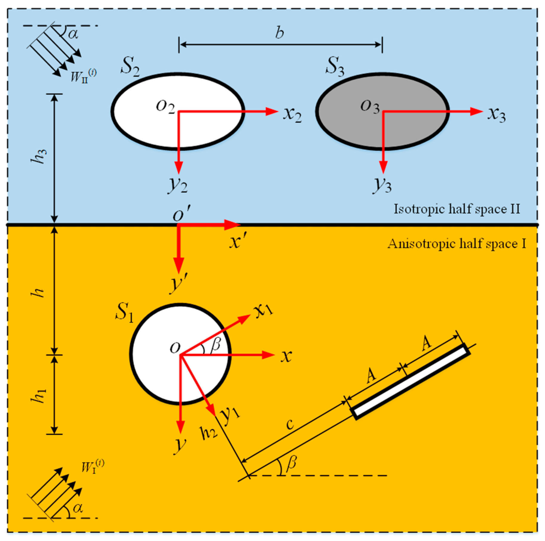
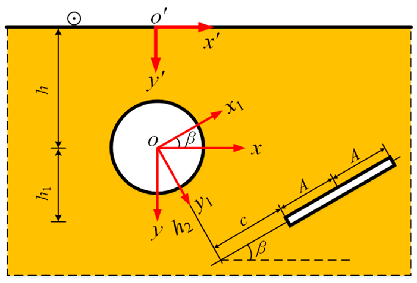
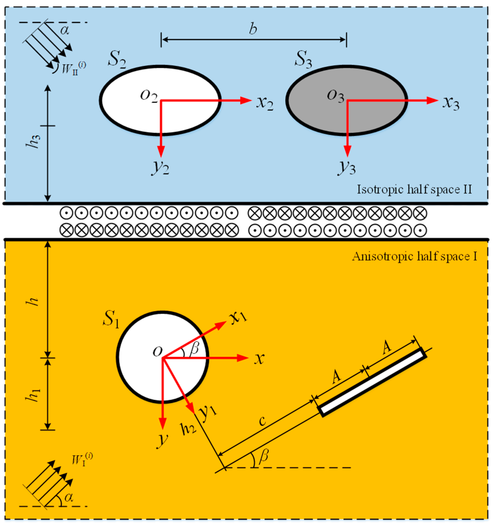
2. Analytical Model
3. Governing Equation
4. The Scattering Waves Around the Cavities and the Inclusion
4.1. The Scattering Wave Around the Circular Cavity in Medium I
4.2. The Standing Wave in Medium III
5. Green’s Function
5.1. Green’s Function G1
5.2. Green’s Function G2
5.3. Green’s Function G3
5.4. Green’s FunctionG4
6. Plane SH Wave Incidence in Two Half Spaces
6.1. Wave Fields in Anisotropic Half Space
6.2. Wave Fields in Isotropic Half Space
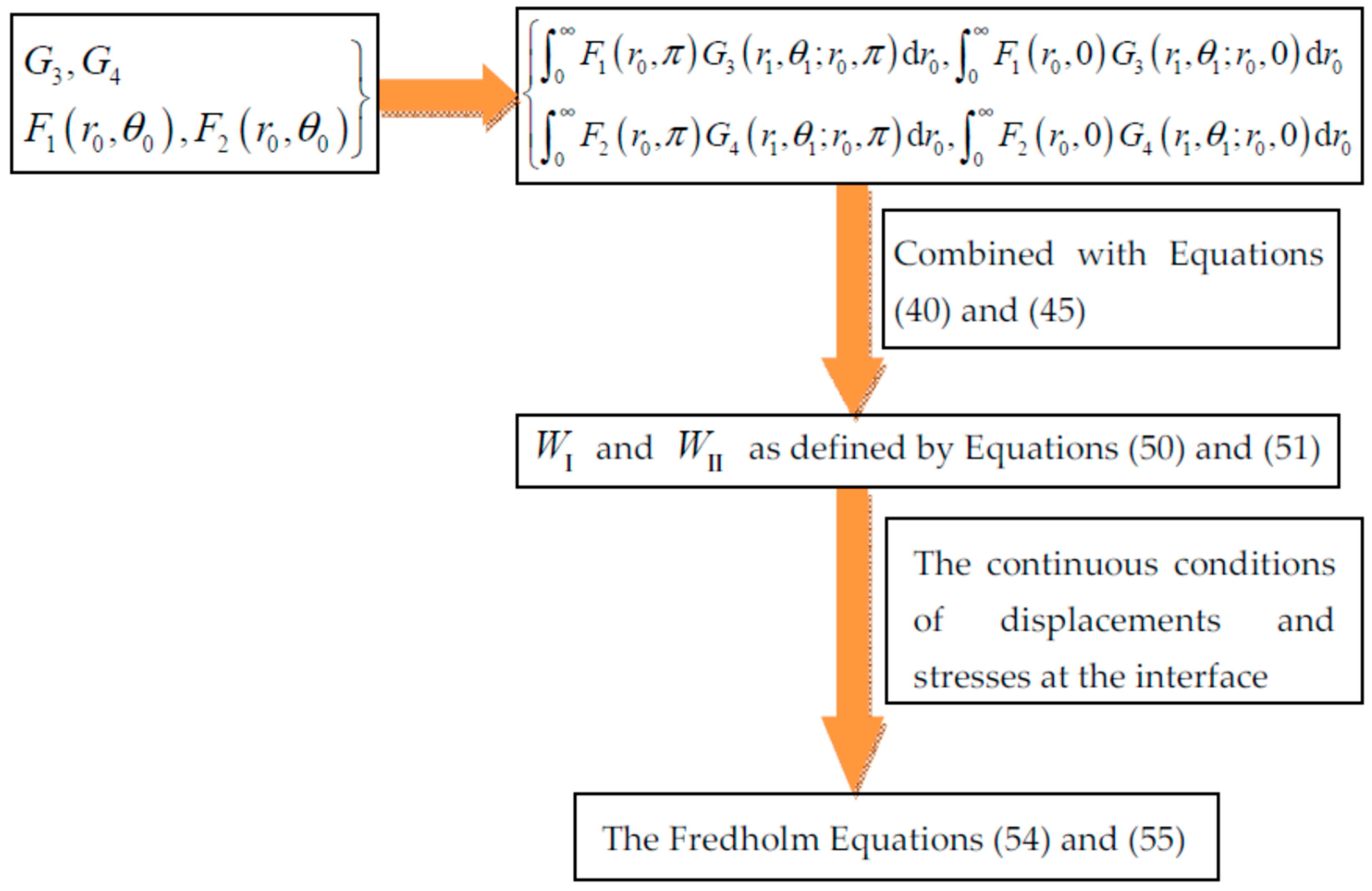
7. Definite Integral Equations
8. Dynamic Stress Concentration Factor (DSCF) at the Cavity
9. Numerical Results and Discussion
10. Discussion and Conclusions
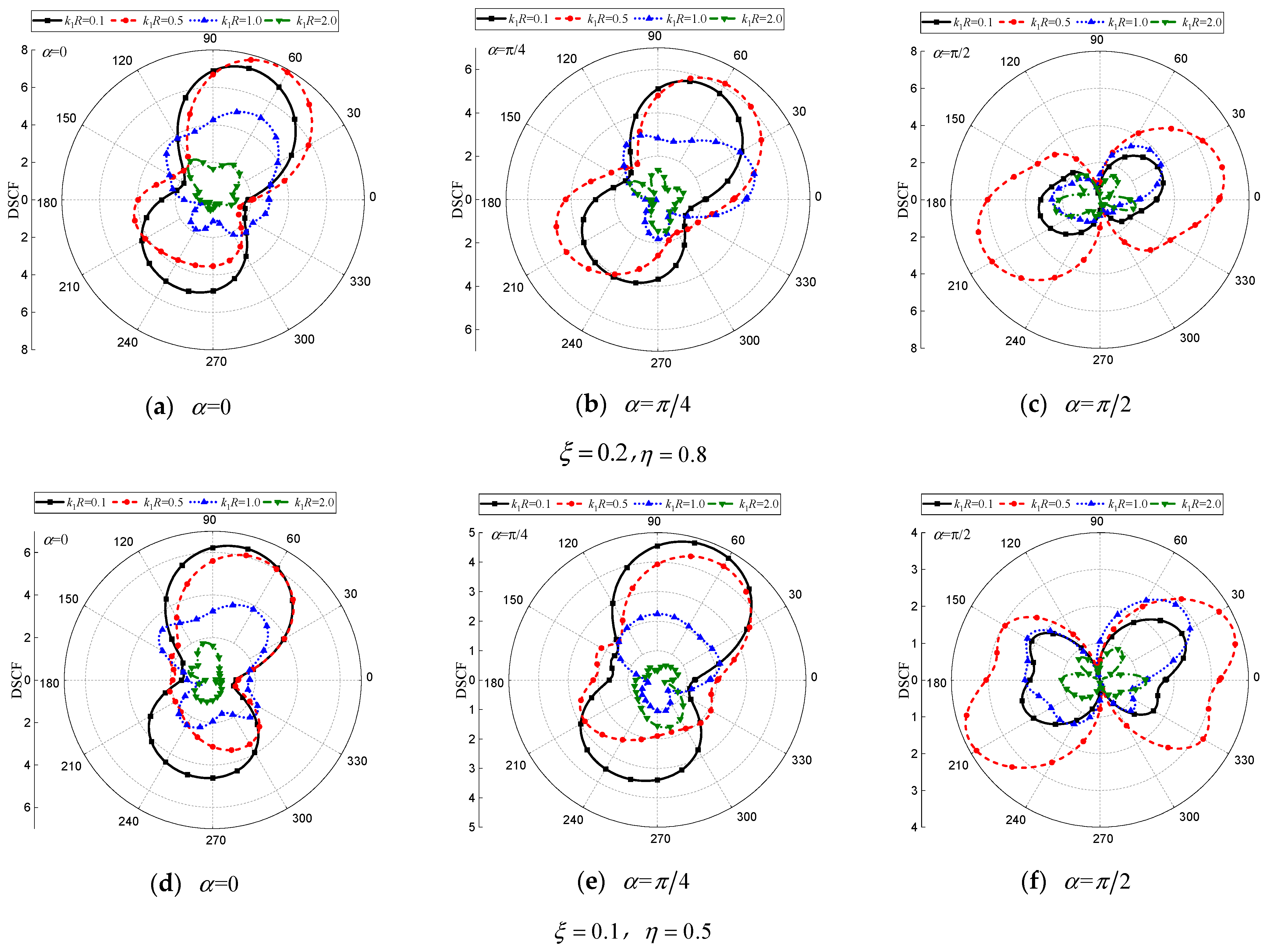
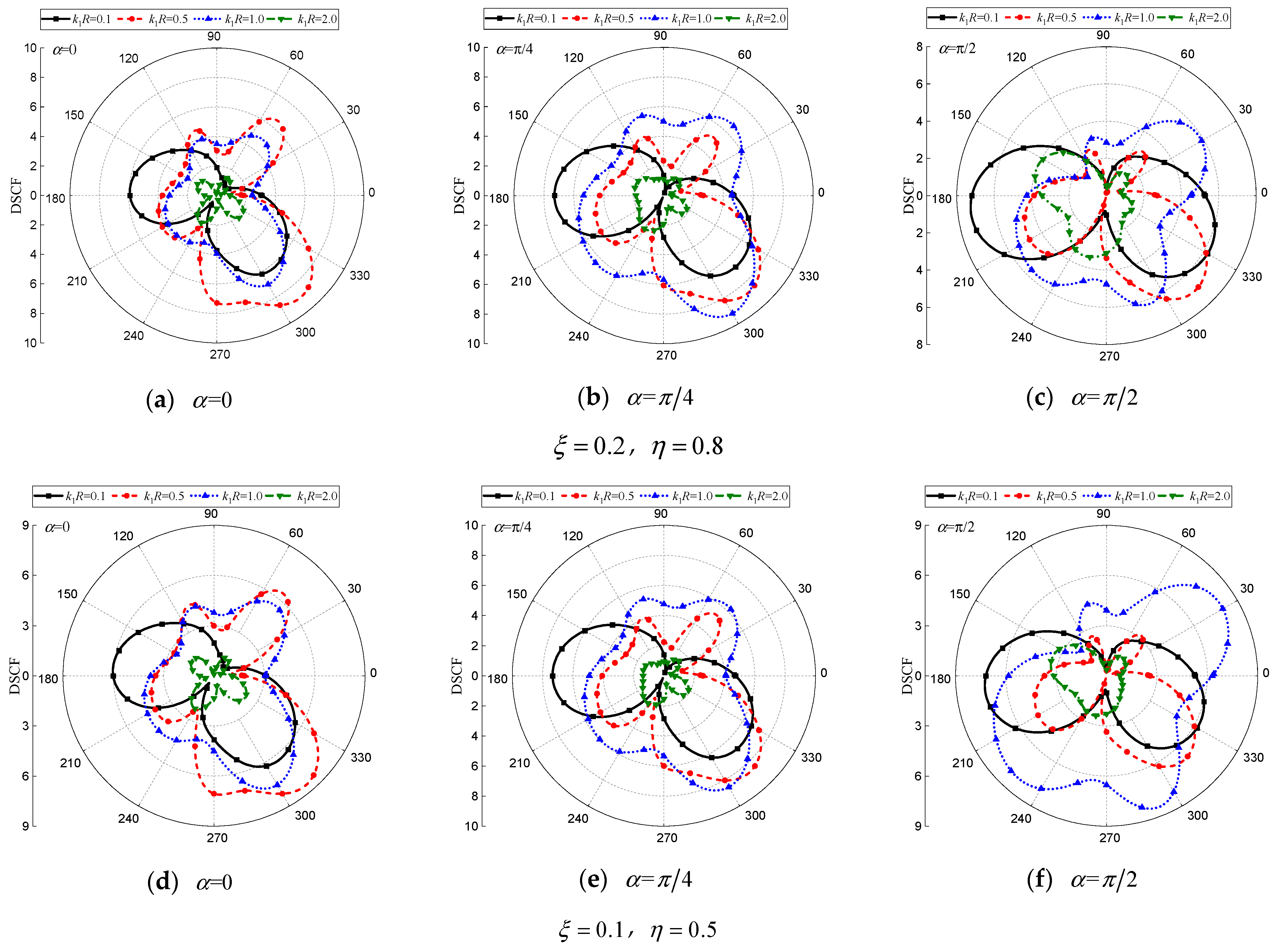
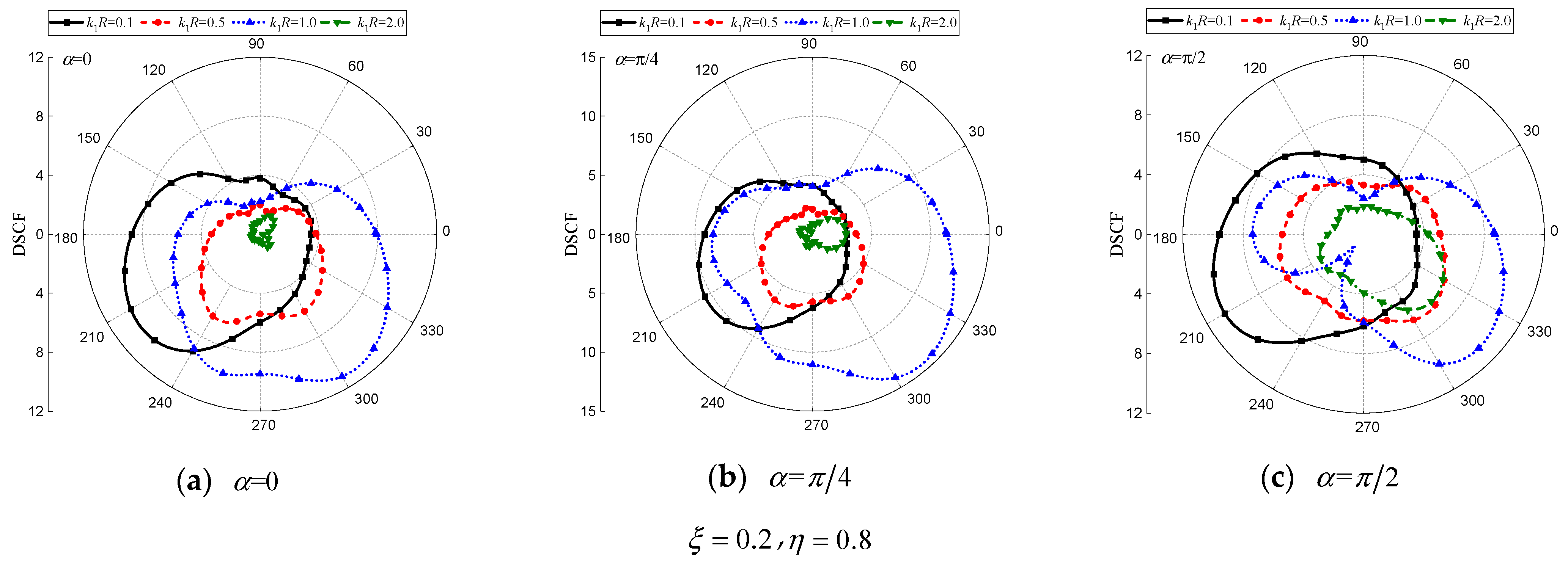
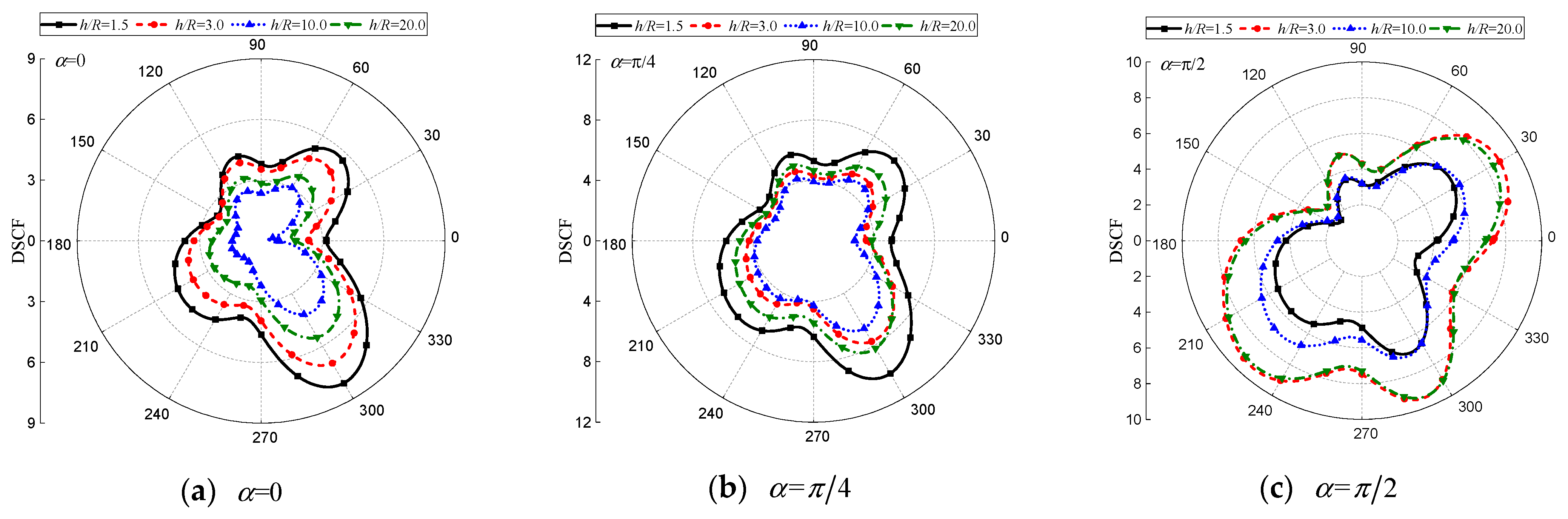
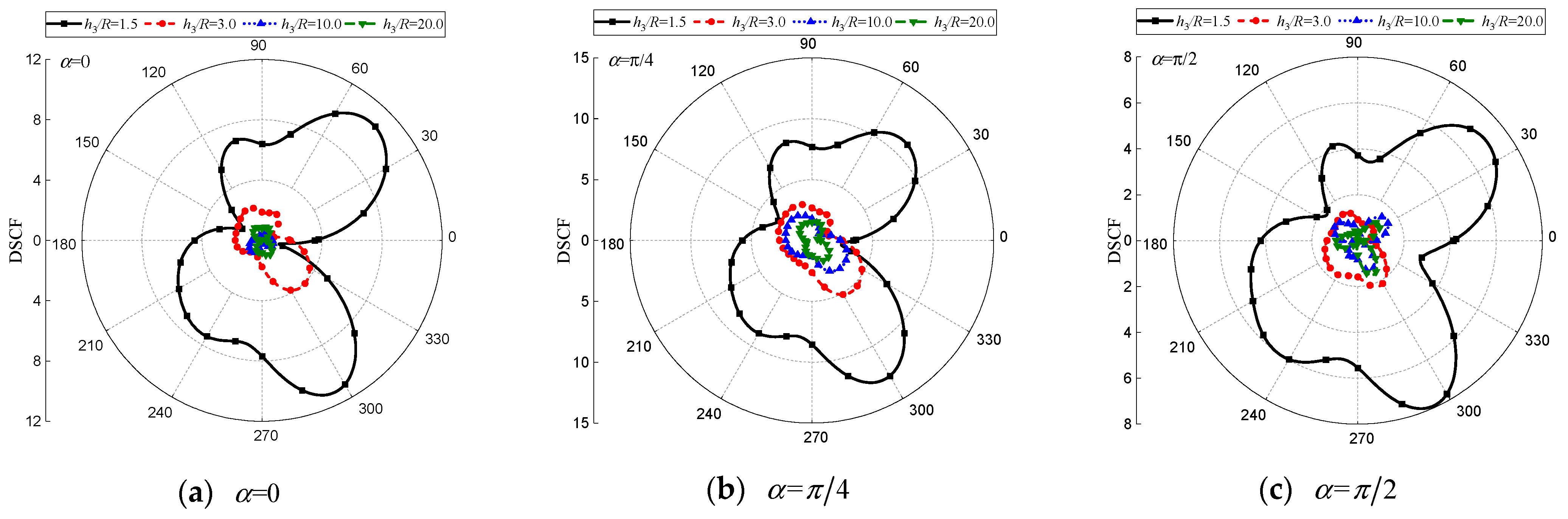
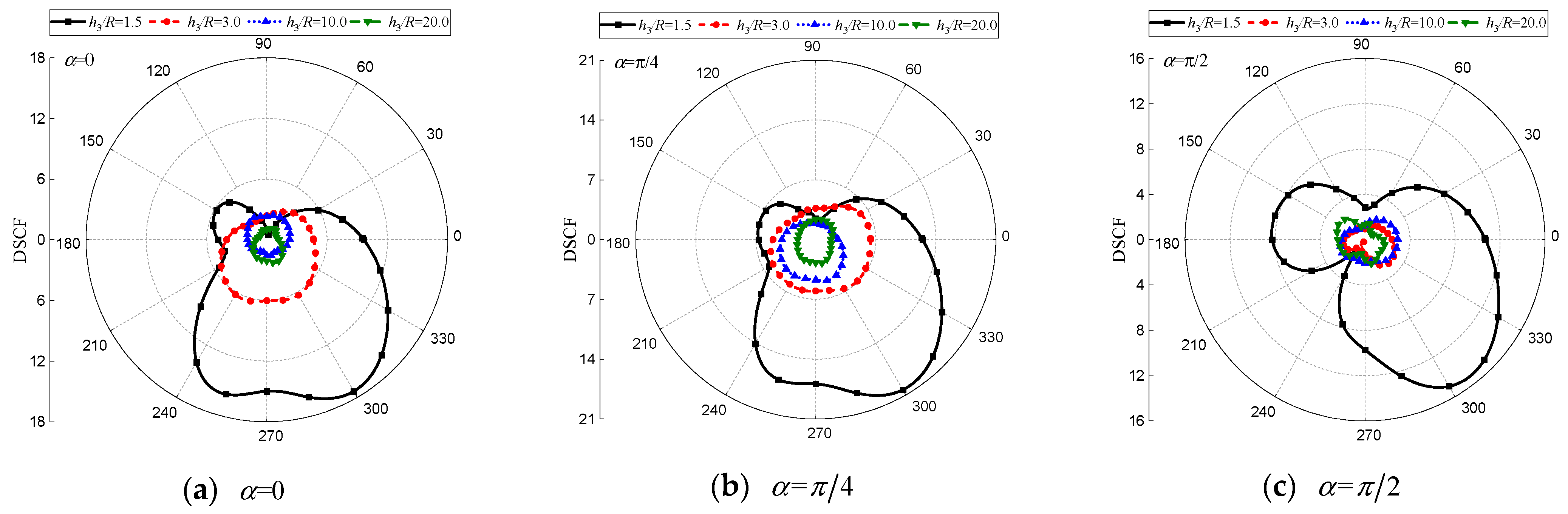
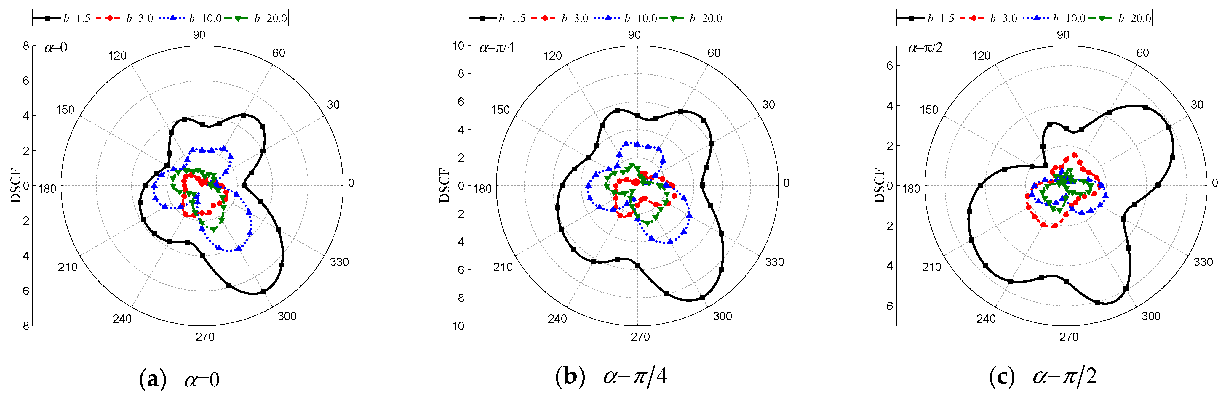
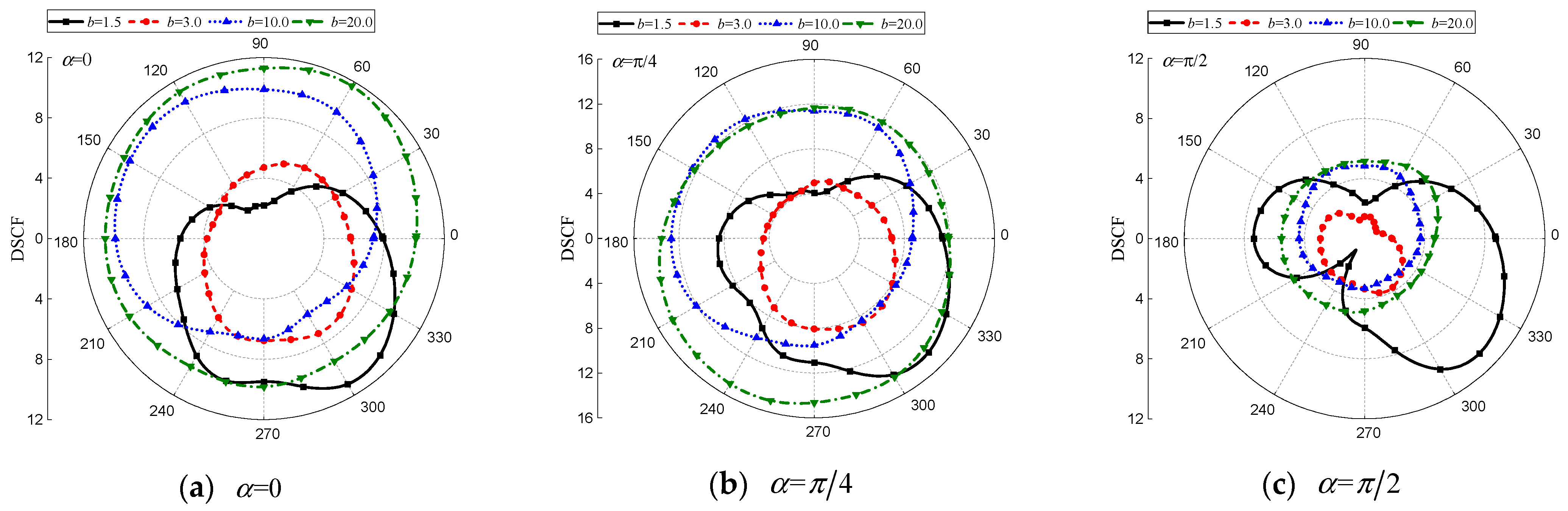
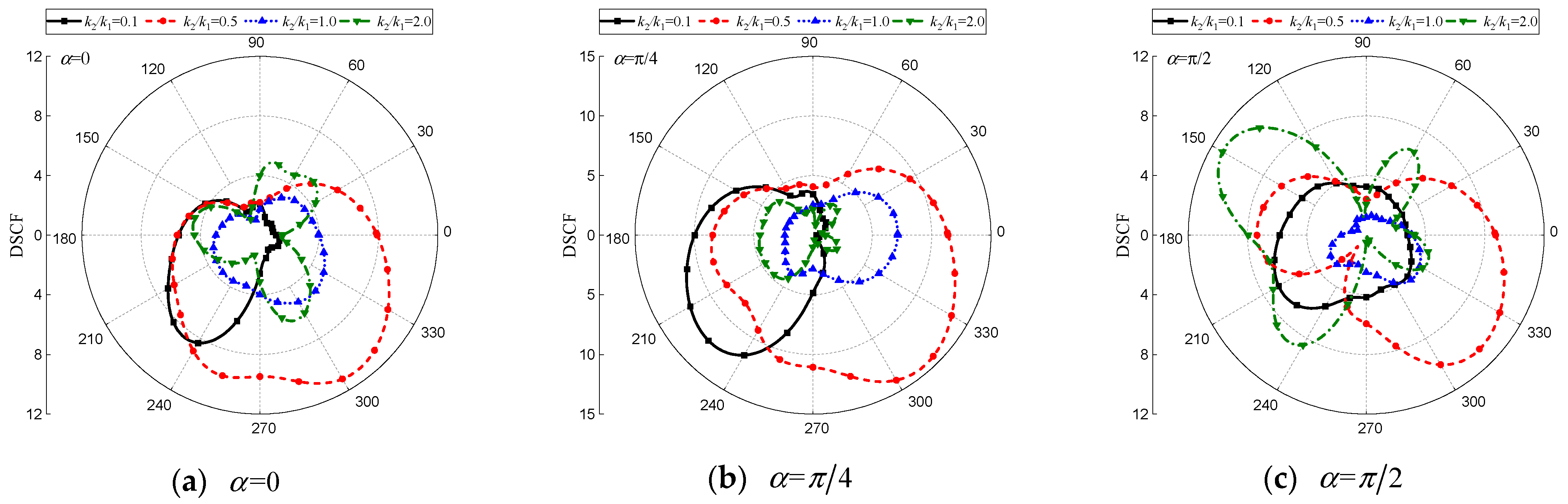
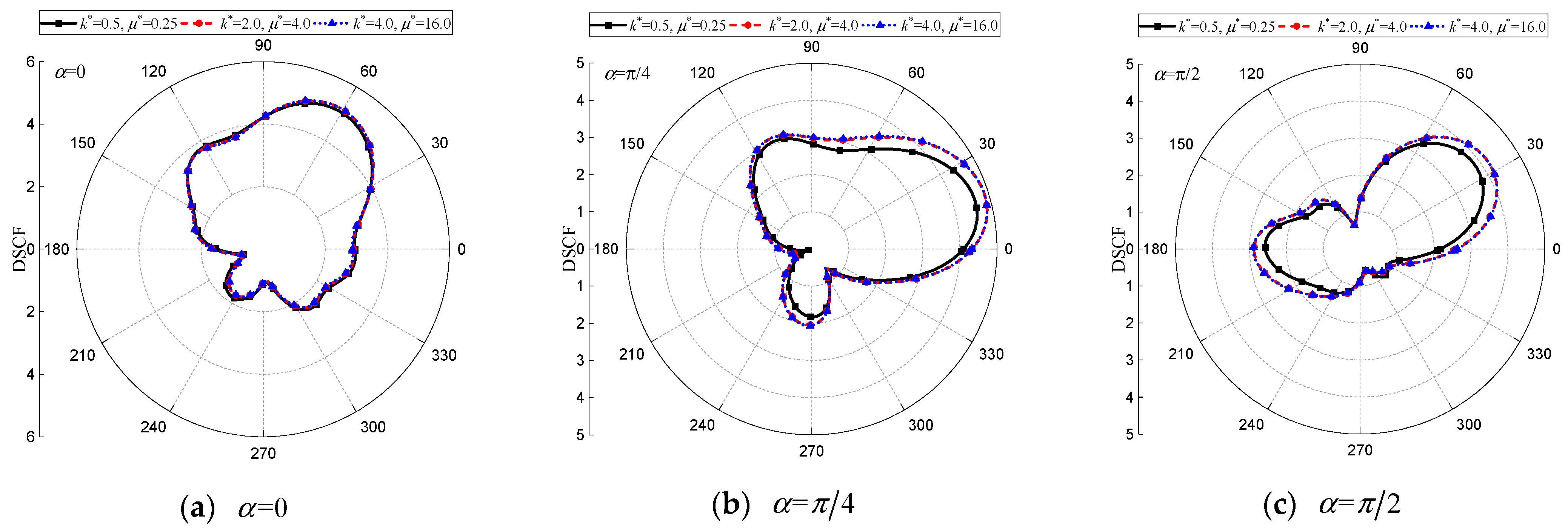
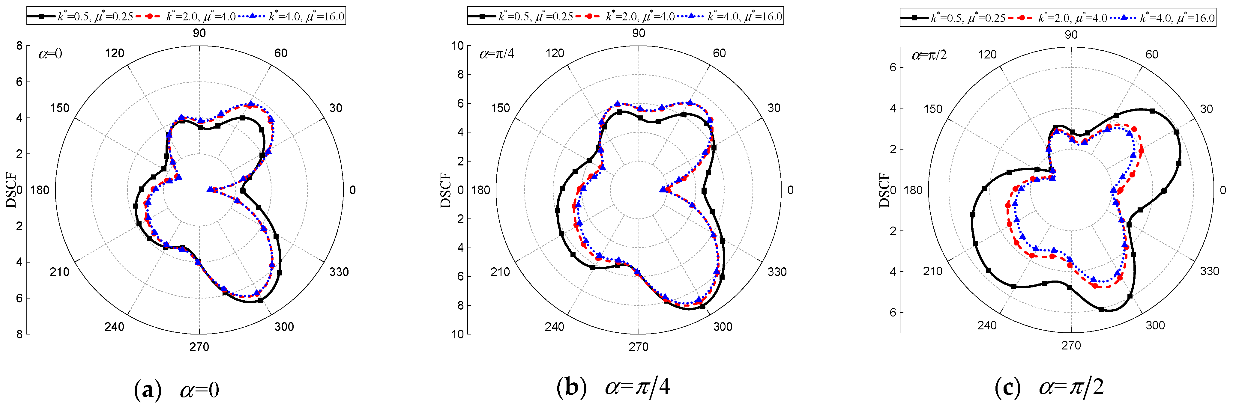
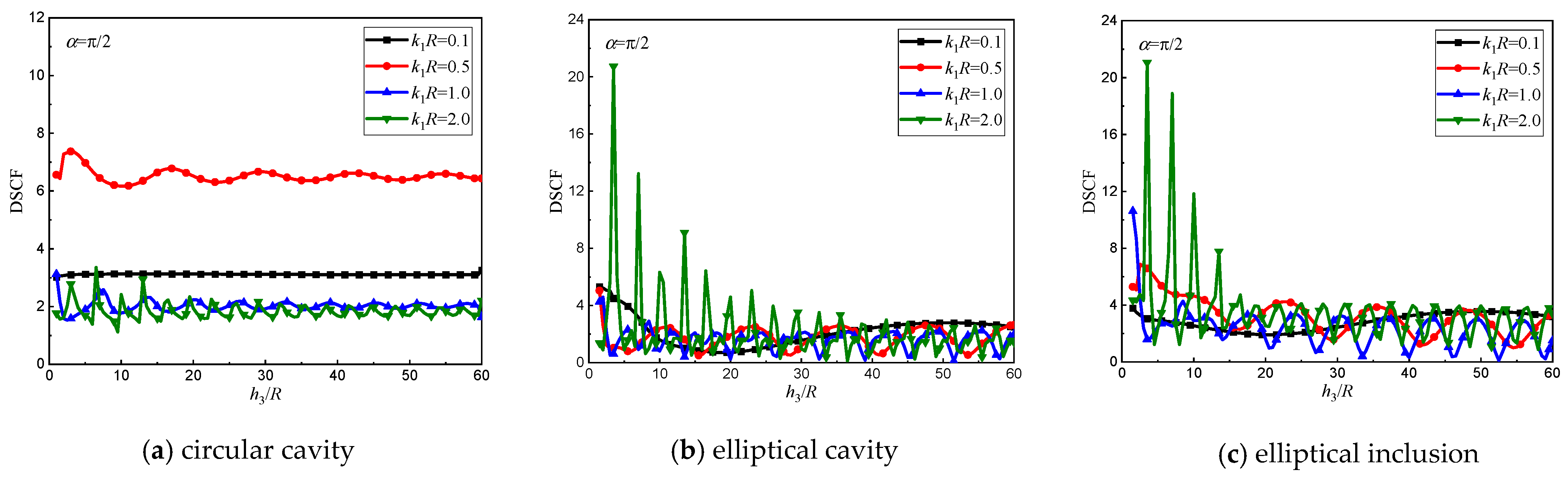
- With the rise in frequency of incident waves, the scattering field surrounding the cavities becomes more noticeable. When SH waves propagate through anisotropic media at horizontal or diagonal angles, they display distinct propagation characteristics and unique instructions. Moreover, the scattering field produced by the interaction between the complex structure (two cavities and an inclusion) and the bi-material interface is highly complex, especially when the complex structure is shallowly buried. Thus, dynamic stress concentration around the complex structure will be more pronounced when the cavities are located near the interface. Additionally, the distance between the elliptical cavity and the elliptical inclusion , wave-number ratio and shear modulus ratio of isotropic medium to inclusion influence slightly on DSCFs around the circular cavity within anisotropic medium, but a lot on dynamic response of the elliptical cavity and inclusion while exhibiting distinct variations with changing incidence angles of SH waves. Besides, the research presented in this article also demonstrates that wave-number ratio and shear modulus ratio between two halfspaces also significantly affect dynamic stress concentration around the cavities and inclusion, which should be focused on consideration in engineering design involving interface problems.
- The research conducted in this project has yielded valuable mechanical principles that can serve as a valuable reference for engineering practice. These principles have wide-ranging applications in fields such as mining engineering, seismic engineering, earth exploration, oil and gas exploration and development of underground structures, environmental engineering exploration, and quantitative non-destructive testing. The theoretical guidance provided in the presented paper is essential for investigating engineering problems involving formations with inclusions, holes, or cracks. By expanding the scope of this project’s research, we can further explore models of anisotropic bimaterials and multilayer media that incorporate irregular holes and inclusions as well as multiple defects incident by SHwave, Pwave, or SVwave. This endeavor is expected to generate additional significant research literature with immense practical value.
Author Contributions
Funding
Data Availability Statement
Conflicts of Interest
References
- Liu, D.K.; Gai, B.Z.; Tao, G.Y. Applications of the method of complex variables to dynamic stress concentrations. Wave Motion 1982, 4, 293–304. [Google Scholar] [CrossRef]
- Liu, D.K.; Lin, H. Scattering of SH-waves by circular cavities near biomaterial interface. Acta Mech. Solida Sin. 2003, 24, 197–204. [Google Scholar]
- Chen, T.Y.; Wang, H. Dynamic analysis of upright incident of SH-waves at semi-cylindrical interface with a circular lining structure. J. Tianjin Univ. 2006, 39, 1305–1309. [Google Scholar]
- Wang, G.Q.; Liu, D.K. Scattering of SH-wave by multiple circular cavities in half space. Earthq. Eng. Eng. Vib. 2002, 1, 36–44. [Google Scholar] [CrossRef]
- Xu, P.; Tie, Y.; Xia, T.D. Scattering of plane SH Waves by two separated circular tunnel linings. Northwest Seism. J. 2008, 30, 145–149. [Google Scholar]
- Wang, Y.S.; Qiu, Z.Y.; Yu, G.L. Scattering of SH waves from a partially debonded rigid elliptic cylinder. Soil. Dyn. Earthq. Eng. 2001, 21, 139–149. [Google Scholar] [CrossRef]
- Qi, H.; Yang, J. Dynamic analysis for circular inclusions of arbitrary positions near interfacial crack impacted by SH-wave in half-space. Eur. J. Mech. A Solids 2012, 36, 18–24. [Google Scholar] [CrossRef]
- Lu, J.F.; Wang, Y.S.; Cai, L. Scattering of SH wave by a crack terminating at the interface of bi-material. Chin. J. Theor. Appl. Mech. 2003, 35, 432–436. [Google Scholar]
- Yang, J.; Qi, H. Analysis of dynamic stress intensity factors for interfacial crack near shallow circular inclusion in bi-material half-space to SH wave. Acta Mech. 2016, 227, 3703–3714. [Google Scholar] [CrossRef]
- Bian, J.L.; Yang, Z.L.; Jiang, G.X.X.; Yang, Y.; Sun, M. Analytical solution to the SH wave scattering problem caused by a circular cavity in a half space with inhomogeneous modulus. Meccanica 2021, 56, 705–709. [Google Scholar] [CrossRef]
- Li, M.H.; Yang, Z.L.; Bian, J.L.; Yang, Y. Theoretical modeling and dynamic analysis of designable grillages for repairing material surface defect. Mech. Adv. Mater. Struct. 2024, 31, 12504–12511. [Google Scholar] [CrossRef]
- Yang, J.; Liu, S.; Yang, B.; Liu, Y. Scattering of SH waves in a bi-material half space with a circular hole and periodic type III interfacial cracks. Mech. Adv. Mater. Struct. 2023, 30, 2863–2871. [Google Scholar] [CrossRef]
- An, N.; Song, T.S.; Hou, G. Dynamic interaction between complex defect and crack in functionally graded magnetic-electro-elastic bi-materials. Mech. Adv. Mater. Struct. 2022, 30, 2748–2764. [Google Scholar] [CrossRef]
- Sheikhhassani, R.; Dravinski, M. Dynamic stress concentration for multiple multilayered inclusions embedded in an elastic half-space subjected to SH-waves. Wave Motion 2016, 62, 20–40. [Google Scholar] [CrossRef]
- Bagheri, R.; Monfared, M.M. In-plane transient analysis of two dissimilar nonhomogeneous half-planes containing several interface cracks. Acta Mech. 2020, 231, 3779–3797. [Google Scholar] [CrossRef]
- Yang, Z.L.; Yan, P.L.; Liu, D.K. Scattering of SH-waves and ground motion by an elastic cylindrical inclusion and a crack in half space. Chin. J. Theor. Appl. Mech. 2009, 41, 229–235. [Google Scholar]
- Xu, H.N.; Yang, Z.L.; Wang, S.S. Dynamics Response of Complex Defects near Bimaterials Interface by Incident Out-plane Waves. Acta Mech. 2016, 227, 1251–1264. [Google Scholar] [CrossRef]
- Wang, C.Y.; Balogunc, O.; Achenbach, J.D. Application of the reciprocity theorem to scattering of surface waves by an inclined subsurface crack. Int. J. Solids Struct. 2020, 207, 82–88. [Google Scholar] [CrossRef]
- Sung, J.C.; Wong, D.C. Effect of an inclusion on the interaction of elastic waves with a crack. Eng. Fract. Mech. 1995, 51, 679–695. [Google Scholar] [CrossRef]
- Ghafarollahi, A.; Shodja, H.M. Scattering of SH-waves by an elliptic cavity/crack beneath the interface between functionally graded and homogeneous half-spaces via multipole expansion method. J. Sound Vib. 2018, 435, 372–389. [Google Scholar] [CrossRef]
- Dravinski, M.; Sheikhhassani, R. Scattering of a plane harmonic SH wave by a rough multilayered inclusion of arbitrary shape. Wave Motion 2013, 50, 836–851. [Google Scholar] [CrossRef]
- Sonia, P.; Petia, D.; George, D.M. Elastic wave fields in a half-plane with free-surface relief, tunnels and multiple buried inclusions. Acta Mech. 2014, 225, 1843–1865. [Google Scholar] [CrossRef]
- Yu, C.W.; Dravinski, M. Scattering of plane harmonic P, SV and Rayleigh waves by a completely embedded corrugated elastic inclusion. Wave Motion 2010, 47, 156–167. [Google Scholar] [CrossRef]
- Andrade, H.C.; Trevelyan, J.; Leonel, E.D. Direct evaluation of stress intensity factors and T-stress for biomaterial interface cracks using the extended isogeometric boundary element method. Theor. Appl. Fract. Mech. 2023, 127, 104091. [Google Scholar] [CrossRef]
- Wei, P.J.; Zhang, Z.M. Scattering of inhomogeneous wave by viscoelastic interface crack. Acta Mech. 2002, 158, 215–225. [Google Scholar] [CrossRef]
- Liu, D.K.; Han, F. Scattering of plane SH wave by noncircular cavity in anisotropic media. J. Appl. Mech. Trans. ASME 1993, 60, 769–772. [Google Scholar] [CrossRef]
- Liu, D.K. Dynamic stress concentration around a circular cavity by SH wave in an anisotropic media. Acta Mech. Sin. 1988, 20, 443–452. [Google Scholar]
- Chen, Z.G. Dynamic stress concentration around shallow cylindrical cavity by SH wave in anisotropically elastic half-space. Roc. Soi Mech. 2012, 33, 899–905. [Google Scholar] [CrossRef]
- Chen, Z.G. Scattering of an orthotropic semi-cylindrical alluvial valley by SH waves. Earthq. Eng. Eng. Vib. 2016, 1, 68–74. [Google Scholar]
- Xu, H.N.; Zhang, J.W.; Yang, Z.L.; Lan, G.G.; Huang, Q.Y. Dynamic response of circular cavity and crack in anisotropic elastic half-space by out-plane waves. Mech. Res. Commun. 2018, 91, 100–106. [Google Scholar] [CrossRef]
- Lan, G.G.; Jiang, G.X.X.; Xu, H.N.; Qiu, F.Q.; Yang, Z.L. Analytical analysis of the interaction between cavities and a crack in bonded isotropic and anisotropic half spaces under SH wave. Mech. Adv. Mater. Struct. 2025, 32, 1518–1533. [Google Scholar] [CrossRef]
- Eslami, H.; Gatmiria, B. Two formulations for dynamic response of a cylindrical cavity in crossanisotropic porous media. Int. J. Numer. Anal. Meth. Geomech. 2010, 34, 331–356. [Google Scholar] [CrossRef]
- Sarkar, J.; Mandal, S.C.; Ghosh, M.L. Interaction of elastic waves with two coplanar griffith cracks in an orthotropic medium. Eng. Fract. Mech. 1994, 49, 411–423. [Google Scholar] [CrossRef]
- Shen, S.P.; Kuang, Z.B. Wave scattering from an interface crack in laminated anisotropic media. Mech. Res. Commun. 1998, 25, 509–517. [Google Scholar] [CrossRef]
- Zhou, Z.G.; Wu, L.Z.; Wang, B. The scattering of harmonic elastic anti-plane shear waves by two collinear cracks in anisotropic material plane by using the non-local theory. Meccanica 2006, 41, 591–598. [Google Scholar] [CrossRef]
- Boström, A.; Grahn, T.; Niklasson, A.J. Scattering of elastic waves by a rectangular crack in an anisotropic half-space. Wave Motion 2003, 38, 91–107. [Google Scholar] [CrossRef]
- Kumar, S.; Majhi, S.; Pal, P.C. Reflection and transmission of plane SH-waves in two semi-infinite anisotropic magnetoelastic media. Meccanica 2015, 50, 2431–2440. [Google Scholar] [CrossRef]
- Hasheminejad, S.M.; Maleki, M. Effect of Interface anisotropy on elastic wave propagation in particulate composites. J. Mech. 2013, 29, 7–26. [Google Scholar] [CrossRef]


Disclaimer/Publisher’s Note: The statements, opinions and data contained in all publications are solely those of the individual author(s) and contributor(s) and not of MDPI and/or the editor(s). MDPI and/or the editor(s) disclaim responsibility for any injury to people or property resulting from any ideas, methods, instructions or products referred to in the content. |
© 2025 by the authors. Licensee MDPI, Basel, Switzerland. This article is an open access article distributed under the terms and conditions of the Creative Commons Attribution (CC BY) license (https://creativecommons.org/licenses/by/4.0/).
Share and Cite
Xu, H.; Yang, C.; Wang, Y.; Lan, G.; Qiu, F. Dynamic Responseof Complex Defect near Anisotropic Bi-Material Interface by Incident Out-Plane Wave. Symmetry 2025, 17, 778. https://doi.org/10.3390/sym17050778
Xu H, Yang C, Wang Y, Lan G, Qiu F. Dynamic Responseof Complex Defect near Anisotropic Bi-Material Interface by Incident Out-Plane Wave. Symmetry. 2025; 17(5):778. https://doi.org/10.3390/sym17050778
Chicago/Turabian StyleXu, Huanan, Caizhu Yang, Yonghui Wang, Guoguan Lan, and Faqiang Qiu. 2025. "Dynamic Responseof Complex Defect near Anisotropic Bi-Material Interface by Incident Out-Plane Wave" Symmetry 17, no. 5: 778. https://doi.org/10.3390/sym17050778
APA StyleXu, H., Yang, C., Wang, Y., Lan, G., & Qiu, F. (2025). Dynamic Responseof Complex Defect near Anisotropic Bi-Material Interface by Incident Out-Plane Wave. Symmetry, 17(5), 778. https://doi.org/10.3390/sym17050778