Full-Element Analysis of Side-Channel Leakage Dataset on Symmetric Cryptographic Advanced Encryption Standard

Abstract

The application of deep learning in side-channel analysis faces critical challenges arising from dispersed public datasets—i.e., datasets collected from heterogeneous sources and platforms with varying formats, labeling schemes, and sampling settings—and insufficient sample distribution uniformity, characterized by imbalanced class distributions and long-tailed label samples. This paper presents a systematic analysis of symmetric cryptographic AES side-channel leakage datasets, examining how these issues impact the performance of deep learning-based side-channel analysis (DL-SCA) models. We analyze over 10 widely used datasets, including DPA Contest and ASCAD, and highlight key inconsistencies via visualization, statistical metrics, and model performance evaluations. For instance, the DPA_v4 dataset exhibits extreme label imbalance with a long-tailed distribution, while the ASCAD datasets demonstrate missing leakage features. Experiments conducted using CNN and Transformer models show that such imbalances lead to high accuracy for a few labels (e.g., label 14 in DPA_v4) but also extremely poor accuracy (<0.5%) for others, severely degrading generalization. We propose targeted improvements through enhanced data collection protocols, training strategies, and feature alignment techniques. Our findings emphasize that constructing balanced datasets covering the full key space is vital to achieving robust and generalizable DL-SCA performance. This work contributes both empirical insights and methodological guidance for standardizing the design of side-channel datasets.

1. Introduction

Side-channel attacks (SCAs) are cryptanalytic techniques that exploit the physical side effects of cryptographic operations, such as power consumption, electromagnetic radiation, etc., to extract sensitive information, such as cryptographic keys, from a system. Unlike traditional attacks, which target the algorithmic weaknesses of encryption schemes, an SCA focuses on the physical characteristics of the hardware used to make the cryptographic computations. These attacks can be highly effective because they do not rely on breaking the encryption itself but rather on exploiting the unintended leakage of information during the cryptographic operation. The relevance of side-channel analysis is especially significant in embedded systems and hardware implementations of cryptography, where physical characteristics are often accessible to an attacker. With the advent of deep learning techniques, SCAs have attracted a considerable amount of attention in recent years, as these methods can be used to process large volumes of data from side-channel measurements and identify hidden patterns that are otherwise difficult to detect.

Currently, several open-source datasets have been accumulated for the side-channel analysis community oriented towards symmetric encryption, asymmetric encryption, and hashing. This is due to domestic and foreign agents paying particular attention to the security field and the directions of security attacks and defense; as a result, long-term successive research gradually led to the formation of official public verification of these datasets. The previous experimental research and corresponding results have great open-source significance.

The evolution of SCA datasets can be roughly divided into three stages. First, in the early stage, DPA Contest [1], an official international competition, was accompanied by four versions of the dataset that came out of the tournament, with the trend of development ranging from the first generation, v1 [1], which is oriented towards DES analysis on ST 130 nm process ASICs, to the second generation, which is oriented towards the development of FPGA (AMD Xilinx and Intel Altera, America) development platforms via AES-128 analysis of v2 [2]; the third generation, v3 [3], in 2012 for FPGA (AMD Xilinx and Intel Altera, America) development and the implementation of AES; and finally the fourth generation, v4 [4,5], in 2014 for the analysis of AES soft implementations on smart cards; with the exception of v3, which is a cryptographic design, and its corresponding collection, several other versions of this dataset are available from the official website of the DPA Contest. The AES_RD [6,7] dataset, released in 2009, is an implementation of AES-128 on an 8-bit AVR microcontroller in which the cryptographic approach uses the floating average method to generate random delays. Although it is cryptographically protected, it is easy to crack the key using deep learning—specifically a CNN targeting spatial invariance. AES_HD [8,9] is a dataset that targets the power consumption and EM harvesting of an unprotected implementation of AES-128 on a SASEBO-G II FPGA (AMD Xilinx and Intel Altera, America) on-chip, but it has a high noise level, making it a more challenging target than, for example, DPA_v4.1. Despite this, it is not widely used because its cryptographic implementation is unprotected and uses the same key for encryption and decryption capture and analysis.

In the middle stage of development, the analysis objective included the implementation of protected cryptography, and the analysis method included the introduction of deep learning technology. The Northeastern University team continuously maintained the TeSCASE [10] dataset from 2014 to 2016, pioneering both masked and unmasked AES implementations on GPUs with power and timing harvesting; it also included ECC implementations, Keccak implementations, and EM-side information harvesting on ARM-based architectures. The team also made public a dataset called AES_HD_MM, which is a masked hardware AES implementation that has not been widely used in deep learning techniques, possibly because this dataset is older, and therefore many researchers are unaware of its availability. This dataset’s curve set and application have not been validated, and feedback has not yet been obtained; subsequent work will be carried out to detail its index structure and content, visually analyze it, and discuss it once results are obtained. From 2013 to 2017, the University of Cambridge team maintained the Grizzly [11] dataset, which is a record of power consumption for implementing unguarded AES-128 against the microcontroller 8-bit CPU Atmel XMEGA 256 A3U. In addition to this, the team has also made public the curves collected against Beta devices in Grizzly, the Panda Dataset for random template attacks using 16-bit test data, and side information leakage collection against SHA3-32bit and ASCON ciphers. In 2018, the international conference organization PANDA released the Panda2018 Challenge1 [12] dataset in a competition it organized; this dataset was also released for AES soft implementations. It is a collection of 1200 power consumption curves for standard AES-128 when encrypted in an AT89S52 cryptographic device. ASCAD [13,14,15] (ANSSI SCA Database) is a collection of side-channel analysis databases jointly developed by the French National Agency for the Security of Information Systems (ANSSI) and the CEA, designed to provide the SCA community with a database similar to the benchmarking reference of the MNIST database in machine learning. The entire dataset represents a de facto standard for evaluating deep learning-based SCAs. The version with random keys is not much more complex than the fixed-key version. Finally, these datasets also introduce novelty from a data management point of view, as they use the hdf5 dataset format. Recent studies have shown that for ASCAD_fixed_key, some bytes show first-order or univariate second-order leakage, which is unexpected for protected implementations. A new version of ASCADv2 has just recently been made publicly available, so there are not many results regarding its use. The information available for this version suggests that the dataset may be difficult to attack if it is assumed that the secret-sharing technique is not known, whereas it may be easy to attack if the sharing technique is known. The CHES_CTF_2018 [16] dataset proposed by Riscure Labs in the Netherlands (now acquired by Keysight) is harder to attack than ASCAD. 2020 CHES_CTF_2020 [17], on the other hand, is a measurement for mask implementations of Clyde-128 ciphers, with a total of seven sub-challenges, four of which are for software implementations and three of which are for hardware implementations.

In the third stage of work in this field, the migration of device targets was considered, while the targets of analysis were gradually shifted to other, more difficult types of cryptographic algorithms. Portability Dataset Portability (NDSS) [18] is designed for the EM side of information collection for the soft implementation of unguarded AES on Atmel Mega. It is therefore vulnerable to attacks, which makes it a less attractive target for deep learning. There are fewer datasets based on public key implementations, and Weissbart et al. [19,20] reported on a dataset pertaining to the targeting of unprotected Ed25519 (WolfSSL) on STM32, which makes it an unrealistic target. The Curve25519 μNaCl [21] dataset involved the targeting of a protected ECC soft implementation of STM32, making it a (somewhat) realistic target, but few results are available. The Curve25519 dataset [22] pertains to a protected implementation of EdDSA on STM32, with a different number of features and countermeasures. The above three datasets have been publicly available for a relatively short period, so only one paper [23] (written by this author’s team) has examined them.

This Section begins with a complete compilation and classification of the datasets according to their sources, target chip devices, cryptanalysis targets, types of analysis, and timeline of publication, as shown in

Table 1. Details of publicly available datasets (software-based).

	Targeted Chip Devices	Cryptographic	Type of Analysis	Name of Data Set	Traces (Features)	Time
1	SASEBO-W	AES-256 RSM	Electromagnetic	DPA contest_v4.1 [24]	100,000 (5000/4000)	2014
	ATMega-163	AES-128 RSM	Electromagnetic	DPA contest_v4.2 [25]	80,000 (1,704,400)	2015
2	8-bit Atmel AVR	Protected AES	Power consumption	AES_RD [6]	50,000 (3500)	2009
3	8-bit CPU Atmel XMEGA 256 A3U	AES-128	Power consumption	Grizzly [11]	-	2013 – 2017
				Grizzly: Panda	-
4	AT89S52	AES-128	Power consumption	Panda 2018 Challenge1 [12]	-	2018
5	STM32	AES-128	Electromagnetic	CHES_CTF2018 [16]	42,000 (650,000)	2018
6	ATMega	AES-128	Electromagnetic	ASCAD [13] (ASCADf, ASCADv1, ASCADv2)	60,000 (100,000)	2018
	ATMega	AES-128	Electromagnetic		300,000 (250,000)	2018
	STM32	AES-128	Electromagnetic		810,000 (1,000,000)	2021
7	Atmel Mega	AES-128	Electromagnetic	Portability [18]	50,000 (600)	2020
8	STM32	EdDSA	Electromagnetic	Ed25519 (WolfSSL) [20]	6400 (1000)	2019
	STM32	EdDSA	Electromagnetic	Curve25519 (μNaCL) [21]	5997 (5500)	2020
	STM32	EdDSA	Electromagnetic	Curve25519 [22]	300 (8000)	2020
	STM32	EdDSA	Electromagnetic	Curve25519 [22]	300 (1000)	2020

and

Table 2. Details on publicly available datasets (hardware-based).

	Targeted Chip Devices	Cryptographic	Type of Analysis	Name of Data Set	Traces (Features)	Time
1	SASEBO-GII	DES AES-128	Electromagnetic	DPA contest_v1 [1]	-	2008 – 2014
				DPA contest_v2 [1]	100,000 (3253)
				DPA contest_v3 [3]	-
2	SASEBO-GII	AES-128	Power consumption Electromagnetic	AES_HD [8]	50,000 (1250)	2018
3	SASEBO-GII	AES-128 MAC-Keccak	Power consumption Electromagnetic	TeSCASE [10] (AES_HD_MM)	5,600,000 (3500)	2014 – 2016
	Nvidia TeslaC2070 Nvidia Kepler K40	AES			-
	ARM Cortex M0+	ECC			-
4	Hardware	Clyde128		CHES_CTF_2020 [17]	+	2020

.

Despite their technical contributions, these datasets share several common limitations that hinder the generalization of DL-SCA methods. First, sample distribution imbalance is prevalent; datasets like DPA_v4 and ASCAD exhibit long-tailed or sparse label distributions, causing deep models to overfit for majority classes while ignoring minority ones. Second, incomplete feature coverage can be observed in many datasets where only partial encryption rounds or specific key bytes are represented, restricting model robustness. Third, inconsistency in data formats and key space coverage—including varied uses of plaintext/ciphertext alignment, desynchronization, and masking—introduces non-trivial preprocessing barriers and hinders standardized evaluation.

Therefore, rather than serving as plug-and-play resources for deep learning applications, current public SCA datasets must be carefully handled, aligned, and augmented to make them truly useful. In this work, we aim to bridge this gap by conducting a comprehensive, full-element analysis across over ten mainstream datasets (e.g., DPA_v4, ASCAD, AES_RD, and AES_HD), quantifying their structural flaws and demonstrating how these flaws directly impact the performance and generalizability of DL-SCA models. This will lay the foundation for proposing actionable strategies for improving dataset design and training protocols in the SCA domain.

The aim of this study is to optimize the structure of symmetric cipher datasets to address these challenges, facilitating more effective and reliable evaluations of cryptographic security using deep learning techniques. In this study, we carried out relevant experimental research work, and the main contributions are summarized as follows:

• This is the first systematic analysis of public datasets in the side-channel domain integrating the results of the analysis, elaborating the sources and uses of curves in public datasets, and developing data analysis visualization scripts to make index queries and perform point trace visualization for typical datasets.
• We have conducted an innovative full-elemental analysis of side-channel analysis datasets. To promote the application of deep learning techniques in this field, we carried out an elemental analysis of full-volume sample datasets and statistically analyzed the distribution of the number of labels when performing [0,255] key guessing.
• We designed experiments regarding the impact of masked label samples on the training of deep learning methods, exploring the specific effects of the total number of sample features and the uniformity of label samples on the model, to provide operational suggestions and methodological references for the original collection of the dataset, the integration of the preprocessing, and the complementation of the data label features.

The subsequent sections of this article are structured as follows: Section 2 will review related work and introduce existing datasets for side-channel analysis; Section 3 provides the results of a visual analysis of the datasets to reveal the feature differences between different datasets; Section 4 describes the design and analysis of the experiments using the CNN and Transformer architectures; and Section 5 summarizes the main contributions of this research and proposes future research directions.

2. Related Work

In the breakdown of datasets listed in the previous subsection, the most frequently used and methodologically improved dataset in the field of deep learning is the ASCAD [14,15,26,27,28,29,30,31,32,33,34,35,36,37] dataset, which is also the starting point for the development of the DL-SCA technique. In other representative studies, researchers tended to choose DPA_contest_v4 [26,27,30,31,33,35,38], AES_RD [26,30,31,34,35,38], AES_HD [26,30,31,35], CHES_CTF_2018 [36], CHES_CTF_2020 [37], etc. Targeting different datasets, that is, targeting different devices and cryptographic scenarios, requires a researcher to have a good understanding of the collection elements and sources of the dataset, a facet that also affects whether the implemented technical approach is effective and efficient.

Regarding instances wherein noise, or the signal-to-noise ratio, becomes the characteristic element of concern, Picek et al. [38] and Zaid et al. [30] first focused on the signal-to-noise situation of the dataset, accounting for the range of SNRs or the highest value of a single point at the location of the targeted attack in the dataset used for the experiments. Hajra et al. [37] pinpointed the location of the highest SNR according to the location of the highest SNR for a Clyde-128 on an ARM Cortex-M0 microcontroller to achieve specific leaked byte bits.

Regarding instances wherein sensitive operational features become an element of interest, Paguada et al. [29] computationally obtained spiking features in the distribution range of correlation coefficients before and after applying an S-box and masking, in addition to giving characteristic timestamps of signal-to-noise-ratio-sensitive leaks;

Regarding instances wherein data addition processing, such as random jitter, becomes an element of concern, Hajra et al. [35] provided informative and valuable information regarding adding set jitter {200, 400} to ASCAD, which, in this paper, is speculated to be able to simulate longer-distance curve acquisition offsets.

Scholars from various research institutions may encounter unique or common problems when using these public datasets. A summary of the issues this article responds to is given below:

• The format of the dataset is not yet uniform—The side-channel analysis community does not have a publicly available and centralized data center in which to house the datasets, with the data existing in a more dispersed state as shown in Table 3. Although HDF5 is advocated by some scholars and research institutes, each team still uses different instruments and equipment, and the file format of the capture export depends on one’s familiarity with the instrument used, such as the TRC file of a Liko oscilloscope, and algorithm dependence, such as in the development of NPY files in Python (a common problem).

  Table 3. Comparison of dataset storage formats.

  	hdf5	npy	trc	trs	bin
  Source	UIUC	-	LeCroy	TRS_bai(trs)	-
  Format Description	Structured Container	Multidimensional Array	Two-Dimensional Binary	Heterogeneous Text gbk	Two-Dimensional Binary
  Index Structure	Grouped Index	Single-File Index	Single-File Index	-	-
  Development Support	Universal	Python-Friendly	Matlab-Friendly	-	Universal
  Development Dependencies	h5py	numpy	LECROY_2_3 readTrc	-	-
  Storage Scale	TB-Level	Suitable for Lightweight Applications	TB-Level	TB-Level	TB-Level
  Main Advantages	Hierarchical | High-Scale Cross-Platform Application	Fast Reading and Writing			Lightweight and Universal
  Main Disadvantages	Complex API	Poor Portability Small Data Scale	Strong Instrument Dependence	High Space Utilization	-

  Table 3. Comparison of dataset storage formats.

  	hdf5	npy	trc	trs	bin
  Source	UIUC	-	LeCroy	TRS_bai(trs)	-
  Format Description	Structured Container	Multidimensional Array	Two-Dimensional Binary	Heterogeneous Text gbk	Two-Dimensional Binary
  Index Structure	Grouped Index	Single-File Index	Single-File Index	-	-
  Development Support	Universal	Python-Friendly	Matlab-Friendly	-	Universal
  Development Dependencies	h5py	numpy	LECROY_2_3 readTrc	-	-
  Storage Scale	TB-Level	Suitable for Lightweight Applications	TB-Level	TB-Level	TB-Level
  Main Advantages	Hierarchical | High-Scale Cross-Platform Application	Fast Reading and Writing			Lightweight and Universal
  Main Disadvantages	Complex API	Poor Portability Small Data Scale	Strong Instrument Dependence	High Space Utilization	-

• There is a lack of work on datasets for native encryption and decryption scenarios—Most of the teams in the SCA community and their research target deep learning attacks in non-native scenarios involving the grouping of ciphered AESs, with a preponderance of soft implementation analyses based on the type of MCU but very little hard implementation analyses (a common problem).
• Technology-related work concerns the implementation of deep learning for the sake of researching deep learning—The bottleneck in the development of DL-SCA technology around datasets is that it is not performed in the context of carrying out an actual attack but rather in the context of researching neural networks in search of a fixed paradigm. It is difficult to generalize results to real analysis scenarios (common problems) if the research in question relies exclusively on public datasets.
• Datasets without full samples—Most of the datasets in this domain are characterized by long-tailed data, with too few samples. In adjacent domains, Doan et al. [39] used historical time series to analyze the price volatility of cryptocurrencies, which is conceptually parallel to the volatility and non-uniformity of the characteristic distribution of labeled curves. This idea can help establish a methodology for addressing the non-uniformity and instability of the characteristic distribution of side-channel curves. Algorithmic execution can be lazy in the application of DL-SCA techniques, an issue analogous to the ‘misleading evaluation results due to model overfitting’ in the application of large models. When performing 8-bit or multi-bit key guessing in a divide-and-conquer fashion, algorithms automatically perform guessing wherever there are more samples. Insufficient samples for a single feature will lead to model-training bias, resulting in the key problem of overfitting (a common problem).
• Insufficient technical interpretations—In the case of ASCAD, for example, the raw curves are processed, 700 points are extracted to characterize the executable causes of sensitive operational partially executed analyses, and key byte guesses are often not made explicit (personality issues).
• Limiting factor in model performance—Despite the technical attempts made in relation to TransNet, EstraNet, and improved TransNet, small-feature-sample datasets only require lightweight models to achieve a single key byte, which then constrains the application of new-and-improved Transformer-based technical methods (the problem of individuality).

3. Materials and Methods

In this stage, we collected and integrated the public datasets that were collected and organized and integrated the development work of some visual analyses to clarify the datasets in a first-of-its-kind way reveal the most critical issues that emerge from deep learning methods and the statistical analyses of the features.

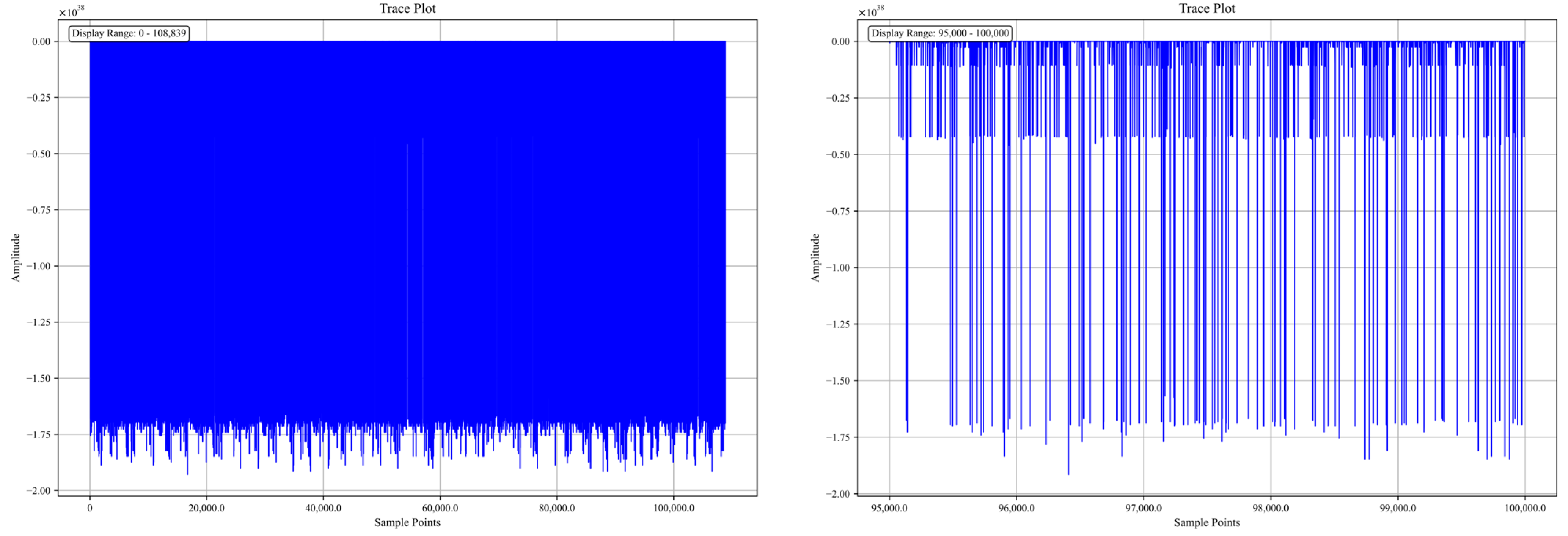
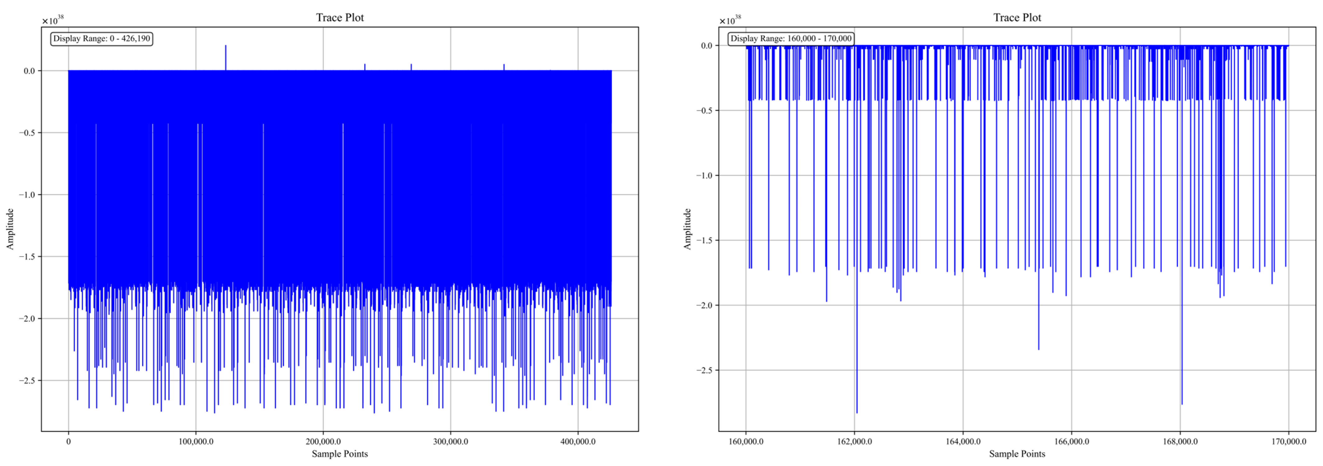
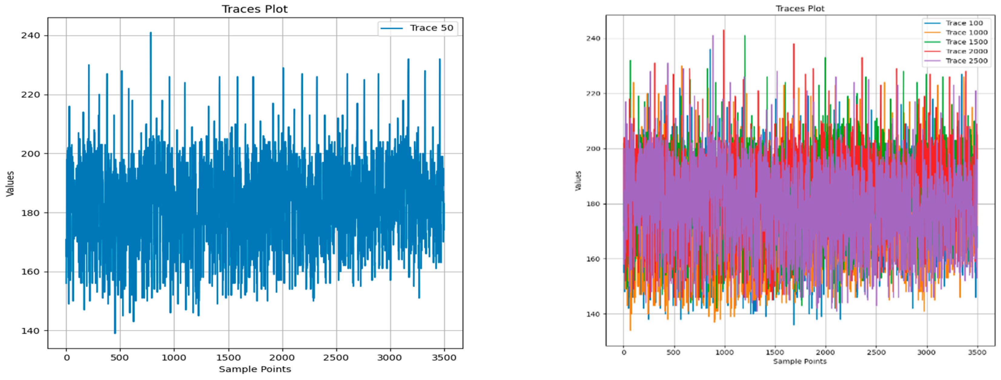
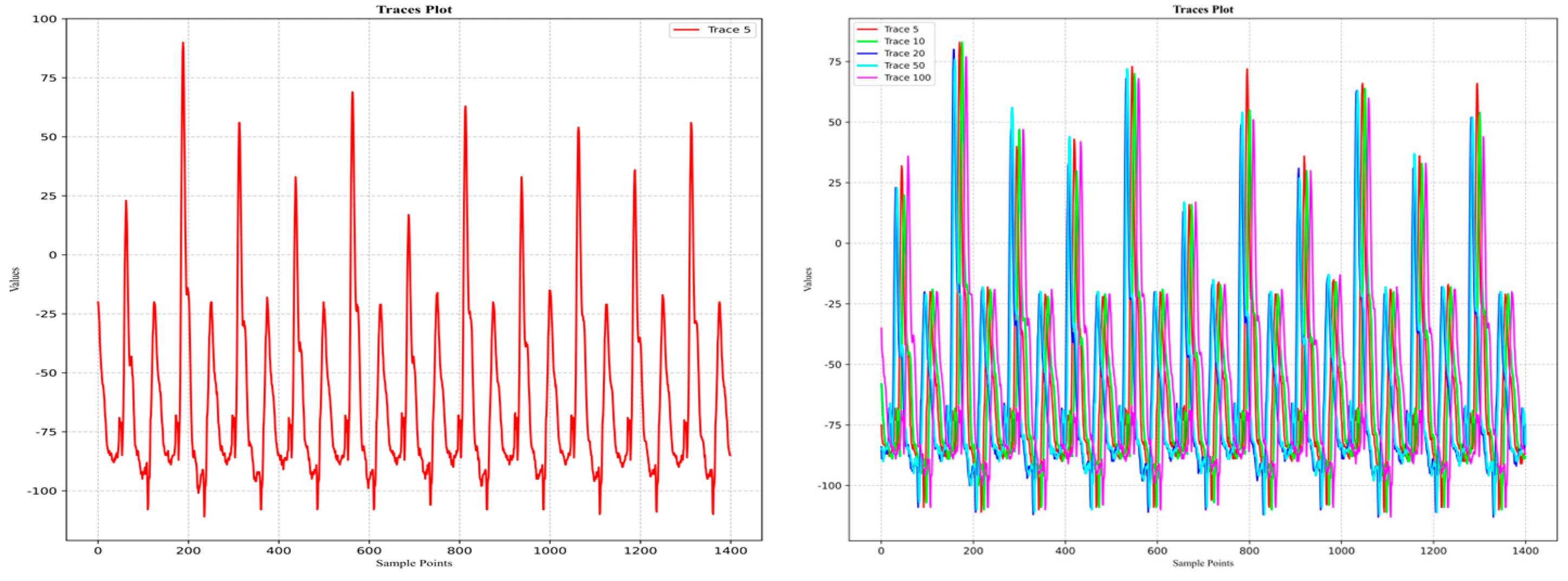
3.1. Visual Analysis of Dataset Traces

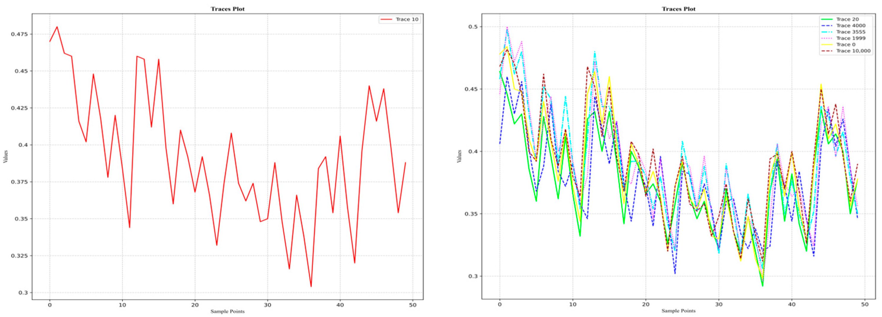
3.1.1. DPA Contest

DPA_v4.1 [24] targets multiple protected implementations of AES and implements the mask operation of AES-256 RSM on an Atmel ATMega-163 smartcard, which represents a standard target for simpler machine learning methods; however, it is not often used with deep learning methods as it is a very easy dataset to crack. Furthermore, the authors of the dataset report problems regarding the implemented countermeasures and first-order leakage of the power consumption curves. The contents of the DPA_v4.1 dataset index can be represented as follows:

$$\mathrm{DPA}\_\mathrm{v}4.1 \left\{\begin{array}{l} 00: \mathrm{shape} (\mathrm{10,000}, \mathrm{108,839})\\ 01: \mathrm{shape} (\mathrm{10,000}, \mathrm{108,839})\\ 02: \mathrm{shape} (\mathrm{10,000}, \mathrm{108,839})\\ \dots \dots \\ 09: \mathrm{shape} (\mathrm{10,000}, \mathrm{108,839})\end{array}\right.$$

(1)

It contains only 100,000 EM side information curves obtained via AES-256 (RSM) encryption of 10,000 random plaintexts using 1 key each. Since it is the original acquisition curve TRC file, each curve has 108,839 points. Visualizing one of the curves allows simple observation of the target characteristics, as shown in Figure 1.

In the 2015 v4.2 [25] version, with an improved masked implementation of AES-128 on the Atmel ATMega-163 smartcard (the curve includes full encryption), the DPA_v4.2 dataset index structure can be represented as follows:

$$\mathrm{DPA}\_\mathrm{v}4.2 \left\{\begin{array}{l} \mathrm{k}00: \mathrm{shape} (5000, \mathrm{426,190})\\ \mathrm{k}01: \mathrm{shape} (5000, \mathrm{426,190})\\ \mathrm{k}02: \mathrm{shape} (5000, \mathrm{426,190})\\ \dots \dots \\ \mathrm{k}15: \mathrm{shape} (5000, \mathrm{426,190})\end{array}\right.$$

(2)

It contains 5000 EM side information curves obtained via AES-128 encryption of 5000 random plaintexts using 16 keys each. These data are also given in the form of TRC files, and each curve has 426,190 points; again, visualizing one of the curves allows simple observation of the target features, as shown in Figure 2.

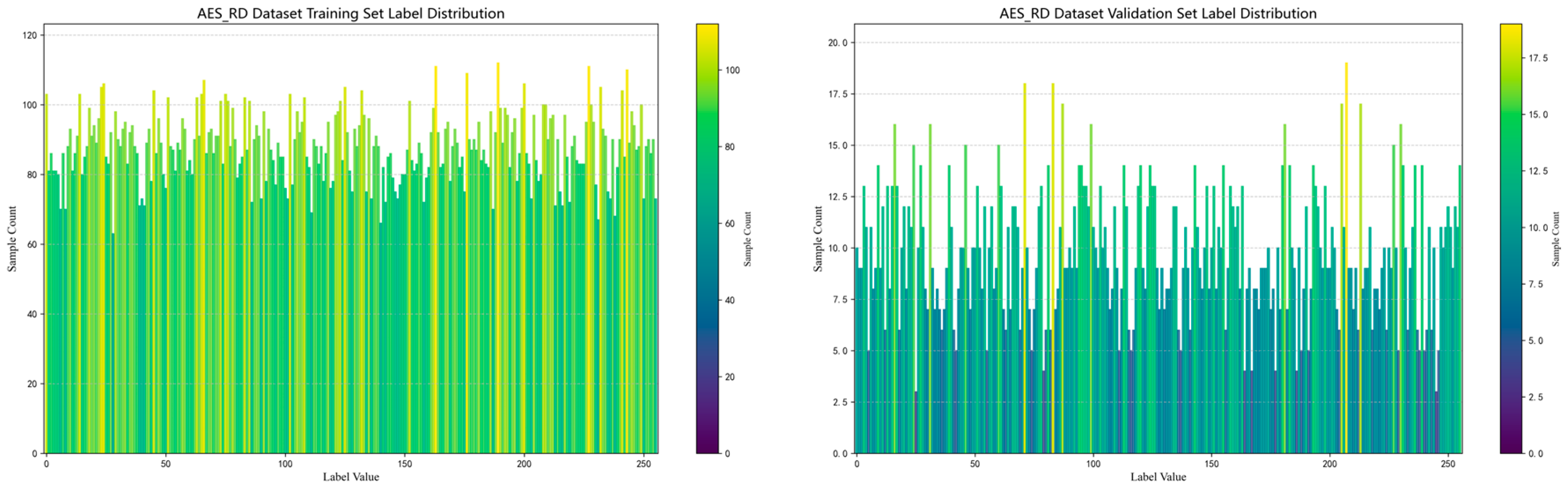
3.1.2. AES_RD

The AES_RD [6] dataset acquired in this study is not a collection of raw data, and its index content can be represented as follows:

$$\mathrm{AES}\_\mathrm{RD} \left\{\begin{array}{l} \mathrm{attack} \left\{\begin{array}{c} \mathrm{attack}\_\mathrm{labels}: \mathrm{shape} (\mathrm{25,000}, )\\ \mathrm{attack}\_\mathrm{plaintext}: \mathrm{shape} (\mathrm{25,000}, 16)\\ \mathrm{attack}\_\mathrm{traces}: \mathrm{shape} (\mathrm{25,000}, 3500)\end{array}\right.\\ \mathrm{profiling}\left\{\begin{array}{c} \mathrm{profiling}\_\mathrm{labels}: \mathrm{shape} (\mathrm{25,000}, )\\ \mathrm{profiling}\_\mathrm{plaintext}: \mathrm{shape} (\mathrm{25,000}, 16)\\ \mathrm{profiling}\_\mathrm{traces}: \mathrm{shape} (\mathrm{25,000}, 3500)\end{array}\right.\\ \mathrm{key}: \mathrm{shape}(16, )\\ \mathrm{mask}: \mathrm{None}\end{array}\right.$$

(3)

It contains an attack, the profiling of two curve collections, and the analysis target key. In terms of data characteristics, the collection of curves contains one-to-one correspondence of attack (25,000)/profiling (25,000) labels, plaintexts, and curve power consumption physical quantity information. An example curve Trace 50 in attack_trace was opened and visualized, as shown in Figure 3, which characterizes the EM-side information of 3500 points corresponding to the 50th set of 128-bit plaintexts in an operation encrypted using a fixed key, as recorded by the collection. The five example curves in profiling_trace were opened and visualized, as shown in Figure 3, as an overlay.

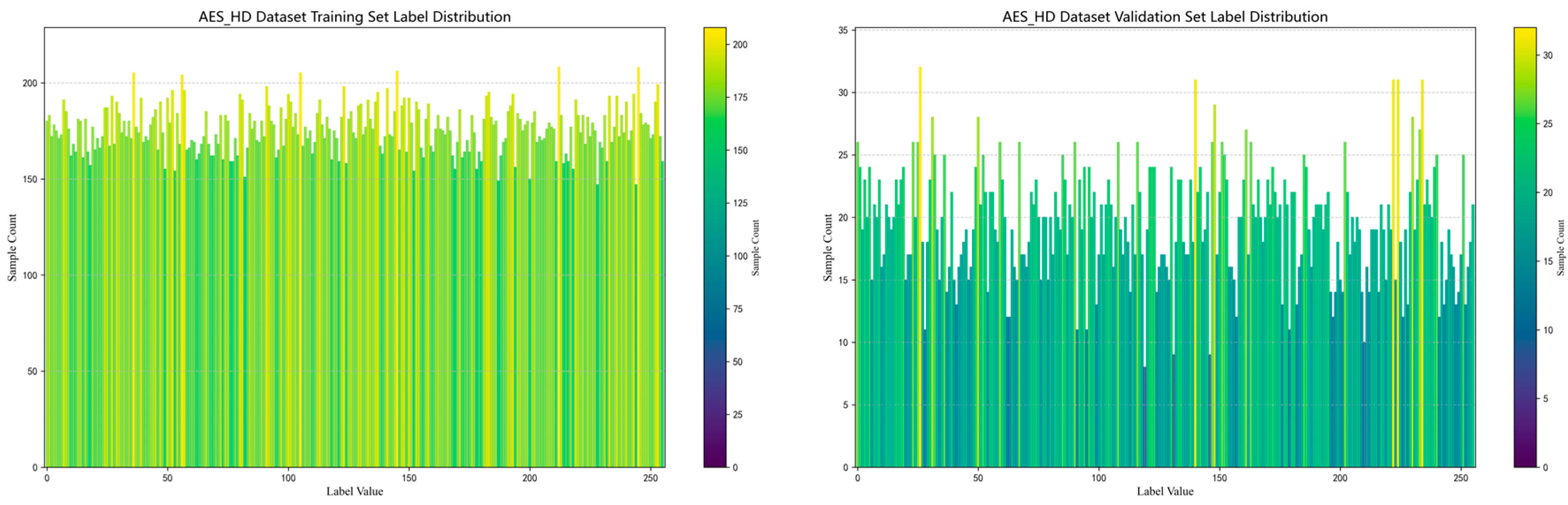
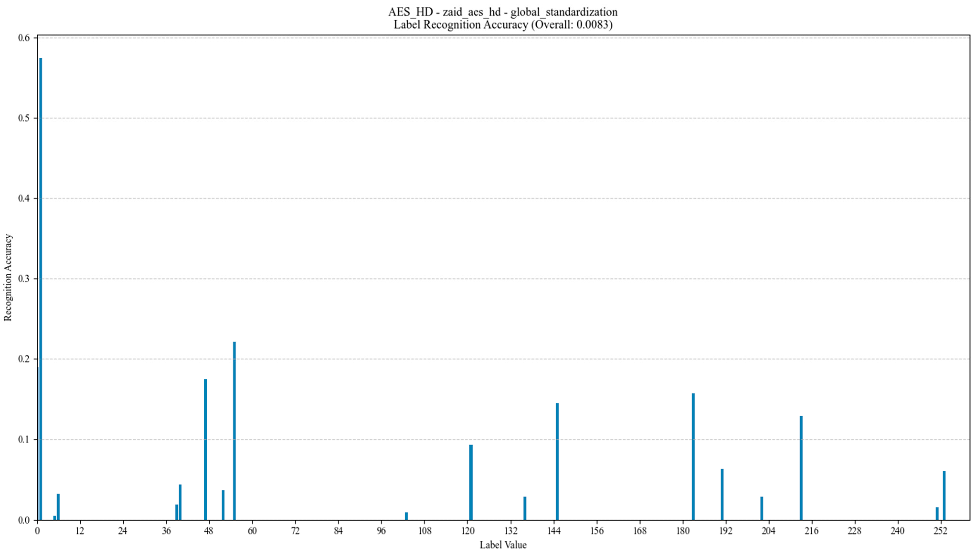
3.1.3. AES_HD

The AES_HD [8] dataset acquired in this study is in HDF5 format with a more rational storage and indexing structure, denoted as

$$\mathrm{AES}\_\mathrm{HD} \left\{\begin{array}{l} \mathrm{Attack}\_\mathrm{traces} \left\{\begin{array}{l}\mathrm{metadata}\left\{\begin{array}{l}\mathrm{ciphertext}: \mathrm{shape} (5000, 16)\\ \mathrm{plaintext}: \mathrm{shape} (5000, 16)\\ \mathrm{key}: (5000, 16)\end{array}\right.\\ \mathrm{traces}: \mathrm{shape} (5000, 1250)\end{array}\right.\\ \mathrm{Profiling}\_\mathrm{traces}\left\{\begin{array}{l}\mathrm{metadata}\left\{\begin{array}{l}\mathrm{ciphertext}: \mathrm{shape} (\mathrm{45,000}, 16)\\ \mathrm{plaintext}: \mathrm{shape} (\mathrm{45,000}, 16)\\ \mathrm{key}: (\mathrm{45,000}, 16)\end{array}\right.\\ \mathrm{traces}: \mathrm{shape} (\mathrm{45,000}, 1250)\end{array}\right.\end{array}\right.$$

(4)

It contains two groups, Attack_traces and Profiling_traces. In terms of data characteristics, the two groups contain 5000 and 25,000 curves of power consumption and electromagnetic physical quantity information and corresponding plaintext, respectively. An example curve Trace 100 in the Attack_traces group was opened and visualized, as shown in Figure 4 (left), which characterizes the EM-side information of the 100th set of 128-bit plaintexts recorded at 1250 points in the operation encrypted via a fixed key. The four example curves in profiling_trace were opened and visualized on top of each other, as shown in Figure 4 (right).

3.1.4. Grizzly

The Grizzly [11] dataset acquired in this study is in raw curve RAW format, and the storage and indexing structure is characterized by and has the advantage of containing multiple curves within the RAW curve file, which can be represented as

$$\mathrm{Grizzly}\left\{\begin{array}{l}\mathrm{Device}1: \mathrm{Alpha}\_\mathrm{shape}(\mathrm{448,266}, \mathrm{986,185,764})\\ \mathrm{Device}2: \mathrm{Beta}\_\mathrm{shape}(\mathrm{448,266}, \mathrm{986,185,764})\\ \mathrm{Device}3: \mathrm{Beta} \mathrm{Bis}\_\mathrm{shape}(\mathrm{448,266}, \mathrm{986,185,764})\\ \mathrm{Device}4: \mathrm{Gamma}\_\mathrm{shape}(\mathrm{448,266}, \mathrm{986,185,764})\\ \mathrm{Device}5: \mathrm{Delta}\_\mathrm{shape}(\mathrm{448,266}, \mathrm{986,185,764})\end{array}\right.$$

(5)

It contains five raw acquisition files from five devices, each containing 448,266 curves. Opening Trace_30 on an Alpha device and visualizing it (as shown in Figure 5 (left)) allowed us to characterize the 30th set of 986,185,764 power consumption traces recorded through the raw acquisition of the 128-bit plaintext in an operation encrypted using a random key. We opened multiple curves on an Alpha device and visualized them in an overlaid fashion, as shown in Figure 5 (right).

3.1.5. Panda2018 Challenge

The Panda2018 Challenge1 dataset acquired in this study is in raw curve BIN format, with the BIN storage and indexing structure of a single file characterizing only a single curve, denoted as

$$\mathrm{Panda} 2018 \mathrm{Challenge}1: \left\{\mathrm{shape}(1044, \mathrm{61,049})\right.$$

(6)

It contains only 1044 single curve files, with each curve containing 61,049 power consumption point traces, characterizing the power leakage of the 128-bit plaintext ciphertext operation process. One of the curves was opened and visualized, as shown in Figure 6.

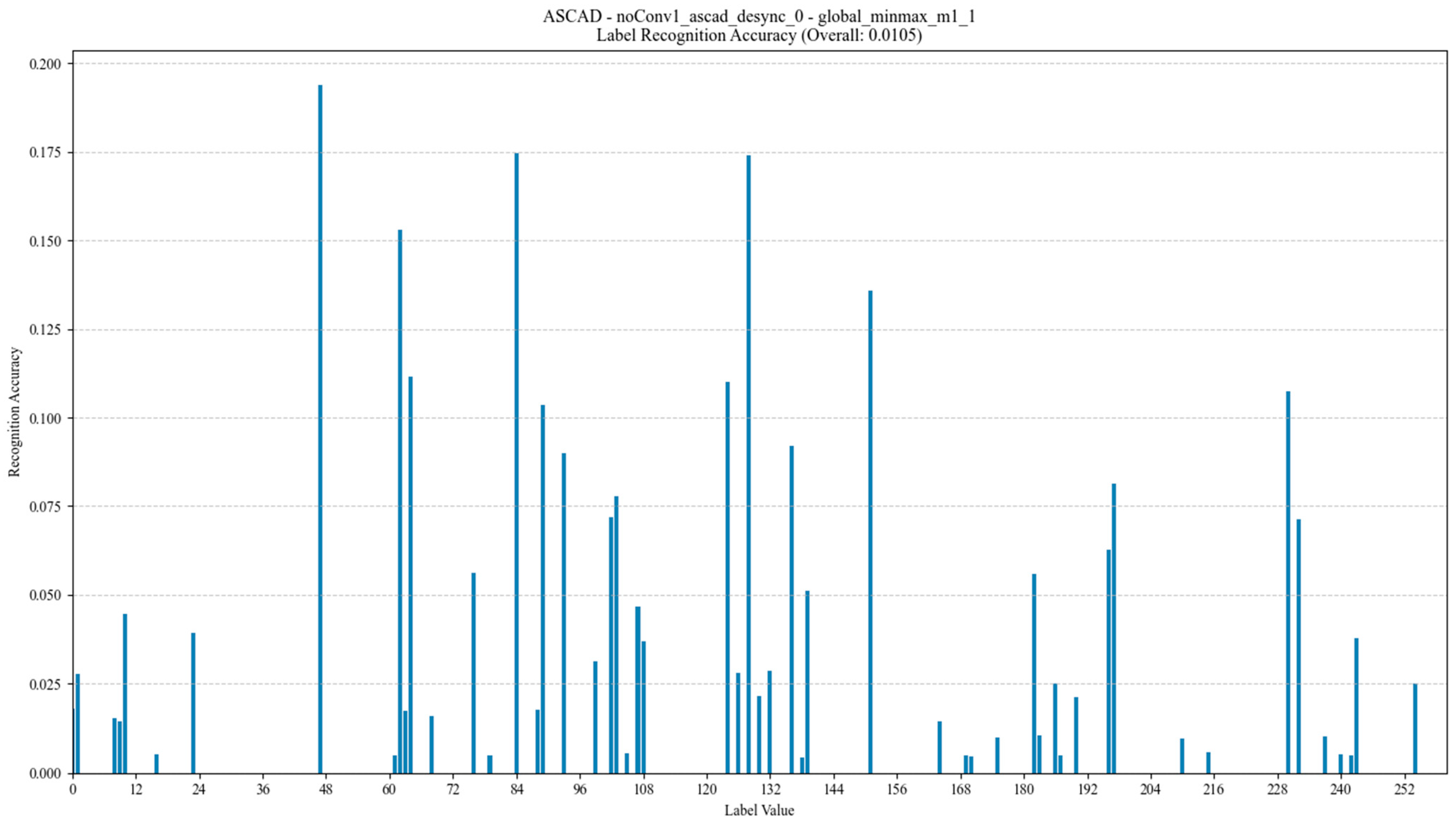
3.1.6. ASCAD

Details of the three versions of the ASCAD dataset [13,14,15] are given below:

• For the soft implementation of AES-128 on ATMega with fixed key EM-side information leakage ASCAD_fixed_key, the storage and index structure can be represented as

$$\mathrm{fixed}\_\mathrm{key}\left\{\begin{array}{l}\mathrm{ASCAD}.\mathrm{h}5\left\{\begin{array}{l}\mathrm{Attack}\_\mathrm{traces} \left\{\begin{array}{l}\mathrm{label}:\mathrm{shape} (\mathrm{10,000}, 1)\\ \mathrm{metadata}\left\{\begin{array}{l}\mathrm{ciphertext}: \mathrm{shape} (\mathrm{10,000}, 16)\\ \mathrm{plaintext}: \mathrm{shape} (\mathrm{10,000}, 16)\\ \mathrm{key}: (\mathrm{10,000}, 16)\\ \mathrm{masks}:\mathrm{shape} (\mathrm{10,000}, 16)\\ \mathrm{desync}:\mathrm{shape} (\mathrm{10,000}, 16)\end{array}\right.\\ \mathrm{traces}: \mathrm{shape} (\mathrm{10,000}, 700)\end{array}\right.\\ \mathrm{Profiling}\_\mathrm{traces}\left\{\begin{array}{l}\mathrm{label}:\mathrm{shape} (\mathrm{50,000}, 1)\\ \mathrm{metadata}\left\{\begin{array}{l}\mathrm{ciphertext}: \mathrm{shape} (\mathrm{50,000}, 16)\\ \mathrm{plaintext}: \mathrm{shape} (\mathrm{50,000}, 16)\\ \mathrm{key}: (\mathrm{50,000}, 16)\\ \mathrm{masks}:\mathrm{shape} (\mathrm{10,000}, 16)\\ \mathrm{desync}:\mathrm{shape} (\mathrm{10,000}, 16)\end{array}\right.\\ \mathrm{traces}: \mathrm{shape} (\mathrm{50,000}, 700)\end{array}\right.\end{array}\right.\\ \mathrm{ASCAD}\_\mathrm{desync}50.\mathrm{h}5 (\mathrm{as} \mathrm{above})\\ \mathrm{ASCAD}\_\mathrm{desync}100.\mathrm{h}5 (\mathrm{as} \mathrm{above})\\ \mathrm{ATMega}8515\_\mathrm{raw}\_\mathrm{traces}.\mathrm{h}5:\mathrm{traces}: \mathrm{shape} (\mathrm{60,000}, \mathrm{100,000})\end{array}\right.$$

(7)

There are two main groups, Attack_traces and Profiling_traces, which contain 10,000 and 50,000 curves of EM physical quantities with corresponding plaintext, key, mask, and desynchronization values in terms of data characteristics. An example curve regarding Trace 10 in the Attack_traces group was opened and visualized, as shown in Figure 7 (left), characterizing the EM-side information of 700 points recorded via the acquisition of the first key byte of the S-box operation corresponding to the 128-bit plaintext of group 10 in the operation encrypted using a fixed key. The five example curves in profiling_trace were opened and visualized in a superimposed fashion, as shown in Figure 7 (right), where desync50/100 represents the curves adopting random numbers before [0,50] and [0,100] for jitter processing at the timestamps.

2.

For the soft implementation of AES-128 on ATMega with random key EM-side information leakage ASCAD_vriable_key, the storage and index structure is represented as

$$\mathrm{variable}\_\mathrm{key}\left\{\begin{array}{l}\mathrm{vriable}.\mathrm{h}5\left\{\begin{array}{l}\mathrm{Attack}\_\mathrm{traces} \left\{\begin{array}{l}\mathrm{label}:\mathrm{shape} (\mathrm{100,000}, 1)\\ \mathrm{metadata}\left\{\begin{array}{l}\mathrm{plaintext}: \mathrm{shape} (\mathrm{100,000}, 16)\\ \mathrm{key}: (\mathrm{100,000}, 16)\\ \mathrm{masks}:\mathrm{shape} (\mathrm{100,000}, 16)\\ \mathrm{desync}:\mathrm{shape} (\mathrm{100,000}, 16)\end{array}\right.\\ \mathrm{traces}: \mathrm{shape} (\mathrm{100,000}, 1400)\end{array}\right.\\ \mathrm{Profiling}\_\mathrm{traces}\left\{\begin{array}{l}\mathrm{label}:\mathrm{shape} (\mathrm{200,000}, 1)\\ \mathrm{metadata}\left\{\begin{array}{l}\mathrm{plaintext}: \mathrm{shape} (\mathrm{200,000}, 16)\\ \mathrm{key}: (\mathrm{200,000}, 16)\\ \mathrm{masks}:\mathrm{shape} (\mathrm{200,000}, 16)\\ \mathrm{desync}:\mathrm{shape} (\mathrm{200,000}, 16)\end{array}\right.\\ \mathrm{traces}: \mathrm{shape} (\mathrm{200,000}, 1400)\end{array}\right.\end{array}\right.\\ \mathrm{vriable}\text{-}\mathrm{desync}50.\mathrm{h}5\left(\mathrm{as} \mathrm{above}\right)\\ \mathrm{vriable}\text{-}\mathrm{desync}100.\mathrm{h}5\left(\mathrm{as} \mathrm{above}\right)\\ \mathrm{atmega}8515\text{-}\mathrm{raw}\text{-}\mathrm{traces}.\mathrm{h}5:\mathrm{traces}: \mathrm{shape} (\mathrm{300,000}, \mathrm{250,000})\end{array}\right.$$

(8)

There are two main groups, Attack_traces and Profiling_traces, which contain 100,000 and 200,000 curves of EM physical quantities with corresponding plaintext, key, mask, and desynchronization values in terms of data characteristics. An example curve Trace 5 in the Attack_traces group was opened and visualized, as shown in Figure 8 (left), which characterizes the EM-side information of 1400 points recorded through the acquisition of the first key byte after the S-box operation corresponding to the 128-bit plaintext of group 5 encrypted using a fixed key. The five example curves in profiling_trace were opened and visualized in a superimposed manner, as shown in Figure 8 (right), where desync50/100 represents the curves adopting random numbers before [0,50] and [0,100] for jitter processing at the timestamp.

3.

For the AES-128 soft implementation of the no-secret sharing ASCAD_v2 on STM32, the storage and index structure is represented as follows:

$$\mathrm{v}2\left\{\begin{array}{l}\mathrm{v}2\text{-}\mathrm{extraced}.\mathrm{h}5\left\{\begin{array}{l}\mathrm{Attack}\_\mathrm{traces} \left\{\begin{array}{l}\mathrm{label}\left\{\begin{array}{l}\mathrm{alpha}\_\mathrm{mask}:\mathrm{shape} (\mathrm{10,000}, 1)\\ \mathrm{beta}\_\mathrm{mask}:\mathrm{shape} (\mathrm{10,000}, 1)\\ \mathrm{sbox}\_\mathrm{masked}:\mathrm{shape} (\mathrm{10,000}, 16)\\ \mathrm{sbox}\_\mathrm{masked}\_\mathrm{with}\_\mathrm{perm}:\mathrm{shape} (\mathrm{10,000}, 16)\\ \mathrm{perm}\_\mathrm{index}:\mathrm{shape} (\mathrm{10,000}, 16)\end{array}\right.\\ \mathrm{metadata}\left\{\begin{array}{l}\mathrm{plaintext}: \mathrm{shape} (\mathrm{100,000}, 16)\\ \mathrm{key}: (\mathrm{100,000}, 16)\\ \mathrm{masks}:\mathrm{shape} (\mathrm{100,000}, 16)\\ \mathrm{desync}:\mathrm{shape} (\mathrm{100,000}, 16)\end{array}\right.\\ \mathrm{traces}: \mathrm{shape} (\mathrm{100,000}, 1400)\end{array}\right.\\ \mathrm{Profiling}\_\mathrm{traces}\left\{\begin{array}{l}\mathrm{label}\left\{\begin{array}{l}\mathrm{alpha}\_\mathrm{mask}:\mathrm{shape} (\mathrm{10,000}, 1)\\ \mathrm{beta}\_\mathrm{mask}:\mathrm{shape} (\mathrm{10,000}, 1)\\ \mathrm{sbox}\_\mathrm{masked}:\mathrm{shape} (\mathrm{10,000}, 16)\\ \mathrm{sbox}\_\mathrm{masked}\_\mathrm{with}\_\mathrm{perm}:\mathrm{shape} (\mathrm{10,000}, 16)\\ \mathrm{perm}\_\mathrm{index}:\mathrm{shape} (\mathrm{10,000}, 16)\end{array}\right.\\ \mathrm{metadata}\left\{\begin{array}{l}\mathrm{plaintext}: \mathrm{shape} (\mathrm{200,000}, 16)\\ \mathrm{key}: (\mathrm{200,000}, 16)\\ \mathrm{masks}:\mathrm{shape} (\mathrm{200,000}, 16)\\ \mathrm{desync}:\mathrm{shape} (\mathrm{200,000}, 16)\end{array}\right.\\ \mathrm{traces}: \mathrm{shape} (\mathrm{200,000}, 1400)\end{array}\right.\end{array}\right.\\ \mathrm{v}2\text{-}\mathrm{stm}32\text{-}\mathrm{conso}\text{-}\mathrm{raw}\text{-}\mathrm{traces}1/2/3/4.\mathrm{h}5\left(\mathrm{Same} \mathrm{as} 5\right)\\ \mathrm{v}2\text{-}\mathrm{stm}32\text{-}\mathrm{conso}\text{-}\mathrm{raw}\text{-}\mathrm{traces}5.\mathrm{h}5\left\{\begin{array}{l}\mathrm{info}:\mathrm{shape}(0, 0)\\ \mathrm{metadata}\left\{\begin{array}{l}\mathrm{plaintext}: \mathrm{shape} (\mathrm{200,000}, 16)\\ \mathrm{key}: (\mathrm{200,000}, 16)\\ \mathrm{masks}:\mathrm{shape} (\mathrm{200,000}, 16)\\ \mathrm{desync}:\mathrm{shape} (\mathrm{200,000}, 16)\end{array}\right.\\ \mathrm{traces}:\mathrm{shape} (\mathrm{100,000}, \mathrm{1,000,000})\end{array}\right.\\ \mathrm{v}2\text{-}\mathrm{stm}32\text{-}\mathrm{conso}\text{-}\mathrm{raw}\text{-}\mathrm{traces}6/7/8.\mathrm{h}5\left(\mathrm{Same} \mathrm{as} 5\right)\end{array}\right.$$

(9)

It contains two main groups, Attack_traces and Profiling_traces, which contain 100,000 and 200,000 curves of EM physical quantity information and corresponding plaintext, key, mask, and desynchronization values in terms of data characteristics. The difference is that this version also contains four masks and one index parameter label. An example curve, Trace 10 in the Attack_traces group, was opened and visualized, as shown in Figure 9 (left), which characterizes the EM side of the 15,000 points of information corresponding to the first key byte after the S-box operation for the 10th set of 128-bit plaintexts encrypted with a fixed key, as captured and recorded. The four example curves in profiling_trace were opened and visualized in a superimposed state, as shown in Figure 9 (right).

3.1.7. CHES_CTF_2018/2020

CHES_CTF_2018 [16] is less used due to the lack of support for the public version, which has only 10,000 curves per analyzed set, and its storage and index structure are represented as

$$\mathrm{CHES}\_\mathrm{CTF}\_2018\left\{\begin{array}{l}\mathrm{attacking}\_\mathrm{data}: \mathrm{shape} (5000, 48)\\ \mathrm{attacking}\_\mathrm{traces}: \mathrm{shape} (5000, 2200)\\ \mathrm{profiling}\_\mathrm{data}: \mathrm{shape} (\mathrm{45,000}, 48)\\ \mathrm{profiling}\_\mathrm{traces}: \mathrm{shape} (\mathrm{45,000}, 2200)\end{array}\right.,$$

(10)

containing four data indexes, attacking_data, attacking_traces, profiling_data, and profiling_traces. We opened one curve, Trace 5, of the set of attack curves and visualized it, as shown in Figure 10 (left). It characterizes the AES-128 encryption corresponding to the 10th set of data computation and produces an EM-side information leak. We opened the five example curves in profiling_trace and visualized them in a superimposed fashion, as shown in Figure 10 (right).

3.1.8. Portability (NDSS)

The portability dataset [18] is currently the only publicly available dataset that can be used to study the impact of AES portability, and its storage and indexing structure is represented below:

$$\mathrm{Portability}\left(\mathrm{NDSS}\right)\left\{\begin{array}{l}\mathrm{c}1\mathrm{k}1\left\{\begin{array}{l}\mathrm{ctext}\_\mathrm{val}\_5000\mathrm{tr}: \mathrm{shape} (5000, 16)\\ \mathrm{ptext}\_\mathrm{val}\_5000\mathrm{tr}: \mathrm{shape} (5000, 16)\\ \mathrm{traces}\_\mathrm{val}\_5000\mathrm{tr}\_50\mathrm{pt}: \mathrm{shape} (5000, 50)\\ \mathrm{traces}\_\mathrm{val}\_5000\mathrm{tr}\_600\mathrm{pt}: \mathrm{shape} (5000, 600)\\ \mathrm{ctext}\_\mathrm{pro}\_\mathrm{40,000}\mathrm{tr}: \mathrm{shape} (\mathrm{40,000}, 16)\\ \mathrm{ptext}\_\mathrm{pro}\_\mathrm{40,000}\mathrm{tr}: \mathrm{shape} (\mathrm{40,000}, 16)\\ \mathrm{traces}\_\mathrm{pro}\_\mathrm{40,000}\mathrm{tr}\_50\mathrm{pt}: \mathrm{shape} (\mathrm{40,000}, 50)\\ \mathrm{traces}\_\mathrm{pro}\_\mathrm{40,000}\mathrm{tr}\_600\mathrm{pt}: \mathrm{shape} (\mathrm{40,000}, 600)\end{array}\right.\\ \mathrm{c}2\mathrm{k}1, \mathrm{c}2\mathrm{k}2, \mathrm{c}3\mathrm{k}1, \mathrm{c}4\mathrm{k}1, \mathrm{c}4\mathrm{k}1\mathrm{A}, \mathrm{c}4\mathrm{k}3\left(\mathrm{as} \mathrm{above}\right)\end{array}\right.$$

(11)

It contains 56 sets of curves, which are modeled (pro) and analytically verified (val) sets of the data corresponding to the 4 types of keys and 4 types of plain ciphertexts. One, Trace 10 of the [c1k1] 50 pt and 600 pt groupings, was opened and visualized, as shown in Figure 11 (left) and Figure 11 (right), respectively, characterizing the EM-side information leakage resulting from the AES-128 encryption computation corresponding to data in group 10, and five example curves in the profiling_trace were opened and visualized in superimposed form, as shown in Figure 12 (left) and Figure 12 (right).

Through visualization and qualitative comparative analysis of the eight datasets, we found the following:

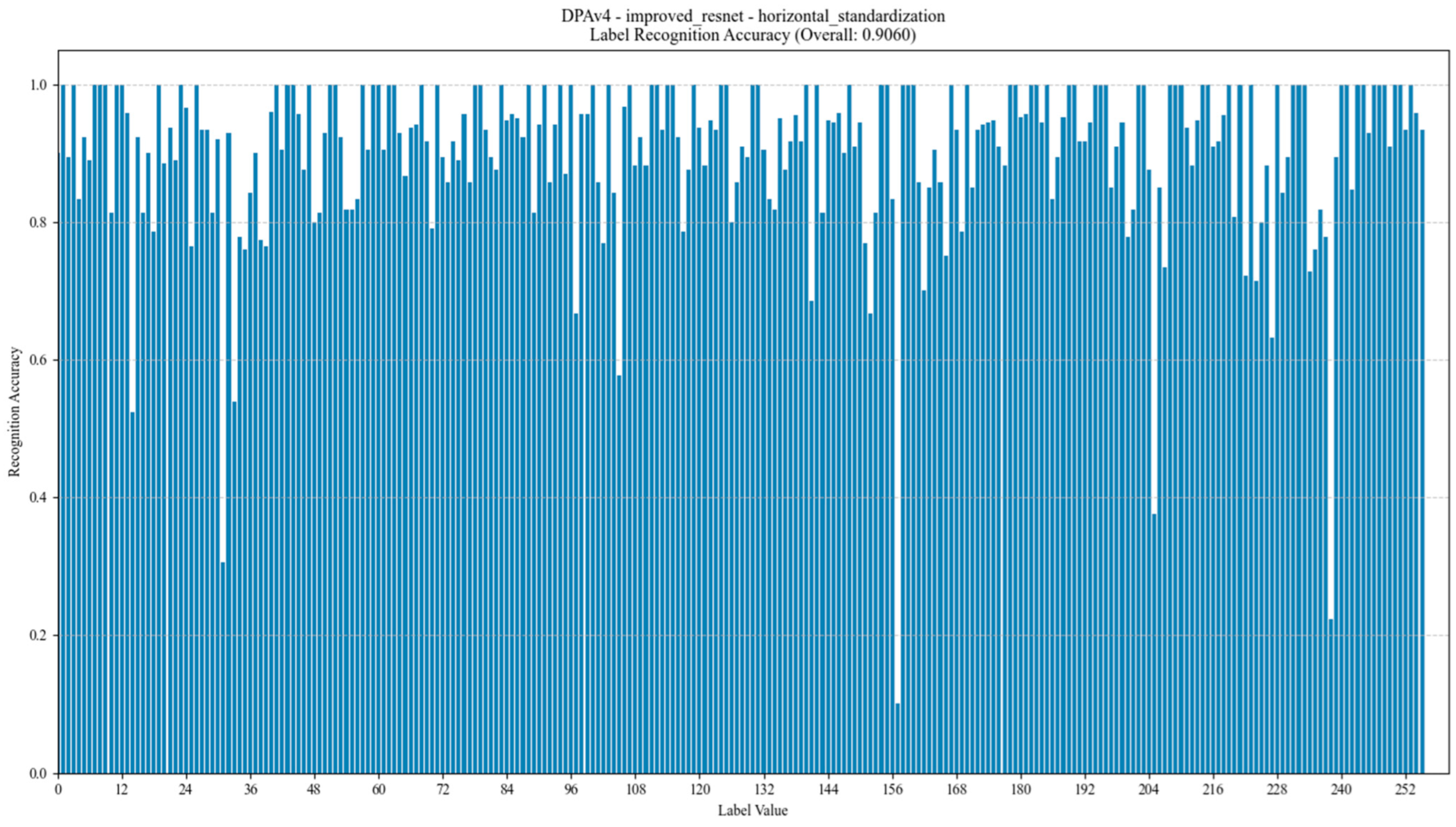
• An uneven distribution of labels is the main problem affecting model training performance, especially in the DPA_v4 and ASCAD datasets, where the distribution of labels shows a long-tail effect. For example, in the DPA_v4 dataset, the number of samples for label 14 is 10,000, while the number of labels other labels is only about 1000, leading to poor model training with a small number of labels. The ASCAD dataset also suffers from the problem of uneven labeling, and even though it has a large number of samples (up to 50,000), there is still a problem consisting of a small number of samples for some labels, leading to a significant degradation in the performance of the deep learning model, especially when making predictions on samples with few labels with low accuracy.
• Noise level has a significant impact on model training. The AES_RD and AES_HD datasets are noisy, which makes deep learning model training more challenging. Taking the AES_RD dataset as an example, even though it contains 25,000 samples, the training of the model is significantly affected by the high percentage of noise, especially for labels with higher accuracy (e.g., Label 14), where the model accuracy stays high, but for noisy labels, the accuracy is low.
• A balance between sample size and feature dimensionality is crucial for model training. Although the sample sizes of the Grizzly and Panda2018 datasets are relatively small (448,266 and 1044 samples, respectively), they provide high-quality feature data, making them more suitable for training low-complexity models. In contrast, the AES_HD and ASCAD datasets provide a large number of samples (e.g., 50,000 samples for AES_HD) and are suitable for training deep learning models, but they still suffer from label imbalance and feature inconsistency.
• Standardization of datasets will yield better results, especially for the AES_RD, AES_HD, and ASCAD datasets, and their curve processing is the most standardized and better suited for the application of deep learning techniques.

3.2. Overfitting Analysis of CNNs and Transformers

By combining the modeling and non-modeling classifications from side-channel analysis and the basic composition of the aforementioned dataset, it can be uniformly represented as

$$\left\{\begin{array}{l}{\mathrm{D}}_{\mathrm{p}\mathrm{r}\mathrm{o}\mathrm{f}\mathrm{i}\mathrm{l}\mathrm{i}\mathrm{n}\mathrm{g}}={\left\{\overrightarrow{{\mathrm{l}}_{\mathrm{i}}},{\mathrm{p}}_{\mathrm{i}},{\mathrm{k}}_{\mathrm{i}}\right\}}_{\mathrm{i}=1,\dots ,{\mathrm{N}}_{\mathrm{p}}}={\left\{{\overrightarrow{\mathrm{l}}}_{\mathrm{i}},{\mathrm{z}}_{\mathrm{i}}\right\}}_{\mathrm{i}=1,\dots ,{\mathrm{N}}_{\mathrm{p}}}\\ {\mathrm{D}}_{\mathrm{t}\mathrm{r}\mathrm{a}\mathrm{i}\mathrm{n}}={\left\{\overrightarrow{{\mathrm{l}}_{\mathrm{i}}},{\mathrm{p}}_{\mathrm{i}},{\mathrm{k}}_{\mathrm{i}}\right\}}_{\mathrm{i}=1,\dots ,{\mathrm{N}}_{\mathrm{p}}}\\ {\mathrm{D}}_{\mathrm{t}\mathrm{e}\mathrm{s}\mathrm{t}}={\left\{\overrightarrow{{\mathrm{l}}_{\mathrm{i}}},{\mathrm{p}}_{\mathrm{i}},{\mathrm{k}}_{\mathrm{i}}\right\}}_{\mathrm{i}=1,\dots ,{\mathrm{N}}_{\mathrm{p}}}\\ {\mathrm{D}}_{\mathrm{a}\mathrm{t}\mathrm{t}\mathrm{a}\mathrm{c}\mathrm{k}}={\left\{\overrightarrow{{\mathrm{l}}_{\mathrm{i}}},{\mathrm{p}}_{\mathrm{i}}\right\}}_{\mathrm{i}=1,\dots ,{\mathrm{N}}_{\mathrm{a}}}\end{array}\right.$$

(12)

where ${\mathrm{l}}_{\mathrm{i}}$, ${\mathrm{p}}_{\mathrm{i}}$, and ${\mathrm{k}}_{\mathrm{i}}$ represent the leakage curve, plaintext, and key information, respectively, which are the key elements for analyzing the curve dataset. Here, ${\mathrm{p}}_{\mathrm{i}}$ can also be replaced with ${\mathrm{c}}_{\mathrm{i}}$ for performing decryption-guessing analysis.

To continue the previous work on some backbone network technology, we must continue to improve a certain benchmark method to achieve better evaluation metrics on the benchmark dataset, thus solidifying the formation of the SOTA method. In this study, CNN and Transformer backbone networks were selected: firstly, the general expression of the model was established:

$${\overrightarrow{\mathrm{g}}}_{\mathrm{CNN}}:\overrightarrow{\mathrm{l}}\mapsto \widehat{\mathrm{g}}(\overrightarrow{\mathrm{l}})=\mathrm{s}\circ {\left[\lambda \right]}^{{\mathrm{n}}_1}\circ {[\xi \circ {[\alpha \circ \gamma ({\overrightarrow{\mathrm{l}}}_{\mathrm{n}}\left)\right]}^{{\mathrm{n}}_2}]}^{{\mathrm{n}}_3}=\overrightarrow{\mathrm{y}}$$

(13)

where $\mathrm{s}$ represents the output layer; $\lambda$ represents the fully connected layer; $\alpha$ represents the activation function; $\xi$ introduces the pooling layer parameters; $\gamma$ introduces the convolutional layer parameters; and $\circ$ indicates the nesting and connection forms of the model components. According to our understanding of the Transformer structure, an analogy for the CNN’s general expression can be expressed as

$${\overrightarrow{\mathrm{g}}}_{\mathrm{Transformer}}: \overrightarrow{\mathrm{l}}\mapsto \widehat{\mathrm{g}}\left(\overrightarrow{\mathrm{l}}\right)=\mathrm{s}\circ {\phi }^{{\mathrm{n}}_4}\circ [\alpha \circ {\mu }_{\mathrm{Q},\mathrm{K},\mathrm{V}}^{{\mathrm{n}}_3}\circ {\rho }^{{\mathrm{n}}_2}\circ \epsilon ({\overrightarrow{\mathrm{l}}}_{\mathrm{n}}\left)\right]=\overrightarrow{\mathrm{y}}$$

(14)

where $\mathrm{s}$ represents the classification/regression head, i.e., the output layer; $\phi$ represents the feed-forward network; $\alpha$ represents the activation function; ${\mu }_{\mathrm{Q},\mathrm{K},\mathrm{V}}$ represents the attention mechanism, e.g., adopting the multi-head self-attention mechanism, flash-attention, etc.; ${\rho }^{{\mathrm{n}}_2}$ represents the position-coding layer; $\epsilon$ represents the input embedding layer; and $\circ$ indicates the nesting and connection forms of the model components.

Combined with the advantages of deep neural networks in solving classification problems [40,41], the tendency is to construct approximate models directly:

$${\overrightarrow{\mathrm{g}}}_{\mathrm{k}}:(\overrightarrow{\mathrm{l}}, \mathrm{p})\mapsto \mathrm{P}{[ \mathrm{P},\mathrm{K}=(\mathrm{p}, \mathrm{k}) | \overrightarrow{L}=\overrightarrow{\mathrm{l}} ]}_{\mathrm{k}\in \mathcal{K}}$$

(15)

We can apply the input of new plaintext $\mathrm{p}$ in the attack set ${\mathrm{D}}_{\mathrm{attack}}$ to observe the speculative classification of the new leakage $\overrightarrow{\mathrm{l}}$ candidate keys obtained from the collection. Then, the key discriminative classification can be performed by processing $\overrightarrow{\mathrm{y}}{=\mathrm{g}}_{\overrightarrow{L},\mathrm{P}}(\overrightarrow{\mathrm{l}}, \mathrm{p})$ and the key candidate key $\widehat{\mathrm{k}}={\mathrm{argmax}}_{\mathrm{k}}\overrightarrow{\mathrm{y}}\left[\mathrm{k}\right]$. The key discriminative classification of the curved plaintexts of the entire set of attacks on ${({\overrightarrow{\mathrm{l}}}_{\mathrm{i}},{\mathrm{p}}_{\mathrm{i}})}_{\mathrm{i}=1,\dots ,{\mathrm{N}}_{\mathrm{a}}}$ can be performed by using the strategy of greatest likelihood estimation to introduce the key-scoring vector ${\overrightarrow{\mathrm{d}}}_{{\mathrm{N}}_{\mathrm{a}}}\left[\mathrm{k}\right]$, which can be computed as follows:

$${\overrightarrow{\mathrm{d}}}_{{\mathrm{N}}_{\mathrm{a}}}\left[\mathrm{k}\right]={\displaystyle {\prod }_{\mathrm{i}=1}^{{\mathrm{N}}_{\mathrm{a}}}{\overrightarrow{\mathrm{y}}}_{\mathrm{i}}[\mathrm{k}]}$$

(16)

$${\overrightarrow{\mathrm{y}}}_{\mathrm{i}}[\mathrm{k}]={\mathrm{g}}_{\overrightarrow{L},\mathrm{P}}({\overrightarrow{\mathrm{l}}}_{\mathrm{i}},{\mathrm{p}}_{\mathrm{i}})[\mathrm{k}]$$

(17)

Then, the score vector can be expanded as follows:

$${\overrightarrow{\mathrm{d}}}_{{\mathrm{N}}_{\mathrm{a}}}\left[\mathrm{k}\right]={\displaystyle {\prod }_{\mathrm{i}=1}^{{\mathrm{N}}_{\mathrm{a}}}\mathrm{P}\left[\left(\mathrm{P},\mathrm{K}\right)=\left({\mathrm{p}}_{\mathrm{i}},\mathrm{k}\right)|\overrightarrow{\mathrm{L}}={\overrightarrow{\mathrm{l}}}_{\mathrm{i}}\right]}={\displaystyle {\prod }_{\mathrm{i}=1}^{{\mathrm{N}}_{\mathrm{a}}}\frac{\mathrm{P}\left[\overrightarrow{\mathrm{L}}={\overrightarrow{\mathrm{l}}}_{\mathrm{i}}|\left(\mathrm{P},\mathrm{K}\right)=\left({\mathrm{p}}_{\mathrm{i}},\mathrm{k}\right)\right]}{{\mathrm{f}}_{\overrightarrow{\mathrm{L}}}({\overrightarrow{\mathrm{l}}}_{\mathrm{i}})}}\times {\mathrm{f}}_{\left(\mathrm{P},\mathrm{K}\right)}({\mathrm{p}}_{\mathrm{i}},\mathrm{k}),$$

(18)

where ${\overrightarrow{\mathrm{y}}}_{\mathrm{i}}$ represents the output of the model, and the $\mathrm{k}$th coordinate of the score vector is the score corresponding to the key candidate key. The accumulation of model outputs yields the scores of key candidate keys and forms a vector of greatest likelihood estimates.

In training, a loss function calculation is introduced to evaluate the degree of inconsistency between the predicted and true values from model training. Cross-entropy loss (CE-LOSS) can be used for outputting the predicted labels ${\mathrm{y}}_{\mathrm{ij}}$ or the predicted probabilities ${\widehat{\mathrm{y}}}_{\mathrm{ij}}$ and the true labels or the true value deviations until convergence:

$${\mathrm{Loss}}_{\mathrm{CE}}=-{\displaystyle \frac{1}{\mathrm{N}}}{\displaystyle {\sum }_{\mathrm{i}=1}^{\mathrm{N}}{\displaystyle {\sum }_{\mathrm{j}=1}^{\mathrm{K}}{\mathrm{y}}_{\mathrm{ij}}\log ( {\widehat{\mathrm{y}}}_{\mathrm{ij}})}}$$

(19)

Since the guessing accuracy corresponds to the correctness of the key extracted candidates, researchers specializing in DL-SCA algorithms still adopt the guessing-accuracy metric. The model’s training and testing classification accuracy on the dataset itself can be calculated as follows:

$$\mathrm{Acc}.={\displaystyle \frac{\mathrm{TP}+\mathrm{TN}}{\mathrm{TP}+\mathrm{TN}+\mathrm{FP}+\mathrm{FN}}}$$

(20)

where TP stands for true case, TN stands for true-negative case, FP stands for false-positive case, and FN stands for false-negative case. Such a calculation expression is still relatively abstract, and the concrete application can be expressed using the following formula:

$$\mathrm{acc}({\overrightarrow{\mathrm{g}}}_{\mathrm{k}}{, \mathrm{D}}_{\mathrm{train}}{, \mathrm{D}}_{\mathrm{test}})={\displaystyle \frac{\left|\left\{{\overrightarrow{\mathrm{l}}}_{\mathrm{i}}{,\mathrm{p}}_{\mathrm{i}},\mathrm{k}*\in {\mathrm{D}}_{\mathrm{test}}| \hat{\mathrm{k}}={\mathrm{argmax}}_{\mathrm{k}}{ \mathrm{y} \to }_{\mathrm{i}}\left[\mathrm{k}\right]\right\}\right|}{\left|{\mathrm{D}}_{\mathrm{test}}\right|}}$$

(21)

Whether from the perspective of model structure parameter design, attention mechanism, feature engineering, or data enhancement, improvements can be achieved based on the above principles. This leads to innovations in effectiveness and enhancements in analysis efficiency. In deep learning technology, the practice of adjusting parameters in this way is often referred to as “alchemy”. Strong hypothesis experiments on side-channel analysis datasets aim to improve technical methods, even when the results are already known. The LOSS curve results of model training are often obtained before the target results are obtained. In order to carry out experimental research presented in this paper, the advanced algorithm model presented at the CHES conference in the side-channel field was selected for reproduction and improvement. As an example, the typical CNN variant and Transformer variant training LOSS curves for the AES_HD dataset are shown in Figure 13, Figure 14 and Figure 15. When there is a case where the validation set LOSS cannot be reduced, it indicates that when performing 8-bit or multi-bit key guessing in a divide-and-conquer manner, the algorithm automatically performs guessing wherever there is a large distribution of samples. In this case, the number of individual feature samples is insufficient, which will surely lead to model training bias and overfitting problems, and an effective expansion of the number of dataset curves or feature supplementation is required. In this regard, the comprehensive dataset proposed by Yadulla et al. [42] is a good reference.

We believe that increasing the number of samples in the dataset and the number of sample features up to the full number of samples, as opposed to imposing random jitter and data augmentation, are the key ways in which to promote the development of the new round of DL-SCA technology and push the technology towards representing real attack scenarios. For data preprocessing and feature alignment, the techniques of signal clustering and feature extraction applied by Wahyuningsih and Chen [43] using TF-IDF vectorization and K-means can also provide technical references.

3.3. Feature Statistical Analysis

In terms of deep learning interpretability, the focus is on labeled features, regardless of whether the topic is the convolutional operation of CNNs or the multi-head attention of the Transformer architecture. An insufficient number of samples or an uneven distribution of the dataset results in an insufficient number of features in the dataset. Insufficient feature dimensionality during training will result in a situation where models with fewer parameters will learn better. By analogy with the empirical analysis conducted by Wahyuningsih and Chen [44], the distribution of label features in the dataset has a significant impact on the classification accuracy of CNN and Transformer models. The full sample characteristics used for side-channel analysis can be defined as having sufficient power consumption curve characteristics corresponding to each of the 256 labels [0,255]. To quantitatively explore the data distribution of labels in typical datasets, the number of features of [0,255] labels in the DPA_v4, AES_RD, AES_HD, and ASCAD datasets were counted, as shown in Figure 16, Figure 17, Figure 18 and Figure 19.

It can be seen that the DPA_v4 dataset has few samples and the most inhomogeneous labeled data, and the remaining three datasets also show different degrees of long-tailed data. To explore the specific effects of the total number of sample features and the uniformity of labeled samples on the model, we designed further experiments to mask the effects of certain labeled samples on the training to provide operational suggestions and methodological references for the original collection of datasets and the integration of preprocessing data and to complement data-labeling features.

In training CNNs or transformers, dataset inconsistencies such as uneven sample distributions, missing features, and noisy data can significantly impact model performance. In particular, datasets like DPA_v4 and ASCAD exhibit long-tail distributions, where some labels have insufficient samples, affecting the model’s learning and generalization ability for those labels. Additionally, the noise in AES_RD and AES_HD datasets increases the difficulty of training, leading to lower model accuracy. To address these issues, methods like data augmentation, sample balancing, and feature imputation can be used to effectively improve dataset quality and reduce biases in model training.

We chose CNN and transformer architectures due to their respective strengths in handling side-channel data. CNNs excel at extracting useful information from local features, especially when dealing with time-series data that have spatial dependencies, making them ideal for side-channel data with local patterns. On the other hand, transformers, with their self-attention mechanisms, capture long-range dependencies and are particularly effective for tasks involving long time-series and large datasets. The combination of both architectures can effectively enhance a model’s ability to process complex side-channel data, improving generalization and accuracy, especially when facing challenges from different datasets.

4. Experiments and Analysis

To explore the specific impacts of the total number of sample features and label sample uniformity on the model, we used the optimal model trained on the DPA_v4, AES_RD, AES_HD, and ASCAD datasets. We performed further accuracy validation for the validation set, hoping to provide operational recommendations and methodological references for the original collection of datasets, preprocessing integration, model training, and data label feature supplementation with the specific results. All the modeling methods in this paper were implemented in Python 3.7.12 using the Tensorflow 2.10.1 framework. The models were trained in distributed data parallelism, can be run on single/multiple machines, and use half-precision tensors to reduce the training time. The experiments were conducted on an arithmetic server equipped with 4-card GeForce RTX 4090 GPUs. In the model’s hyperparameter settings, the learning rate was set to 0.0001, the batch size was 64, the number of convolutional layers was 4, and the activation function was either SeLU or ReLU depending on the dataset distribution. The optimizer used was Adam. These hyperparameters were chosen to balance the model’s training speed and accuracy while also ensuring the model’s effectiveness in handling complex side-channel data. With these settings, the model can maintain efficient training while avoiding overfitting and improving its generalization ability.

The optimal model and its guessed entropy obtained from training on each dataset are shown in Figure 20. In this graph, AES_HD (blue line) shows a rapid initial drop in Mean Rank, but then plateaus, indicating quick convergence to a local optimum. AES_RD (green line) steadily improves, reaching optimal performance with fewer iterations. In contrast, ASCAD (red line) and DPAv4 (orange line) exhibit slower convergence, with minimal improvement, suggesting the model has greater difficulty effectively reducing guessing entropy for these datasets.

From the results shown in Figure 21 and Figure 22, the optimal model for the DPA_v4 dataset can achieve 100% accuracy only on label 14, and the optimal model for the AES_HD dataset can achieve 100% accuracy only on label 253, and both of them have a very low guessing accuracy for the other labels, with an average accuracy of only 0.0039; from the results shown in Figure 23 and Figure 24, the optimal model for the AES_RD dataset has a more normal distribution of accuracies on each label, and the optimal model for the ASCAD dataset has very low accuracy for each label. At the same time, the accuracies and average accuracies of the two are much lower than normal. This is because the selection of the validation set for accuracy validation most directly reflects the problem of attack set usage, and the sets used in previous studies to achieve the target Nt_GE are often non-uniformly distributed, failing to scientifically reflect the attack level of the proposed model.

Figure 21, Figure 22, Figure 23 and Figure 24 illustrate the impact of dataset imbalance and model selection strategy on the performance of the deep learning models across different datasets. In Figure 21, the DPA_v4 model achieves perfect accuracy (1.0) for a single label, which is a direct result of the uneven data distribution. The model performs well on the overrepresented label, but this does not reflect its true generalization ability. The model’s performance is overly optimized for the validation set, leading to an overestimation of its actual effectiveness. Figure 22 shows the AES_RD model, where the highest accuracy reaches 60%, but the average accuracy across all labels is significantly lower, at 27.13%. This discrepancy is due to the model being selected based on its best performance on the validation set, which introduces bias. The model is overly sensitive to the distribution of the test set, further exacerbating the bias. Similar issues can be seen in Figure 23, where the performance on a single label is high, again indicating that the model is heavily influenced by the label imbalance and the biased selection process based on the validation set. In Figure 24, the low accuracy can be attributed to both dataset bias and the batch selection process during testing. The uneven label distribution in the test set leads to biased batch selection, where some batches may be over-represented by certain labels. This misrepresentation of the model’s performance highlights the negative impact of batch selection and dataset imbalance on the model’s ability to generalize.

In conclusion, the observed patterns in all four figures point to two main issues: the model selection strategy, which optimizes for performance on a biased validation set, and the data distribution imbalance, which causes the model to overfit certain labels. These factors result in inaccurate performance evaluation, especially when the model is tested on data that are not balanced or reflective of real-world scenarios. In this regard, there are four points discussed in depth in this paper:

• In terms of data collection, the nature of the task should be taken into account, and failure to consider a uniformly homogeneous distribution of the number of labeled samples will pose the problem of guessing distortion.
• In preprocessing integration, the reason why the preprocessing of feature scales was effective in previous studies is also because of the relevant computation work on the valid labeled samples corresponding to the validation set.
• In terms of model training, the continuation of batch_valid_loss from previous work creates problems. Meanwhile, if we continue to refer to the conventional practices in other areas of deep learning, the experimental practice of slicing the dataset by 90% for the training set and 10% for the validation set will lead to a local optimum of the model. Therefore, the test set should not be biased, and a uniform number of test data should be acquired for accuracy.
• In the case of data label complementation, the corresponding intermediate value leakage should be collected against the missing part of the number of label feature samples to achieve a uniform homogeneous distribution.

Based on the above four points of analysis, we propose two specific experimental design ideas for subsequent research:

• Change the model training process to complete training on the whole dataset, without distinguishing between the test set and validation set, and fixedly train the model for 500 epochs to observe the model’s accuracy performance on the whole dataset. Then, align the dataset again, removing redundant samples and eliminating long-tailed data, and train the new model for 500 epochs to observe the change in accuracy.
• Change the model training scheme from the batch_valid_loss in the original training process to the average loss per round on the whole validation set, train it for 500 epochs, store the model with the lowest valid_loss, and observe the model’s accuracy performance on the whole dataset. Then, align the dataset again by removing redundant samples and eliminating long-tailed data, and train the new model for 500 epochs to observe the effect on accuracy.

Figure 25, Figure 26, Figure 27 and Figure 28 illustrate the label-wise recognition accuracy of the optimal models trained on four representative datasets—DPA_v4, AES_RD, AES_HD, and ASCAD—using an improved evaluation methodology. Unlike traditional evaluation practices that rely on biased validation sets or overfitted training strategies, the revised approach includes complete dataset training, balanced label sampling, and a reconstructed validation protocol. These changes aim to eliminate distortions caused by label imbalance and better reflect the true generalization ability of the trained models.

As shown in Figure 25 (DPA_v4), at this stage, the improved model no longer achieves high accuracy on label 14 alone. Instead, it demonstrates more distributed performance across multiple labels. This indicates that the overfitting issue observed in the original evaluation—where the model was overly optimized for dominant labels—has been significantly mitigated, resulting in broader generalization.

Figure 26 (AES_RD) presents the most balanced and stable accuracy distribution among all four datasets. The model achieves moderate-to-high accuracy (20–60%) across a wide range of labels, with no major outliers. This confirms that AES_RD, with its relatively uniform label distribution, benefits greatly from the proposed training and evaluation adjustments. The model’s ability to generalize across the full label space has clearly been enhanced.

In Figure 27 (AES_HD), the model shows marked improvement compared to earlier results. While its performance on certain labels remains suboptimal, the accuracy is no longer concentrated solely on label 253. The distribution becomes more uniform, reflecting reduced sensitivity to the dataset’s inherent label imbalance. This demonstrates that even in the presence of high-noise traces, deep learning models can achieve better generalization through appropriate training protocols and label-space regularization.

Figure 28 (ASCAD) still displays dispersed accuracy values but with noticeable improvements compared to the original evaluation. Although the dataset contains structural challenges—such as incomplete feature sets and noisy side-channel leakage—the enhanced evaluation method still leads to broader label coverage and improved overall performance. This underscores the value of full-sample training and validation set reconstruction, even for inherently difficult datasets.

Another key finding from the improved results is the model’s increased robustness to noise, particularly for datasets like AES_HD and ASCAD. These datasets are known for their high variability and acquisition-side artifacts. Under the traditional evaluation strategy, noise would severely hinder the model’s learning on minority labels, causing poor accuracy. However, after the full-sample and uniform-label training protocol were applied, the model demonstrated the ability to retain signal-relevant features even amidst noisy backgrounds. This confirms that the proposed method not only addresses imbalance but also enhances the model’s resilience to noise interference, which is critical for real-world SCA applications.

5. Conclusions

In this paper, we analyzed symmetric cryptographic AES side-channel leakage datasets, systematically combing the collection devices, cryptographic implementations, and storage structure features of mainstream datasets such as DPA Contest, AES_RD, AES_HD, ASCAD, etc., and revealing the significant differences between different datasets in terms of point trace size and indexing format through curve visualization. We found that the existing datasets generally suffer from an uneven sample distribution and insufficient feature dimensions, especially DPA_v4 and ASCAD, where the long-tailed distribution of labels leads to serious overfitting of deep learning models. Our experiments show that when CNN and Transformer architectures are used, the validation set loss curves have difficulty converging in the labeled regions with insufficient samples, while increasing the key sample features can lead to a significant improvement in model performance, which provides a clear direction for the optimization of the dataset.

Aiming at the constraints of dataset defects on deep learning techniques, we propose two improvement ideas: one is to eliminate the data distribution bias through complete training, and the other is to reconstruct the validation set evaluation mechanism to reflect model performance more realistically. By comparing the key-guessing accuracy of the optimal model on datasets such as DPA_v4 and AES_HD, it was found that the non-uniform validation set adopted by existing studies in pursuit of Nt_GE metrics is scientifically flawed. This distortion highlights the critical role of sample balance in datasets. Compared to traditional enhancement means such as random jitter, constructing full-volume sample features is the fundamental way to improve the generalization ability of a model.

The work in this paper provides methodological guidance for dataset construction in the field of side-channel analysis, pointing out that future research should focus on three aspects: the need to ensure uniform coverage of labeled samples in the acquisition phase, the need to establish a standardized feature alignment process in the pre-processing phase, and the need to design an evaluation mechanism adapted to the long-tailed distribution in the model-training phase. These findings not only reveal the limitations of current public datasets but also lay a data foundation for the grounded application of deep learning techniques in real attack scenarios. Subsequent studies can be combined with self-collected datasets to further validate the optimization effect of full-volume sample features on complex model architectures.

References

- DPA Contest. Available online: https://dpacontest.telecom-paris.fr/index.php (accessed on 10 August 2008).
- Clavier, C.; Danger, J.-L.; Duc, G.; Elaabid, M.A.; Gérard, B.; Guilley, S.; Heuser, A.; Kasper, M.; Li, Y.; Lomné, V.; et al. Practical improvements of side-channel attacks on AES: Feedback from the 2nd DPA contest. J. Cryptogr. Eng. 2014, 4, 259–274. [Google Scholar] [CrossRef]
- DPA contest v3. Available online: https://dpacontest.telecom-paris.fr/v3/index.php (accessed on 31 July 2012).
- DPA contest_v4. Available online: https://dpacontest.telecom-paris.fr/v4/index.php (accessed on 9 July 2013).
- Bhasin, S.; Bruneau, N.; Danger, J.-L.; Guilley, S.; Najm, Z. Analysis and Improvements of the DPA Contest v4 Implementation. In Proceedings of the Security, Privacy, and Applied Cryptography Engineering, Pune, India, 18–22 October 2014; Springer: Cham, Switzerland, 2014; pp. 201–218. [Google Scholar]
- Jean-S’ebastien, C.; Ilya, K. AES_RD: Randomdelays-Traces. Available online: https://github.com/ikizhvatov/randomdelays-traces (accessed on 14 April 2021).
- Coron, J.-S.; Kizhvatov, I. An Efficient Method for Random Delay Generation in Embedded Software. IACR Cryptol. ePrint Arch. 2009, 2009, 419. [Google Scholar] [CrossRef]
- Shivam Bhasin, D.J.; Picek, S.; AES_HD. Github Repository. Available online: https://github.com/AESHD/AES_HD_Dataset (accessed on 13 July 2018).
- Shivam Bhasin, D.J.; Picek, S. AES HD Dataset—500,000 Traces. Github Repository. Available online: https://github.com/AISyLab/AES_HD (accessed on 2 December 2020).
- Northeastern University TeSCASE Dataset. Available online: https://chest.coe.neu.edu/ (accessed on 1 January 2016).
- Choudary, M.O.; Kuhn, M.G. Grizzly: Power-Analysis Traces for an 8-Bit Load Instruction. Available online: http://www.cl.cam.ac.uk/research/security/datasets/grizzly/ (accessed on 22 December 2017).
- PANDA-2018. Panda 2018 Challenge1. Available online: https://github.com/kistoday/Panda2018 (accessed on 17 June 2019).
- Benadjila, R.; Prouff, E.; Junwei, W. ASCAD (ANSSI SCA Database). Available online: https://github.com/ANSSI-FR/ASCAD (accessed on 9 June 2021).
- Prouff, E.; Strullu, R.; Benadjila, R.; Cagli, E.; Canovas, C. Study of Deep Learning Techniques for Side-Channel Analysis and Introduction to ASCAD Database. IACR Cryptol. ePrint Arch. 2018, 2018, 53. [Google Scholar]
- Egger, M.; Schamberger, T.; Tebelmann, L.; Lippert, F.; Sigl, G. A Second Look at the ASCAD Databases. In Proceedings of the Constructive Side-Channel Analysis and Secure Design, Leuven, Belgium, 11–12 April 2022; Springer: Cham, Switzerland, 2022; pp. 75–99. [Google Scholar] [CrossRef]
- Riscure. CHES CTF. 2018. Available online: https://github.com/agohr/ches2018 (accessed on 30 January 2019).
- Gohr, A.; Laus, F.; Schindler, W. Breaking Masked Implementations of the Clyde-Cipher by Means of Side-Channel Analysis—A Report on the CHES Challenge Side-Channel Contest 2020. IACR Trans. Cryptogr. Hardw. Embed. Syst. 2022, 2022, 397–437. [Google Scholar] [CrossRef]
- Bhasin, S.; Chattopadhyay, A.; Heuser, A.; Jap, D.; Picek, S.; Shrivastwa, R.R. Portability Dataset. Available online: http://aisylabdatasets.ewi.tudelft.nl/ (accessed on 1 January 2020).
- Weissbart, L.; Picek, S.; Batina, L. One Trace Is All It Takes: Machine Learning-Based Side-Channel Attack on EdDSA; Springer: Cham, Switzerland, 2019; pp. 86–105. [Google Scholar]
- Léo Weissbart, S.P.; Batina, L. Ed25519 WolfSSL.Github Repository. Available online: https://github.com/leoweissbart/MachineLearningBasedSideChannelAttackonEdDSA (accessed on 16 August 2019).
- Chmielewski, Ł. REASSURE (H2020 731591) ECC Dataset. Available online: https://zenodo.org/records/3609789 (accessed on 16 January 2020).
- Léo Weissbart, Ł.C.; Picek, S.; Batina, L.; Curve25519 Datasets. Dropbox. Available online: https://www.dropbox.com/s/e2mlegb71qp4em3/ecc_datasets.zip?dl=0 (accessed on 13 October 2020).
- Weissbart, L.; Chmielewski, Ł.; Picek, S.; Batina, L. Systematic Side-Channel Analysis of Curve25519 with Machine Learning. J. Hardw. Syst. Secur. 2020, 4, 314–328. [Google Scholar] [CrossRef]
- DPA Contest v4.1. Available online: https://dpacontest.telecom-paris.fr/v4/rsm_doc.php (accessed on 12 March 2012).
- DPA Contest_v4.2. Available online: https://dpacontest.telecom-paris.fr/v4/42_doc.php (accessed on 20 July 2015).
- Kim, J.; Picek, S.; Heuser, A.; Bhasin, S.; Hanjalic, A. Make Some Noise. Unleashing the Power of Convolutional Neural Networks for Profiled Side-channel Analysis. IACR Trans. Cryptogr. Hardw. Embed. Syst. 2019, 2019, 148–179. [Google Scholar] [CrossRef]
- Maghrebi, H. Deep Learning based Side Channel Attacks in Practice. IACR Cryptol. ePrint Arch. 2019, 2019, 578. [Google Scholar]
- Benadjila, R.; Prouff, E.; Strullu, R.; Cagli, E.; Dumas, C. Deep learning for side-channel analysis and introduction to ASCAD database. J. Cryptogr. Eng. 2020, 10, 163–188. [Google Scholar] [CrossRef]
- Paguada, S.; Armendariz, I. The Forgotten Hyperparameter: Introducing Dilated Convolution for Boosting CNN-Based Side-Channel Attacks. In Proceedings of the Applied Cryptography and Network Security Workshops: ACNS 2020 Satellite Workshops, AIBlock, AIHWS, AIoTS, Cloud S&P, SCI, SecMT, and SiMLA, Rome, Italy, 19–22 October 2020; Proceedings. Springer: Rome, Italy, 2020; pp. 217–236. [Google Scholar] [CrossRef]
- Gabriel Zaid, L.B.; Habrard, A.; Venelli, A. Methodology for Efficient CNN Architectures in Profiling Attacks. IACR Trans. Cryptogr. Hardw. Embed. Syst. 2019, 2020, 1–36. [Google Scholar] [CrossRef]
- Wouters, L.; Arribas, V.; Gierlichs, B.; Preneel, B. Revisiting a Methodology for Efficient CNN Architectures in Profiling Attacks. IACR Trans. Cryptogr. Hardw. Embed. Syst. 2020, 2020, 147–168. [Google Scholar] [CrossRef]
- Yuanyuan, Z.; François-Xavier, S. Deep learning mitigates but does not annihilate the need of aligned traces and a generalized ResNet model for side-channel attacks. J. Cryptogr. Eng. 2020, 10, 85–95. [Google Scholar] [CrossRef]
- Xiangjun, L.; Chi, Z.; Pei, C.; Dawu, G.; Haining, L. Pay Attention to Raw Traces: A Deep Learning Architecture for End-to-End Profiling Attacks. IACR Trans. Cryptogr. Hardw. Embed. Syst. 2021, 2021, 235–274. [Google Scholar] [CrossRef]
- Yoo-Seung, W.; Xiaolu, H.; Dirmanto, J.; Jakub, B.; Shivam, B. Back to the Basics: Seamless Integration of Side-Channel Pre-Processing in Deep Neural Networks. IEEE Trans. Inf. Forensics Secur. 2021, 16, 3215–3227. [Google Scholar] [CrossRef]
- Hajra, S.; Saha, S.; Alam, M.; Mukhopadhyay, D. TransNet: Shift Invariant Transformer Network for Side Channel Analysis; Springer: Cham, Switzerland, 2022; pp. 371–396. [Google Scholar] [CrossRef]
- Pei, C.; Chi, Z.; Xiangjun, L.; Dawu, G.; Sen, X. Improving Deep Learning Based Second-Order Side-Channel Analysis With Bilinear CNN. IEEE Trans. Inf. Forensics Secur. 2022, 17, 3863–3876. [Google Scholar] [CrossRef]
- Hajra, S.; Chowdhury, S.; Mukhopadhyay, D. EstraNet: An Efficient Shift-Invariant Transformer Network for Side-Channel Analysis. IACR Trans. Cryptogr. Hardw. Embed. Syst. 2023, 2024, 336–374. [Google Scholar] [CrossRef]
- Picek, S.; Samiotis, I.P.; Heuser, A.; Kim, J.; Bhasin, S.; Legay, A. On the Performance of Deep Learning for Side-channel Analysis. IACR Cryptol. ePrint Arch. 2018, 2018, 4. [Google Scholar]
- Doan, M.L. Volatility and Risk Assessment of Blockchain Cryptocurrencies Using GARCH Modeling: An Analytical Study on Dogecoin, Polygon, and Solana. J. Digit. Mark. Digit. Curr. 2025, 2, 93–113. [Google Scholar] [CrossRef]
- Wang, C.; He, S.; Wu, M.; Lam, S.-K.; Tiwari, P.; Gao, X. Looking Clearer with Text: A Hierarchical Context Blending Network for Occluded Person Re-Identification. IEEE Trans. Inf. Forensics Secur. 2025, 20, 4296–4307. [Google Scholar] [CrossRef]
- Wang, C.; Cao, R.; Wang, R. Learning discriminative topological structure information representation for 2D shape and social network classification via persistent homology. Knowl.-Based Syst. 2025, 311, 113125. [Google Scholar] [CrossRef]
- Yadulla, A.R.; Maturi, M.H.; Meduri, K.; Nadella, G.S. Sales Trends and Price Determinants in the Virtual Property Market: Insights from Blockchain-Based Platforms. Int. J. Res. Metaverse 2024, 1, 113–126. [Google Scholar] [CrossRef]
- Wahyuningsih, T.; Chen, S.C. Analyzing sentiment trends and patterns in bitcoin-related tweets using TF-IDF vectorization and k-means clustering. J. Curr. Res. Blockchain 2024, 1, 48–69. [Google Scholar] [CrossRef]
- Wahyuningsih, T.; Chen, S.C. Determinants of Virtual Property Prices in Decentraland an Empirical Analysis of Market Dynamics and Cryptocurrency Influence. Int. J. Res. Metaverse 2024, 1, 157–171. [Google Scholar] [CrossRef]