Article

A Study on Dual-Mode Hybrid Dynamics Finite Element Algorithm for Human Soft Tissue Deformation Simulation

1
School of Software Engineering, Anyang Normal University, Anyang 455000, China
2
College of Artificial Intelligence, Heibei Oriental College, Langfang 065000, China
3
Department of Chemical Engineering, Tsinghua University, Beijing 100084, China
*
Author to whom correspondence should be addressed.
Symmetry 2025, 17(5), 765; https://doi.org/10.3390/sym17050765
Submission received: 4 April 2025 / Revised: 12 May 2025 / Accepted: 12 May 2025 / Published: 15 May 2025

Abstract

:
The simulation of human soft tissue deformation is a key issue in the research of surgical simulators. The most mathematically accurate model for soft tissue behavior is the finite element model (FEM), being the most widely adopted numerical approach for nonlinear continuum mechanics equations. The total Lagrangian explicit dynamics (TLED) model is a nonlinear FEM that could simulate the nonlinear deformation of soft tissues accurately and in real time. However, the main problems faced by this method are the high computational cost and the real-time performance of the simulation. Therefore, the linear FEM is used for ensuring computational efficiency and real-time performance of the simulation, though it is inadequate for capturing true biomechanical behavior. Consequently, we have to solve the problems of real-time performance and computational efficiency of nonlinear finite elements in simulating soft tissue deformation. To address this computational challenge, we propose a Dual-Mode Hybrid Dynamics Finite Element Algorithm (DHD-FEA). First, we divide the deformed soft tissues into the surgical area and the non-surgical area. Then, the TLED nonlinear FEM is applied to the simulation of soft tissue deformation in the surgical area, ensuring the accuracy of the simulation effect. Simultaneously, the simulation of soft tissue deformation in the non-surgical area using the linear FEM improves the real-time performance of the simulation and reduces the overall computational cost. Numerical results demonstrate that the error rate in the simulation of the DHD-FEA is lower than that of the complete linear FEM, and the computational efficiency is higher than that of the TLED. Therefore, the DHD-FEA not only ensures the accuracy of soft tissue simulation in the surgical area but also reduces the computational cost.

1. Introduction

Surgical simulators aim to realistically replicate tissue deformation and cutting processes during interactions with surgical instruments by employing precise geometric and physical modeling of human tissues and organs. These systems provide a virtual environment analogous to real surgical procedures through visual and haptic feedback. The core focus of physical modeling lies in investigating and simulating how human tissues deform and fracture under surgical instrument interactions, thereby establishing a computational basis for force feedback in virtual surgery. A critical challenge in surgical simulation is achieving real-time computation of realistic tissue responses to instrument manipulations, necessitating accurate soft tissue modeling. Soft tissues exhibit complex biomechanical behaviors, which Gladilin [1] characterized as heterogeneous, anisotropic, quasi-incompressible, nonlinear, plastic, and viscoelastic material properties. Such inherent complexity demands substantial computational resources. However, the real-time requirements of surgical simulators render the efficient yet precise simulation of soft tissues a paramount yet unresolved challenge in this field.

2. Related Work

Contemporary soft tissue modeling approaches have been systematically categorized by Meier et al. into three paradigms: heuristic approaches, continuum mechanics-based formulations, and their hybrid implementations [2,3].
Heuristic methodologies employ intuitive geometric modeling strategies to emulate elastic object behaviors through computationally expedient frameworks, exemplified by spring-mass systems and tensor-mass models [4,5,6,7,8]. While these techniques benefit from simplified mesh topologies and real-time performance, their limitations include empirically driven parameter tuning and compromised biomechanical fidelity due to the absence of rigorous physical foundations.
The second category leverages continuum mechanics principles through finite element method (FEM) [9,10] or boundary element method (BEM) [6,11,12,13], achieving simulation acceleration via controlled mechanical approximations. These approaches demonstrate superior accuracy in soft tissue behavior characterization through mathematically rigorous formulations, albeit at the expense of elevated computational complexity and implementation challenges. However, most researchers in surgical simulation opt for linear FEM for computational efficiency [14]. This preference arises from the superposition principle inherent to linear models, which enables precomputation to accelerate simulations. A critical limitation of such models lies in their fundamental assumption of small deformations, whereas real surgical scenarios often involve large deformations of soft tissues, rendering linear models inadequate for capturing true biomechanical behavior [15].
The third approach is to combine the two methods that apply different models to different areas of the object to achieve a balance between performance and expressive power. Hybrid methodologies strategically integrate multiple modeling paradigms across distinct anatomical subdomains to achieve optimal balance between computational efficiency and biomechanical expressiveness. Among these, FEM-based solutions are progressively emerging as the predominant methodology in surgical simulation ecosystems, driven by their balanced performance in computational tractability and physiological accuracy across diverse clinical scenarios. For tissues or organs outside the surgical area, where deformation during surgery is minimal, a simpler model can be employed to improve computational efficiency, while a highly accurate nonlinear model can be applied in the surgical operation region to increase simulation accuracy.
This study presents a Dual-Mode Hybrid Dynamics Finite Element Algorithm (DHD-FEA) that significantly reduces computational costs in real-time soft tissue incision simulations. The proposed methodology strategically partitions target anatomical structures into surgical regions requiring high precision and adjacent non-surgical regions. implementing nonlinear FEM descriptions for critical deformation areas while maintaining linear FEMs in peripheral tissues symmetrically.
The real-time performance and accuracy of the deformation simulation of the surgical area are of vital importance in the surgical simulator. Therefore, the performance of the nonlinear FEM affects the simulation results. Ref. [16] developed a finite element model of soft tissue indentation by employing a nonlinear hyperelastic eight-chain network constitutive law to model soft tissues undergoing large indentations; however, the model requires two material parameters (initial modulus and locking stretch) to reflect the underlying physics of deformation over a wide range of stretches. Ref. [17] implemented a structural constitutive model into a finite element framework specialized for membrane tissues, and the results indicated a high degree of fidelity, interesting microstructural adaptions to stress, and the important role of the underlying tissue matrix. Ref. [18] proposed that an EKF nonlinear FEM conquers the nonlinear FEM limitation of expensive computations and still preserves the reliable level of accuracy of the nonlinear FEM; the method constructs nonlinear state-space equations for dynamic filtering by the nonlinear finite element method (NFEM) and central difference integration scheme.
However, two concurrent physical phenomena must be modeled during soft tissue transection in surgical regions: (1) topological reconfiguration of the tissue’s geometric representation and (2) biomechanical deformation driven by intrinsic stress distributions and extrinsic surgical tool interactions. The topological modification process generates numerous new finite elements, with their quality critically determining simulation fidelity and computational efficiency. This topological evolution necessitates corresponding updates to element stiffness matrices and triggers full reassembly of the global stiffness matrix—the core mathematical construct in finite element analysis. Crucially, such structural alterations invalidate precomputed data essential for accelerated real-time deformation computation (e.g., matrix factorizations and reduced-order model bases) [19,20]. To maintain physical accuracy in post-resection deformation modeling, these precomputations must be regenerated through costly numerical re-computations, creating a fundamental tension between simulation accuracy and real-time performance requirements (typically >30 Hz refresh rates). This computational bottleneck remains a persistent challenge in interactive surgical simulation architectures.
In the study, the total Lagrangian explicit dynamics (TLED) [21] nonlinear FEM was used as the soft tissue deformation model of the surgical area. The force analysis was directly conducted on an element basis without assembling the overall stiffness matrix, and the pre-calculation was carried out on the element basis [22]. It can efficiently generate pre-calculation data for the newly generated elements and solve the failure problem of pre-calculation data.
Finally, the real-time performance of the hybrid finite element model is verified on PC. The experimental results show that the algorithm can adjust computational efficiency and accuracy according to the specific simulation requirements so as to meet the needs of different simulations. It is more flexible than the completely linear FEM or the completely nonlinear FEM.
In general, the main innovations and contributions of this paper are as follows:
  • The DHD-FEA divides the operating tissues and organs into surgical and non-surgical areas. The nonlinear FEM is used for the surgical area requiring precision, and the linear FEM is used for the non-surgical area. A unified algorithm is designed for the two models.
  • Surgical interventions are typically confined to localized anatomical regions, and the proposed computational framework effectively minimizes deformation simulation overhead in biomechanically constrained surgical simulations. Considering that soft tissue cutting simulation usually leads to the failure of the precomputation data used for deformation simulation and updating the precomputation information based on the overall topological structure usually requires a very high computational cost, the adoption of the TELD nonlinear FEM in the surgical area can avoid the failure problem of pre-computed data. The DHD-FEA achieves an optimal equilibrium between computational efficiency and biomechanical accuracy for soft tissue deformation modeling, particularly crucial for real-time interactive training systems requiring domain-specific performance optimization.
  • The real-time solution of the soft tissue deformation problem is realized. In view of the soft tissue and the dynamic nature of the surgical scene, a reasonable explicit time integral solution method was designed for the DHD-FEA.

3. Method

3.1. The Study of Finite Element Method

The finite element method employs a structured workflow to simulate continuum mechanics through discretized approximations. Initially, the domain is divided into interconnected elements with shared nodes, where external loads are transformed into concentrated nodal forces. Element-level force distributions are derived using virtual work principles, establishing interactions between elements and nodes. These contributions are then assembled into a global equilibrium equation to determine resultant nodal forces. The system iteratively resolves nodal displacements through numerical solutions until equilibrium criteria are satisfied. This methodology systematically bridges local element behavior with global system response, achieving accurate mechanical representation through discrete spatial discretization. The FEM can be represented by the following Figure 1:
The continuity of the linear and nonlinear regions in the surgical simulation scene is achieved through the intermediate nodes that connect the linear and nonlinear elements. By directly calculating the forces exerted by each connected node through the force analysis of elements and then solving for the resultant force of all the forces exerted on each node by the connected elements, the intermediate nodes will be subjected to forces from both linear and nonlinear elements. Therefore, the two regions can be connected through the intermediate nodes without the need to assemble the overall stiffness matrix.

3.2. The Dual-Mode Hybrid Dynamics Finite Element Deformation Algorithm

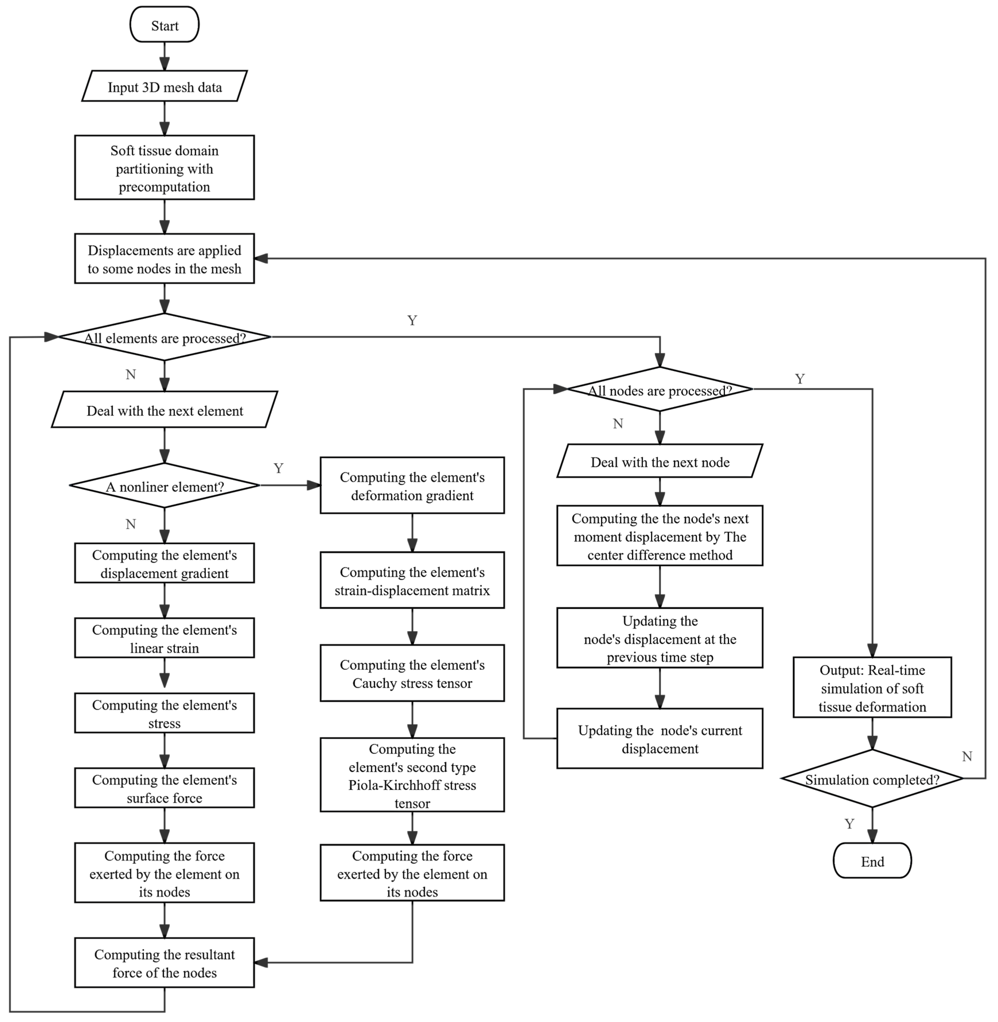
The DHD-FEA framework integrates four sequential stages: (1) soft tissue domain partitioning with precomputation, (2) subdomain-specific element stress analysis, (3) nodal resultant forces analysis, and (4) hybrid model-driven displacement resolution. Initially, the tissue geometry is partitioned into linear and nonlinear subdomains using biomechanical criteria, with tailored precomputation of domain-specific parameters (e.g., material properties and geometric invariants). A hybrid finite element methodology is selectively applied to each subdomain during the element analysis phase, deriving critical mechanical metrics—including stress tensors, strain distributions, and nodal interaction forces—through subdomain-appropriate constitutive models. Following this, nodal force integration synthesizes all element-induced force contributions at each node via vector summation, yielding the resultant force field across the tissue mesh. Finally, explicit time integration is implemented to compute dynamic nodal displacements between successive timesteps, enabling deterministic reconstruction of vertex trajectories and tissue morphodynamics. This framework achieves an optimized balance between computational tractability and biomechanical realism through adaptive domain-specific computation and hybrid numerical formulation.
The program flowchart of the DHD-FEA is shown in Figure 2.
The algorithm process is basically the same as that of the TLED algorithm. The difference lies in that during the element analysis, the DHD-FEA adopts two FEMs and will determine whether to use a linear model or a nonlinear model for the solution based on the type of element.

3.2.1. Soft Tissue Domain Partitioning with Precomputation

Soft tissue structures are computationally modeled as 3D mesh data to serve as algorithm inputs in the study. A structured spatial discretization approach is implemented that partitions the regular cuboid domain into finite elements through systematic subdivision to enable systematic algorithmic control over mesh resolution. The methodology initiates with volumetric decomposition of the bounding cuboid into uniform hexahedral elements, followed by subsequent refinement where each cubic element undergoes optimized partitioning into five tetrahedral sub-elements. This hierarchical discretization process generates a comprehensive set of finite elements and corresponding nodal coordinates to ensure both geometric regularity and computational tractability for subsequent numerical analysis (Figure 3).
The algorithm also enables precise control over the mesh density (number of elements), the geometric properties (shape and size) of individual elements, and the spatial distribution of the grid. Such programmatic adaptability provides critical flexibility for simulating soft tissue deformation to ensure biomechanical accuracy (Figure 4).
The model’s elements must be partitioned into two categories to solve soft tissue deformation using the DHD-FEA: linear and nonlinear elements. The delineation of surgical zones can become nontrivial for complex anatomical structures or specific surgical maneuvers that require meticulous consideration of mesh geometry, the proportion of nonlinear finite elements, and their spatial distribution. Consequently, scenario-specific mesh configurations must be prepared for targeted operative contexts when applying this algorithm for surgical simulation. Elements may be categorized hierarchically in the simplest implementation. For instance, a mesh comprising five hierarchical layers as illustrated in Figure 3 can be configured by designating select layers as linear elements and the remainder as nonlinear. This study assumes surgical interactions occur on the top surface of a rectangular prism-shaped soft tissue mesh. Accordingly, the upper portion of the prism is assigned nonlinear soft tissue properties while the lower elements are treated as linear.
The primary focus is on mesh element attributes and their nodal connectivity relationships in deformation computation using FEMs. Conversely, the graphics rendering pipeline prioritizes the object’s surface mesh topology. This dichotomy necessitates a data structure architecture for deformation simulation programs as schematically depicted in Figure 5.
The entire object domain is discretized into tetrahedral elements, each comprising four nodes. The simulation employs preprocessed data for computational efficiency. Specifically, the element information encompasses precomputed physical quantities from Equation (18), precomputed data tDX from Equation (7), and the initial volume of each element. Additionally, the node information includes the nodal mass, the initial position of the node, the resultant force acting on the node due to internal and external forces, the displacement at the previous time step, the current displacement, and the predicted displacement for the next time step. We assume that there is a tetrahedral unit in the current target region with nodes P 1 , P 2 , P 3 , and P 4 (as shown in Figure 6).
The tetrahedral volume is calculated as shown in Equation (1), as follows:
V = ( ( P 2 P 1 ) × ( P 3 P 1 ) ) × ( P 4 P 1 ) / 6

3.2.2. Subdomain-Specific Element Stress Analysis

The finite elements are divided into linear and nonlinear elements according to their location in the DHD-FEA method, as expressed in Equations (2) and (3).
K O O K O I K I O K I I O U O U I = R O R I
K I I N K I N K N I K N N U I U N = R I R N
O is the Operational Region, N is the Non-Operational Region, and I is the common area of the two regions. The equations of the two parts are similar, but the finite element equations are different. This section mainly describes the element stress analysis methods of linear finite elements and nonlinear finite elements.
  • The linear finite elements stress analysis method
The deformation of linear finite elements is constrained to less than 10% in this framework, enabling the use of the initial (reference) configuration to approximate the deformed geometry. The Cauchy strain tensor and Cauchy stress tensor are employed to characterize the material’s strain and stress states, respectively. Due to the fixed linear constitutive relationship between strain and stress—which remains invariant to the deformation magnitude—the linear model achieves higher computational efficiency compared to nonlinear approaches. However, this simplification compromises simulation accuracy as it neglects geometric and material nonlinearities inherent to large deformations.
A tetrahedral element with nodes P 1 , P 2 , P 3 , and P 4 has initial nodal positions x i 1 0 , x i 2 0 , x i 3 0 , and x i 4 0 and deformed positions x i 1 t , x i 2 t , x i 3 t , and x i 4 t , as illustrated in Figure 6. The displacement field must be determined throughout the element to compute the Cauchy strain tensor, which requires derivation of the displacement gradient. For an arbitrary material point within the tetrahedron, let its initial coordinate be x i 0 and deformed position be x i t . The weights governing this point’s spatial relationship to the other tetrahedral nodes remain invariant throughout the deformation process. The x i 0 and x i t of a point are calculated using Equation (4), as follows:
x i 0 = x i 2 0 x i 1 0 b 1 + x i 3 0 x i 1 0 b 2 + x i 4 0 x i 1 0 b 3
= x 1 2 0 x 1 1 0 x 1 3 0 x 1 1 0 x 1 4 0 x 1 1 0 x 2 2 0 x 2 1 0 x 2 3 0 x 2 1 0 x 2 4 0 x 2 1 0 x 3 2 0 x 3 1 0 x 3 3 0 x 3 1 0 x 3 4 0 x 3 1 0 b 1 b 2 b 3 = D X 0 b
b = ( b 1 ,   b 2 ,   b 3 ) T are the weights of a point, and D X 0 is calculated with Equation (5) as follows:
D X 0 = x 1 2 0 x 1 1 0 x 1 3 0 x 1 1 0 x 1 4 0 x 1 1 0 x 2 2 0 x 2 1 0 x 2 3 0 x 2 1 0 x 2 4 0 x 2 1 0 x 3 2 0 x 3 1 0 x 3 3 0 x 3 1 0 x 3 4 0 x 3 1 0
In the same way, x i t is calculated as follows:
x i t = x i 2 t x i 1 t b 1 + x i 3 t x i 1 t b 2 + x i 4 t x i 1 t b 3 = x 1 2 t x 1 1 t x 1 3 t x 1 1 t x 1 4 t x 1 1 t x 2 2 t x 2 1 t x 2 3 t x 2 1 t x 2 4 t x 2 1 t x 3 2 t x 3 1 t x 3 3 t x 3 1 t x 3 4 t x 3 1 t b 1 b 2 b 3 = D X t b
b = ( b 1 ,   b 2 ,   b 3 ) T are the weights of a point, and D X t is calculated using Equation (7) as follows:
D X t = x 1 2 t x 1 1 t x 1 3 t x 1 1 t x 1 4 t x 1 1 t x 2 2 t x 2 1 t x 2 3 t x 2 1 t x 2 4 t x 2 1 t x 3 2 t x 3 1 t x 3 3 t x 3 1 t x 3 4 t x 3 1 t
Finally, the position of a point after deformation is calculated as follows:
x 1 t x 2 t x 3 t = D X t D X 1 0 x 1 0 x 2 0 x 3 0 = P 0 t x 1 0 x 2 0 x 3 0
P 0 t = D X t D X 1 0 is a 3 by 3 matrix representing the mapping of any point position inside the tetrahedron before and after deformation, and the displacement of any point can be expressed as u i t = P i k 0 t x k 0 x i 0 . And since D 0 X 1 remains constant throughout the simulation process, it is feasible to pre-calculate it.
Therefore, the displacement gradient of a point is calculated using the following equation:
u i t x j 0 = x j 0 P i k 0 t x k 0 x i 0 = P i j 0 t x i 0 x j 0 = P 0 t I
where I is the identity matrix, and the Cauchy strain tensor can be expressed as follows:
ε = 1 2 P 0 t + P T 0 t 2 I
The Cauchy stress σ is obtained through the constitutive equation after calculating the Cauchy strain tensor. The Cauchy stress σ is defined as shown in Equation (11):
d f d A = σ n
where df is the force acting on an infinitesimal surface in space, dA is the area of that surface, and n is the unit normal vector to the surface.
Therefore, the resultant force acting on each face of the tetrahedral element due to stress can be obtained from Equation (12):
f = ( σ n ) A
where σ a denotes the Cauchy stress tensor, n is the unit normal vector to the triangular face of the tetrahedral element, and A represents the area of the triangular face. Since the tetrahedron is modeled as a linear finite element, the resultant surface force f can be uniformly distributed to each node of the triangular face, thereby allowing the nodal forces F ~ t exerted by the tetrahedral element on all nodes to be determined.
2.
The nonlinear finite elements stress analysis method
The nonlinear model of the DHD-FEA in the surgical area employs the TLED algorithm. Due to the substantial deformations often exhibited by soft tissues in surgical regions, linear strain tensors such as the infinitesimal (Cauchy) strain tensor are inadequate for solving such nonlinear problems. Instead, the Green–Lagrange strain tensor is adopted as the nonlinear strain measure and the stress tensor is correspondingly replaced by the Second Piola–Kirchhoff stress tensor. Furthermore, the constitutive relationship between stress and strain in these materials is not fixed. A simplified yet effective nonlinear framework for modeling such behavior is the hyperelastic model, where many biological soft tissues can be approximated as hyperelastic materials characterized by strain energy density functions. The nodal forces exerted by nonlinear elements on their corresponding nodes can be calculated using Equation (13).
F ~ t = V 0 B L T 0 t S ^ 0 t d V 0
S ^ 0 t = S 11 0 t   S 22 0 t   S 33 0 t   S 12 0 t   S 23 0 t   S 13 0 t is the vector form of the second Piola–Kirchhoff stress, B L T 0 t is the strain–displacement matrix, and V 0 is the initial volume of an element. This equation performs force analysis at the element level, with all variable values obtainable from the local information of the element.
The neo-Hookean model is employed to solve for the stress tensor S ^ 0 t . The stress components S ^ 0 t are derived by differentiating the neo-Hookean strain energy function W with respect to the Green strain tensor [23,24]. And the equation is as follows:
S i j 0 t = μ δ i j C i j 1 0 t + λ J t J t 1 C i j 1 0 t
where C 0 t is the right Cauchy–Green deformation tensor. And C 0 t is calculated as follows:
C 0 t = X T 0 t X 0 t
As the strain–displacement matrix B L T 0 t is related to the geometry of the element, it changes with the geometry of the element. Because a tetrahedron contains four nodes, B L 0 t can be represented as a set of its submatrices:
B L 0 t = B L 0 0 t B L 1 0 t B L 2 0 t B L 3 0 t
B L ( i ) 0 t is the I-th node of the corresponding element of the I-th submatrix of B L 0 t . And B L ( i ) 0 t is calculated as follows:
B L i 0 t = B L 0 i 0 X T 0 t
X T 0 t is the deformation gradient of the element. And B L 0 i 0 t is calculated using Equation (18).
B L 0 i 0 = h i x 0 0 0 0 h i y 0 0 0 0 h i z 0 h i y 0 h i x 0 0 0 h i z 0 h i y 0 h i z 0 0 h i x 0
To solve for B L 0 ( i ) 0 t , it is necessary to compute the derivatives of the shape functions with respect to the spatial coordinates h i x 0 , h i y 0 , and h i z 0 . And the spatial derivatives of shape functions are typically calculated using the isoparametric finite element formulation. The core principle of the isoparametric finite element formulation lies in relating the displacement at any point within an element to the nodal displacements through shape functions. The shape function h i at the four nodes P 1 , P 2 , P 3 , and P 4 can be expressed as h i ( r ,   s ,   t ) in a tetrahedral isoparametric element, where the isoparametric coordinates r, s, and t are defined in the range of [−1, 1], as shown in Equation (19):
h 1 = 1 8 ( 1 r ) ( 1 s ) ( 1 t ) h 2 = 1 8 ( 1 + r ) ( 1 s ) ( 1 t ) h 3 = 1 4 ( 1 + s ) ( 1 t ) h 4 = 1 2 ( 1 + t )
where i denotes the local index of the corresponding vertex within the element.
The relationship between the derivatives of the shape functions according to the rules of partial differentiation and the isoparametric coordinates is given in Equation (20).
h i r = h i x 0 1 x 0 1 r + h i x 0 2 x 0 2 r + h i x 0 3 x 0 3 r h i s = h i x 0 1 x 0 1 s + h i x 0 2 x 0 2 s + h i x 0 3 x 0 3 s h i t = h i x 0 1 x 0 1 t + h i x 0 2 x 0 2 t + h i x 0 3 x 0 3 t
Equation (20) derives the relationship between the partial derivatives of the shape functions with respect to the isoparametric coordinates and the partial derivatives of the shape functions with respect to the physical coordinates, as well as the partial derivatives of the physical coordinates with respect to the isoparametric coordinates, using the chain rule. Through a series of identity transformations, Equation (21) is obtained.
h i r h i s h i t = x 0 1 r x 0 2 r x 0 3 r x 0 1 s x 0 2 s x 0 3 s x 0 1 t x 0 2 t x 0 3 t h i x 0 1 h i x 0 2 h i x 0 3 = h i r x 0 1 i h i r x 0 2 i h i r x 0 3 i h i s x 0 1 i h i s x 0 2 i h i s x 0 3 i h i t x 0 1 i h i t x 0 2 i h i t x 0 3 i h i x 0 1 h i x 0 2 h i x 0 3 = h 1 r h 2 r h 3 r h 4 r h 1 s h 2 s h 3 s h 4 s h 1 t h 2 t h 3 t h 4 t x 0 1 1 x 0 2 1 x 0 3 1 x 0 1 2 x 0 2 2 x 0 3 2 x 0 1 3 x 0 2 3 x 0 3 3 x 0 1 4 x 0 2 4 x 0 3 4 h i x 0 1 h i x 0 2 h i x 0 3
Therefore, the spatial derivatives of the shape functions (with respect to physical coordinates) can be computed, as shown in Equation (22):
h i x 0 1 h i x 0 2 h i x 0 3 = h 1 r h 2 r h 3 r h 4 r h 1 s h 2 s h 3 s h 4 s h 1 t h 2 t h 3 t h 4 t x 1 1 0 x 2 1 0 x 3 1 0 x 1 2 0 x 2 2 0 x 3 2 0 x 1 3 0 x 2 3 0 x 3 3 0 x 1 4 0 x 2 4 0 x 3 4 0 1 h i r h i s h i t
h i r , h i s , and h i t represent the derivatives of the shape functions with respect to the isoparametric coordinates in an isoparametric element. Since the isoparametric coordinates of points within each element remain invariant, the derivative values of the shape functions at the integration points are constant throughout the simulation.
For each tetrahedral element, the initial positions of its four nodes are x i 1 0 , x i 2 0 , x i 3 0 , and x i 4 0 . Since these positions remain invariant throughout the deformation simulation, the spatial derivatives of the shape functions computed via Equation (22) are also constant during the entire deformation process. Thus, the B L 0 i 0 matrix can be computed using Equation (18), and subsequently, the strain–displacement matrix B L T 0 t for the element can be obtained via Equation (16). With these matrices, the nonlinear internal forces acting on the element’s nodes can be further determined. Crucially, the B L 0 i 0 matrix remains invariant throughout the entire deformation simulation, yet its computation is computationally intensive. Therefore, the B L 0 i 0 matrix for each element is precomputed during the preprocessing stage, and the pre-computed data are directly reused in real-time simulations to significantly accelerate the deformation computation.
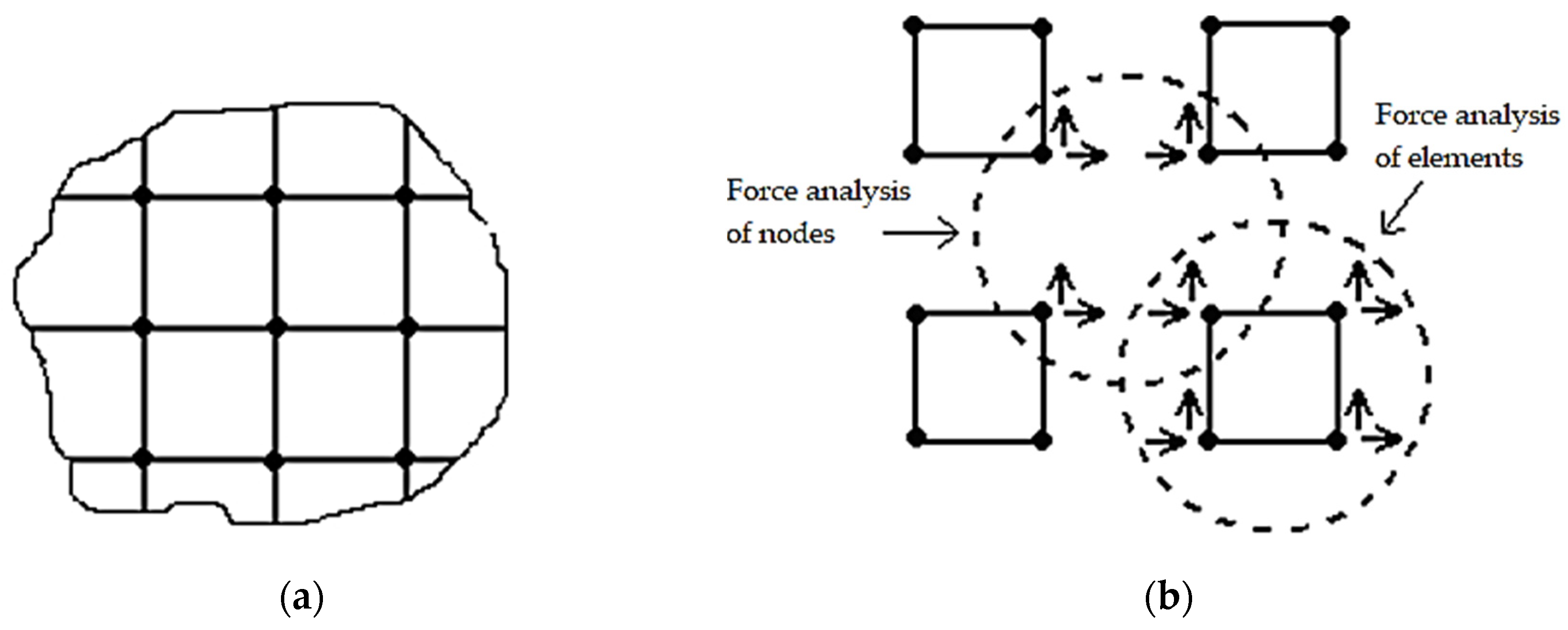
Following the mechanical analysis of linear and nonlinear zonal elements, it is necessary to apply all resultant forces to the interface nodes. The interfacial nodes connecting both zones, referred to as intermediate nodes, exhibit hybrid connectivity with both nonlinear and linear elements. Conventional Equations (2) and (3) typically require independent computation of these intermediate nodes followed by simultaneous solution of the coupled equation systems. However, the proposed algorithm eliminates the need for global stiffness matrix assembly, thereby enabling direct integration of intermediate nodes through a streamlined computational process. The forces exerted by each element on its connected nodes are computed without nodal type restrictions during element-level analysis to ensure comprehensive force transmission to all nodes—whether in nonlinear zones, linear zones, or intermediate positions. Subsequent nodal force analysis inherently incorporates all nodal points by calculating the resultant forces acting on each node through superposition of contributions from adjacent elements. This methodology naturally accommodates intermediate nodes within the standard computational framework, achieving systematic force equilibrium without necessitating special treatment for interfacial nodes.

3.2.3. Nodal Resultant Forces Analysis

The DHD-FEA determined the nodal force vectors F ~ t exerted by tetrahedral elements on their corresponding nodes following the elemental stress analysis. The subsequent computational phase necessitates the evaluation of the resultant force at each node v through systematic superposition of contributions from all topologically connected elements. Let F t e denote the force exerted by an incident element e connected to the node for each nodal point within the discretized mesh. The resultant force F v acting on the node due to all incident elements is computed through vector superposition as prescribed in Equation (23):
F v = e F e t
The total resultant force is computed as R v F v when external forces R v (e.g., applied nodal loads, boundary tractions, or body forces) act on node v.
The displacement field within an element is approximated through nodal displacement interpolation in the DHD-FEA, while distributed external forces and internal interactions between adjacent elements are consistently acting as nodal forces. This framework enables the application of Newtonian mechanics for nodal equilibrium analysis. For static systems, nodes remain in a stationary state governed by the equilibrium relationship expressed in Equation (24).
R v = F v = e F t e
For dynamic systems without damping effects, the nodal dynamic equilibrium equation is formulated as
m v u ¨ v + F v = R v
where m v is the mass of a node, and u v is the displacement of the node. The nodal acceleration u ¨ v is the second derivative of the nodal displacement u v with respect to time. F v is the force exerted by the unit pair on the node, and R v is the resultant force of the external forces acting on the node. For the nodes with damping effect, their dynamic equilibrium equations are as shown in Equation (26).
m v u ¨ v + d v u ˙ v + F v = R v
The damping term d v u ˙ v is added in the above equation, Equation (26). And d v represents the damping factor of the node, and the node velocity u ˙ v is the first derivative of the node displacement u v with respect to time.

3.2.4. Hybrid Model-Driven Displacement Resolution

All physical quantities remain independent of time in static systems. Static equilibrium equations K U = R can also be applied to quasi-static scenarios. The system states evolve temporally, but at a sufficiently slow rate that inertial and damping effects become negligible in such scenarios. These formulations are applicable to analyses including foundation settlement and dam impoundment. However, their suitability diminishes in surgical contexts involving tissue deformation and incision operations, where rapid state variations occur—for instance, the viscoelastic rebound and oscillation of organs following instrument indentation. When temporal displacement variations exhibit significant rates, necessitating the consideration of inertial effects, dynamic system formulations become imperative. In such systems, acceleration terms manifest explicitly in the governing equations, accompanied by velocity-dependent damping effects. Compared to static systems, displacement variables attain heightened significance in dynamic analyses. The fundamental governing equations of dynamics derive from force equilibrium principles rooted in Newtonian mechanics, incorporating both inertial and dissipative forces.
An exact solution can typically be obtained in static analysis. However, achieving an exact solution is significantly more challenging due to the need to account for material distribution and damping effects in dynamic analysis [25]. It is necessary to generate at least a mass matrix to complement the stiffness matrix in dynamic finite element analysis. The assembly procedures for the mass matrix M and stiffness matrix K can be executed concurrently within finite element frameworks. Element-level mass matrices are initially formulated in local coordinate systems before undergoing coordinate transformation to the global system that mirrors the assembly methodology employed for the global stiffness matrix. A fundamental distinction between these matrices lies in the diagonalization capability of the mass matrix via direct lumping techniques. This diagonalization confers critical computational advantages: (1) the inversion of diagonal matrices requires substantially fewer operations compared to full matrices, and (2) the diagonal structure enables explicit time integration schemes at the element level without coupled equation solutions. Consequently, mass lumping significantly optimizes computational efficiency in dynamic simulations.
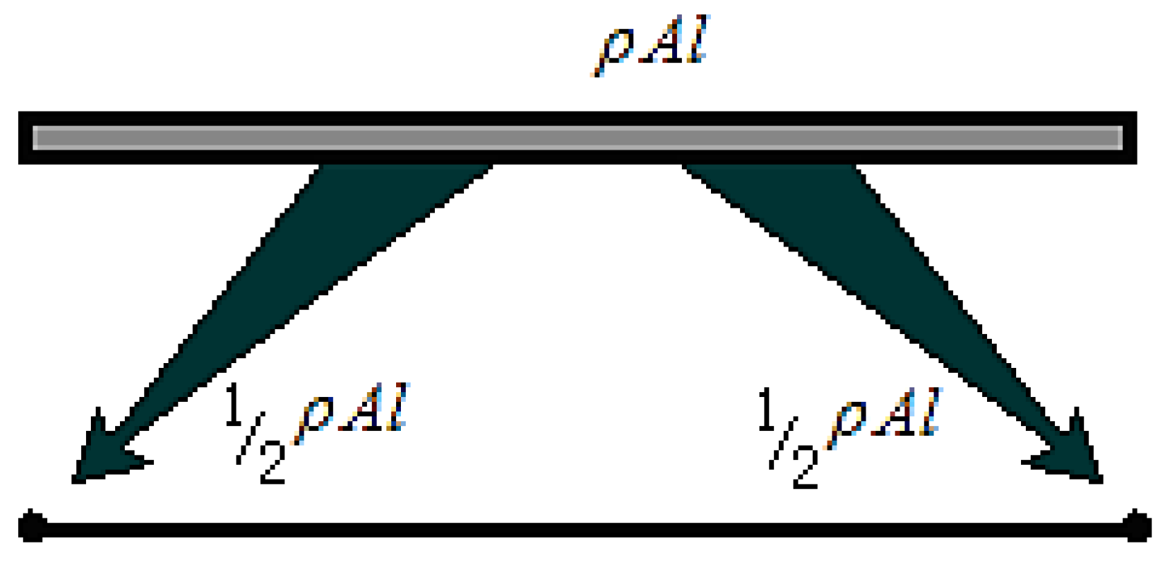
The objective of direct mass lumping (DML) is to generate a diagonally lumped mass matrix (DLMM) for dynamic systems. This technique allocates the total mass of element e to its nodal degrees of freedom by directly distributing mass contributions to individual nodes, thereby eliminating off-diagonal coupling terms associated with inter-nodal interactions. The simplest illustration of direct mass lumping involves a two-node prismatic bar element with length l, uniform cross-sectional area A, and mass density ρ , as depicted in Figure 7.
The total mass ρ V of a tetrahedral element (where ρ is material density and V denotes element volume) is distributed to its four nodes using the mass lumping method as illustrated in Figure 8.
The finite element mass matrix is transformed into a diagonal matrix via the direct mass lumping procedure, where elemental mass is redistributed to nodal degrees of freedom while preserving total mass conservation. Under the proportional damping assumption ( D = α M , where α is a material-dependent constant), the damping matrix inherits the diagonal structure from the lumped mass matrix. This formulation allows the stiffness term K ( U ) U to be expressed in the decoupled form of Equation (27):
K ( U ) U = F ( U ) = e F ~ ( e )
e is the elements in the set, and F ~ ( e ) is the force of an element on the node. Equation (27) describes that the internal forces acting on each node in a structural system can be calculated through the assembly of the global stiffness matrix followed by its multiplication with the nodal displacement vector. Alternatively, the second methodology involves conducting stress analysis at the element level, where individual unit contributions are resolved through constitutive relationships.
The diagonal configuration of both mass matrix M and damping matrix D indicates that nonzero elements exclusively populate their main diagonals, while off-diagonal entries remain 0. This structural property ensures that the mass and damping characteristics of each node operate independently, with no cross-coupling effects between distinct nodes in the system. The dynamic equilibrium in Equation (28), governing node I, incorporates the combined effects of internal stress-induced resultant force F i , its mass M i i , damping coefficient D i i , instantaneous displacement U i , and externally applied load R i .
M i i U ¨ i + D i i U ˙ i + F i = R i
The integration of governing equations with the inherent diagonal properties of mass and damping matrices establishes a hierarchical computational framework for deformation simulation. This methodology enables multi-level analysis by leveraging element-specific stress–strain relationships and nodal dynamic equilibrium principles, ensuring that localized force interactions are systematically resolved while maintaining global system compatibility.
The DHD-FEA methodology addresses the challenge of real-time tissue/organ deformation simulation in surgical contexts by strategically partitioning computational domains: nonlinear FEM formulations govern the surgical region to capture complex biomechanical responses, while linear FEM approximations are applied to non-surgical zones to reduce computational overhead. This multi-resolution framework optimizes computational resource allocation while maintaining physiological fidelity. Additionally, domain-specific numerical integration strategies are implemented to efficiently solve equilibrium equations, enabling stable convergence under large deformation scenarios. The temporal discretization of governing equations can be implemented through explicit or implicit integration schemes, each offering distinct computational trade-offs [22]. But implicit integration methods maintain unconditional stability but require iterative solutions to couple nonlinear algebraic systems, resulting in significant computational demands. In contrast, explicit schemes achieve computational efficiency through non-iterative formulations, directly advancing solutions without solving coupled equations, a feature particularly advantageous for dynamic systems governed by strict time-step constraints.
The central difference method is an explicit integration scheme designed to approximate solutions for second-order differential equations [21]. This approach is employed to solve Equation (28) in the DHD-FEA, leveraging its capability to compute state variables at subsequent time steps based entirely on current dynamic conditions. The temporal progression follows discrete time intervals governed by a fixed time step in computational dynamics simulations. When initializing a simulation at t = 0 with a defined temporal resolution Δ t , the current state at time t inherently determines the subsequent time increment as t + Δ t through explicit temporal discretization. Within the framework of Equation (28), the displacement vector U i constitutes the primary unknown requiring numerical resolution. Concurrently, all other system parameters including but not limited to velocity vectors, acceleration profiles, and environmental constraints become computationally accessible through explicit state transitions during each stepwise calculation. This deterministic progression ensures temporal causality while maintaining numerical stability through fixed-interval updates.
The central difference method employs iterative temporal discretization to determine the unknown displacement function U t + Δ t i at subsequent time instant t + Δ t , where temporal superscripts systematically denote measurement instances as illustrated in Figure 9. This explicit algorithm calculates first-order derivatives at time t through symmetric differencing principles, utilizing displacement states from adjacent time intervals to construct velocity approximations.
Therefore, the first- and second-order temporal derivatives of displacement function U i at time t are formulated as follows:
U ˙ i t = U t + Δ t i U t Δ t i 2 Δ t
U ¨ i t = U t + Δ t i 2 U t i + U t Δ t i Δ t 2
U ¨ i t is the second derivative at time t. The nodal equilibrium equations are derived by substituting Equations (29) and (30) into Equation (28), resulting in the governing formulation expressed as Equation (31).
M i i U t + Δ t i 2 U t i + U t Δ t i Δ t 2 + D i i U t + Δ t i U t Δ t i 2 Δ t + F t i = R t i
The governing equations are algebraically transformed through identity operations, ultimately yielding the consolidated formulation expressed as Equation (32).
U t + Δ t i = 2 Δ t 3 2 M i i Δ t + D i i Δ t 2 R t i F t i + 4 M i i Δ t 2 M i i Δ t + D i i Δ t 2 U t i 2 M i i Δ t D i i Δ t 2 2 M i i Δ t + D i i Δ t 2 U t Δ t i
And Equation (33) is obtained by simplifying Equation (32).
U t + Δ t i = A i R t i F t i + B i U t i C i U t Δ t i
Equation (33) provides an efficient computational framework for determining nodal displacements at subsequent time steps in the DHD-FEA. This enables accurate reconstruction of object deformation characteristics through systematic time-domain integration.

3.3. Analysis of Elasticity

The implicit integration method exhibits unconditional stability in numerical simulations, while the explicit integration method is only conditionally stable. Numerical convergence requires the time step Δ t to remain strictly below the critical threshold Δ t c r , which governs the maximum allowable temporal resolution in dynamic analyses for explicit schemes. Δ t c r can be systematically determined through material properties and discretization parameters in linear elastic systems [26,27,28].
Δ t c r = L e c
L e represents the minimum characteristic element length within the element set, and c denotes the longitudinal wave propagation speed of the material, both of which can be systematically determined through material properties and discretization parameters.
c = E ( 1 ν ) ρ ( 1 + ν ) ( 1 2 ν )
E represents Young’s modulus (characterizing material stiffness), v denotes Poisson’s ratio (quantifying lateral strain response), and ρ indicates the material density (mass per unit volume). This equation adheres to the fundamental principles of dynamic time-step control in finite element analysis, where spatial discretization scales and wave propagation characteristics govern numerical stability criteria.
Employing reduced critical time steps becomes imperative compared to linear analyses in both material and geometric nonlinear analyses. This necessity arises from dynamic variations in wave propagation characteristics, where structural configuration changes during deformation processes typically amplify effective wave velocities. The temporal resolution can be systematically optimized through characteristic time parameter Δ t c r , which adaptively accounts for evolving material states and geometric configurations while maintaining numerical stability.
While explicit integration methods maintain conditional stability, their computational advantage becomes particularly pronounced in simulating soft biological tissues. The critical time step demonstrates inverse proportionality to material stiffness, enabling surprisingly large stable increments when modeling low-Young’s-modulus materials like visceral organs.

4. Results

4.1. The Simulation Efficacy of DHD-FEA Model

The soft tissue model was simulated through interactive tools and liver data [29] in the research. The model was meshed through the finite element software ABAQUS to generate the set of FEs. This study implemented simulation models for both the DHD-FEA model and the TLED deformation algorithm on a standard PC to evaluate the real-time performance of the hybrid finite element model. A comparative analysis was conducted between the two models in terms of their real-time performance. The nonlinear soft tissue constitutive relationship was modeled using the neo-Hookean model, with a Young’s modulus of 5000 Pa, a Poisson’s ratio of 0.35, and a material density of 1000 kg/m³ in all simulations. The results of the simulations are presented in Figure 10.

4.2. The Algorithmic Performance Evaluation of DHD-FEA Model

For instance, since the refresh rate of the graphics card is fixed, the frame rate of the simulated PC in this article is 75 Hz. A larger grid scale is adopted in this simulation to reduce the frame rate to a range that is convenient for comparison to visually observe the performance differences between the two algorithms. Otherwise, the frame rate of the algorithm will be limited to the refresh rate of the graphics card when the grid is small. The deformation simulation of the soft tissue grid containing 3564 nodes and 14,450 elements is carried out using the DHD-FEA in the simulation, and the relationship between the proportion of linear elements and the simulation frame rate is investigated. The frame rate changes obtained from the simulation are shown in Table 1.
The DHD-FEA is superior in terms of computational efficiencies compared with to TLED algorithm, as shown in Table 1. However, the efficiency advantage of this algorithm comes at a cost. The later error analysis reveals that as efficiency increases, error also gradually increases.
By applying different displacements to certain nodes of the mesh and gradually increasing the proportion of linear finite elements in the mesh in the simulation, the differences between the simulation results of the DHD-FEA and the TLED algorithm under the corresponding conditions are verified. The simulation scenario is shown in Figure 11.
The ratio of linear elements to nonlinear elements in the DHD-FEA is denoted as r. The TLED algorithm also uses the same mesh and applies the same displacement. The difference is that all the elements are nonlinear in the meshes processed using the TLED algorithm. Therefore, the TLED algorithm can be regarded as a special case of the DHD-FEA model, with r = 0. A downward displacement is applied to the soft tissue at the center position of the upper surface of the cuboid. The upper surface will then have a depression. Figure 10 shows the error analysis simulation scenario for r = 30%.
It is necessary to measure the “distance” between the meshes of the deformed shapes processed using the two algorithms in order to measure the accuracy difference between the DHD-FEA and the TLED algorithm. The shape of the deformed meshes is directly related to the positions of the mesh nodes. The difference in deformation of objects with the same initial positions can be measured by the difference in corresponding node displacements, which is defined as the modulus of the difference in displacements of corresponding nodes. We use the average difference to measure the computational error of the DHD-FEA and the TLED algorithm. Since this algorithm takes into account dynamic systems with inertia and damping, the deformation of the model has temporal sequence. Two algorithms are used to apply displacements to the surface of a cuboid at the initial moment, and the average error is calculated after 1000 iterations.
The average errors under the conditions of linear element ratios of 10%, 20%, 30%, and 40% are tested, respectively, when a displacement vector with a length of 0.6 is applied to the upper surface of the cuboid, as shown in Table 2.
Table 2 indicates that as the proportion of linear elements within the grid increases, the error of the algorithm gradually increases. This is mainly because as the displacement is applied, the elements within the grid deform. This will lead to an increase in error if there are linear elements at this time and they undergo large deformations. Therefore, the average error of the algorithm will also increase as the number of linear elements in the model increases.
The average errors under conditions of linear element ratios of 10%, 20%, 30%, and 40% when a displacement of 1.0 is applied to the upper surface of the cuboid are shown in Table 3, based on the simulation results.
It can be seen from the comparative analysis of the simulation results in Table 2 and Table 3 that, in the case of the same proportion of linear FEs, as the applied displacement increases (from 0.6 to 1.0), the error of the algorithm also increases accordingly. This is mainly because the increase in displacement leads to an increase in the deformation of the rectangular soft tissue, causing more elements to undergo greater deformation. Therefore, the error of the model also increases accordingly.

4.3. The Simulation Effect and Analysis in the Surgical Area

During the simulation process, several nodes at the left end of the soft tissue with an initial shape of a cuboid are fixed, and the remaining parts hang freely. A line segment representing the scalpel is used to cut the middle part of the soft tissue during the falling process.
As the cutting proceeds, the topological structure of the mesh is constantly updated in the simulation of the real-time cutting method based on nonlinear finite elements. Meanwhile, the algorithm efficiently generates pre-computed data for the newly generated elements. In this way, the algorithm transitions to the finite element deformation stage. At this stage, the algorithm conducts force analysis on each element to solve the force exerted by each element on its nodes. Then, it performs force analysis on each node to find the resultant force acting on the nodes. Finally, it uses explicit time integration to solve for the positions of each node of the soft tissue at the next moment to complete one update of the scene. Meanwhile, we compared this method with the adaptive FEM [21], and the visual effect is shown in the following Figure 12.
The soft tissue is cut through as the scalpel moves. The change in topology affects the force state of the entire soft tissue. Subsequently, the tissue on the left side of the incision slightly ascends, while the tissue on the right side of the incision descends at an accelerated rate. Eventually, the incision continues to expand under the effect of gravity. As the incision opens and the strain–stress in some units gradually increases, a new balance is slowly established. The soft tissue will eventually tend to be stationary, with an internal damping effect of the soft tissue, as shown in Figure 12a.
Figure 12b shows the cutting visual effect of the adaptive finite element algorithm. The units cut by the scalpel are directly removed during the cutting process while the DHD-FEA processes the topological structure of the mesh instead of directly removing the cutting units. Thus, the incision after cutting in Figure 12a appears relatively smooth, and the visual effect is better than that in Figure 12b.

5. Discussion

Computational efficiency will keep improving while calculation accuracy will gradually decrease as the number of linear elements in the mixed FEM increases. The error will also increase accordingly with the greater displacement applied to the upper surface of the soft tissue. This is determined by the characteristics of the linear FEM. Because the linear FEM is only suitable for small deformation situations, increasing the applied displacement will also increase the degree of object deformation, and thus, the error will also increase. The simulation accuracy and efficiency of the DHD-FEA are related to the displacement degree of nodes in the mesh and the proportion of linear elements in the mesh. Therefore, this algorithm can adjust computational efficiency and accuracy according to specific simulation requirements to meet the needs of different simulations, which is more flexible than the complete linear FEM or the complete nonlinear FEM.

6. Conclusions

We propose a relatively flexible DHD-FEA model to balance the accuracy and real-time performance of soft tissue deformation simulation. A more accurate nonlinear finite element method is adopted to improve accuracy for the surgical area of soft tissues during operation. While a more efficient linear finite element method is used to enhance the real-time performance for soft tissues in the non-surgical area. Furthermore, explicit integration is used to simulate dynamic surgical scenarios and solves the problem of pre-computation failure of the finite element in the surgical area. Finally, the experiments show that the simulation accuracy of this algorithm is higher than that of the complete linear finite element method, and the simulation real-time performance is higher than that of the complete nonlinear finite element method.
However, this method still needs further improvement, which is also part of our research plan. Firstly, the neo-Hookean model adopted in this paper is only a simple model in the nonlinear constitutive equation, while the constitutive equations of real soft tissues are much more complex, such as viscoelasticity, plasticity, etc. The efficient implementation of these models requires further research. Secondly, the currently implemented deformation algorithms have not been verified for authenticity. Only an accurate deformation algorithm can correctly predict the effect of the corresponding surgical operation. Therefore, the verification of algorithm accuracy is an important follow-up research topic. Finally, the nonlinear FEM adopted by this method in the surgical area requires further attention to the topological update algorithm of the finite element mesh and the maintenance and real-time performance of the calculated data during the cutting process in the study of real-time cutting simulation of human soft tissues.

Author Contributions

Conceptualization, L.G. and X.G.; methodology, L.G. and X.G.; software, L.G.; validation, L.G., X.G., and F.L.; data curation, X.G.; writing—original draft preparation, L.G.; writing—review and editing, L.G. and F.L.; visualization, L.G.; supervision, X.G.; project administration, L.G.; funding acquisition, F.L. All authors have read and agreed to the published version of the manuscript.

Funding

This research was funded by the National Natural Science Foundation of China, grant number 62003004, and the “Developing Applications for the Cloud”, Research-Oriented Teaching Model Course for Undergraduate Institutions in Henan Province, number Jiao-Gao [2024] 403.

Data Availability Statement

The data presented in this study are available on request from the corresponding author.

Conflicts of Interest

Author Xin Guo was employed by the Institution Heibei Oriental College. The remaining authors declare that the research was conducted in the absence of any commercial or financial relationships that could be construed as a potential conflict of interest.

Abbreviations

DHD-FEADual-Mode Hybrid Dynamics Finite Element Algorithm
FEMFinite element method
FEFinite element

References

  1. Gladilin, E.; Zachow, S. On constitutive modeling of soft tissue for the long-term prediction of cranio-maxillofacial surgery outcome. Int. Congr. Ser. 2003, 22, 343–348. [Google Scholar] [CrossRef]
  2. Meier, U.; Lopez, O.; Monserrat, C.; Juan, M.C.; Alcaniz, M. Real-time deformable models for surgery simulation: A survey. Comput. Methods Programs Biomed. 2005, 77, 223–231. [Google Scholar] [CrossRef] [PubMed]
  3. Jing, M.J.; Cui, Z.X.; Fu, H.; Chen, X.J. Real-Time Deformation Simulation of Kidney Surgery Based on Virtual Reality. J. Shanghai Jiaotong Univ. (Sci.) 2021, 26, 290–297. [Google Scholar] [CrossRef]
  4. Picinbono, G.; Hervé Delingette; Ayache, N. Real-Time Large Displacement Elasticity for Surgery Simulation: Non-Linear Tensor-Mass Model. Springer-Verlag 2000, 1935, 643–652. [Google Scholar]
  5. Chen, F.; Gu, L.; Huang, P.; Zhang, J.; Xu, J. Soft Tissue Modeling using Nonlinear Mass Spring and Simplified Medial Reprsentation. In Proceedings of the 29th Annual International Conference of the IEEE Engineering in Medicine and Biology Society, Lyon, France, 22–26 August 2007; pp. 5083–5086. [Google Scholar]
  6. Zhu, B.; Gu, L. A hybrid deformable model for real-time surgical simulation. Comput. Med. Imaging Graph. 2012, 36, 356–365. [Google Scholar] [CrossRef] [PubMed]
  7. Patete, P.; Iaconoa, M.I.; Spadea, M.F.; Trecate, G.; Vergnaghi, D.; Mainardi, L.M.; Baroni, G. A multi-tissue mass-spring model for computer assisted breast surgery. Med. Eng. Phys. 2013, 35, 47–53. [Google Scholar] [CrossRef]
  8. Duan, Y.; Huang, W.; Chang, H.; Chen, W.; Zhuo, J.; Teo, S.K.; Su, Y.; Chui, C.K.; Chang, S. Preserved Mass-Spring Model with Novel Con- straints for Soft Tissue Deformation. IEEE J. Biomed. Health Inform. 2016, 20, 268–280. [Google Scholar] [CrossRef]
  9. Zhang, J.; Zhong, Y.; Smith, J.; Gu, C. Neural dynamics-based Poisson propagation for deformable modelling. Neural Comput. Applic 2019, 31, 1091–1101. [Google Scholar] [CrossRef]
  10. Bourantas, G.; Zwick, B.F.; Joldes, G.R.; Wittek, A.; Miller, K. Simple and robust element-free Galerkin method with almost interpolating shape functions for finite deformation elasticity. Appl. Math. Model. 2021, 96, 284–303. [Google Scholar] [CrossRef]
  11. Fahmy, M.A. Boundary element modeling and simulation of biothermomechanical behavior in anisotropic laser-induced tissue hyperthermia. Eng. Anal. Bound. Elem. 2019, 101, 156–164. [Google Scholar] [CrossRef]
  12. Fahmy, M.A. A new LRBFCM-GBEM modeling algorithm for general solution of time fractional-order dual phase lag bioheat transfer problems in functionally graded tissues. Numer. Heat Transf. 2019, 75, 616–626. [Google Scholar] [CrossRef]
  13. Fahmy, M.; Shaw, S.; Mondal, S.; Abouelregal, A.E.; Lotfy, K.; Kudinov, I.A.; Soliman, A.H. Boundary element modeling for simulation and optimization of three-temperature anisotropic micropolar magneto-thermoviscoelastic problems in porous smart structures using NURBS and genetic algorithm. Sustain. Mater. Struct. Syst. 2021, 42, 29. [Google Scholar] [CrossRef]
  14. Wu, W.; Heng, P. An improved scheme of an interactive finite element model for 3D soft-tissue cutting and deformation. Vis. Comput. 2005, 21, 707–716. [Google Scholar] [CrossRef]
  15. Ei-Said, S.A.; Atta, H.M.A.; Hassanien, A.E. Interactive soft tissue modelling for virtual reality surgery simulation and planning. Int. J. Comput. Aided Eng. Technol. 2017, 9, 38–61. [Google Scholar] [CrossRef]
  16. Liu, Y.; Kerdok, A.E.; Howe, R.D. A Nonlinear Finite Element Model of Soft Tissue Indentation. In Medical Simulation. ISMS 2004; Cotin, S., Metaxas, D., Eds.; Lecture Notes in Computer Science; Springer: Berlin/Heidelberg, Germany, 2004; Volume 3078. [Google Scholar] [CrossRef]
  17. Rong, F.; Michael, S. Simulation of planar soft tissues using a structural constitutive model: Finite element implementation and validation. J. Biomech. 2014, 47, 2043–2054. [Google Scholar]
  18. Xie, H.; Song, J.; Zhong, Y.; Li, J.; Gu, C.; Choi, K.-S. Extended Kalman Filter Nonlinear Finite Element Method for Nonlinear Soft Tissue Deformation. Comput. Methods Programs Biomed. 2021, 200, 105828. [Google Scholar] [CrossRef]
  19. Wu, W.; Heng, P.A. A hybrid condensed finite element model with GPU acceleration for interactive 3D soft tissue cutting. Comput. Animat. Virtual Worlds 2004, 15, 219–227. [Google Scholar] [CrossRef]
  20. Zhong, H.; Wachowiak, M.P.; Peters, T.M. Adaptive finite element technique for cutting in surgical simulation (Cum Laude Poster Award). Proc. SPIE 2005, 5744, 604–611. [Google Scholar] [CrossRef]
  21. Taylor, Z.A.; Comas, O.; Cheng, M.; Passenger, J.; Hawkes, D.; Atkinson, D.; Ourselin, S. On modelling of anisotropic viscoelasticity for soft tissue simulation: Numerical solution and GPU execution. Med. Image Anal. 2009, 13, 234–244. [Google Scholar] [CrossRef]
  22. Satake, U.; Senda, R.; Sambe, R.; Enomoto, T. Investigation of biological tissue cutting for minimal tissue damage using finite element simulation. Procedia CIRP 2025, 133, 495–500. [Google Scholar] [CrossRef]
  23. Wang, S.; Wang, C.; Cai, Y.; Li, G. A novel parallel finite element procedure for nonlinear dynamic problems using GPU and mixed-precision algorithm. Eng. Comput. 2020, 37, 2193–2211. [Google Scholar] [CrossRef]
  24. Simpson, B.; Zhu, M.; Seki, A.; Scott, M. Challenges in GPU-Accelerated Nonlinear Dynamic Analysis for Structural Systems. J. Struct. Eng. 2023, 149, 04022253. [Google Scholar] [CrossRef]
  25. Saini, S.; Moger, N.M.; Kumar, M.; Sarkar, S.; Mittal, S.; Ifthekar, S.; Ahuja, K.; Singh, I.V.; Kandwal, P. Biomechanical analysis of Instrumented decompression and Interbody fusion procedures in Lumbar spine: A finite element analysis study. Med. Biol. Eng. Comput. 2023, 61, 1875–1886. [Google Scholar] [CrossRef] [PubMed]
  26. Sabet, F.A.; Koric, S.; Idkaidek, A; Jasiuk, I. High-Performance Computing Comparison of Implicit and Explicit Nonlinear Finite Element Simulations of Trabecular Bone. Comput. Methods Programs Biomed. 2021, 200, 105870. [Google Scholar] [CrossRef] [PubMed]
  27. Wang, G.; Liu, J.; Lian, T.; Sun, Y.; Chen, X.; Todo, M.; Osaka, A. Distribution and propagation of stress and strain in cube honeycombs as trabecular bone substitutes: Finite element model analysis. J. Mech. Behav. Biomed. Mater. 2024, 159, 106647. [Google Scholar] [CrossRef] [PubMed]
  28. Schwiedrzik, J.; Gross, T.; Bina, M.; Pretterklieber, M.; Zysset, P.; Pahr, D. Experimental validation of a nonlinear FE model based on cohesive-frictional plasticity for trabecular bone. Int. J. Numer. Methods Biomed. Eng. 2015, 32, e02739. [Google Scholar] [CrossRef]
  29. Prieto-Vázquez, A.Y.; Cuautle-Estrada, A.; Grave-Capistrán, M.A.; Ramírez, O.; Torres-SanMiguel, C.R. Fractal Analysis and FEM Assessment of Soft Tissue Affected by Fibrosis. Fractal Fract. 2023, 7, 661. [Google Scholar] [CrossRef]
Figure 1. Force analysis of the FEM. (a) Partial elements of continuum mechanics. It can be seen that continuum mechanics are divided into several elements. The type of element is rectangular. And other types of elements can also be used, such as triangles, cuboids, etc. Elements are connected to each other through nodes, and each node is linked to several elements. Each connected element will exert a force on that node. (b) A finite element force analysis process. The dotted circle represents the area of concern for the analysis. Firstly, conduct the force analysis of the elements to calculate the force exerted by each element on its nodes. Then, carry out the force analysis of the nodes to analyze the resultant force acting on each node. The arrows around each node indicate the direction of the interaction forces between the nodes.
Symmetry 17 00765 g001
Figure 2. The program flowchart of the DHD-FEA.
Symmetry 17 00765 g002
Figure 3. Two tetrahedral subdivision strategies for cuboid elements. (a,b) Two distinct subdivision types for cuboid elements. Both types are essential and must be employed in tandem. And name the nodes of the element in the order specified by the numbers in the figure. If only one subdivision type (e.g., Type (a)) is used exclusively, the edges along shared interfaces of adjacent cuboids will intersect rather than align, resulting in geometric incompatibility. However, a topologically consistent mesh can be achieved by ensuring that Type (a) elements exclusively share co-planar interfaces with Type (b) elements and, reciprocally, Type (b) elements only adjoin Type (a) elements through common planar boundaries. This alternating adjacency constraint guarantees mesh validity while preventing edge misalignment across neighboring elements.
Symmetry 17 00765 g003
Figure 4. A tetrahedral unit. This tetrahedral element is part of a simple three-dimensional mesh algorithmically generated, comprising 120 nodes and 300 such tetrahedral elements.
Symmetry 17 00765 g004
Figure 5. The data structure of the deformation model. The mesh comprises three interconnected lists (tetrahedra, surface triangles, and vertex) with explicit associations. Each tetrahedron references four nodes via stored indices, enabling full node data retrieval (mass, position, forces, and displacements). Connectivity is maintained through index pointers: tetrahedra reference nodes via indices acting as directional links to corresponding units, while triangles employ analogous indexing.
Symmetry 17 00765 g005
Figure 6. A tetrahedron element.
Symmetry 17 00765 g006
Figure 7. Direct mass matrix lumping of a bar element. The total mass of the one-dimensional element, denoted as ρ A l , is uniformly partitioned into two equal portions and assigned to its two nodal points.
Symmetry 17 00765 g007
Figure 8. Direct mass lumping of a tetrahedral element. Each node receives an equal mass portion ρ V / 4 , achieved by diagonalizing the mass matrix through shape function integration.
Symmetry 17 00765 g008
Figure 9. Central difference method for calculating first-order displacement derivatives. The first-order derivative U t i at time t is computed using the central difference method.
Symmetry 17 00765 g009
Figure 10. The operation effect of the DHD-FEA model. (a) All elements are linear components. (b) All elements are nonlinear components. (c) The upper section of elements consists of linear components, while the lower section contains nonlinear components, keeping these two sections symmetrical to each other.
Symmetry 17 00765 g010
Figure 11. Simulation scenario for error analysis of the DHD-FEA. The cuboid area is divided into a grid containing approximately 4000 tetrahedral elements. The bottom surface of the cuboid is fixed, while the top surface is the surgical interactive area. The upper elements of the cuboid are of a nonlinear type, with the edges represented in light color. The lower elements are of a linear type, with the edges represented in dark color.
Symmetry 17 00765 g011
Figure 12. The deformation simulation of surgical cutting using a nonlinear FEM. (a) The soft tissue simulation effect of the DHD-FEA method in the surgical area. (b) The deformation simulation effect of the adaptive nonlinear FEM in the surgical area.
Symmetry 17 00765 g012
Table 1. The algorithmic performance evaluation of the DHD-FEA model.
The Proportion of Linear ElementsFrame Rate
0%22 Hz
10%24 Hz
20%28 Hz
30%32 Hz
40%34 Hz
50%40 Hz
As the proportion of linear elements in the DHD-FEA keeps increasing, the frame rate also gradually rises. This is mainly because a part of linear finite elements is mixed in the model, and the calculation efficiency of linear finite element elements is higher than that of nonlinear finite elements. When the proportion of linear elements is 0, all the elements in the model are nonlinear elements. At this time, the DHD-FEA is actually the TLED algorithm.
Table 2. Error analysis of the DHD-FEA model (1).
The Proportion of Linear ElementsMean Error
10%5.7%
20%9.5%
30%14.5%
40%22.7%
Table 3. Error analysis of the DHD-FEA model (2).
The Proportion of Linear ElementsMean Error
10%5.8%
20%9.8%
30%15.1%
40%23.7%
Disclaimer/Publisher’s Note: The statements, opinions and data contained in all publications are solely those of the individual author(s) and contributor(s) and not of MDPI and/or the editor(s). MDPI and/or the editor(s) disclaim responsibility for any injury to people or property resulting from any ideas, methods, instructions or products referred to in the content.

