1. Introduction
The Unmanned Aerial Vehicle (UAV) bicopter is a double-propeller system whose main purpose is to stabilize a rigid bar at a certain angle, precisely controlling the rotation speed of each of its propellers [
1]. Its operating principle is based on the generation of asymmetric thrust forces: varying the relative speed between the two rotors produces an imbalance in thrust that induces a torque on the bar, allowing its angular inclination to be actively modified and controlled. This action is key to maintaining the system’s stability under various operating conditions. However, despite the apparent simplicity of its mechanical structure, the UAV bicopter’s dynamic behavior is considerably complex. This is because the interaction between thrust forces, aerodynamic effects, and the pendulum-type oscillatory behavior of the bar generates strongly coupled and nonlinear dynamics [
2]. In this context, even minor external disturbances or changes in the payload can trigger significant responses, making the system highly sensitive and unstable if an appropriate control strategy is not applied. Furthermore, the dependence of thrust on rotor speed is nonlinear, and the effects of airflow generated by one propeller can influence the behavior of the other, further increasing the complexity of the system [
3].
TSK fuzzy systems represent an advanced extension of classical fuzzy logic, designed to model complex nonlinear systems by combining local rules based on linear models [
4]. Unlike Mamdani-type fuzzy systems, in TSK models, the conclusions of the fuzzy rules are not linguistic values but mathematical functions that depend on the input variables [
5]. Each rule is activated based on the degree of membership of the inputs in certain fuzzy sets, and the overall output of the system is obtained as a weighted combination of the individual outputs of all activated rules [
6]. This structure allows for a more compact and efficient representation of the dynamics of highly nonlinear systems [
7,
8]. In the field of dynamical systems, TSK models are widely used to approximate the dynamics of physical, mechanical, or electrical processes that exhibit complex, nonlinear, and context-dependent behavior, such as UAVs, robotic manipulators, industrial process control systems, and biomechanical systems [
9,
10,
11,
12,
13]. Their main advantage lies in the ability to decompose global dynamics into multiple local linear models that can be efficiently designed and analyzed with classical linear control tools [
14]. At the same time, fuzzy logic ensures smooth transitions between them. This allows for the design of adaptive and robust controllers capable of maintaining system performance even under uncertainty, external disturbances, or changes in operating conditions. The main contributions of this work are summarized as follows:
We design and implement a TSK fuzzy control methodology for a UAV bicopter system based on interpolating local linear models using triangular and trapezoidal membership functions. This methodology effectively approximates the nonlinear behavior inherent to the system dynamics.
Proposal of a flexible control curve generation strategy, where the designer can manually adjust the fuzzy control curves to achieve accurate reference trajectory tracking under different operating conditions, providing adaptability at the design stage rather than in real-time operation.
Experimental validation demonstrating enhanced structural robustness compared to existing state-of-the-art methodologies, confirmed through consistent low RMSE and IAE values and rapid settling times, even under external disturbances and uncertainties.
Finally, this paper is structured into several key sections.
Section 2 presents related work in control applied to the bicopter, the dynamic model of the system in UAV bicopter system dynamics, the theoretical foundations of the method in Takagi–Sugeno Fuzzy Inference, and the proposed controller structure for theTSK Fuzzy Controller, as well as the description of tracking tasks in Parabolic Trajectory.
Section 3 describes the design and implementation of the TSK fuzzy controller, addressing the general structure, linguistic variables, linear output functions, and the rule base.
Section 4 presents the system performance in five tracking scenarios with different start and end points.
Section 5 analyzes the results compared to previous methodologies. Finally,
Section 6 summarizes the findings of the study, followed by the bibliography.
2. Background
2.1. Related Works
The mechanical system of the bicopter has been increasingly analyzed in recent years due to its interesting nonlinear dynamics and the complexities of controlling the system. Using controllers based on fuzzy logic has been widely applied in recent research because of their ability to improve the performance of highly complex and nonlinear systems. Furthermore, the study of trajectory tracking has recently been a highly researched methodology because it is one of the complex challenges in UAVs, which requires advanced control techniques capable of handling uncertainties and nonlinearities in the system. Previous studies have shown that PID (Proportional–Integral–Derivative) controllers are one of the methods used. Derived from classical control theory, it is one of the most widely applied methodologies in control systems due to its effectiveness in stabilizing linear systems [
15]. Ref. [
16] presents a case study where the authors implement these classical controllers to stabilize a bicopter, a variant of a UAV. The results showed the PID controller as an effective methodology for keeping the system balanced, demonstrating through experimental tests an appropriate response when the system is subjected to load tests on any of its axes. Recent research has applied optimization algorithms to improve PID controllers’ performance. The authors of [
17] proposed a multi-criteria genetic algorithm (GA) to optimize PI (Proportional–Integral) controller gains for a balancing bicopter. This work underscores the importance of multi-objective optimization in UAV control. In recent years, intelligent controllers have gained prominence to ensure system stability [
18]. Cukdar et al. [
19] proposed an Adaptive Fuzzy 2-DOF PID controller for a BLDCM-driven two-rotor UAV, demonstrating superior performance under variable operating conditions compared to classical and 2-DOF PID controllers. The study utilized Particle Swarm Optimization (PSO) to tune PID parameters. Recent advances in bicopter control have explored integrating intelligent control methods with robust nonlinear strategies to improve system performance under uncertainties and disturbances. The authors of [
20] present a Direct Fuzzy Logic Controller (DFLC) combined with a Fast Terminal Sliding Mode Control (FTSMC) to address the attitude stabilization problem of a bicopter system. The DFLC provides a rule-based nonlinear control law without requiring an explicit dynamic model, while the FTSMC enhances robustness and ensures finite-time convergence. This study is particularly relevant as it exemplifies the synergy between model-free fuzzy control and model-based robust control. In [
21], a Mamdani-type fuzzy controller was proposed to stabilize the roll motion of a UAV Bicopter. Considering the nonlinear, unstable, and underactuated nature of the system, the FLC was implemented on a Teensy 3.6 along with an MPU6050 IMU and servomotors for rotor tilting. Different rule base sizes (3 × 3, 5 × 5, 7 × 7, and 9 × 9) were evaluated, finding that a larger number of rules (9 × 9) provided the best performance. Bench tests demonstrated quick recovery from disturbances and reference changes, thus validating the effectiveness of the fuzzy approach in attitude control. The study in [
22] presents the control of a three-degree-of-freedom tilt-rotor bicopter test bench. The system combines a tilt-rotor bicopter with an articulated arm to enable safe and repeatable testing of control strategies for vehicles with thrust-vectoring capabilities. The authors address the challenge of decoupling attitude and position control in multi-rotor systems by employing a dual-mode control strategy, which integrates a Linear Quadratic Regulator (LQR) for stability and a Model Predictive Controller (MPC) for reference tracking and input constraint enforcement. Experimental results validate the controller’s robustness against model uncertainties and disturbances, demonstrating its effectiveness in position tracking while minimizing attitude variations. Additionally, the case study presented in [
23] employs a methodology that integrates fuzzy logic, PID, and Active Disturbance Rejection Control (ADRC) applied to a UAV bicopter. Simulations have demonstrated the effectiveness of this strategy, showing improvements in response speed, disturbance rejection, and overall system robustness. This approach provides a promising direction for tackling the complexities of controlling bicopter UAVs in practical applications.
On the other hand, control proposals from modern control theory, such as LQR controllers, have been analyzed. Prakosa et al. [
24] experimentally evaluated the Linear Quadratic Regulator (LQR) method to optimize PID gains for bicopter take-off position control. Their study highlighted the critical role of cost matrix weighting in achieving asymptotic stability for roll angles. In addition, LQR controllers have also been implemented alongside optimization algorithms. This case study [
25] uses a Genetic Algorithm (GA) to find the optimal Q and R parameters for the Linear Quadratic control method. This approach is applied to a bicopter to stabilize the system through roll angle control.
Other control methodologies have been applied in the bicopter system. The work by Arrofiq et al. [
26] presents a rigorous method for modeling a balancing bicopter’s roll dynamics using multi-level periodic perturbation signals. Their approach combines experimental system identification with cross-distribution validation, achieving close alignment between simulation and real-world performance.
In recent years, various approaches such as traditional control, controllers optimized through metaheuristic algorithms, and classical fuzzy controllers have been applied to nonlinear systems with high uncertainty, such as UAV bicopters. However, these methods present certain limitations. PID controllers exhibit reduced performance when facing nonlinearities and external disturbances. Optimization algorithm-based methods are effective for parameter tuning but require high computational cost and do not always guarantee real-time adaptability. Traditional DFLCs, while robust, tend to rely on many rules to achieve acceptable performance, making their implementation in embedded systems challenging due to the high computational demand. In contrast, implementing a TSK fuzzy controller represents a promising alternative to traditional methodologies, due to its ability to handle system nonlinearities while representing outputs through linear functions, significantly reducing computational cost compared to classical fuzzy control methods. This feature is particularly relevant for embedded systems with limited resources.
Table 1 presents several control methods from the most relevant research related to the bicopter system. Additionally, this case study is a continuation of the work presented in [
27], where an adaptive fuzzy PID controller, self-tuned using the Hunting Search optimization algorithm, was previously applied to a classical single-rotor aero pendulum system. Building on that work, the present study introduces two significant advancements: integrating a second rotor to enhance control authority and the design of a TSK fuzzy controller that significantly reduces computational complexity. While both approaches are based on fuzzy logic, the TSK fuzzy controller represents a clear improvement over the adaptive fuzzy PID framework. Unlike the prior method, which was limited by the linearity of the PID structure, the TSK controller employs rule-based local models, enabling a more accurate approximation of nonlinear dynamics. This results in smoother control actions, greater robustness to disturbances, faster convergence, and superior trajectory tracking under dynamic and uncertain conditions, demonstrating substantial conceptual and practical advancement.
2.2. System Dynamics of the UAV Bicopter
The UAV bicopter system consists of a rigid bar driven by two motorized propellers at its ends. Each propeller generates vertical thrust to achieve stabilization, and an inertial measurement unit (IMU) is employed to measure the angular position of the bar relative to the vertical axis. Both motors are positioned at opposite bar ends and rotate in opposite directions to generate lift and counteract torque effects. The mechanical structure of the proposed system, illustrated in
Figure 1, comprises a suspended bar connected to two brushless DC (BLDC) motors equipped with propellers. These motors are driven by 30-A electronic speed controllers (ESCs), which regulate the rotational speed of the BLDC motors. The system uses an MPU6050 inertial measurement unit to provide real-time angular position measurements, enabling precise control and stabilization of the bicopter platform.
The UAV bicopter’s movement analysis focuses solely on the rotational subsystem. The free-body diagram is presented in
Figure 2, which illustrates the forces and moments affecting the system proposed.
Table 2 shows the parameters used in the mathematical model of the UAV bicopter, including its physical properties, system constants, and key state variables for its dynamic analysis.
The system includes a pivot bar at its center, with two rotors at the ends generating propulsive forces, denoted as
and
. The system dynamics are derived using Newton–Euler’s rotational equation, which is centered at the pivot point. The governing dynamics of the system are presented in Equation (
1).
where
J is the moment of inertia of the bar for the pivot.
b is the viscous friction coefficient at the pivot.
k is a restoring coefficient.
is the net torque generated by the rotors.
The torque generated by the motors can be determined as in Equation (
2):
Substituting the total torque in Equation (
1), we have
Assuming that the thrust forces
and
generated by the engines are directly related to the square of their respective angular velocities, it follows that
, where
represents the aerodynamic thrust constant, as given in Equation (
4).
where
represents the aerodynamic constant of thrust generation, which depends on the physical characteristics of the rotor and the fluid medium. A state space representation of the system is proposed to find a stability criterion for the system. For this case, the following states of the system are chosen:
and
. Also,
is defined as the control input that encapsulates the inherent nonlinearities of the system; it means
. From a practical implementation perspective, these nonlinear behaviors are not explicitly modeled but are instead addressed through the fuzzy controller’s inference mechanism, which dynamically adapts the control action based on the system’s operating conditions. Thus, the system can be expressed as Equation (
5).
The quadratic Lyapunov function expressed in Equation (
6) is proposed, directly reflecting the energy stored in the modeled UAV bicopter.
It can be observed that is positive definite because for all , given that both and are physical parameters and the square of a real number is non-negative. Additionally, it holds that , which is a necessary condition for a Lyapunov function.
The time derivative of the Lyapunov function along the trajectories of the system provides crucial information about the stability behavior. Differentiating Equation (
6) concerning time gives Equation (
7).
By substituting the state equations from Equation (
5) into Equation (
7), the resulting expression given by Equation (
8) is obtained.
which expands to
Observing that the terms
and
cancel out, the derivative simplifies to Equation (
9).
This expression is fundamental for establishing the system’s stable conditions. The derivative consists of two terms:
The term is strictly non-positive for all , since and .
The term depends on the control input and the system’s angular velocity .
If the control input is designed such that it does not dominate the natural dissipative effect introduced by the damping term , the system’s total energy, represented by , will decrease over time. This implies that the system will gradually dissipate energy, leading to convergence toward the equilibrium point.
2.3. Takagi–Sugeno Fuzzy Inference
In 1985, a new methodology for a fuzzy inference engine was proposed by Takagi and Sugeno [
28]. It was introduced due to the limitations of the Mamdani inference engine, which presented high computational loads, causing limitations in fast dynamic systems. Takagi and Sugeno replaced the fuzzy outputs of the rules with mathematical functions [
29,
30], making the system more efficient. This allows implementations in nonlinear systems that are too complex to be solved by the Mamdani method [
31].
All fuzzy sets are associated with linear membership functions, characterized by two parameters representing the maximum degree of 1 and the minimum degree of 0. The truth value of a proposition “x is A and y is B” is defined as follows: |x is A and y is B| = .
Equation (
10) shows the expression of fuzzy implication.
where:
: Variable of the consequence whose value is inferred.
: Variables of the premise that also appear in the consequence part.
: Fuzzy sets with linear membership functions representing a fuzzy subspace where the implication R can be applied for reasoning.
f: Logical function that connects the propositions in the premise.
: Function that implies the value of when satisfy the premise.
The final output
is inferred from
n implications and is given as the average of all
with the weights as can be seen in Equation (
11), assuming that
.
2.4. Takagi–Sugeno–Kang Fuzzy Controller
In 1998, ref. [
32] presented a Takagi–Sugeno–Kang (TSK) fuzzy controller based on a TS fuzzy model consisting of TS fuzzy rules whose consequents are state-space equations with a constant term. In the TS fuzzy model, each rule corresponds to a specific operating region or condition of the system. These rules define linear input–output relationships within their regions, enabling a simplified representation of the local dynamics [
33]. The overall system behavior is then obtained by combining these local linear models using fuzzy logic principles. This combination process ensures smooth transitions between operating regions, producing a cohesive and accurate representation of the system’s global behavior.
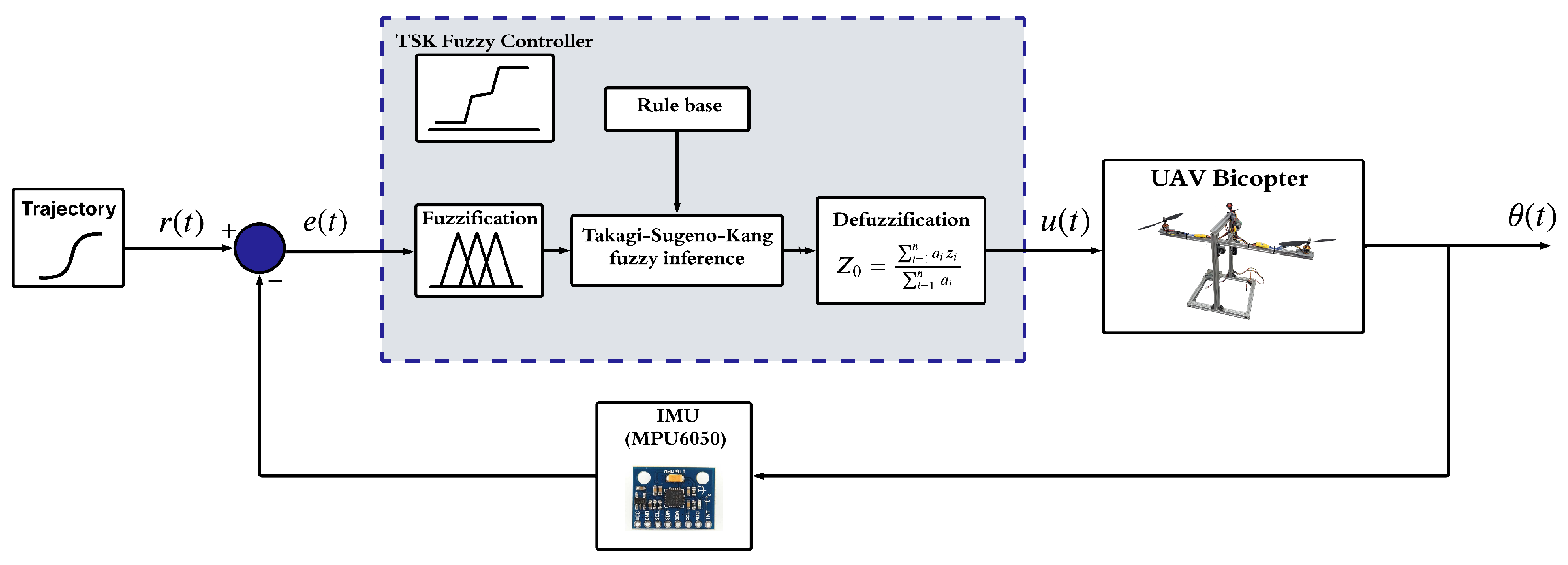
The structure of the TSK fuzzy controller consists of four stages: fuzzification, rule formulation, TS fuzzy inference, and defuzzification.
Fuzzification: This stage assigns each input a degree of membership to the defined fuzzy sets, enabling a qualitative representation of the system’s quantitative information. Each input variable is transformed into linguistic variables through fuzzy membership functions.
Rules formulation: The designer specifies the decision-making rules based on the relationship between the inputs and outputs.
TS fuzzy inference: In this stage, the TS fuzzy inference links the rules established in the previous stage with the outputs. This fuzzy inference relates the rules to the linear output functions proposed by the designer.
Defuzzification: Finally, in the defuzzification stage, a crisp output is obtained from the linear output functions using a weighted average, as seen in Equation (
11).
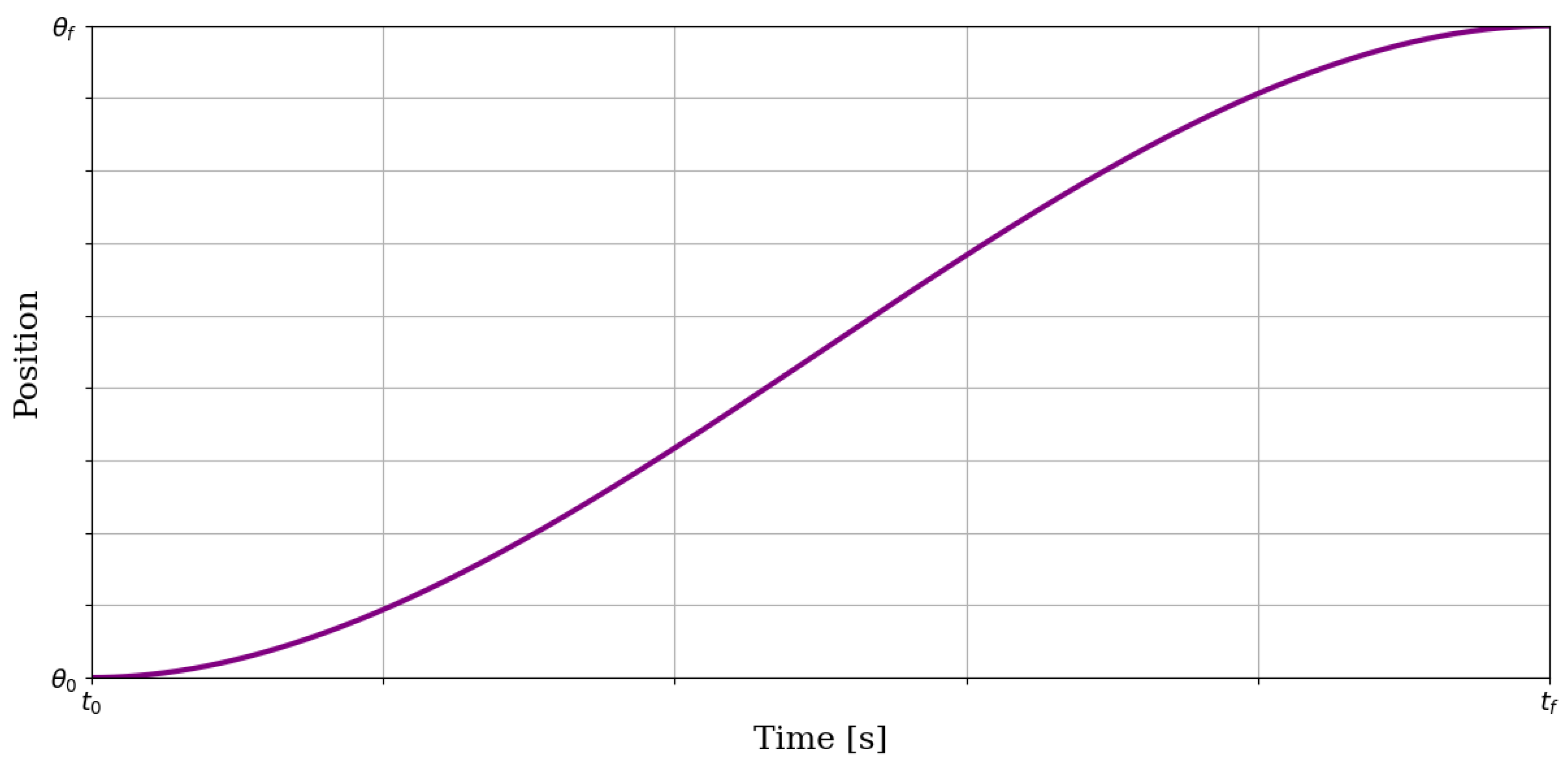
2.5. Parabolic Trajectory
In control systems, a trajectory refers to the path a system follows through a sequence of movements within a specified time frame. One of the most widely used methods for generating such trajectories is the parabolic velocity profile [
34], which provides smooth and predictable motion. This model accelerates the actuator at a constant rate until a midpoint is reached, followed by a symmetrical deceleration phase until the velocity returns to zero.
Equation (
12) defines the resulting position over time, which describes the displacement at each instant.
Figure 3 and
Figure 4 illustrate this parabolic trajectory’s corresponding position and velocity profiles.
Equation (
13) relates the velocity and the execution time of the motion.
3. Materials and Methods
The Takagi–Sugeno–Kang controller is the fuzzy controller presented in this research. This methodology is a rule-based control approach that combines fuzzy logic with linear models to handle complex, nonlinear systems.
Figure 5 illustrates the methodology employed in the design of the TSK fuzzy controller. The first step is to generate the parabolic trajectory presented in
Section 2.5, where the designer specifies the target final position and the execution time of the motion. The next step is the fuzzification process, in which linguistic variables are proposed based on the angular error exhibited by the system through membership functions. The third step is establishing the IF–THEN rules that relate the inputs to the outputs. Subsequently, the rules are evaluated through TS fuzzy inference. The next step is to perform defuzzification using Equation (
11) in
Section 2.3, where the output of the controller is computed as a weighted average of the rule outputs, with the weights determined by the firing strengths of the rules. The final stage corresponds to sending the control signal to both rotors of the UAV bicopter, denoted by
, to correct the error presented by the system.
The error denoted by
is defined as the difference between the reference or target position
and the current position measured by the angular sensor denoted by
, as shown in Equation (
14).
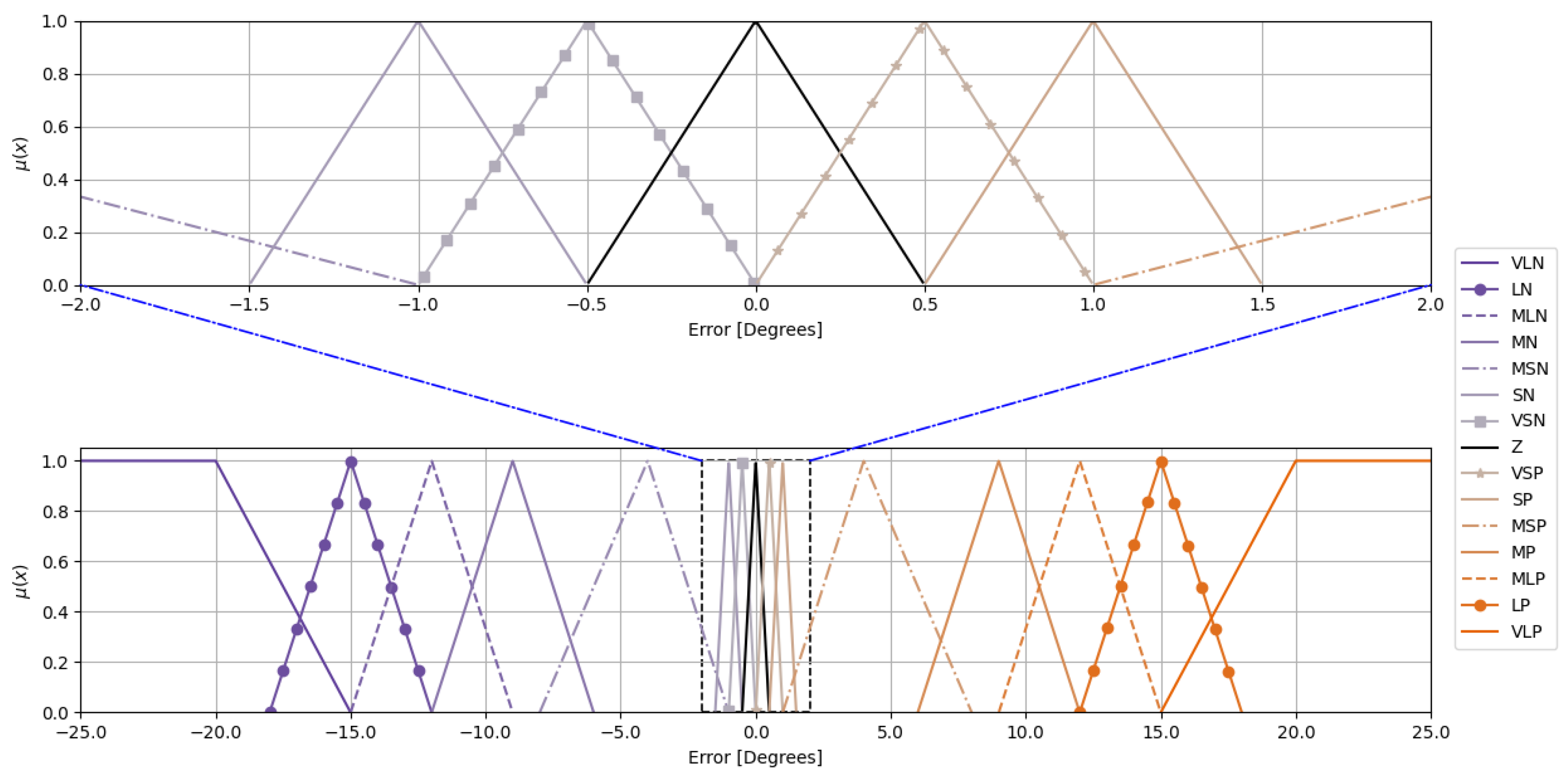
The fuzzification stage is based on the angular error using fifteen linguistic values. The linguistic values that describe it are shown with the following abbreviations: VLN (Very Large Negative), LN (Large Negative), MLN (Moderately Large Negative), MN (Medium Negative), MSN (Moderately Small Negative), VSN (Very Small Negative), Z (Zero), VSP (Very Small Positive), SP (Small Positive), MSP (Moderately Small Positive), MP (Medium Positive), MLP (Moderately Large Positive), LP (Large Positive), and VLP (Very Large Positive).
The linguistic variable (error) is described by two trapezoidal and thirteen triangular linguistic values. Equations (
15) and (
16) present the triangular and trapezoidal membership functions, respectively.
For the triangular membership function, , , and represent the start, the central point, and the end, respectively. For the trapezoidal membership function, , , , and represent the start, the left central point, the right central point, and the end, respectively.
The distribution of the linguistic values is symmetrically arranged to ensure a similar system response when the error takes on either positive or negative values. Trapezoidal membership functions are proposed to provide a constant response when the error becomes significantly large. On the other hand, triangular membership functions are employed at the center of the distribution because the system requires a fast and precise response to correct the error due to nonlinearities.
Figure 6 illustrates the symmetrical distribution of the linguistic values used to represent the error.
Table 3 presents the linear output functions associated with the proposed TSK fuzzy tracking controller. The table is divided into two sections representing the output control functions
and
, which are applied to the two rotors (BLDC1 and BLDC2 motors) of the UAV bicopter. For each linguistic rule
, a specific linear function of the form
is designed to adjust the controller response. The outputs for
start with positive coefficients
and progressively symmetrically shift toward negative values. In contrast,
starts with negative coefficients and gradually shifts to positive values. This symmetric distribution ensures a balanced and coordinated actuation of both rotors. However, this symmetry only holds if the motors have the same characteristics. In practical applications, where slight differences between motors may exist, the symmetry can be complemented, allowing the use of a reduced set of 15 IF–THEN rules while maintaining effective control.
Table 4 shows the fuzzy inference rules defined for the proposed TSK fuzzy tracking controller. Each rule follows the IF–THEN structure. Thirty fuzzy rules are proposed, with fifteen fuzzy rules for each output (
,
).
The defuzzification stage is evaluated based on a weighted average, as shown in Equation (
11). Therefore, Equations (
17) and (
18) determine the output values for both rotors.
To quantify the performance tracking controller, it is evaluated using the Root Mean Squared Error (
RMSE) and the Integral Absolute Error (
IAE). Equation (
19) defines the calculation of the RMSE, which evaluates the average error between the system’s behavior and the target position. On the other hand, the IAE computes the total accumulated error during the entire test duration. Its expression is defined in Equation (
20).
where
N is the total number of samples.
is the position value at sample k.
is the target position value at sample k.
is the sampling time.
4. Results
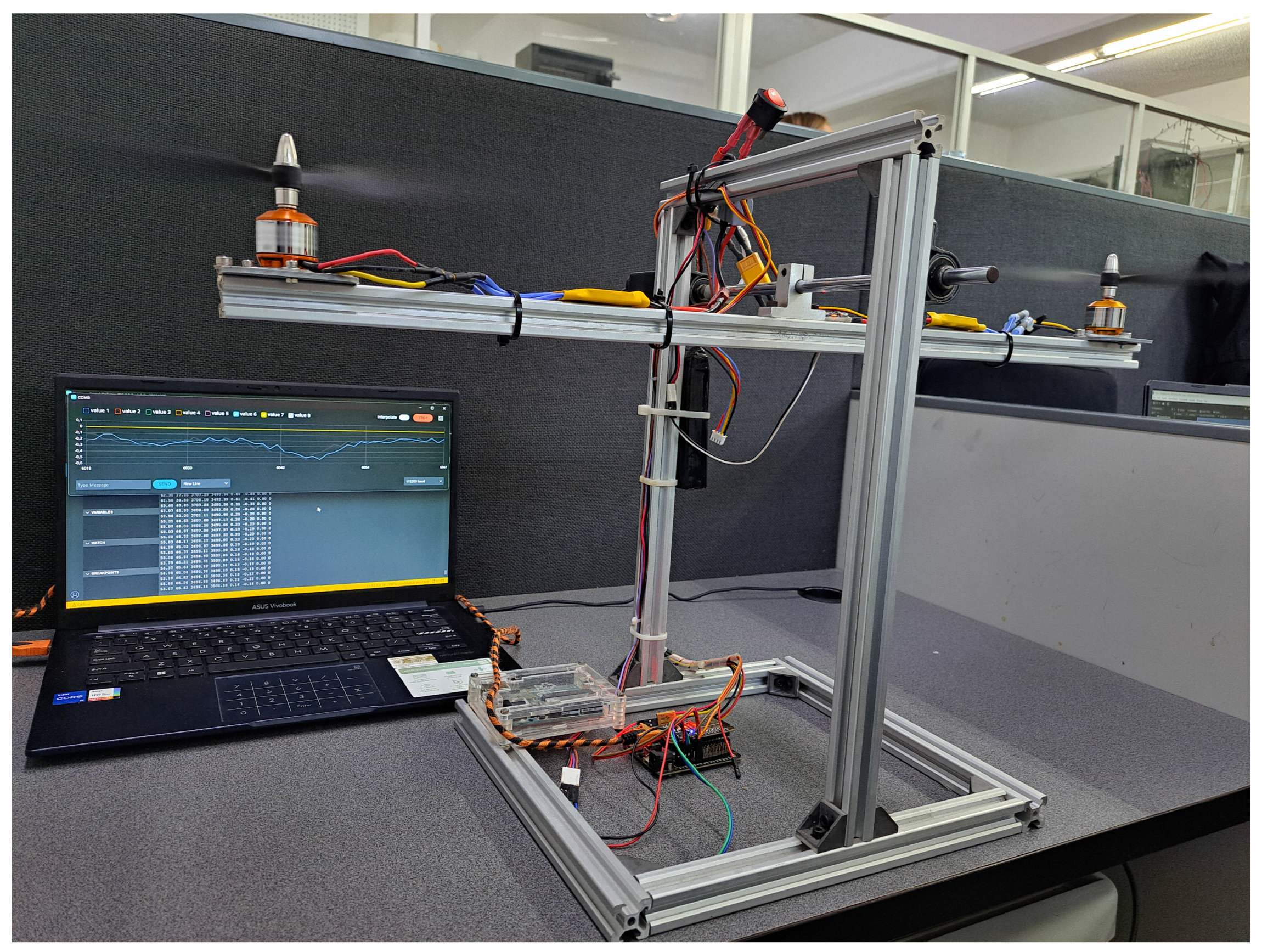
This section presents the final design of the TSK fuzzy tracking controller. The fuzzy tracking controller is implemented on an embedded system based on the ESP32 microcontroller. The MPU6050 sensor is responsible for acquiring the angular position data measured from the UAV bicopter. The embedded system is programmed in C++ using a sampling time of 0.02 s for the experimental phase. The execution time of the implemented TSK fuzzy controller has an average execution time of 387.8063 μs per control cycle. This execution time includes evaluating membership functions, the fuzzy inference process, and calculating the controller output. The selected sampling time is constrained by the physical limitations of the BLDC motors, which cannot adjust their rotational speed instantaneously due to the rotor’s mechanical inertia. As a result, several milliseconds are required for the motor to respond effectively to changes in the PWM signal.
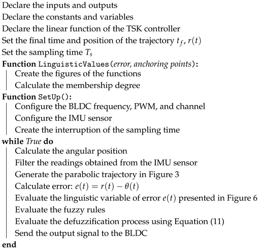
Figure 7 illustrates the mechanical system of the UAV bicopter in experimentation. Algorithm 1 shows how the TSK fuzzy tracking controller works.
| Algorithm 1: TSK fuzzy tracking controller algorithm. |
![Symmetry 17 00759 i001]() |
Table 5 shows the distribution parameters of the triangular and trapezoidal error linguistic values.
Figure 8 illustrates the visual representation of the membership functions used in the final controller proposal. The distribution of the functions closer to zero aims to achieve a fast system response within the error range of [−1.5 to 1.5] degrees, reducing the steady-state error.
Table 6 presents the linear functions used in the final test. These functions are based on the response required by the system to overcome the inherent nonlinearities of the UAV bicopter. A quicker response is needed to stabilize the system when the error ranges from 0.5 to 1.5 degrees. Due to the nonlinearity, the UAV bicopter can enter steady-state error if a smoother response is observed within this range of values. The definition of the coefficients
and the constant terms
in the output linear functions of the TSK fuzzy controller follows a design process to ensure robust and precise system performance in response to variations in the reference error. The main objective in selecting these coefficients is to reduce the steady-state error, considering the system’s inherent nonlinearities. Rapid and aggressive corrections are applied to achieve this in scenarios where immediate stabilization of the target position is required. In contrast, smoother corrections are used in situations far from the reference position to avoid oscillatory movements that could compromise the system’s stability.
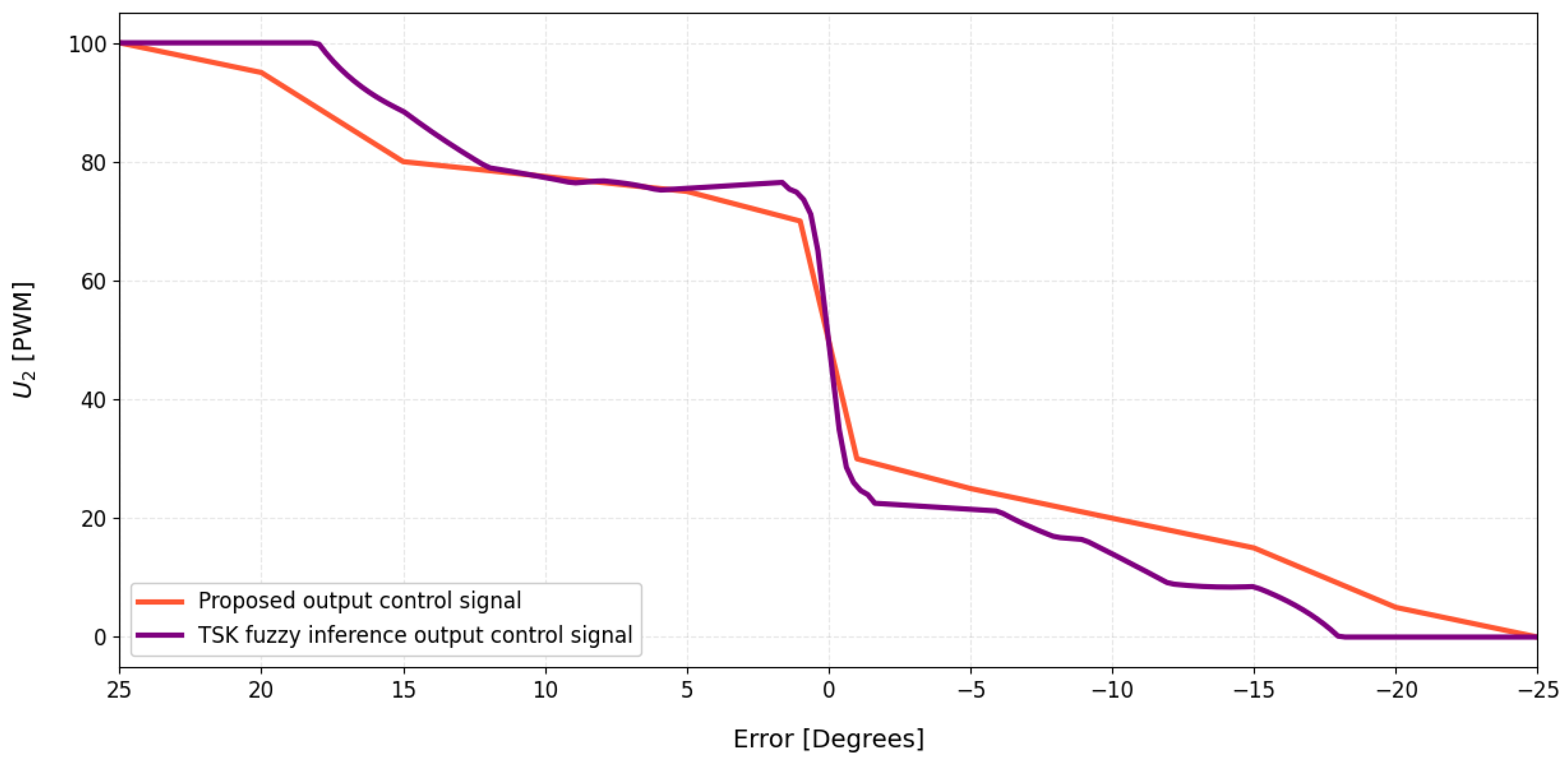
Figure 9 and
Figure 10 show the control output surfaces obtained through the TSK fuzzy inference and the expected designed control surface. Although the expected control surface was designed using linear segments, the control signal processed through the TSK fuzzy inference system exhibits nonlinear behavior. This distortion arises from the nature of the membership functions employed, which influence the weighted combination of the local outputs. With two trapezoidal membership functions at the extremes, a slower response is obtained to prevent the system from aggressively correcting the error. In contrast, implementing the triangular functions for small angular errors generates a faster response to correct the system’s output. The asymmetry in the output surface between the two rotors arises because the rotors do not have identical mechanical characteristics, causing them to break inertia in different ways. As a result, 15 fuzzy rules are proposed for each motor to account for their differing behaviors.
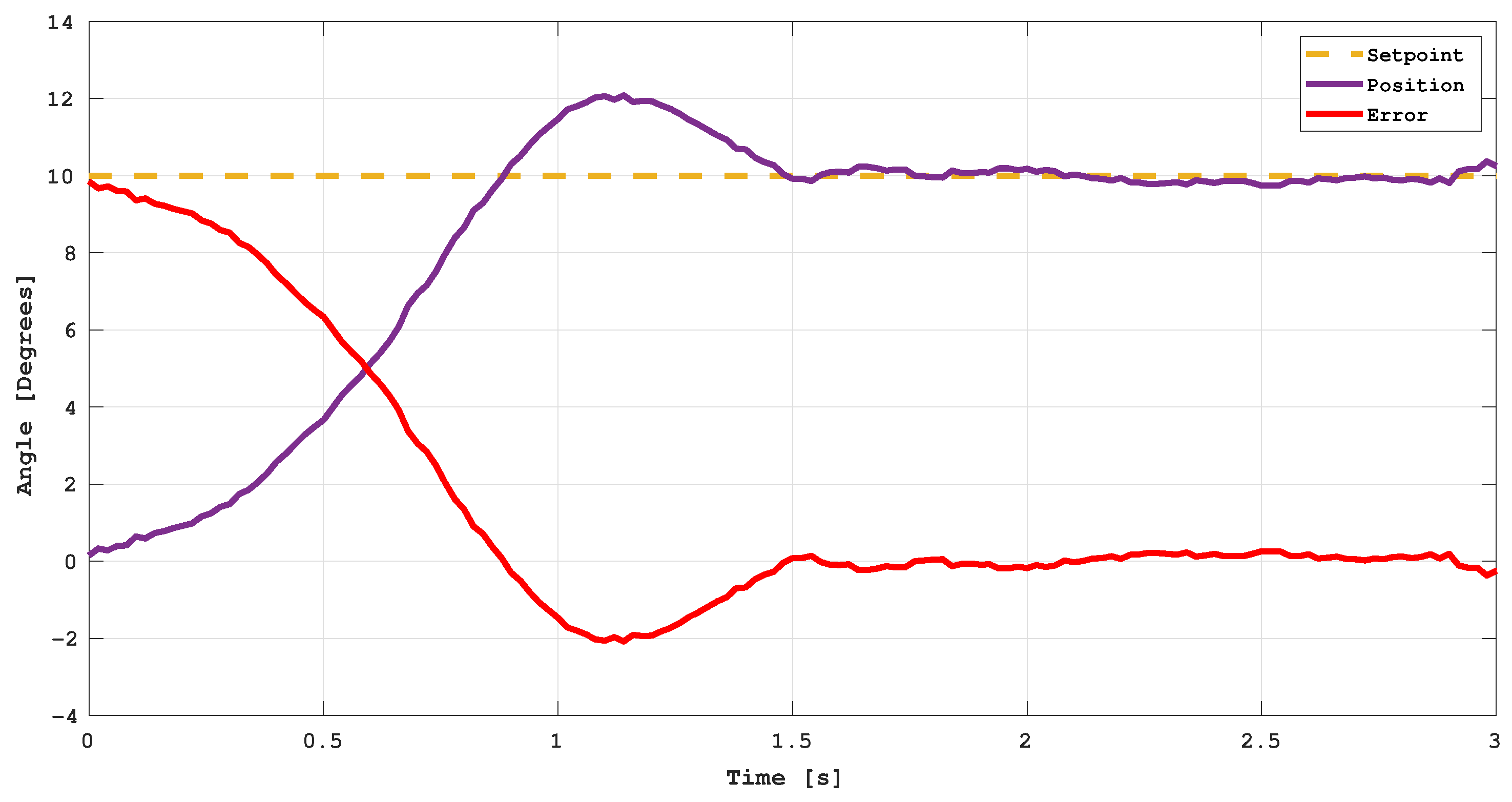
The first test was conducted to evaluate the performance of the TSK controller using a target position corresponding to a 10-degree step input, as illustrated in
Figure 11. The system is stabilized within 1.5 s, achieving a minimal steady-state error of 0.25 degrees.
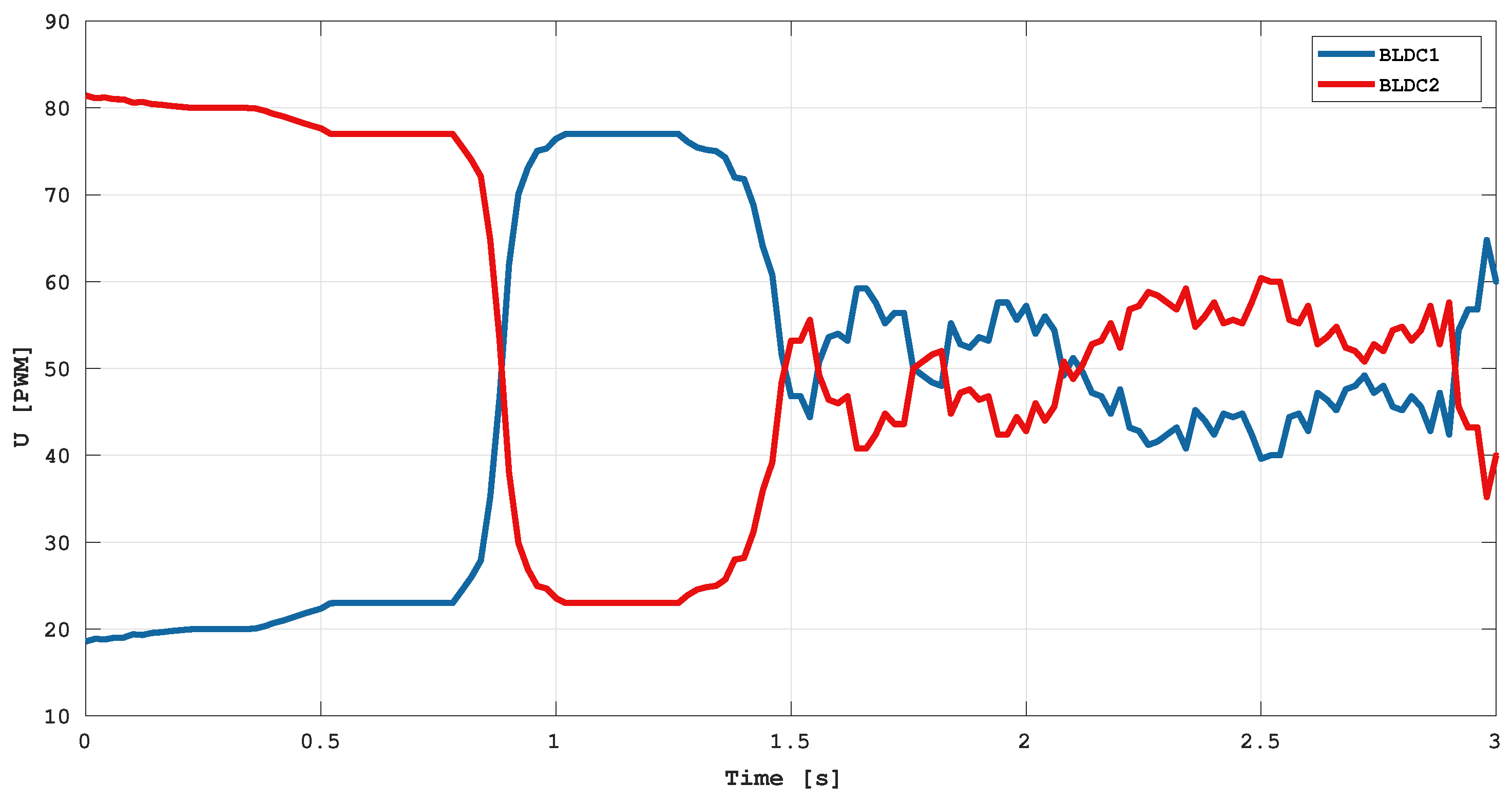
Figure 12 presents the control signal applied in the step-test.
The experimental results are presented in five different trajectory tracking cases, with the main objective being to validate that the TSK controller successfully stabilizes the proposed system within the target time. For the five cases, a final time of 1.7 s is proposed.
Figure 13 illustrates the angular position response of the system under the control of the TSK fuzzy controller. The reference trajectory is compared with the actual angular position obtained during the experiment.
Figure 14 shows the angular error reported during several tests.
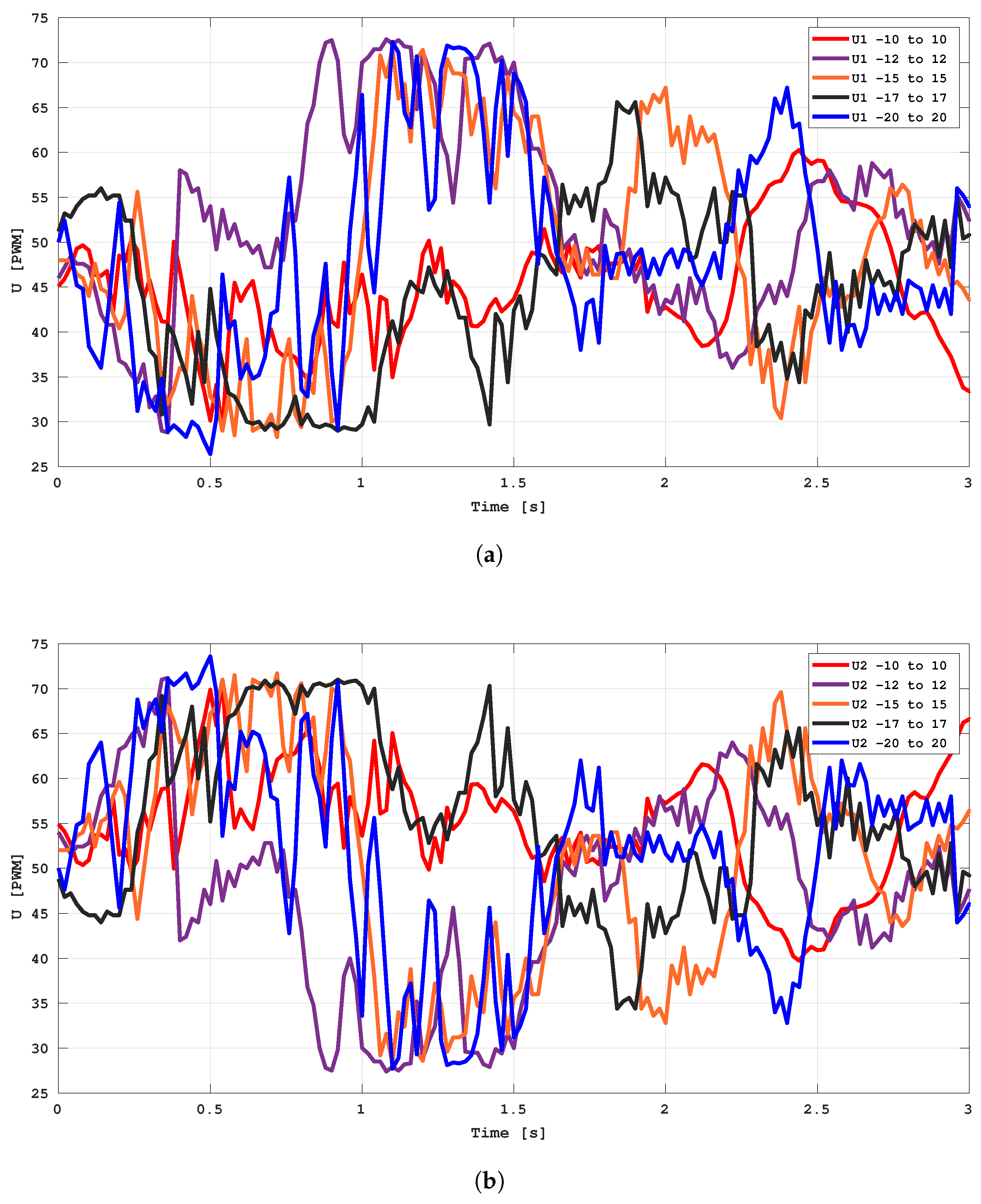
Figure 15a,b show the control signals
and
, respectively, applied to the rotors during each trajectory tracking test. These signals reflect the controller’s dynamic response to the desired reference inputs. The variation in the PWM levels for each rotor illustrates how the system adjusts the actuation to maintain stability and accurately follow the desired trajectory.
On the other hand, the first test starts at an initial position of −10 degrees and ends at the final position of 10 degrees. The maximum angular error observed during the experiment test is 0.6 degrees, while the steady-state error is 0.415. The system exhibits an RMSE value of 0.2049 and an IAE value of 0.9876. Additionally, the OS recorded during the test was 2.89915%. The second test from −12 to 12 reports an RMSE value of 0.3269 and an IAE of 2.7460, with a steady-state error of 0.35 degrees and an overshoot (OS) of 1.8333%, making it the trajectory case with the lowest values obtained. The third test starts from an initial position of −15 and ends at the final position of 15 degrees. The bicopter shows a steady-state error of 0.49 degrees, while the OS obtained during the test was 2.866%. This test presents an RMSE value of 0.3899 and IAE value of 2.5244. The four tests from −17 to 17 present an IAE value of 2.27615 and an RMSE value of 0.3335. The system shows a steady-state error of 0.39 degrees, while the overshoot obtained during the test was 2.294%. The fifth test begins at −20 degrees and reaches a final position of 20 degrees. The maximum angular error recorded was 0.86 degrees, while the steady-state error measured 0.43 throughout the experimental test. The system achieved an RMSE of 0.2494 and an IAE of 1.1799. Furthermore, the overshoot observed during the test was 1.1799%.
Robustness Test
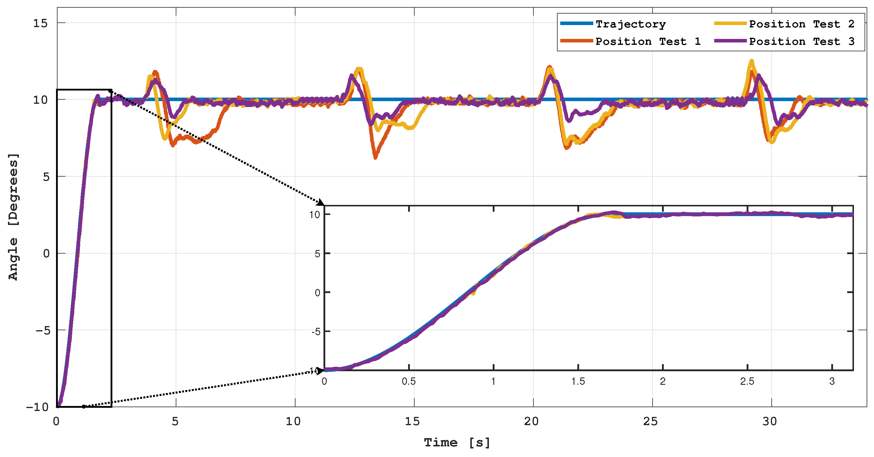
Figure 16 presents three scenarios of robustness tests applied to trajectory tracking within an angular range of −10 to 10 degrees. These tests aim to evaluate the capability of the proposed controller to maintain system performance under external disturbances. The methodology used to induce such disturbances involves periodically altering the target position. Every 8 s, the cycle duty of one rotor is increased to 90% while the other is decreased to 10% for a brief interval of 500 milliseconds. This abrupt and cyclical modification of the rotors’ duty cycle is designed to temporarily destabilize the system, enabling the analysis of the controller’s response to unexpected variations in the desired trajectory. The results of each test allow for the assessment of the controller’s effectiveness in terms of recovery, stability, and accuracy under unanticipated external conditions. The system initially tracks the generated parabolic trajectory. Once the steady-state error is reached, the computationally generated perturbations are introduced. The response demonstrates the effectiveness of the controller under perturbations, as it returns to the target position after the disturbance.
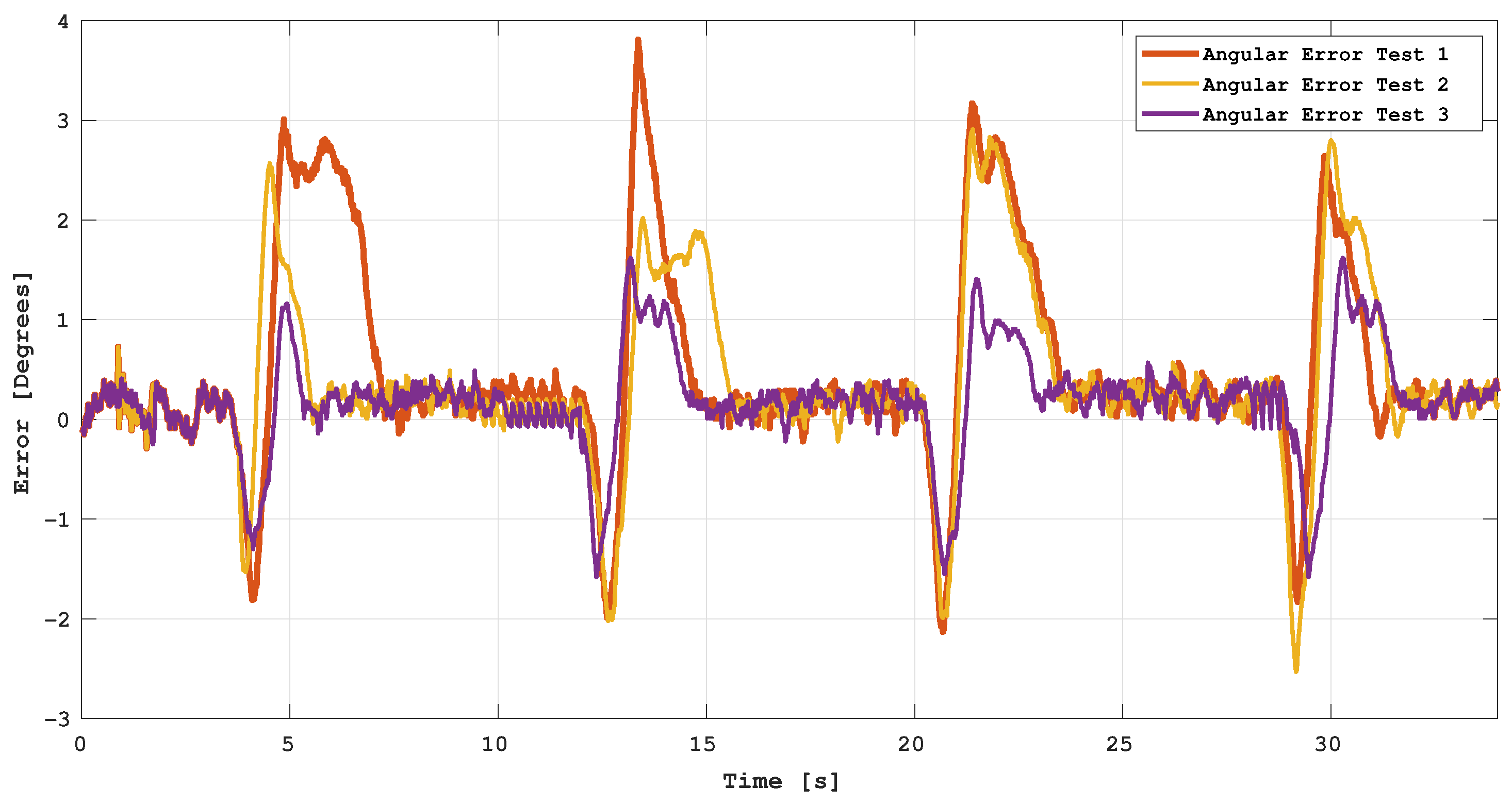
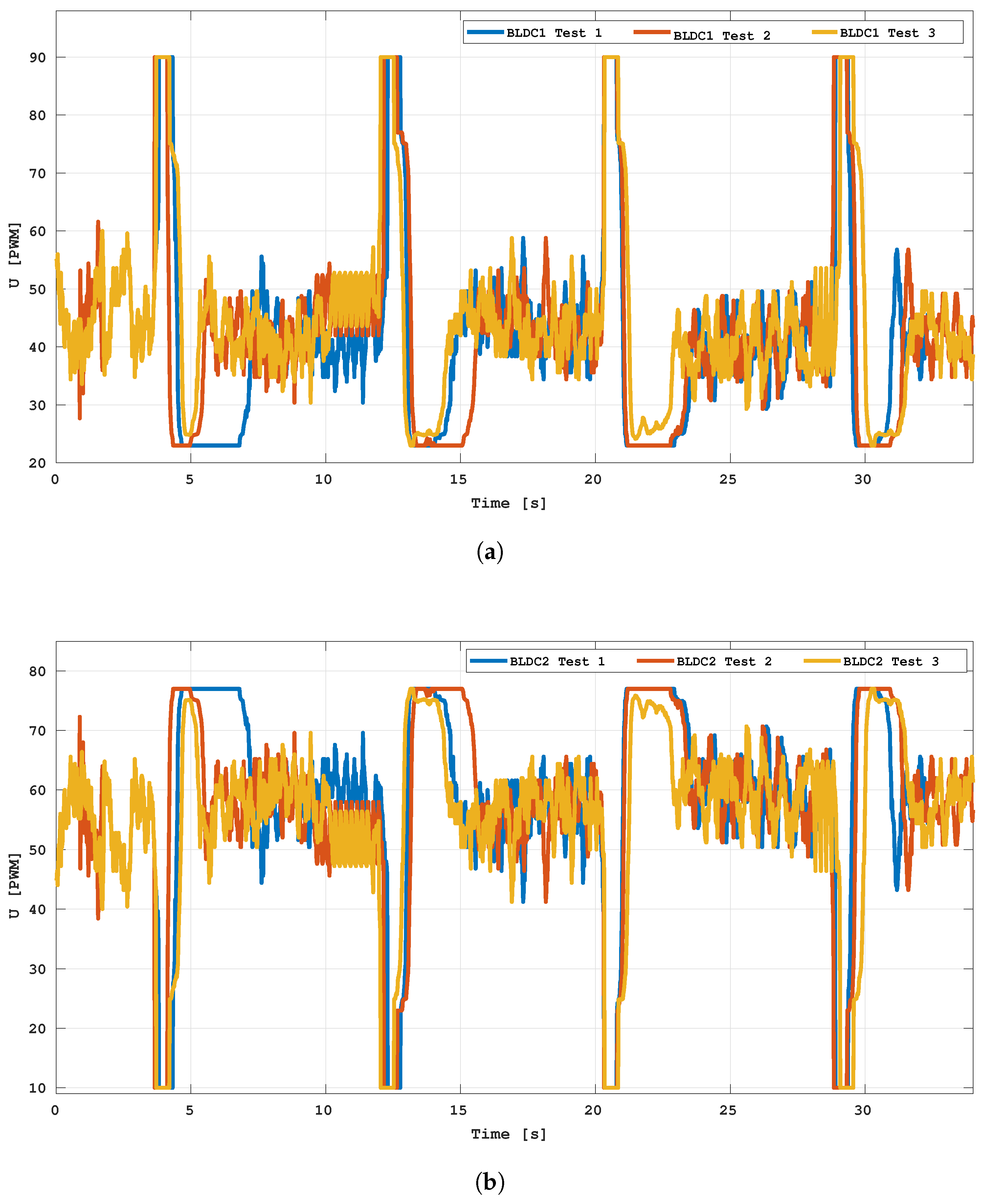
Figure 17 shows the error observed during the tests. On the other hand,
Figure 18a,b present the control signals
and
, respectively, applied to rotors in three tests.
5. Discussion
Figure 13 presents several trajectory tracking tests on the proposed control system. In all cases, the settling time was consistently 1.7 s. The first test yielded the lowest root mean square error (RMSE) of 0.2049 and the lowest integral of absolute error (IAE) of 0.9876, while the second test exhibited the smallest overshoot at 1.8333%. The fourth test achieved the lowest steady-state error, with a final deviation of only 0.39 degrees. Complementarily,
Figure 14 compares the angular errors across all experiments: the fifth test recorded the highest angular error (0.86 degrees), whereas the fourth test again stood out with the lowest error (0.6 degrees). To validate the trajectory tracking strategy’s robustness, 100 experimental trials were performed—50 within the range of
to 10 degrees and 50 within
to 20 degrees. The TSK fuzzy controller demonstrated consistent performance, achieving low average RMSE values and small standard deviations in both scenarios, reflecting high accuracy and stable system behavior. Although the IAE increased slightly in the broader range, it remained within acceptable margins, confirming the controller’s capacity to manage larger reference deviations without significant cumulative error. The average duration of the trajectory tracking trials was approximately 9 s, as summarized in
Table 7.
For the 10-degree step input test, the overall mean error was 0.2268 with a standard deviation of 0.055, while the mean of individual standard deviations was 0.1428 (±0.0316), reflecting a consistent and precise system response. These results were obtained from 50 experimental trials, each with an average duration of 14 s, demonstrating the thoroughness of our experimental process.
Table 8 presents a comparative analysis with other related methodologies implemented on similar UAV configurations. Four case studies are considered: the first employs an AF2-DOF PID controller for a two-rotor UAV, providing only simulation results; the second focuses on balancing control through optimization of the Q and R parameters in a bicopter, also limited to simulations; the third implements a classical PID controller for experimental bicopter control; and the fourth explores pitch regulation using a state feedback controller, again through simulation. Compared to these approaches, the proposed TSK fuzzy controller offers experimentally validated results and superior tracking precision under real-world conditions.
Table 9 presents a comparative analysis of key performance metrics—RMSE, IAE, steady-state error (SE), overshoot (OS), and settling time (ST)—between the proposed methodology and several related works. In the study by [
19], the controller achieved an SE of 0.05 and an ST of 0.0867 s, with no overshoot reported. While these results indicate a highly efficient response, they are limited to simulation-based validation. Similarly, ref. [
17] applied a genetic algorithm for parameter optimization and obtained an OS of 12.8244% and an ST of 7.1450 s, also without steady-state error; however, this approach was likewise validated only through simulation. In contrast, ref. [
16] reported experimental results on a bicopter, achieving an SE of 0.25 degrees, an OS of 6.68%, and a settling time of 2.62 s. Another simulation-based study by [
35] employed a state feedback controller for pitch regulation, showing an OS of 4.86% and an ST of 1.13 s, with no steady-state error. The methodology proposed in this article differs by incorporating both simulated and experimentally validated results, reporting RMSE and IAE values of 0.2049 and 0.9876, respectively—performance indices not addressed in the studies above. Additionally, it achieved an SE of 0.415 degrees and an OS of 2.8915%, with a target settling time of 1.7 s. Although the proposed method exhibits a higher steady-state error than that reported in [
16], it ranks third in settling time among all compared approaches. These results not only reflect the challenges imposed by the system’s inherent nonlinearities and experimental uncertainties but also demonstrate a competitive and practically viable control performance, providing reassurance and confidence in its application.
6. Conclusions
This paper introduced the design and experimental implementation of a TSK fuzzy controller for trajectory tracking in a UAV bicopter, characterized by strong nonlinearities and dynamic complexity. The proposed strategy demonstrated high tracking accuracy, achieving low RMSE and minimal steady-state deviations across all test scenarios. Quantitative metrics such as RMSE and the integral of absolute error (IAE) validated the controller’s precision and robustness. All experiments yielded consistent settling times of approximately 1.7 s. The most favorable trajectory exhibited an RMSE of 0.2049 and an IAE of 0.9876. Furthermore, the controller maintained effective performance under external computational disturbances. When a sudden perturbation was introduced to one of the rotors, the system quickly stabilized and returned to the desired trajectory, with a maximum angular deviation of only 3.81 degrees. These results highlight the controller’s strong disturbance rejection capabilities and ability to ensure stable operation in real-world conditions. The practical implementation confirmed the viability of the proposed TSK fuzzy approach, reinforcing its relevance for applications requiring real-time, reliable control in uncertain and nonlinear environments. In summary, the results underscore the effectiveness of the TSK controller as a robust solution for precise trajectory tracking in UAV systems. Beyond the current scope, this case study opens several avenues for future research. One direction involves developing an adaptive version of the controller that can modify its fuzzy rules in real-time based on changing system dynamics. Another promising extension is the integration of neuro-fuzzy architectures, enabling learning from simulations and experimental data. Perhaps the most ambitious line of inquiry is scaling the approach to multicopter platforms—tricopters, quadcopters, or hexacopters—thus enabling three-dimensional trajectory tracking through coordinated control of altitude, pitch, and roll.


 ,
, 


