An Enhanced Fuzzy Time Series Forecasting Model Integrating Fuzzy C-Means Clustering, the Principle of Justifiable Granularity, and Particle Swarm Optimization

Abstract

In this paper, we propose a novel fuzzy time series forecasting model that integrates fuzzy C-means (FCM) clustering, the principle of justifiable granularity (PJG), and particle swarm optimization (PSO), with a focus on leveraging symmetry in subinterval partitioning to enhance model interpretability and forecasting accuracy. First, the FCM method is employed to partition the universe of discourse, generating an initial division of subintervals. To ensure symmetric information representation, triangular fuzzy information granules are constructed for these subintervals in accordance with the principle of justifiable granularity. Then, an objective function is formulated for the entire universe of discourse, and the PSO algorithm is utilized to optimize the subinterval division, resulting in the final optimal partition. This process ensures that the subintervals achieve a balance between coverage and specificity, thereby introducing a form of symmetry in the partitioning of the universe of discourse. Leveraging the optimized symmetric partition, the framework of the fuzzy time series model is implemented for forecasting. Finally, the proposed approach is carried out on the Taiwan Weighted Stock Index (TAIEX) datasets and the Shanghai Composite Index (SHCI) datasets. The forecasting results demonstrate that the proposed approach achieves higher prediction accuracy and semantic accuracy compared with other methods.

1. Introduction

A time series is a sequence of observations recorded in chronological order, which essentially reflects the trend of one or more random variables changing over time. The primary goal in time series forecasting lies in extracting the inherent patterns from historical data and then utilizing these patterns for future value prediction. In real life, time series can be extensively applied across numerous domains, including stock index forecasting [1], hydrometeorology forecasting [2], enrollment forecasting [3], temperature forecasting [4], etc.

Conventional time series forecasting techniques mainly encompass several statistical models, including the Auto Regressive (AR) model, the Auto Regressive Moving Average (ARMA) model, and the Auto Regressive Integrated Moving Average (ARIMA) model [5]. These approaches center on estimating the parameters of the fitted models, which are then applied for forecasting purposes. Nevertheless, their restrictive assumptions and parametric characteristics restrict their effectiveness. As machine learning continues to advance, methods like Support Vector Machines (SVM) [6,7], Convolutional Neural Network (CNN) [8,9], and Long Short-Term Memory (LSTM) recurrent neural network [10,11] have also demonstrated remarkable effectiveness in time series forecasting. Despite their ability to address most real-world problems, these methods still face unresolved challenges involving fuzzy and uncertain data. Over the past few years, a growing trend has emerged in developing time series forecasting methods grounded in fuzzy set theory to tackle these issues.

In 1965, Zadeh [12] established fuzzy theory to address problems involving uncertain and fuzzy linguistic variables. In 1985, Sugeno and Tanaka [13] began to use fuzzy models to model and predict complex systems. Based on Zadeh’s fuzzy set theory, Song and Chissom [14,15] developed a prediction model for fuzzy time series in 1993, which expounded the framework involving fuzzy relation equations and approximate reasoning processes, thereby initiating the theoretical and practical research in this area. A traditional time series forecasting model comprises these four steps: (1) partitioning the universe of discourse, (2) defining fuzzy sets and fuzzifying the historical time series, (3) establishing fuzzy logical relationships of the fuzzy time series, and (4) forecasting and defuzzifying the fuzzy time series. Among these steps, step (1) serves as the cornerstone for fuzzy time series modeling [16] and represents the current focal point in fuzzy time series forecasting.

In 1993, Song and Chissom [17] were the first to propose the equal-interval partition technique for the universe of discourse, applying it to forecasting in fuzzy time series. Huarng [18,19] conducted extensive studies on how interval length affects forecasting outcomes. They proposed interval partitioning methods based on distribution, average value, and growth ratio, all of which proved to be superior in highlighting data structure and improving forecasting accuracy. Chen [20] carried out interval division according to the density of the sample data distribution following the principle of fine division in dense areas and coarse division in sparse areas. Chen et al. [21] first divided the universe of discourse using an equal-frequency method and then employed an entropy-based discretization iterative technique to granulate the fuzzy time series‘ universe of discourse. Wang et al. [22,23] combined the concept of information granulation in granular computing with fuzzy C-means clustering and Gath–Geva clustering to partition the universe of discourse in fuzzy time series, which improved the model’s accuracy. Yin et al. [24] proposed the interval type-2 FCM algorithm to replace the traditional FCM for dividing the sample domain, thereby enhancing the effectiveness of the FTS model. Recently, the principle of justifiable granularity (PJG) has been utilized in designing interval type-1 and type-2 fuzzy sets [25,26,27,28]. Furthermore, some scholars [29,30,31] have incorporated optimization algorithms to determine the optimal partitioning of subintervals within the universe of discourse. The optimal partitioning values for the intervals within the universe of discourse are frequently identified using the particle swarm optimization (PSO) algorithm [32,33,34,35]. Xian et al. [36] applied a hybrid artificial fish swarm optimization algorithm to determine the lengths of the intervals.

In sum, the above methods are summarized into four types. (1) Partitioning the universe of discourse with equal interval: This approach is easy to implement but lacks interpretability, failing to effectively reflect the distribution characteristics of datasets with uneven data distribution. (2) Partitioning the universe of discourse with equal frequency: This approach can intuitively show the data distribution and make it easy to understand the central tendency of data. However, it is insensitive to extreme values and limited to handling complex distribution data. (3) Partitioning the universe of discourse based on the clustering method: This method can effectively identify the internal structures and patterns within the data. However, it is vulnerable to the influence of outliers, and the number of data points within the intervals is unbalanced. (4) Partitioning the universe of discourse based on an optimization algorithm: This method usually depends on the setting of the objective function. Generally, these methods cannot simultaneously meet the requirements of both the interpretability of the intervals for dividing the universe of discourse and the prediction accuracy. Therefore, it is necessary to design a method for information granulation of the time series’ universe of discourse that can not only have strong interpretability but also achieve high prediction accuracy.

In this study, a new fuzzy time series forecasting model is proposed that integrates fuzzy C-means clustering, the principle of justifiable granularity, and particle swarm optimization. Firstly, we use the FCM method to divide the universe of discourse to obtain the initial subintervals division. Next, fuzzy information granules are constructed for the subintervals based on the principle of justifiable granularity. Then, an objective function is set for the entire universe of discourse, and the PSO algorithm is applied to obtain the final result of the optimal subintervals division. Based on the optimal partition results, we perform the framework of the fuzzy time series model for forecasting. Finally, we apply this approach to the TAIEX and SHCI datasets, comparing the forecasting results with other methods to demonstrate the effectiveness of the proposed forecasting model.

The remainder of this article is organized as follows. In Section 2, we review some relevant prerequisites. Section 3 presents a novel approach to segmenting the universe of discourse for time series data, utilizing fuzzy C-means clustering and information granulation. Section 4 details the specific steps of the fuzzy time series forecasting model, leveraging the optimal partition of the universe of discourse. Section 5 carries out some experiments to demonstrate the performance of the proposed forecasting model. Section 6 concludes this study.

2. Preliminaries

In this section, we offer a succinct review of the fundamental theories, including the fuzzy time series model, the fuzzy C-means clustering, triangular fuzzy information granules, the principle of justifiable granularity, and the particle swarm optimization algorithm.

2.1. Fuzzy Time Series Model

A fuzzy time series is a descriptive form of time series based on fuzzy theory, which simulates human cognition of the natural world. Each data object in the fuzzy time series is a semantic value. By constructing fuzzy logical relationships among these semantic values, the dynamic evolution process of the time series can be described, and its fuzzy change rules can be obtained. Traditional time series are usually recorded with precise values. However, in real life, the changes of many things often cannot be represented by precise numerical values. Moreover, the method of representing with precise numerical values does not conform to the cognitive patterns of human beings. Humans tend to understand and express things in a language form that they can understand. For example, when people perceive the temperature in a certain area, they usually describe the temperature level with words like “extremely cold”, “very cold”, “cold”, “hot”, “very hot”, “extremely hot”, etc., rather than specific temperature values. On the one hand, specific temperature data need to be measured with devices such as thermometers, and in the absence of measuring devices, the current information cannot be recorded in a timely manner. On the other hand, everyone has a different perception of temperature, and usually has their own judgment criteria. Recording the semantic values of temperature in chronological order results in a time series composed of fuzzy semantic values.

Song and Chissom [14] initially introduced the concept of fuzzy time series. The fundamental definition is provided as follows.

Definition 1.

Fuzzy Set (FS).

Let U denote the universe of discourse and $U=\{u_1,u_2,\dots ,u_n\}$ be an order segmentation set. Define A as a fuzzy set on U, which is expressed as:

$$A={\displaystyle \frac{f_A(u_1)}{u_1}}+{\displaystyle \frac{f_A(u_2)}{u_2}}+\dots +{\displaystyle \frac{f_A(u_n)}{u_n}}$$

(1)

where f_A denotes the fuzzy membership function of the fuzzy set A; u_i is an element of the fuzzy set A_i; and f_A(u_i) indicates the degree to which u_i belongs to A_i, where $0\le f_A(u_i)\le 1$ and 0 ≤ i ≤ n.

Definition 2.

Fuzzy Time Series (FTS).

Let $Y(t)(t=\dots ,0,1,2,\dots )$ be a subset of U and $f_i(t)$ be a collection of fuzzy sets defined on Y(t). If $F(t)=\{f_1(t),f_2(t),\dots \}$ is an ordered set consisting of fuzzy sets $f_i(t)$, then F(t) is referred to as a fuzzy time series on Y(t).

Definition 3.

Fuzzy Relationship (FR).

Assume that R(t,t − 1) is the fuzzy relation from F(t − 1) to F(t), satisfying F(t) = F(t − 1)∘R(t,t − 1). In this case, F(t) is obtained from F(t − 1) via the fuzzy relation R(t,t − 1), which can be denoted as F(t − 1) → F(t). Here, “∘” represents the composition operation, F(t − 1) and F(t) are fuzzy sets, and R is the first-order fuzzy relation defined on F(t).

Definition 4.

Logical Relationship (LR).

Suppose F(t − 1) = A_i and F(t) = A_j; then, a fuzzy logic relation A_i → A_j can be employed to depict the consecutive observations F(t − 1) and F(t). Here, A_i is referred to as the left-hand part (antecedent), while A_j is termed the right-hand part (consequent) of the fuzzy relation.

2.2. Fuzzy C-Means Clustering

Fuzzy C-means (FCM) clustering, introduced by Bezdek et al. [37], is a clustering algorithm that incorporates fuzzy theory. Unlike traditional hard clustering algorithms like K-Means, the clustering results of FCM do not completely belong to or completely not belong to a certain cluster but are represented by membership degrees to indicate the extent of belonging to a certain class. The clustering results are more flexible and have found extensive application across diverse fields. The essence of the FCM clustering algorithm is to transform the clustering problem of a dataset into a constrained nonlinear programming problem. By optimizing and solving, the corresponding data partitioning and class prototypes are obtained. The algorithm is straightforward to implement and offers good semantic interpretation.

The optimization goal and constraints for FCM clustering are presented as follows:

$$J_{\mathrm{m}}(U,V)={\displaystyle \sum _{i=1}^N{\displaystyle \sum _{j=1}^C{u}_{\mathrm{ij}}^m{\Vert x_i-v_j\Vert }^2}}$$

(2)

$$s.t.\{\begin{array}{l}0\le u_{ij}\le 1,\forall i,j\\ {\displaystyle \sum _{j=1}^C{u}_{i\mathrm{j}}}=1,\forall j\\ 0\le {\displaystyle \sum _{i=1}^N{u}_{i\mathrm{j}}}\le N,\forall i\end{array}$$

(3)

where x_i denotes the data value, N is the total number of data points, C represents the number of clusters, m ∈ (1, +∞) is the fuzziness coefficient, u_ij indicates the membership degree of the i-th data point in the j-th cluster, V is the set of cluster centers, v_j describes the center of the j-th cluster, and ||∙|| represents the Euclidean norm.

Solving the objective function under the constraint conditions mainly consists of two steps: solving the membership degree u_ij and calculating the cluster center v_j. The FCM clustering algorithm employs an iterative method to minimize the objective function, with the corresponding formulas given as follows:

$$u_{ij}={\left[{\displaystyle \sum _{k=1}^C{\left(\frac{\Vert x_i-v_j\Vert }{\Vert x_i-v_k\Vert }\right)}^{\frac{2}{m-1}}}\right]}^{-1}$$

(4)

$$v_j={\displaystyle \frac{{\displaystyle \sum _{i=1}^N{u}_{ij}^m{x}_i}}{{\displaystyle \sum _{i=1}^N{u}_{ij}^m}}}$$

(5)

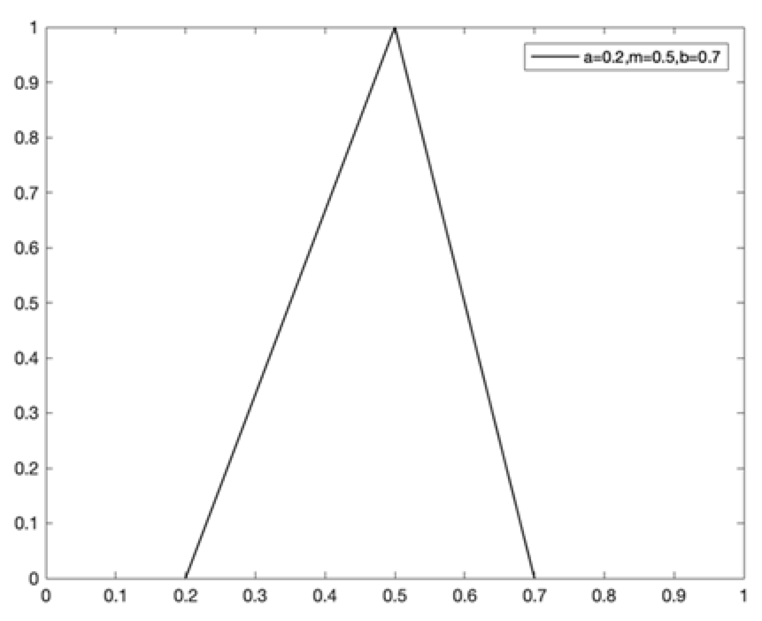
2.3. Triangular Fuzzy Information Granules

Fuzzy sets are usually used to represent information granules. Common methods for representing fuzzy information granules (FIGs) [38] include interval fuzzy information granules (IFIGs), triangular fuzzy information granules (TFIGs), gaussian fuzzy information granules (GFIGs), trapezoidal fuzzy information granules (TIGs), etc.

The membership function for a TFIG can be specified as follows:

$$A(x;a,m,b)=\{\begin{array}{l}0,x<a\\ {\displaystyle \frac{x-a}{m-a}},a\le x\le m\\ {\displaystyle \frac{b-x}{b-m}},m<x\le b\\ 0,x>b\end{array}$$

(6)

where x is a data point in the dataset X; a and b are the lower and upper supports of the triangular fuzzy set, respectively; and m is the core of the triangular fuzzy set. Figure 1 displays an example of a TFIG with a = 0.2, m = 0.5, b = 0.7.

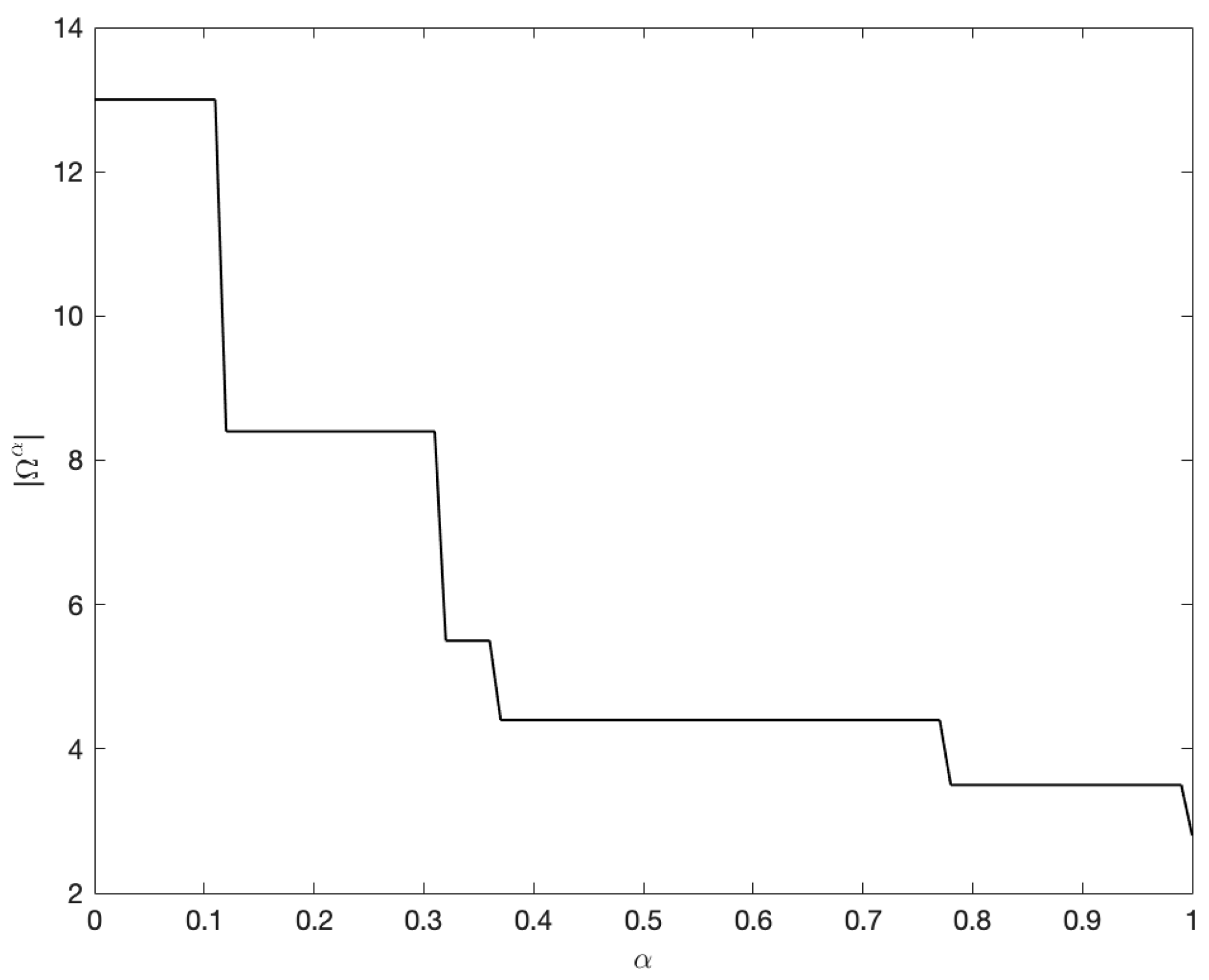
2.4. Principle of Justifiable Granularity

The principle of justifiable granularity (PJG), proposed by Pedrycz [39], focuses on creating an information granule based on empirical evidence found in one-dimensional numeric datasets. This PJG encompasses two primary metrics: coverage and specificity.

(1) Coverage: This metric reflects the quantity of numeric evidence accumulated within the bounds of the information granule. A high coverage value suggests that the information granule is well supported and accurately represents the original data.

(2) Specificity: This metric measures the precision of the constructed information granule. A shorter length of the information granule implies greater specificity, indicating that the resulting information granule possesses well-defined semantics (meaning).

Obviously, the two indicators are in conflict. When the amount of data covered by the information granule increases, the coverage of this information granule becomes higher, while its specificity becomes lower. The essence of PJG is to seek a balance between the coverage and specificity of the information granule. That is, the information granule should have a certain degree of specificity while covering as much data as possible. Therefore, we use Q to represent the optimal balance, and its expression is as follows:

$$Q=cov\times sp$$

(7)

Given a one-dimensional numeric dataset $X=\{x_1,x_2,\dots ,x_n\}$, we aim to construct a triangular fuzzy information granule Ω (a, m, b) according to PJG. The mean or median of the dataset X is usually used as the value of m. Then, we focus on solving the lower and upper bounds a and b, respectively.

The coverage of Ω is expressed as:

$$cov(\mathrm{\Omega })=F_1\left(card\{x_k\in X|a\le x_k\le b\}\right)$$

(8)

where F₁ is an increasing function, and $card\{\cdot \}$ represents the number of data points contained in the information granule Ω.

The specificity of Ω is expressed as:

$$sp(\mathrm{\Omega })=F_2\left(|b-a|\right)$$

(9)

where F₂ is a decreasing function, and |b − a| represents the length of Ω.

The value of m can divide Ω into two parts. The left part is used to determine the optimal value of the lower bound a, while the right part is used to determine the optimal value of the upper bound b. Next, we first discuss how to find the optimal lower bound a. The coverage and specificity of the left part of Ω are expressed as:

$$co{v}_a=F_1\left(card\{x_k\in X|a\le x_k\le m\}\right)$$

(10)

$$s{p}_a=F_2\left(|m-a|\right)$$

(11)

Maximizing Q yields the optimal upper bound value of Ω, which is expressed as follows:

$$a_{opt}=\arg {\max }_{a<m}Q\left(a\right)$$

(12)

The coverage and specificity of the right part of Ω are expressed as:

$$co{v}_b=F_1\left(card\{x_k\in X|m\le x_k\le b\}\right)$$

(13)

$$s{p}_b=F_2\left(|b-m|\right)$$

(14)

The optimal lower bound value of Ω is derived in an analogous way:

$$b_{opt}=\arg {\max }_{b>m}Q\left(b\right)$$

(15)

The commonly used increasing function F₁ and decreasing function F₂ are set as the following functions, respectively:

$$F_1(x)=x$$

(16)

$$F_2(x)=\exp \left(-\alpha x\right)$$

(17)

where α ≥ 0 represents the level of the information granularity. As α changes, the information granule Ω will also change accordingly. That is, the parameter α affects the specificity of the information granule. If α = 0, F₂(x) = 1, the information granule constructed encompasses all the data in the dataset. At this time, the resulting information granule is exactly the same as the one obtained by traditional interval granulation, losing its specificity. The larger the value of α, the more specific the constructed information granule will be. For each value of α, an information granule ${\mathrm{\Omega }}^{\alpha }=[a_{opt}^{\alpha },b_{opt}^{\alpha }]$ can be obtained by optimizing $Q(b^{\alpha })$ and $Q(a^{\alpha })$. In sum, the level of the information granulation is closely related to the width of the generated information granule.

2.5. Particle Swarm Optimization Algorithm

The particle swarm optimization (PSO) algorithm is inspired by the foraging behavior of birds, where only one food source exists within a flock’s territory [40]. While the birds do not know the precise location of the food, they can sense the distance between their current position and the food source. The method mimics the individual’s search activity, and each particle’s position indicates a possible solution to the optimization problem. The steps are as follows:

(1) First, establish the maximum velocity of the particles, their position information, the number of independent variables for the objective function, and the maximum number of algorithm iterations.

(2) To update the velocity and position, define the fitness function, find the global ideal solution, compare it to the previous optimal solution, and identify the individual extreme value as the optimal solution for each particle.

(3) Update the particles’ position and velocity continuously.

(4) When the maximum number of iterations is reached or the error between generations satisfies the predetermined criterion, the PSO optimization process comes to an end.

3. Partition of the Universe of Discourse Based on FCM, PJG, and PSO

In fuzzy time series forecasting, the way the universe of discourse is partitioned impacts the model’s accuracy. In this section, we propose an approach to partitioning the universe of discourse for time series based on FCM, PJG, and PSO. First, we apply the FCM clustering to obtain the initial partition of the universe of discourse of the time series. Then, based on PJG, triangular fuzzy information granules are constructed on the initially partitioned subintervals. Finally, we set up an objective function for the entire universe of discourse space and use the PSO algorithm for the optimization and solution to obtain the final partition result of the universe of discourse.

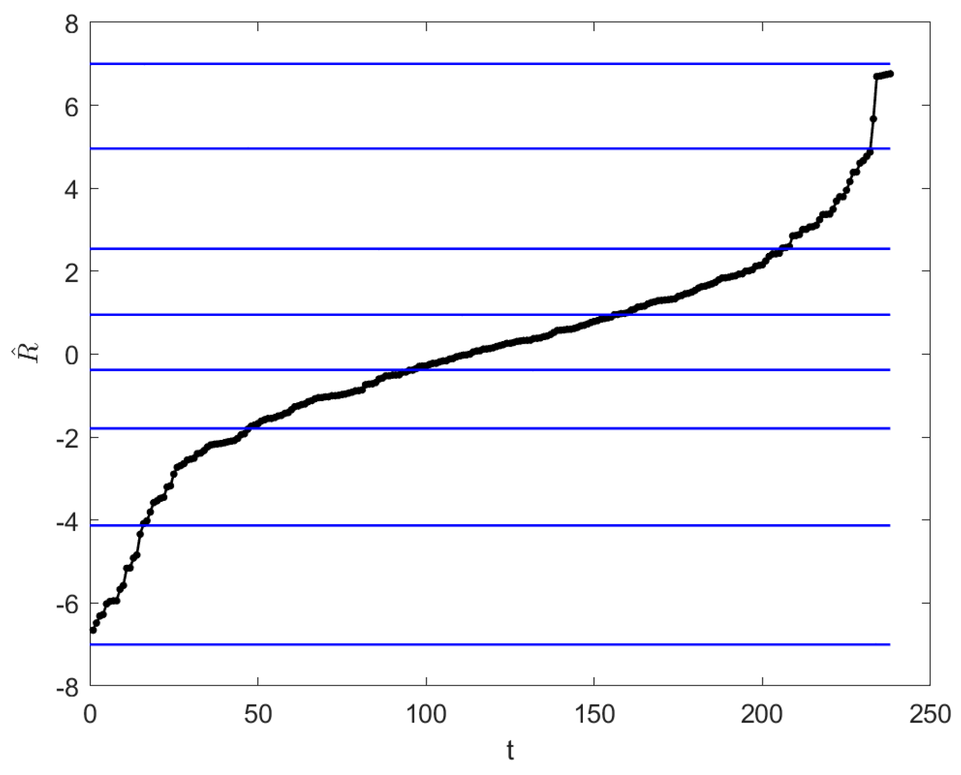
3.1. Initial Partition of the Universe of Discourse Based on FCM

Given a time series dataset $X=\{x_1,x_2,\dots ,x_n\}$, we define $X_{min}=\min \{x_i|x_i\in X\}$ and $X_{max}=\max \{x_i|x_i\in X\}$. Let $U=[U_l,U_u]=[X_{\min }-l_1,X_{\max }+l_2]$ denote the universe of discourse, l₁ and l₂ are called trimming factors, which are two appropriate positive numbers. Assume the universe is partitioned into p intervals (typically p > 2). We utilize the FCM method on the time series X to obtain the cluster prototypes V of the universe of discourse, which are denoted as the clustering centers. Then, we arrange these clustering centers in ascending order and calculate the medians of two adjacent clustering centers as the boundary values of the subintervals of the partitioned universe of discourse as follows:

$$h_i={\displaystyle \frac{c_i+c_{i+1}}{2}},i=1,2,\dots ,n-1$$

(18)

where h_i represents the boundary value of the partition, and c_i denotes the clustering center obtained by the FCM.

Then, the subintervals after initial partitioning are expressed as follows:

$$\begin{array}{l}{u}_1=\{x\in X|U_l\le x<h_1\}\\ u_2=\{x\in X|h_1\le x<h_2\}\\ ⋮\\ u_p=\{x\in X|h_{p-1}\le x\le U_u\}\end{array}$$

(19)

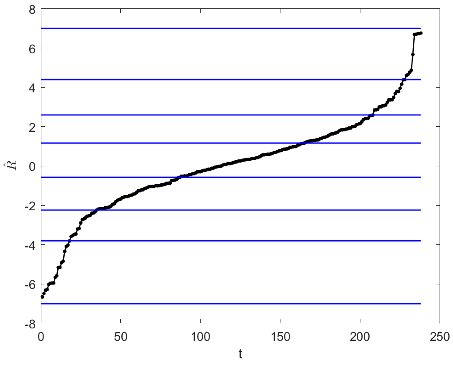
3.2. Optimized Partition of the Universe of Discourse Based on PJG and PSO

The subintervals after the initial partitioning of the universe of discourse are regarded as information granules, and we use triangular fuzzy sets to describe the information granules. The parameters of the information granules are related to the level of information granularity.

Given a subinterval set $X_i=\{-6.5,-8,1.2,-3.4,0.6,2.1,-2.3,3.7,4.5,5,-1.6\}$, we need to represent it with triangular fuzzy information granule. The specific solution steps are as follows:

(1) Sort X_i from smallest to largest to obtain the value of m.

After sorting X_i, we get $\stackrel{\wedge }{X_i}=\{-8,-6.5,-3.4,-2.3,-1.6,0.6,1.2,2.1,3.7,4.5,5\}$. If m = 0.6 is the median of X_i, then $\stackrel{\wedge }{X_i}$ is divided into two parts: $\stackrel{\wedge }{X_i^l}=\{-8,-6.5,-3.4,-2.3,-1.6\}$ and $\stackrel{\wedge }{X_i^r}=\{1.2,2.1,3.7,4.5,5\}$. $\stackrel{\wedge }{X_i^l}$ is used to solve the lower bound a, and $\stackrel{\wedge }{X_i^r}$ is used to solve the upper bound b.

(2) Assume that the information granularity level α = 0.5, and solve for the optimal lower bound $a_{opt}^{0.5}$ and the optimal upper bound $b_{opt}^{0.5}$ under this information granularity level.

First, solve the optimal lower bound $a_{opt}^{0.5}$ according to $\stackrel{\wedge }{X_i^l}$ and Formula (17).

$$a_i=-8,V(a_i^{0.5})=5\times \exp (-0.5\times |-8-0.6|)=0.0678$$

$$a_i=-6.5,V(a_i^{0.5})=4\times \exp (-0.5\times |-6.5-0.6|)=0.1149$$

$$a_i=-3.4,V(a_i^{0.5})=3\times \exp (-0.5\times |-3.4-0.6|)=0.4060$$

$$a_i=-2.3,V(a_i^{0.5})=2\times \exp (-0.5\times |-2.3-0.6|)=0.4691$$

$$a_i=-1.6,V(a_i^{0.5})=1\times \exp (-0.5\times |-1.6-0.6|)=0.3329$$

As a result, we obtain $a_{opt}^{0.5}=-2.3$. Likewise, we determine the optimal upper bound $b_{opt}^{0.5}$ according to $\stackrel{\wedge }{X_i^r}$ and Formula (17).

$$b_i=1.2,V(b_i^{0.5})=1\times \exp (-0.5\times |1.2-0.6|)=0.7408$$

$$b_i=2.1,V(b_i^{0.5})=2\times \exp (-0.5\times |2.1-0.6|)=0.9447$$

$$b_i=3.7,V(b_i^{0.5})=3\times \exp (-0.5\times |3.7-0.6|)=0.6367$$

$$b_i=4.5,V(b_i^{0.5})=4\times \exp (-0.5\times |4.5-0.6|)=0.5691$$

$$b_i=5,V(b_i^{0.5})=5\times \exp (-0.5\times |5-0.6|)=0.5540$$

As a result, we obtain $b_{opt}^{0.5}=2.1$. In summary, at the information granularity level α = 0.5, we obtain the optimal triangular fuzzy information granule ${\mathrm{\Omega }}^{0.5}=[-2.3,2.1]$.

Since $\alpha \in [0,1]$, the optimal information granule Ω^α will change as α varies, as shown in

Table 1. Ω^α of different α.

α	Ωα	α	Ωα
0	[−8,5]	0.6	[−2.3,2.1]
0.1	[−8,5]	0.7	[−2.3,2.1]
0.2	[−3.4,5]	0.8	[−2.3,1.2]
0.3	[−3.4,5]	0.9	[−2.3,1.2]
0.4	[−2.3,2.1]	1	[−1.6,1.2]
0.5	[−2.3,2.1]

.

For each subinterval X_i, its information granule ${\mathrm{\Omega }}_i^{\alpha }$ can be determined through the above fuzzy information granulation operation. In order to make the divided intervals have clearer semantic characteristics, we introduce the following indicator to describe the information granules constructed in the current interval:

$$Vol({\mathrm{\Omega }}_i)=|h_i-h_{i-1}|{\int }_0^1|{\mathrm{\Omega }}_i^{\alpha }|da=d_i{\int }_0^1|{\mathrm{\Omega }}_i^{\alpha }|da$$

(20)

where $d_i=|h_i-h_{i-1}|$ is the width of the interval X_i, and $|{\mathrm{\Omega }}_i^{\alpha }|=|b_i^{\alpha }-a_i^{\alpha }|$ represents the size of the constructed information granule. From Formula (20), it can be seen that the evaluation of the partitioned intervals takes into account the information granule ${\mathrm{\Omega }}_i^{\alpha }(\alpha =0,0.1,\dots ,1)$ at all levels of information granularity, rather than considering the information granules at a single level of information granularity.

Still taking the above dataset X_i as an example, based on the information granules formed under different levels of information granularity, we calculate the value of $|{\mathrm{\Omega }}^{\alpha }|=|b^{\alpha }-a^{\alpha }|$, as shown in Figure 2. The solution process of ${\int }_0^1|{\mathrm{\Omega }}_i^{\alpha }|da$ is as follows:

As shown in Figure 2, as the information granularity level α increases, the corresponding information granule size ${\displaystyle |{\mathrm{\Omega }}^{\alpha }|}$ is constantly decreasing, and its changing trend is in a polyline shape. Therefore, solving for ${\displaystyle {\int }_0^1|{\mathrm{\Omega }}_i^{\alpha }|}d\alpha$ can be transformed into calculating the sum of the integrals of several piecewise linear functions. The evaluation indicator for the information granulation of the entire dataset X is as follows:

$$V=Vol({\mathrm{\Omega }}_1)+Vol({\mathrm{\Omega }}_2)+\dots +Vol({\mathrm{\Omega }}_p)$$

(21)

Since the value of V varies with each subinterval X_i, the optimization problem for the partitioning of the universe of discourse is thus transformed into the following optimization problem [41]:

$${\min }_{d_1,d_2,\dots ,d_p}{\displaystyle \sum _{i=1}^{p}Vol({\mathrm{\Omega }}_i)}$$

(22)

For this optimization problem, we select the PSO algorithm to derive the optimal partitioning intervals of the universe of discourse. Among them, the initial solution is the initial partitioning intervals of the universe of discourse using the FCM algorithm.

In summary, we propose a partition algorithm of the universe of discourse based on FCM, PJG, and PSO.

In Algorithm 1, we first apply the FCM algorithm to partition a time series consisting of n points into p clusters, obtaining the initial partition intervals. If the number of iterations for the FCM algorithm is N₁, the time complexity is O(p²nN₁). Secondly, we calculate the information granule representation at each level of information granularity according to the PJG, with a time complexity of approximately O(n). Finally, we construct the objective function based on Formulas (21) and (22) and solve it using the PSO algorithm. Assuming the number of iterations for the PSO algorithm is N₂, the time complexity is O(pnN₂). Therefore, the overall time complexity of Algorithm 1 is O(p²nN₁ + n + pnN₂).

Algorithm 1: Partition of the Universe of Discourse Based on FCM, PJG, and PSO

Input: Time series $X=\{x_1,x_2,\dots ,x_n\}$ and the number of partition intervals p Output: The optimal partition intervals of the universe of discourse $U=\{u_1,u_2,\dots ,u_p\}$

1. Utilize the FCM clustering method to divide the universe of discourse into p clusters, obtain the clustering centers, then sort the clustering centers in ascending order, and calculate the initial partition subintervals of the universe of discourse according to Formula (19). 2. For the initial partition subintervals, use triangular fuzzy sets to construct information granules $\mathrm{\Omega }=[a,m,b]$, and solve the parameters of TFIGs according to PJG. 3. For the TFIGs, use the PSO algorithm to solve it according to Formulas (21) and (22) to obtain the final optimal partition intervals $U=\{u_1,u_2,\dots ,u_p\}$ of the universe of discourse.

4. Fuzzy Time Series Forecasting Based on the Novel Partition of the Universe of Discourse

The fuzzy time series forecasting model usually contains four basic steps: (1) defining and partitioning the universe of discourse; (2) defining fuzzy sets and fuzzifying historical time series; (3) establishing fuzzy logical relationships of the fuzzy time series; (4) forecasting and defuzzifying the fuzzy time series. Utilizing the optimal partitioning results of the universe of discourse from Section 3, the framework for fuzzy time series forecasting is presented in Figure 3.

The exact steps of the fuzzy time series forecasting based on the optimal partition of the discourse universe are presented in this section using the Taiwan Stock Exchange Capitalization Weighted Stock Index (TAIEX) as an example. Among them, the data from 4 January 1991 to 30 October 1991, spanning the first ten months, is designated as the training set, while the data from 1 November 1991 to 28 December 1991, covering the last two months, is used as the test set.

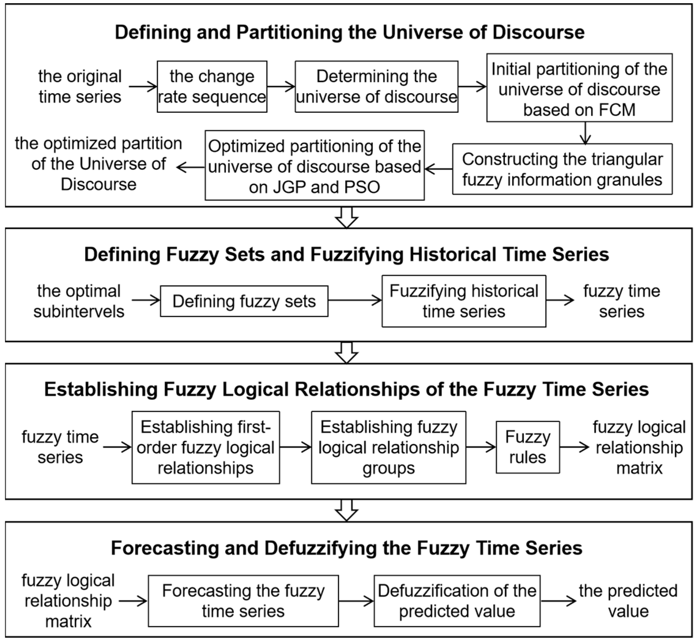
4.1. Defining and Partitioning the Universe of Discourse

Step 1: Converting the original time series into a rate of change series.

$$R(t)={\displaystyle \frac{x(t)-x(t-1)}{x(t-1)}}\times 100$$

(23)

where R(t) denotes the rate of change of the stock index on the t-th trading day, x(t) is the stock index at the current moment, and x(t − 1) is the stock index at the previous moment.

The original stock index time series can be transformed into a stock index change rate sequence using Formula (23).

Table 2. The original time series and the change rate sequence of the TAIEX training set.

Time	The Original Data	The Rate of Change (%)	Time	The Original Data	The Rate of Change (%)
03/01/1991	4258	-	02/07/1991	5613	−2.69
04/01/1991	4367	2.56	03/07/1991	5604	−0.16
05/01/1991	4456	2.04	04/07/1991	5607	0.05
07/01/1991	4191	−5.95	05/07/1991	5591	−0.29
08/01/1991	3975	−5.15	06/07/1991	5412	−3.20
$⋮$	$⋮$	$⋮$		$⋮$	$⋮$
25/06/1991	5872	−3.58	23/10/1991	4135	1.15
26/06/1991	6023	2.57	24/10/1991	4253	2.85
27/06/1991	5931	−1.53	28/10/1991	4381	3.01
28/06/1991	5900	−0.52	29/10/1991	4364	−0.39
29/06/1991	5768	−2.24	30/10/1991	4389	0.57

and Figure 4 show the original time series and the transformed change rate sequence of the TAIEX training set.

Obviously, the transformed sequence has removed the influence of trends and is more convenient for subsequent operation and processing [42].

Step 2: Determining the universe of discourse.

Define the universe of discourse $U=[U_l,U_u]=[r_{\min }-l_1,r_{\max }+l_2]$, where r_min represents the minimum value of the sequence R, r_max denotes the maximum value of the the sequence R, and l₁ and l₂ are called trimming factors, which are two appropriate positive numbers.

For the above change rate sequence, its minimum and maximum values are r_min = −6.66 and r_max = 6.76, respectively. Therefore, we set the trimming factors to l₁ = 0.34 and l₂ = 0.24, resulting in the universe of discourse $U=[-7,7]$ to be partitioned.

Step 3: Dividing the universe of discourse.

Step 3.1: Initial partitioning of the universe of discourse based on FCM.

Many scholars have already conducted research on TAIEX datasets, dividing the universe of discourse into seven intervals [23], which can yield relatively high-quality and strongly interpretable forecasting results. Therefore, in this study, we also assume that the number of fuzzy intervals is seven, and the number of clustering centers is seven. We subsequently perform the FCM method on the change rate sequence R(t) to obtain the cluster centers. After that, we sort the cluster centers in ascending order and calculate the median of each pair of adjacent cluster centers to serve as the boundary values for dividing the universe of discourse into subintervals, resulting in the following subintervals: u₁ = [−7.00, −4.13), u₂ = [−4.13, −1.79), u₃ = [−1.79, −0.38), u₄ = [−0.38, 0.95), u₅ = [0.95, 2.54), u₆ = [2.54, 4.96), u₇ = [4.96, 7.00].

As shown in Figure 5, the subintervals using FCM are consistent with the distribution characteristics of the data points. In areas with dense data distribution, the intervals of the divided subintervals are smaller, whereas in areas with sparse data distribution, the intervals of the divided subintervals are larger. However, the number of data points within each subinterval differs significantly. Specifically, subintervals with dense data distribution have many data points, whereas those with sparse data distribution have few data points. Therefore, it is necessary to optimize the current subintervals.

Step 3.2: Optimized partitioning of the universe of discourse based on PJG and PSO.

Taking the subintervals obtained in the previous step as the initial solution, we optimize them using the PSO algorithm, and the objective function is ${\min }_{d_1,d_2,\dots ,d_7}{\displaystyle \sum _{i=1}^{7}Vol({\mathrm{\Omega }}_i)}$, resulting in the following optimized subintervals: $u_1^{\prime }=[-7.00,-3.80)$, $u_2^{\prime }=[-3.80,-2.24]$, $u_3^{\prime }=[-2.24,-0.57)$, $u_4^{\prime }=[-0.57,1.17]$, $u_5^{\prime }=[1.17,2.60)$, $u_6^{\prime }=[2.60,4.40)$, $u_7^{\prime }=[4.40,7.00]$.

As illustrated in Figure 6, the subintervals derived from the optimized partitioning algorithm based on PJG and PSO exhibit clearer data point distribution features compared to those from the initial partitioning method shown in Figure 5. Moreover, the optimized subintervals show a more balanced distribution of data point quantities.

4.2. Defining Fuzzy Sets and Fuzzifying Historical Time Series

Step 1: Defining fuzzy sets based on the optimized partition.

Based on the partition subintervals obtained in Section 4.1, we define fuzzy sets for each subinterval as $A_1,A_2,\dots ,A_7$, where each fuzzy set is determined as a semantic value, as shown in

Table 3. Subintervals, fuzzy sets, and semantic values.

Subinterval	Fuzzy Set	Semantic Value
[−7.00, −3.80)	A1	Sharp decrease
[−3.80, −2.24)	A2	Decrease
[−2.24, −0.57)	A3	Slight decrease
[−0.57, 1.17)	A4	No change
[1.17, 2.60)	A5	Slight increase
[2.60, 4.40)	A6	Increase
[4.40, 7.00]	A7	Sharp increase

.

Then, we define fuzzy sets on U, and each Ai is expressed in terms of the subintervals $A_1,A_2,\dots ,A_7$.

$$\begin{array}{l}{A}_1=1/u_1+0.5/u_2+0/u_3+\dots +0/u_7\\ A_2=0.5/u_1+1/u_2+0.5/u_3+\dots +0/u_7\\ ⋮\\ A_6=0/u_1+0/u_2+\dots +1/u_6+0.5/u_7\\ A_7=0/u_1+0/u_2+\dots +0.5/u_6+1/u_7\end{array}$$

Step 2: Fuzzifying historical time series.

According to the fuzzy set definitions in Step 1, we perform fuzzification on historical time series. When fuzzifying, the “maximum membership principle” is adopted, which means choosing the fuzzy set with the maximum membership degree corresponding to the sequence value as the fuzzy description of that data point. If the value of the data point belongs to the subinterval u_i, then the data point is fuzzified as A_i.

Table 4. Fuzzy values of some data of the change rate sequence.

Time	The Rate of Change (%)	Fuzzy Value	Time	The Rate of Change (%)	Fuzzy Value
03/01/1991	-	-	02/07/1991	−2.69	A2
04/01/1991	2.56	A5	03/07/1991	−0.16	A4
05/01/1991	2.04	A5	04/07/1991	0.05	A4
07/01/1991	−5.95	A1	05/07/1991	−0.29	A4
08/01/1991	−5.15	A1	06/07/1991	−3.20	A2
$⋮$	$⋮$	$⋮$	$⋮$	$⋮$	$⋮$
25/06/1991	−3.58	A2	23/10/1991	1.15	A4
26/06/1991	2.57	A5	24/10/1991	2.85	A6
27/06/1991	−1.53	A3	28/10/1991	3.01	A6
28/06/1991	−0.52	A4	29/10/1991	−0.39	A4
29/06/1991	−2.24	A3	30/10/1991	0.57	A4

presents the fuzzification results for some data points of the change rate sequence.

4.3. Establishing Fuzzy Logical Relationships

Step 1: Establishing first-order fuzzy logical relationships.

Leveraging the fuzzified data in Section 4.2, we establish first-order fuzzy logical relationships (FLRs). Assume that the fuzzy values at time t − 1 and t are A_i and A_j, respectively, then the resulting first-order FLR is A_i → A_j. The first-order FLRs of some data of the rate change sequence in Table 4 are shown in

Table 5. The first-order FLRs of some data of the rate change sequence.

Time	Fuzzy Value	First-Order FLR	Time	Fuzzy Value	First-Order FLR
03/01/1991	-	-	02/07/1991	A2	A3 → A2
04/01/1991	A5	-	03/07/1991	A4	A2 → A4
05/01/1991	A5	A5 → A5	04/07/1991	A4	A4 → A4
07/01/1991	A1	A5 → A1	05/07/1991	A4	A4 → A4
08/01/1991	A1	A1 → A1	06/07/1991	A2	A4 → A2
⋮	⋮	⋮	⋮	⋮	⋮
25/06/1991	A2	A3 → A2	23/10/1991	A4	A1 → A4
26/06/1991	A5	A2 → A5	24/10/1991	A6	A4 → A6
27/06/1991	A3	A5 → A3	28/10/1991	A6	A6 → A6
28/06/1991	A4	A3 → A4	29/10/1991	A4	A6 → A4
29/06/1991	A3	A4 → A3	30/10/1991	A4	A4 → A4

.

Step 2: Establishing first-order fuzzy logical relationships.

Merging FLRs with the same antecedent into the same group, we can establish a fuzzy logical relationship group (FLRG). Assuming the existence of FLRs A_i → A_j and A_i → A_z, we then construct the FLRG: A_i → A_j, A_z. Utilizing the partial first-order FLRs listed in Table 5, we obtain the first-order FLRGs shown in

Table 6. Partial first-order FLRGs.

FLRGs
$A_1\to A_1,A_4$	$A_4\to A_2,A_3,A_4,A_6$	$A_1\to A_1,A_4$
$A_2\to A_4,A_5$	$A_5\to A_1,A_3,A_5$	$A_2\to A_4,A_5$
$A_3\to A_2,A_4$	$A_6\to A_4,A_6$	$A_3\to A_2,A_4$

.

Utilizing the derived FLRGs, we can formulate fuzzy rules. The expression for the fuzzy rules of the first-order FLR is presented as follows:

Rule R_i: If F_t−1 is A_i then F_t is A_j.

Step 3: Establishing the fuzzy logical relationship matrix.

Leveraging the FLRGs established in Step 2, we calculate the occurrence frequency of each fuzzy rule and establish the fuzzy logical relationship matrix, which is depicted in

Table 7. Fuzzy logical relationship matrix of occurrence frequency.

Ft−1	Ft
	A1	A2	A3	A4	A5	A6	A7
A1	3	1	3	6	3	1	1
A2	0	0	4	9	3	0	0
A3	5	4	11	16	8	7	2
A4	5	7	17	27	12	6	3
A5	4	2	7	13	13	3	1
A6	0	1	9	5	2	2	1
A7	1	1	2	2	1	1	2

.

Convert the occurrence frequencies in the above fuzzy logical relationship matrix into frequencies with the formula given below:

$$w_i(t)=[w_1^{\prime },w_2^{\prime },\dots ,w_m^{\prime }]=\left[{\displaystyle \frac{w_1}{{\displaystyle {\sum }_{j=1}^m{w}_j}}},{\displaystyle \frac{w_2}{{\displaystyle {\sum }_{j=1}^m{w}_j}}},\dots ,{\displaystyle \frac{w_m}{{\displaystyle {\sum }_{j=1}^m{w}_j}}}\right]$$

(24)

Calculate the frequencies according to Formula (24) to obtain the following weight matrix of fuzzy logical relationships, which is presented in

Table 8. Fuzzy logical relationship matrix of frequency.

Ft−1	Ft
	A1	A2	A3	A4	A5	A6	A7
A1	0.17	0.05	0.17	0.34	0.17	0.05	0.05
A2	0	0	0.25	0.56	0.19	0	0
A3	0.09	0.08	0.21	0.30	0.15	0.13	0.04
A4	0.06	0.09	0.22	0.35	0.16	0.08	0.04
A5	0.09	0.05	0.16	0.30	0.30	0.08	0.02
A6	0	0.05	0.45	0.25	0.10	0.10	0.05
A7	0.10	0.10	0.20	0.20	0.10	0.10	0.20

.

4.4. Forecasting and Defuzzification

Step 1: Forecasting the fuzzy time series.

After establishing the fuzzy logical relationship matrix for historical time series, we can predict the future time series with the formula provided below:

$$R(t)=M_{df}\times w_i(t-1)$$

(25)

where R(t) indicates the predicted change rate value at time t; $M_{df}=[m_1,m_2,\dots ,m_h]$ denotes the defuzzification matrix; $m_1,m_2,\dots ,m_h$ represent the mid-values of the corresponding subintervals, respectively; and $w_i(t-1)$ is the weight vector of the fuzzy logical relationship matrix.

Step 2: Defuzzification of the predicted value.

Translate the predicted stock index rate of change into the final stock index prediction value according to Formula (26):

$$x(t)=x(t-1)\times (1+R(t))$$

(26)

where x(t) signifies the forecasted stock index value at time t, while x(t − 1) corresponds to the actual stock index value at the previous moment.

By performing calculations according to Formulas (25) and (26), we obtain the predicted values for the test set of TAIEX. As depicted in Figure 7, the actual values and the predicted values exhibit a fundamentally consistent trend.

In sum, we propose the fuzzy time series forecasting algorithm based on the optimized partition of the universe of discourse, outlined below.

In Algorithm 2, we integrate Algorithm 1 into the prediction framework of fuzzy time series to forecast the time series. By simply inputting the time series X and the number of partition intervals p of the universe of discourse, we can obtain the predicted value x(t).

Algorithm 2: Fuzzy Time Series Forecasting Based on the Novel Partition of the Universe of Discourse

Input: Time series $X=\{x_1,x_2,\dots ,x_n\}$ and the subintervals p Output: Predicted value x(t)

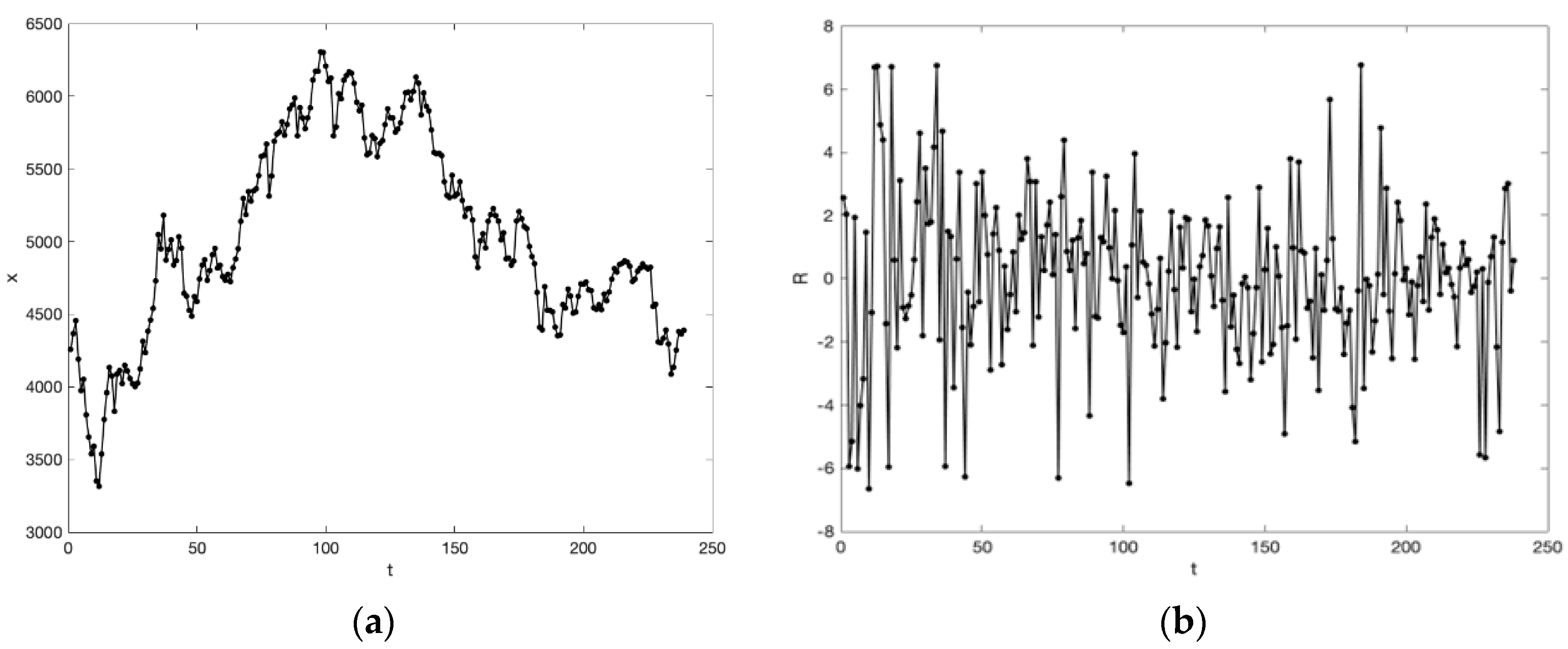
1. Define and partition the universe of discourse. Convert the original time series X into a rate of change series R, and define the universe of discourse of R is $U=[U_l,U_u]=[r_{\min }-l_1,r_{\max }+l_2]$, then use Algorithm 1 to divide U into p subintervals. 2. Define fuzzy sets and fuzzify historical time series. Based on the subintervals, define a fuzzy set for each subinterval, and fuzzify the historical data to obtain the fuzzy time series. 3. Establish fuzzy logical relationships. Based on the fuzzified data, establish fuzzy logical relationships. Combine the FLRs with the same antecedents into the same group to construct fuzzy logical relationship groups, thereby obtaining fuzzy logic rules and building the fuzzy logical relationship matrix. 4. Perform forecasting and defuzzification. For the fuzzy logical relationship matrix, calculate the fuzzy predicted values according to Formula (25), and perform defuzzification according to Formula (26) to derive the final predicted value x(t).

5. Experiments

To illustrate the effectiveness of the suggested forecasting method, a few experiments are conducted in this section using MATLAB R2022a. The experimental data are selected from the Taiwan Weighted Stock Index (TAIEX) dataset and the Shanghai Composite Index (SHCI) dataset. In Section 5.1, the Root Mean Square Error (RMSE) and Linguistic Accuracy (LA) are used as performance measures to evaluate the forecasting accuracy of the suggested approach. To compare the accuracy of the prediction results of the suggested technique with those of analogous algorithms in the body of existing research, tests are conducted using the TAIEX datasets in Section 5.2. The SHCI datasets are utilized for real-world application research in Section 5.3.

5.1. Evaluation Metrics

5.1.1. Evaluation Metric of Prediction Accuracy

To measure the prediction accuracy of the proposed model, the Root Mean Square Error (RMSE) is chosen as the evaluation metric, which calculates the deviation between the actual values and the predicted values. The calculation formula is as follows:

$$RMSE=\sqrt{{\displaystyle \frac{{\displaystyle {\sum }_{t=1}^n{(x_{fv}(t)-x_{av}(t))}^2}}{n}}}$$

(27)

where n represents the size of the test set, $x_{fv}(t)$ is the predicted value at time t, and $x_{av}(t)$ is the actual value at time t. A smaller RMSE value signifies that the predicted values are closer to the actual values, reflecting the higher accuracy of the model’s predictions.

5.1.2. Evaluation Metric of Predicted Linguistic Accuracy

To evaluate the model’s performance in semantic prediction, we use the Linguistic Accuracy (LA) [43] as the assessment metric to measure the difference between the predicted and genuine linguistic values. The following is the formula for computation.

$$\begin{gathered} LA(\%)={\displaystyle \sum _{t=1}^N\frac{g(t)}{N}}\times 100 \\ g(t)=\{\begin{array}{l}1,\mathrm{if}{\widehat{L}}_t=L_t\\ 0,\mathrm{if}{\widehat{L}}_t\ne L_t\end{array} \end{gathered}$$

(28)

where N denotes the total number of the dataset, $L_t$ represents the true linguistic value at time t, and ${\widehat{L}}_t$ indicates the predicted linguistic value at time t.

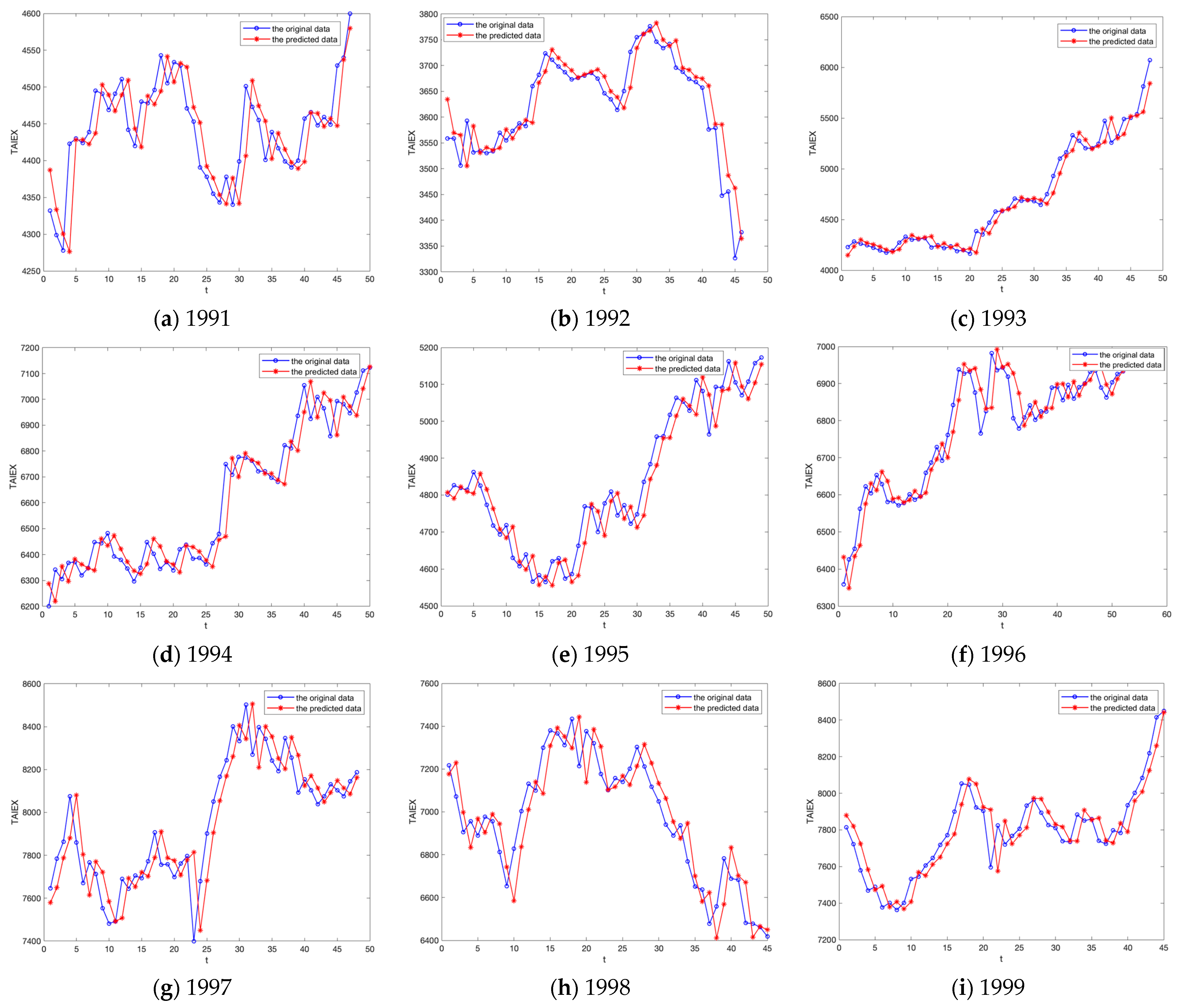
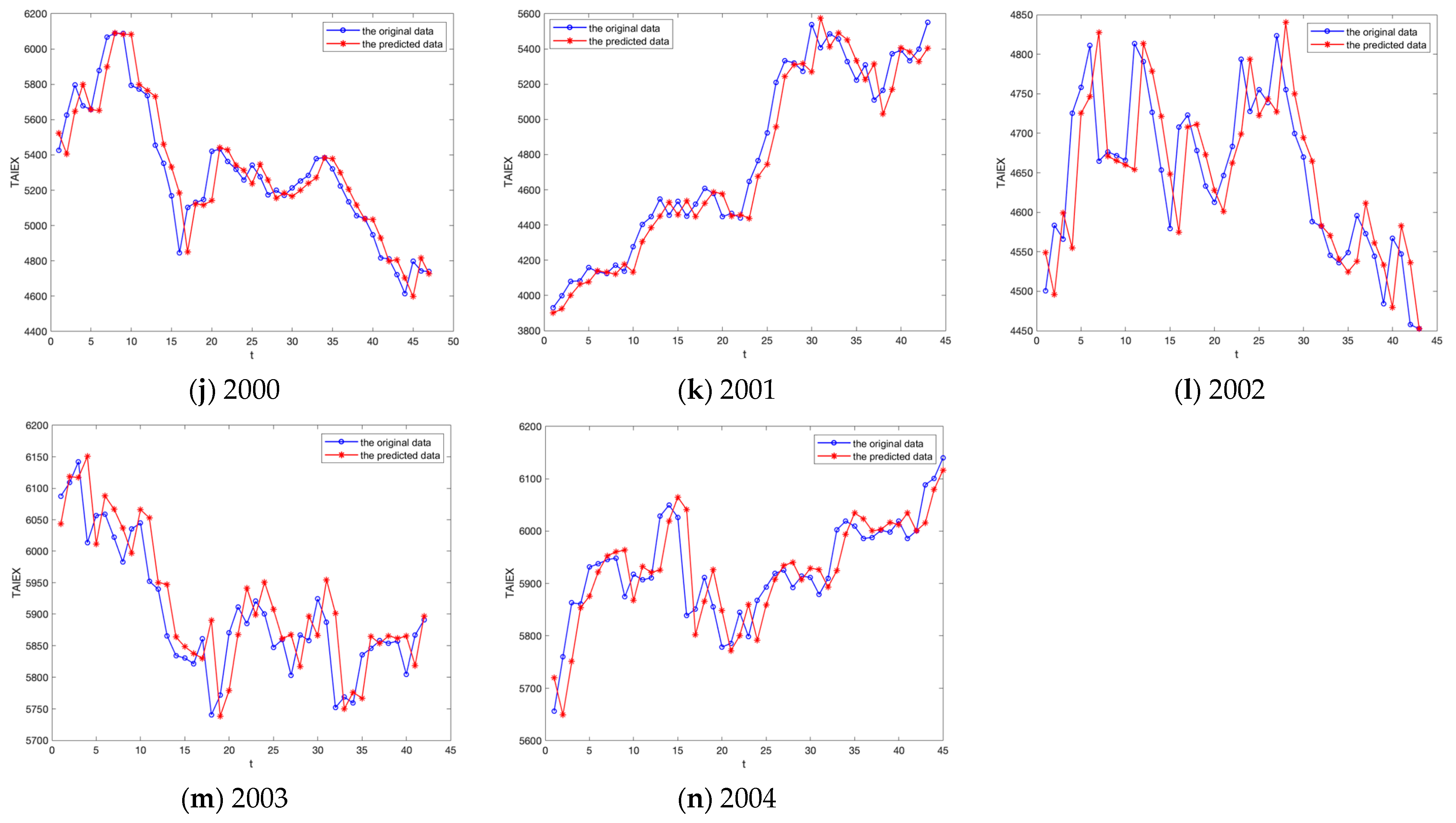
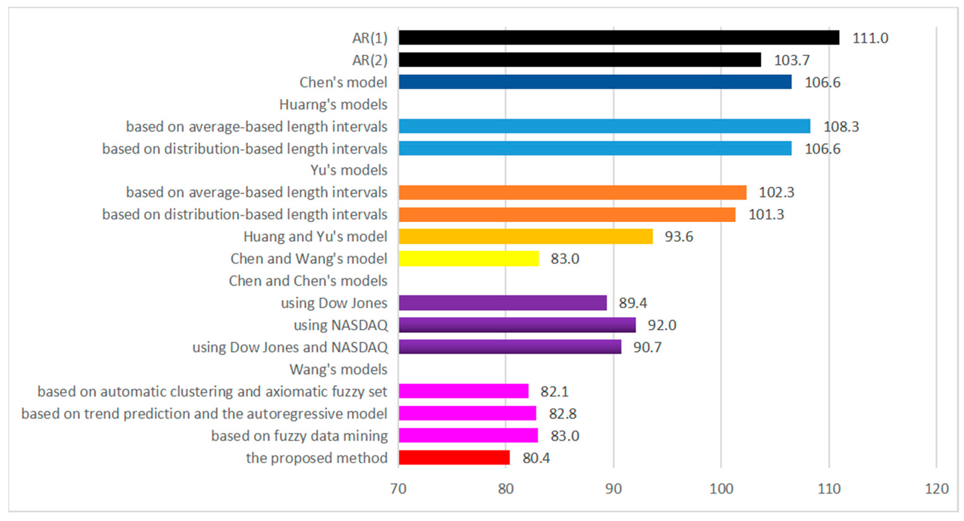
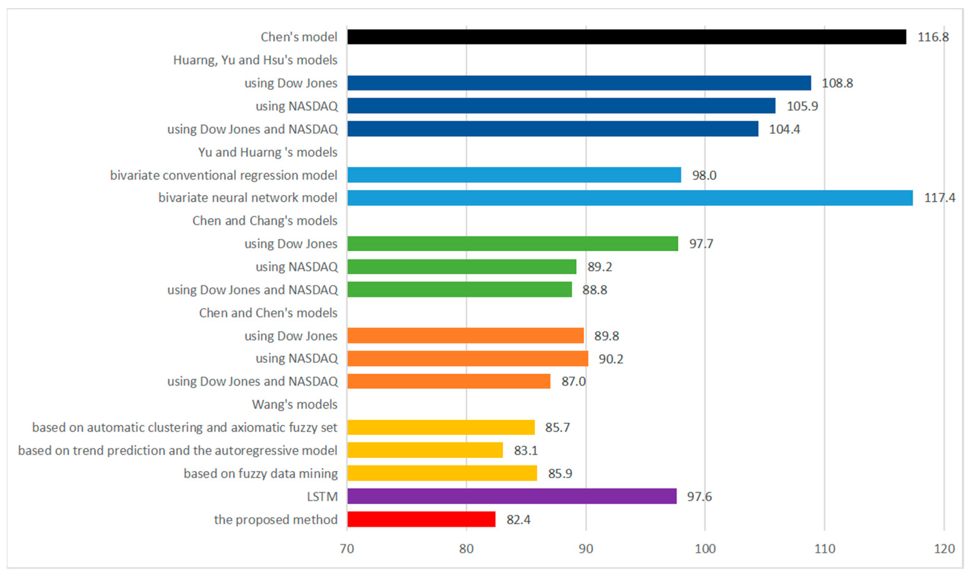
5.2. Experiment A: TAIEX Forecasting

The TAIEX datasets are frequently applied as experimental data for fuzzy time series forecasting models [43,44,45,46,47,48,49,50,51,52,53]. For experimentation and comparison with existing related prediction methods, 14 TAIEX datasets from 1991 to 2004 are selected in this section.

Each year’s TAIEX is treated as a dataset. The first ten months of each dataset are designated as the training set, while the final two months serve as the test set.

Table 9. Information on training and test sets for TAIEX from 1991 to 2004.

Year	Size	Training Set	Size of Training Set	Test Set	Size of Test Set
1991	286	1/3~10/30	239	11/1~12/28	47
1992	284	1/4~10/30	238	11/2~12/29	46
1993	291	1/5~10/30	243	11/2~12/31	48
1994	286	1/5~10/29	236	11/1~12/31	50
1995	286	1/5~10/30	237	11/1~12/30	49
1996	288	1/4~10/30	236	11/1~12/31	52
1997	286	1/4~10/30	238	11/3~12/31	48
1998	271	1/3~10/31	226	11/2~12/31	45
1999	266	1/5~10/30	221	11/1~12/28	45
2000	271	1/4~10/31	224	11/1~12/30	47
2001	244	1/2~10/31	201	11/1~12/31	43
2002	248	1/2~10/31	205	11/1~12/31	43
2003	248	1/2~10/31	206	11/3~12/31	42
2004	250	1/2~10/29	205	11/1~12/31	45

provides the information on training and test sets for TAIEX from 1991 to 2004.

In all experiments, the universe of discourse is divided into seven subintervals, with the parameters for the PSO algorithm listed in

Table 10. The parameters for the PSO algorithm in Experiment A.

Parameters	Value
Particle swarm size	150
Number of iterations	1000
Inertia weight coefficient	0.8
Cognitive coefficient	1.5
Social coefficient	1.5

.

The forecasting model developed in this research is used to conduct experiments on the datasets mentioned above. The test set is predicted by first processing the training set to extract the fuzzy logical relationships. Figure 8 illustrates the forecasting results.

Figure 8 shows how the TAIEX’s annual change trends vary from one another. In essence, the trend of the original data and the expected values produced by the suggested model match.

Since most of the existing research methods only use part of the TAIEX datasets from 1991 to 2004 for experiments, for the convenience of comparison with the existing research methods, we divide the TAIEX datasets from 1991 to 2004 into two parts for experiments. Experiment 1 uses the TAIEX datasets from 1991 to 1999, and Experiment 2 uses the TAIEX datasets from 2000 to 2004.

Table 11. RMSE comparison of the prediction models for TAIEX from 1991 to 1999.

Models	1991	1992	1993	1994	1995	1996	1997	1998	1999
AR(1) [44]	87.1	95.8	103.6	111.7	90.3	86	153.3	149.2	121.9
AR(2) [44]	59.2	76.9	110.9	111.1	69.2	62.9	175.3	137	130.9
Chen [45]	80	60	110	112	79	54	148	167	149
Huarng [46]
based on average-based length intervals	79.4	59.9	105.2	132.4	78.6	52.1	148.8	159.3	159.1
based on distribution-based length intervals	80.2	60.3	110	111.7	78.6	54.2	148.0	167.3	148.7
Yu [47]
based on average-based length intervals	61	67	105	135	70	54	133	151	145
based on distribution-based length intervals	67	56	105	114	70	52	152	154	142
Huang and Yu [48]	54.7	61.1	117.9	88.7	64.1	52.1	135.9	136.2	131.9
Chen and Wang [49]	42.9	43.5	103.4	89.8	52.2	52.8	140.8	116.9	104.9
Chen and Chen [50]
using Dow Jones	72.9	43.4	103.2	78.6	66.7	59.8	139.7	124.4	115.5
using NASDAQ	66.1	49.6	104.8	75.7	67.0	60.9	140.9	144.1	119.3
using Dow Jones and NASDAQ	74.9	43.8	101.4	78.1	68.1	61.3	139.3	132.9	116.6
Wang [51]
based on automatic clustering and axiomatic fuzzy set	43.6	41.4	102.4	89.0	55.0	49.4	139.0	118.2	100.9
based on trend prediction and the autoregressive model	42.5	44.0	101.0	93.1	52.9	50.5	145.1	115.1	101.3
based on fuzzy data mining	43.5	43.3	102.2	87.6	57.1	50.6	139.5	120.4	102.9
The proposed method	43.5	42.3	98.2	80.1	53.4	52.0	132.5	120.3	101.2

presents the RMSE comparison of the proposed model in this paper with other representative prediction models on the TAIEX datasets from 1991 to 1999. Among them, AR(1) and AR(2) [44] are classic time-series prediction models. Chen [45] introduced a traditional fuzzy time-series prediction model. Huarng [46], Yu [47], and Huarng and Yu [48] focused on partitioning the universe of discourse and determining sub-interval lengths to enhance prediction accuracy. Chen and Wang [49] emphasized extracting more effective fuzzy logical relationships from time series. Chen and Chen [50] concentrated on multi-factor fuzzy time-series prediction models using various strategies. Wang [51] developed several fuzzy theory-based time-series prediction models, including models based on automatic clustering and axiomatic fuzzy sets, trend prediction and autoregressive models, and fuzzy data mining.

To facilitate a more intuitive comparison of prediction accuracy among various methods, we computed the average RMSE for different prediction models applied to TAIEX data from 1991 to 1999. As depicted in Figure 9, the proposed model achieves an average RMSE of 80.4. This value is the lowest among the compared methods, signifying superior prediction accuracy.

Table 12. RMSE comparison of the prediction models for TAIEX from 2000 to 2004.

Models	2000	2001	2002	2003	2004
Chen [45]	176.3	147.8	101.2	74.5	84.3
Huarng, Yu and Hsu [52]
using Dow Jones	165.8	138.25	93.73	72.95	73.49
using NASDAQ	158.7	136.49	95.15	65.51	73.57
using Dow Jones and NASDAQ	157.64	131.98	93.48	65.51	73.49
Yu and Huarng [53]
bivariate conventional regression model	154	120	77	54	85
bivariate neural network model	274	131	69	52	61
Chen and Chang [54]
using Dow Jones	148.8	113.7	79.8	64.08	82.32
using NASDAQ	131.1	115.1	73.1	66.4	60.5
using Dow Jones and NASDAQ	130.1	113.3	72.3	60.3	68.1
Chen and Chen [50]
using Dow Jones	127.5	122.0	74.7	66.0	58.9
using NASDAQ	129.9	123.1	71.0	65.1	61.9
using Dow Jones and NASDAQ	123.6	123.9	71.9	58.1	57.7
Wang [51]
based on automatic clustering and axiomatic fuzzy set classification	138.0	113.8	65.0	56.5	55.3
based on trend prediction and the autoregressive model	132.0	111.5	65.3	52.4	54.2
based on fuzzy data mining	131.6	113.6	68.5	59.3	56.7
LSTM [9]	136	101	89	92	70
The proposed method	121.2	112.7	65.5	57.6	55.2

and Figure 10 offer a comparison of the RMSE values between the proposed model and other representative prediction models using the TAIEX datasets from 2000 to 2004.

As shown in Figure 10, the proposed model achieves an average RMSE value of 82.4, which is the lowest among all the prediction methods, indicating the highest prediction accuracy. Compared with Chen’s model [45]; Huarng, Yu, and Hsu’s model [52]; Yu and Huarng’s model [53]; Chen and Chang’s model [54]; Chen and Chen’s model [50]; Wang’s model [51]; and LSTM [9], the proposed model in this chapter has an absolute advantage in prediction accuracy.

The experiments clearly demonstrate that the proposed method in this article achieves higher prediction accuracy than existing models on the TAIEX datasets.

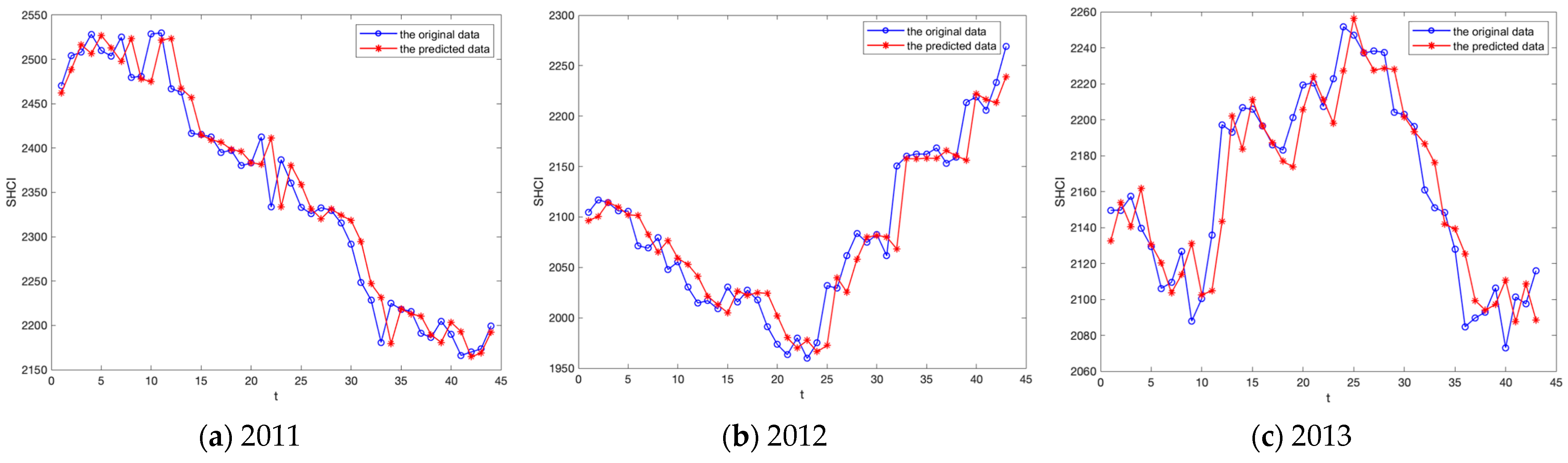
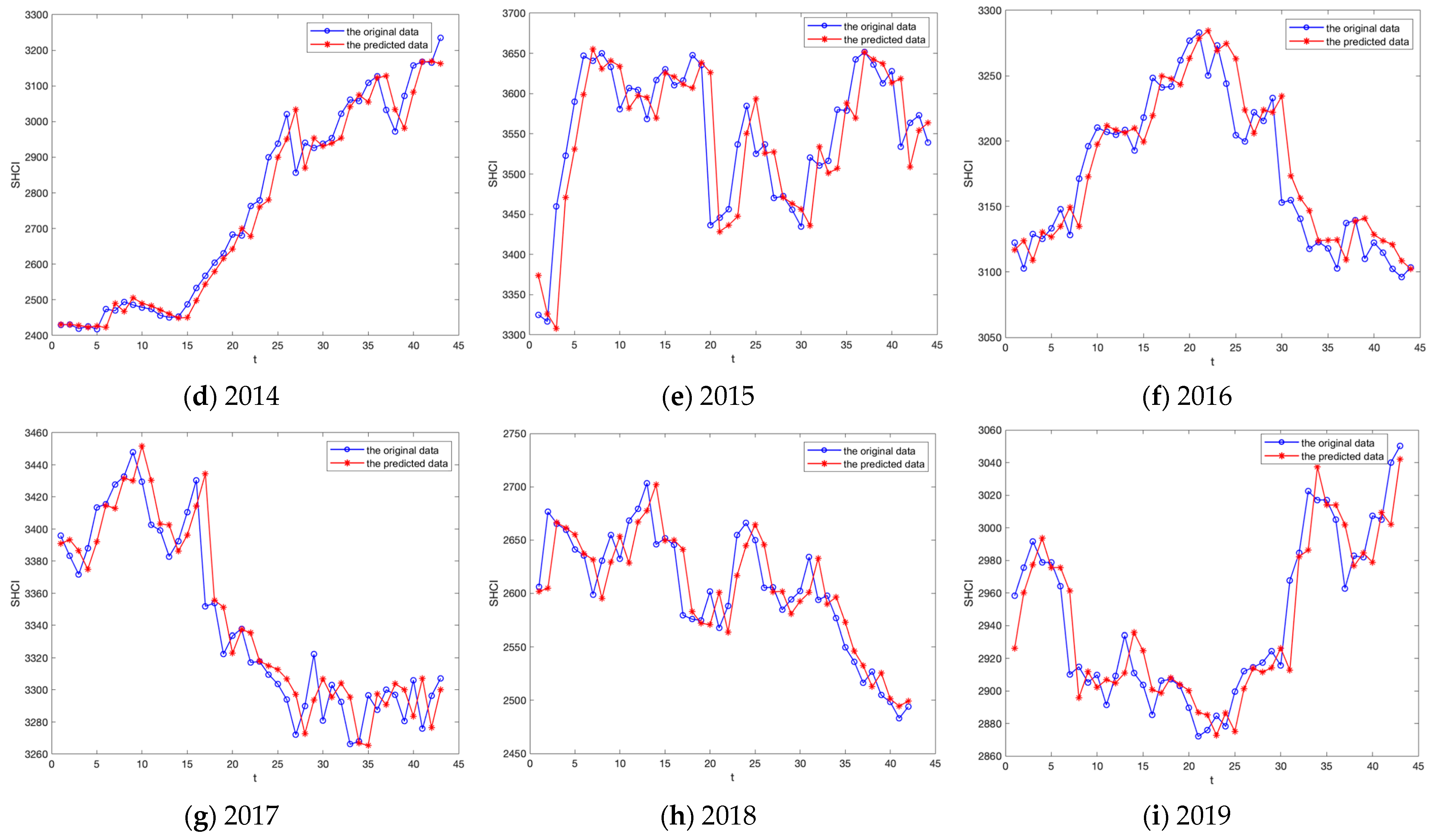
5.3. Experiment B: SHCI Forecasting

The Shanghai Stock Composite Index (SHCI) is a significant indicator of the overall fluctuations in China’s stock market. In this section, a total of 10 datasets of SHCI from 2011 to 2019 are selected as experimental data for practical application. Each year’s SHCI is considered a dataset. The initial ten months of the dataset are used for the training set, whereas the final two months are allocated for the test set.

Table 13. Information on training and test sets for TAIEX SHCI from 2010 to 2019.

Year	Size	Training Set	Size of Training Set	Test Set	Size of Test Set
2011	244	1/4~10/31	200	11/1~12/30	44
2012	243	1/4~10/31	200	11/1~12/31	43
2013	238	1/4~10/31	195	11/1~12/31	43
2014	245	1/2~10/31	202	11/3~12/31	43
2015	244	1/5~10/30	200	11/2~12/31	44
2016	244	1/4~10/31	200	11/1~12/30	44
2017	244	1/3~10/31	201	11/1~12/29	43
2018	243	1/2~10/31	201	11/1~12/28	42
2019	244	1/2~10/31	201	11/1~12/31	43

lists the information on the training and test sets for SHCI from 2011 to 2019. In all experiments, the universe of discourse is partitioned into seven subintervals, and the parameters for PSO are detailed in

Table 14. The parameters for the PSO algorithm in Experiment B.

Parameters	Value
Particle swarm size	150
Number of iterations	1000
Inertia weight coefficient	0.8
Cognitive coefficient	1.5
Social coefficient	1.5

.

Subsequently, we apply the proposed model to Experiment B, with the prediction results illustrated in Figure 11.

Figure 11 clearly shows that the trend of the predicted values generated by the proposed model aligns closely with the direction of the original datasets. We calculate the RMSE of the prediction results of SHCI from 2011 to 2019, as shown in

Table 15. RMSE of the proposed model for SHCI from 2010 to 2019.

Year	2011	2012	2013	2014	2015	2016	2017	2018	2019
RMSE	27.40	24.13	19.69	52.05	54.00	22.06	21.05	26.75	20.12

, and the average RMSE value is 29.69.

According to the prediction results, we transform the numerical predicted values into the corresponding semantic values. Then, we calculate the LA value of the prediction results, as shown in

Table 16. LA of the proposed model for SHCI from 2010 to 2019.

Year	2011	2012	2013	2014	2015	2016	2017	2018	2019
LA(%)	70.45	58.14	72.09	60.47	75.00	75.00	72.09	97.62	76.74

.

The proposed model achieves an average LA value of 73.07% for SHCI predictions from 2011 to 2019. Since the semantic value corresponds to the degree of increase or decrease in the change rate sequence of the stock index, the obtained average LA indicates that the proposed model can accurately predict the increased or decreased changes in about three-quarters of the dataset.

To discuss the impact of the number of partition intervals p on the forecasting accuracy of our method, we conduct experiments to calculate the RMSE values for different p values, as shown in

Table 17. RMSE of the proposed model with different number of partition intervals p for SHCI 2019.

p	3	4	5	6	7	8	9	10
RMSE	37.29	20.43	20.22	20.96	20.12	21.69	21.61	23.84

. It can be observed that the RMSE value is minimized when p = 7, indicating that the model’s forecasting accuracy is optimal. The RMSE value is maximized when p = 3, and the model’s accuracy begins to decline when p > 7. Therefore, the setting of p should not be too small, nor is it better when it is too large.

In summary, the proposed model in this paper can accurately forecast the rising and falling trends of the future stock market. Investors can adjust their investment strategies according to the forecasting results, thereby increasing returns and reducing risks.

6. Conclusions

In this article, we provide a new fuzzy time series forecasting model that integrates fuzzy C-means clustering, principle of justifiable granularity, and particle swarm optimization. Firstly, the FCM approach is employed to divide the universe of discourse, thereby obtaining the initial subinterval division. Next, triangular fuzzy information granules are created for the subintervals in accordance with the principle of justifiable granularity. Then, an objective function is defined for the entire universe of discourse, and the PSO algorithm is applied to achieve the final result of the optimal subinterval division. Based on the optimal partition results, we implement the framework of the fuzzy time series model for forecasting. Finally, this approach is applied to both the TAIEX and SHCI datasets, and its forecasting performance is evaluated by comparing the results with those of other methods. The experimental results demonstrate that the proposed model in this paper achieves higher forecasting accuracy than other models. It not only exhibits good numerical forecasting performance but also achieves good semantic forecasting performance. This paper focuses on improving the partitioning technique of the universe of discourse to enhance the forecasting accuracy of time series. The forecasting approach is grounded in the established framework of fuzzy time series, so the prediction accuracy is also limited by the processing of fuzzy relationships. In the future, we will consider improving the prediction framework of fuzzy time series to enhance forecasting accuracy. Furthermore, we plan to apply this method to multi-step forecasting in fuzzy time series and utilize it for time series data in other domains to achieve better forecasting outcomes.

References

1. Yao, Y.; Zhang, Z.Y.; Zhao, Y. Stock index forecasting based on multivariate empirical mode decomposition and temporal convolutional networks. Appl. Soft Comput. 2023, 142, 110356. [Google Scholar] [CrossRef]
2. Palash, W.; Akanda, A.S.; Islam, S. A data-driven global flood forecasting system for medium to large rivers. Sci. Rep. 2024, 14, 8979. [Google Scholar] [CrossRef] [PubMed]
3. Xie, W.; Liu, C.; Wu, W.-Z. A novel fractional grey system model with non-singular exponential kernel for forecasting enrollments. Expert Syst. Appl. 2023, 219, 119652. [Google Scholar] [CrossRef]
4. Meng, X.; Zhao, H.; Shu, T.; Zhao, J.H.; Wan, Q.L. Machine learning-based spatial downscaling and bias-correction framework for high-resolution temperature forecasting. Appl. Intell. 2024, 54, 8399–8414. [Google Scholar] [CrossRef]
5. Box, G.E.P.; Jenkins, G.M. Time Series Analysis: Forecasting and Control; Holden-Day: San Francisco, CA, USA, 1990. [Google Scholar]
6. Aasim, S.N.; Singh, A. Mohapatra, Data driven day-ahead electrical load forecasting through repeated wavelet transform assisted SVM model. Appl. Soft Comput. 2021, 111, 107730. [Google Scholar] [CrossRef]
7. Wei, X.K.; Li, Y.H.; Zhang, P.; Lu, J.M. Analysis and applications of time series forecasting model via support vector machines. Syst. Eng. Electron. 2005, 27, 529–532. (In Chinese) [Google Scholar]
8. Wibawa, A.P.; Utama, A.B.P.; Elmunsyah, H.; Pujianto, U.; Dwiyanto, F.A.; Hernandez, L. Time-series analysis with smoothed Convolutional Neural Network. J. Big Data 2022, 9, 44. [Google Scholar] [CrossRef]
9. Kirisci, M.; Cagcag Yolcu, O. A new CNN-based model for financial time series: TAIEX and FTSE stocks forecasting. Neural Process. Lett. 2022, 54, 3357–3374. [Google Scholar] [CrossRef]
10. Siami-Namini, S.; Tavakoli, N.; Namin, A.S. The performance of LSTM and BiLSTM in forecasting time series. In Proceedings of the 2019 IEEE International Conference on Big Data, Los Angeles, CA, USA, 9–12 December 2019. [Google Scholar]
11. Zhou, F.; Huang, Z.; Zhang, C. Carbon price forecasting based on CEEMDAN and LSTM. Appl. Energy 2022, 311, 118601. [Google Scholar] [CrossRef]
12. Zadeh, L.A. Fuzzy sets. Inf. Control 1965, 8, 338–353. [Google Scholar] [CrossRef]
13. Takagi, T.; Sugeno, M. Fuzzy Identification of Systems and its Applications to Modeling and Control. IEEE Trans. Syst. Man Cybern. 1985, 15, 116–132. [Google Scholar] [CrossRef]
14. Song, Q.; Chissom, B.S. Forecasting enrollments with fuzzy time series—Part I. Fuzzy Sets Syst. 1993, 54, 1–9. [Google Scholar] [CrossRef]
15. Song, Q.; Chissom, B.S. Forecasting enrollments with fuzzy time series—Part II. Fuzzy Sets Syst. 1994, 62, 1–8. [Google Scholar] [CrossRef]
16. Chen, S.M.; Wang, J.R. A Novel Fuzzy Time Series Forecasting Model Based on Optimal Partitioning of the Universe of Discourse. Fuzzy Sets Syst. 2000, 114, 159–175. [Google Scholar]
17. Song, Q.; Chissom, B.S. Fuzzy time series and its models. Fuzzy Sets Syst. 1993, 54, 269–277. [Google Scholar] [CrossRef]
18. Huarng, K. Effective Lengths of Intervals to Improve Forecasting in Fuzzy Time Series. Fuzzy Sets Syst. 2001, 123, 387–394. [Google Scholar] [CrossRef]
19. Huarng, K.; Yu, H.K. Ratio-Based Lengths of Intervals to Improve Fuzzy Time Series Forecasting. IEEE Trans. Syst. Man Cybern. Part B Cybern. 2006, 36, 328–340. [Google Scholar] [CrossRef]
20. Chen, S.M.; Hsu, C.C. A New Method to Forecast Enrollments Using Fuzzy Time Series. Int. J. Appl. Sci. Eng. 2004, 2, 234–244. [Google Scholar]
21. Chen, M.Y.; Chen, B.T. A Hybrid Fuzzy Time Series Model Based on Granular Computing for Stock Price Forecasting. Inf. Sci. 2015, 294, 227–241. [Google Scholar] [CrossRef]
22. Wang, L.; Liu, X.; Pedrycz, W. Effective Intervals Determined by Information Granules to Improve Forecasting in Fuzzy Time Series. Expert Syst. Appl. 2013, 40, 5673–5679. [Google Scholar] [CrossRef]
23. Wang, L.; Liu, X.; Pedrycz, W.; Shao, Y.Y. Determination of Temporal Information Granules to Improve Forecasting in Fuzzy Time Series. Expert Syst. Appl. 2014, 41, 3134–3142. [Google Scholar] [CrossRef]
24. Yin, Y.; Sheng, Y.; Qin, J. Interval type-2 fuzzy C-means forecasting model for fuzzy time series. Appl. Soft Comput. 2022, 129, 109574. [Google Scholar] [CrossRef]
25. Pedrycz, W.; Wang, X.M. Designing fuzzy sets with the use of the parametric principle of justifiable granularity. IEEE Trans. Fuzzy Syst. 2016, 24, 489–496. [Google Scholar] [CrossRef]
26. Moreno, J.E.; Sanchez, M.A.; Mendoza, O.; Rodríguez-Díaz, A.; Castillo, O.; Melin, P.; Castro, J.R. Design of an interval Type-2 fuzzy model with justifiable uncertainty. Inf. Sci. 2020, 513, 206–221. [Google Scholar] [CrossRef]
27. Zhang, B.; Pedrycz, W.; Wang, X.; Gacek, A. Design of Interval Type-2 Information Granules Based on the Principle of Justifiable Granularity. IEEE Trans. Fuzzy Syst. 2021, 29, 3456–3469. [Google Scholar] [CrossRef]
28. Castillo, O.; Castro, J.R.; Melin, P. A Methodology for Building of Interval and General Type-2 Fuzzy Systems Based on the Principle of Justifiable Granularity. J. Mult. Valued Log. Soft Comput. 2023, 40, 253–284. [Google Scholar]
29. Aladag, C.H.; Basaran, M.A.; Egrioglu, E.; Yolcu, U.; Uslu, V.R. Forecasting in High Order Fuzzy Times Series by Using Neural Networks to Define Fuzzy Relations. Expert Syst. Appl. 2009, 36, 4228–4231. [Google Scholar] [CrossRef]
30. Aladag, C.H.; Yolcu, U.; Egrioglu, E. A High Order Fuzzy Time Series Forecasting Model Based on Adaptive Expectation and Artificial Neural Networks. Math. Comput. Simul. 2010, 81, 875–882. [Google Scholar] [CrossRef]
31. Egrioglu, E.; Aladag, C.H.; Yolcu, U.; Uslu, V.R.; Basaran, M.A. Finding an Optimal Interval Length in High Order Fuzzy Time Series. Expert Syst. Appl. 2010, 37, 5052–5055. [Google Scholar] [CrossRef]
32. Kuo, I.H.; Horng, S.J.; Chen, Y.H.; Run, R.S.; Kao, T.W.; Chen, R.J.; Lai, J.L.; Lin, T.L. Forecasting TAIFEX Based on Fuzzy Time Series and Particle Swarm Optimization. Expert Syst. Appl. 2010, 37, 1494–1502. [Google Scholar] [CrossRef]
33. Huang, Y.L.; Horng, S.J.; He, M.; Fan, P.; Kao, T.W.; Khan, M.K.; Lai, J.L.; Kuo, I.H. A Hybrid Forecasting Model for Enrollments Based on Aggregated Fuzzy Time Series and Particle Swarm Optimization. Expert Syst. Appl. 2011, 38, 8014–8023. [Google Scholar] [CrossRef]
34. Pant, M.; Kumar, S. Fuzzy time series forecasting based on hesitant fuzzy sets, particle swarm optimization and support vector machine-based hybrid method. Granul. Comput. 2022, 7, 861–879. [Google Scholar] [CrossRef]
35. Didugu, G.; Gandhudi, M.; Alphonse, P.J.A.; Gangadharan, G.R. VWFTS-PSO: A novel method for time series forecasting using variational weighted fuzzy time series and particle swarm optimization. Int. J. Gen. Syst. 2024, 54, 540–559. [Google Scholar] [CrossRef]
36. Xian, S.; Zhang, J.; Xiao, Y.; Pang, J. A novel fuzzy time series forecasting method based on the improved artificial fish swarm optimization algorithm. Soft Comput. 2018, 22, 3907–3917. [Google Scholar] [CrossRef]
37. Bezdek, J.C.; Ehrlich, R.; Full, W. FCM: The fuzzy C-means clustering algorithm. Comput. Geosci. 1984, 10, 191–203. [Google Scholar] [CrossRef]
38. Pedrycz, W.; Vukovich, G. Abstraction and specialization of information granules. IEEE Trans. Syst. Man Cybern. B Cybern. 2001, 31, 106–111. [Google Scholar] [CrossRef]
39. Pedrycz, W.; Homenda, W. Building the fundamentals of granular computing: A principle of justifiable granularity. Appl. Soft Comput. 2013, 13, 4209–4218. [Google Scholar] [CrossRef]
40. Geng, G.; He, Y.; Zhang, J.; Qin, T.; Yang, B. Short-Term Power Load Forecasting Based on PSO-Optimized VMD-TCN-Attention Mechanism. Energies 2023, 16, 4616. [Google Scholar] [CrossRef]
41. Lu, W. Time Series Analysis and Modeling Method Research Based on Granular Computing; Dalian University of Technology: Dalian, China, 2015. (In Chinese) [Google Scholar]
42. Shao, G.H. Modeling and Forecasting Based on Multivariate Granular Time Series; Dalian University of Technology: Dalian, China, 2017. (In Chinese) [Google Scholar]
43. Zhou, W. Modeling Methods for Interval-Valued Time Series Based on Granular Computing; Dalian University of Technology: Dalian, China, 2019. (In Chinese) [Google Scholar]
44. Sullivan, J.; Woodall, W.H. A Comparison of Fuzzy Forecasting and Markov Modeling. Fuzzy Sets Syst. 1994, 64, 279–293. [Google Scholar] [CrossRef]
45. Chen, S.M. Forecasting Enrollments Based on Fuzzy Time Series. Fuzzy Sets Syst. 1996, 81, 311–319. [Google Scholar] [CrossRef]
46. Huarng, K. Heuristic Models of Fuzzy Time Series for Forecasting. Fuzzy Sets Syst. 2001, 123, 369–386. [Google Scholar] [CrossRef]
47. Yu, T. Weighted Fuzzy Time Series Model for TAIEX Forecasting. Physica A 2005, 349, 609–624. [Google Scholar] [CrossRef]
48. Huarng, K.; Yu, T.H.K. The Application of Neural Networks to Forecast Fuzzy Time Series. Phys. A Stat. Mech. Appl. 2006, 363, 481–491. [Google Scholar] [CrossRef]
49. Chen, S.M.; Wang, N.Y. Fuzzy Forecasting Based on Fuzzy-trend Logical Relationship Groups. IEEE Trans. Syst. Man Cybern. Part B Cybern. 2010, 40, 10594–10605. [Google Scholar]
50. Chen, S.M.; Chen, C.D. TAIEX Forecasting Based on Fuzzy Time Series and Fuzzy Variation Groups. IEEE Trans. Fuzzy Syst. 2011, 19, 1–12. [Google Scholar] [CrossRef]
51. Wang, X. A hybrid forecasting model based on automatic clustering, axiomatic fuzzy set classification, and autoregressive integrated moving average (ARIMA) for stock market trends. Expert Syst. Appl. 2016, 55, 1–10. [Google Scholar] [CrossRef]
52. Huarng, K.H.; Yu, T.H.K.; Hsu, Y.W. A Multivariate Heuristic Model for Fuzzy Time-Series Forecasting. IEEE Trans. Syst. Man Cybern. Part B Cybern. 2007, 37, 836–846. [Google Scholar] [CrossRef]
53. Yu, T.H.K.; Huarng, K.H. A Bivariate Fuzzy Time Series Model to Forecast the TAIEX. Expert Syst. Appl. 2008, 34, 2945–2952. [Google Scholar] [CrossRef]
54. Chen, S.M.; Chang, Y.C. Multi-Variable Fuzzy Forecasting Based on Fuzzy Clustering and Fuzzy Rule Interpolation Techniques. Inf. Sci. 2010, 180, 4772–4783. [Google Scholar] [CrossRef]
Figure 1. Example of a triangular fuzzy information granule.
Symmetry 17 00753 g001
Figure 2. The relationship between α and | Ω α | .
Symmetry 17 00753 g002
Figure 3. The framework of fuzzy time series forecasting based on the novel partition of the universe of discourse.
Symmetry 17 00753 g003
Figure 4. TAIEX training set. (a) The original time series; (b) the change rate sequence.
Symmetry 17 00753 g004
Figure 5. Initial partitioning of the universe of discourse based on FCM.
Symmetry 17 00753 g005
Figure 6. Optimized partitioning of the universe of discourse based on PJG and PSO.
Symmetry 17 00753 g006
Figure 7. Comparison of actual and predicted values of TAIEX.
Symmetry 17 00753 g007
Figure 8. Prediction results of TAIEX from 1991 to 2004.
Symmetry 17 00753 g008aSymmetry 17 00753 g008b
Figure 9. Average RMSE comparison of the prediction models for TAIEX from 1991 to 1999.
Symmetry 17 00753 g009
Figure 10. Average RMSE comparison of the prediction models for TAIEX from 2000 to 2004.
Symmetry 17 00753 g010
Figure 11. Prediction results of SHCI from 2011 to 2019.
Symmetry 17 00753 g011aSymmetry 17 00753 g011b