Article

Frequency Stability Constrained Unit Commitment Considering Control Mode Transition of Renewable Generations

Key Laboratory of Power System Intelligent Dispatch and Control of Ministry of Education, Shandong University, Jinan 250061, China
*
Author to whom correspondence should be addressed.
Symmetry 2025, 17(5), 752; https://doi.org/10.3390/sym17050752
Submission received: 14 April 2025 / Revised: 11 May 2025 / Accepted: 12 May 2025 / Published: 13 May 2025
(This article belongs to the Section Engineering and Materials)

Abstract

:
The symmetry of renewable generations (RGs) and synchronous generations (SGs) is jeopardized by the increase in the penetration RGs, which threatens the secure operation of power systems. Moreover, the control mode transition of RGs during the frequency regulation (FR) process complicates system frequency behaviors. Hence, it is supposed to design a frequency stability constrained unit commitment (FSCUC) model to satisfy the inertia requirements. First, dynamic frequency behaviors are characterized while considering the control mode transition of RGs. Subsequently, the frequency predictive model is developed through a Zero-Order Hold (ZOH) discretization technique. Next, the frequency predictive model is embedded into a stochastic unit commitment (UC). Moreover, a progressive inertia increment (PII)-based solution algorithm is designed to reduce the computational burden. Finally, numerical experiments are conducted in IEEE 24-bus and 118-bus systems to validate the effectiveness of the proposed method. The simulation results show that the frequency stability indices can be improved by 30% by increasing the system inertia by 43% at least with the additional costs of only 0.66%, when compared with existing methods.

1. Introduction

The symmetry of RGs and SGs plays an essential role in the stable operation of modern power systems. While a higher proportion of SGs enhances system frequency control capability, it compromises economic efficiency and carbon reduction goals. Conversely, the increased integration of RGs reduces operating costs and CO2 emissions but adversely affects system regulation capacity. Therefore, the secure and economic operation of the power system necessitates maintaining symmetry between SGs and RGs.
However, the symmetry is significantly threatened by the increase in the penetration RGs. In contrast with SGs, RGs are interfaced to the grid through power converters, and power converters isolate the rotational speed of RGs from the system’s frequency. Hence, the inverter-based RGs cannot inherently release the kinetic energy stored in their rotating masses like SGs during frequency events. Moreover, RGs generally operate in maximum power point tracking (MPPT) mode to capture the maximum wind energy. Therefore, RGs cannot naturally respond to the frequency drop from the aspect of the control strategy [1]. In this case, large-scale wind power penetration in power systems jeopardizes the frequency stability and secure operation of modern power systems. Therefore, it is imperative to incorporate frequency stability into the power system scheduling models.
RGs can participate in frequency regulation (FR) by releasing the stored energy through additional control architecture, such as the rate of change in frequency (RoCoF) loop and droop loop [2,3,4]. However, once the frequency support from RGs is terminated, the control mode of RGs transits from the FR mode to the MPPT mode, so that the released energy of RGs can be restored. However, during the control mode transition process, the power outputs of RGs decline significantly, leading to the second frequency drop, which can be more serious than the first frequency drop [5]. Therefore, the control mode transition of RGs is highly relevant to the system frequency dynamics, which needs to be comprehensively considered in the system scheduling models.
Traditional power systems scheduling models aims to the real-time power balance between sources and loads in an economic manner [6,7,8,9,10]. To improve the system inertia with large scale penetration of RGs, some efforts have been made to integrate the frequency stability into the power scheduling models. A frequency-constrained dispatching method was proposed in [11] for the integrated electricity–heat microgrid, which coordinated synergic resources with diverse dynamic features to contribute to primary frequency regulation. A three-stage stochastic unit commitment problem was proposed in [12] to improve the operational efficiency of MGs while guaranteeing frequency security. A frequency constrained proactive scheduling method was introduced in [13] for wind power penetrated distribution systems. A frequency-constrained optimal planning approach involving both long- and short-term uncertainties was proposed in [14] while ensuring frequency security in case of a power disturbance. A virtual inertia scheduling method was proposed in [15], which targeted security-constrained and economy-oriented inertia scheduling and generation dispatch with a large scale of renewable generations. The energy management of distribution-level integrated electric–gas systems was studied in [16], considering their frequency support capability via providing the fast frequency reserve service. A simulation-assisted proactive scheduling method was proposed for secure microgrid formation under static and transient islanding constraints in [17]. A frequency stability-constrained battery energy storage system sizing model for was formulated as a mixed-integer linear programming problem in [18].
To conclude, the approach can be classified into three categories: (1) performing the steady-state optimization and the dynamic frequency simulation iteratively to verify the feasibility of the solution of steady-state optimization [17,19,20,21]; (2) transforming the differential equations of the dynamic frequency model into the algebraic equation based on the difference method, so that the dynamic frequency constraints can be integrated into the optimization model [12,13,16,18,22,23,24]; (3) based on the low-order frequency response model [25], calculating the analytical solution of the dynamic frequency security indexes and linearizing them with the piecewise linearization [11,14,15,26,27,28,29,30] and the boundaries extraction [31]. However, for the first iteration method, the compute-intensive simulation and optimization activities are required, and the converge and optimality cannot be guaranteed since the strict mathematical proof is generally not provided. For the second difference method, a large number of difference equations are involved in the optimization model, which increase the model dimension significantly. For the third analytical method, a bulk of binary variables are introduced into the optimization model which increase the computation burden. Moreover, the approximate accuracy is affected by the linearization method, such as the amounts of segments. In addition to the inherent deficiency, the frequency behaviors concerning the control mode transition are generally ignored in these models, thereby threatening the effectiveness to improve the system frequency.
There are several research gaps to incorporate the frequency stability constraints into the unit commitment models. First, the frequency behaviors are significantly perplexed by the control mode transition of RGs, such as the discontinuous RG power outputs and multi-segment frequency curves, which poses a considerable challenge to capture the frequency dynamics comprehensively. Second, the dynamic frequency behaviors are represented with differential equations, which is incompatible with the scheduling model in the algebraic form. Lastly, the model dimensionality can be significantly increased by the integration of dynamic frequency models and the UC model, thereby posing challenges to the efficient model solution.
In this paper, a novel frequency stability constrained unit commitment (FSCUC) model is proposed while considering the control mode transition of RGs. In this scheme, the dynamic frequency behaviors with FR and MPPT modes of RGs are characterized and further integrated into the UC models. Hence, the frequency stability can be guaranteed by the power system scheduling model. Specifically, the main contributions of this paper are threefold.
(1)
A novel FSCUC model is proposed while considering the control mode transition of RGs, which can significantly improve the system frequency stability.
(2)
The dynamic frequency behaviors with FR and MPPT modes of RGs are modeled and further transformed as the linear algebraic formulation through a Zero-Order Hold (ZOH) discretization technique to improve the compatibility with the UC model.
(3)
A progressive inertia increment (PII)-based solution algorithm is designed to decouple the UC, and the frequency stability models, thereby reducing the computational burden significantly.
The remainder of the paper is organized as follows. Section 2 introduces the mathematical formulation frequency stability constrained unit commitment model. The solution algorithm is proposed in Section 3. Section 4 provides case studies, followed by conclusions.

2. Mathematical Formulation

In this Section, the mathematical formulation of the proposed model is developed. First, the frequency dynamics with the control mode transition are modeled, and the discrete–time state–space predictive model of the frequency dynamics is derived using the ZOH discretization technique in Section 2.1. Subsequently, the FSCUC model is constructed in Section 2.2.

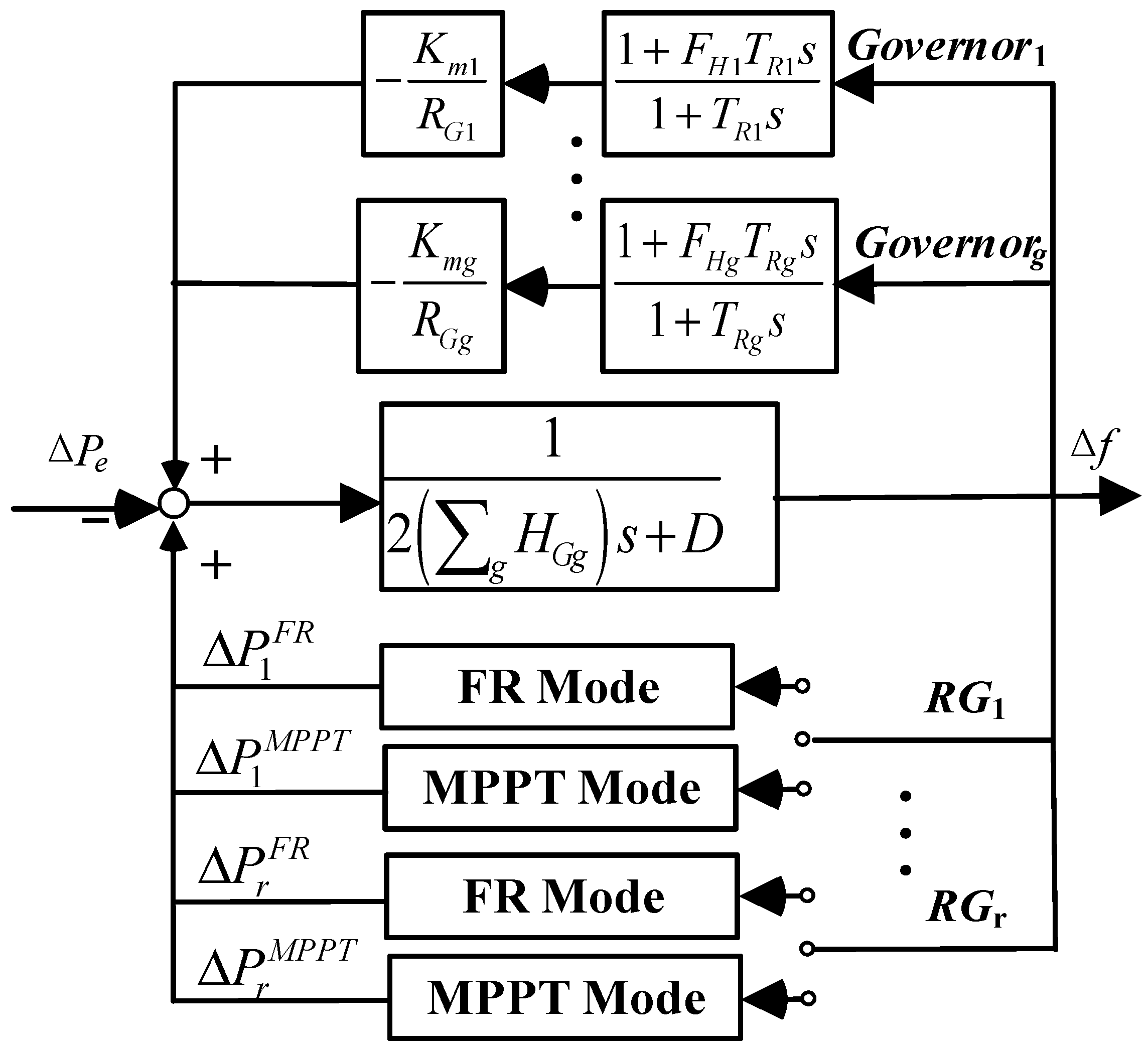
2.1. Frequency Dynamics Modeling

In this section, the control mode transition of RGs is first introduced in Section 2.1.1, and the frequency dynamics are modeled while considering the control mode transition of RGs in Section 2.1.2. Lastly, dynamic frequency models are transformed into the linear algebraic formulation through a ZOH discretization technique in Section 2.1.3.

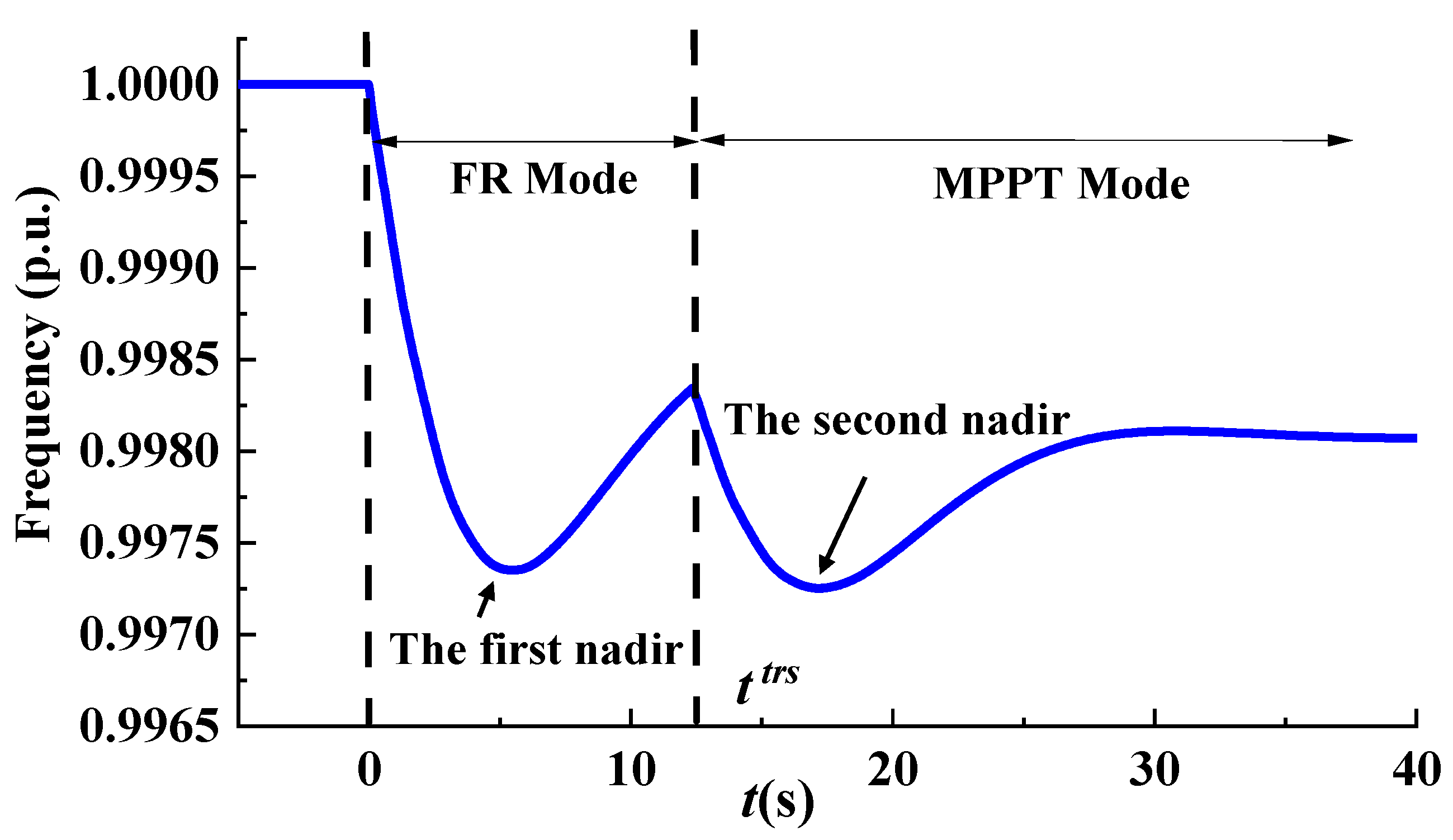
2.1.1. Control Mode Transition of RGs

RGs can respond to the frequency drop by the additional control architecture for the frequency regulation, such as RoCoF loop and droop loop [2]. In this case, RGs can provide more output power than that in MPPT mode to support the system frequency by releasing the stored energy, such as the kinetic energy stored in rotating masses for wind turbines. Considering the RoCoF loop and droop loop for RGs, the increment of the RG output during the FR mode can be modeled as Equation (1).
Δ P r F R = 2 H r v i r t d Δ f d t 1 R r v i r t Δ f , r W
where Δ P r F R is the power increment of the RG r during the FR mode; H r v i r t is the virtual inertial constant in the ROCOF control loop; Δ f is the deviation of the frequency; R r v i r t is the virtual regulation coefficients, and its inverse serves as the gain in the droop control loop; and W is the set of the RG farm.
Subsequently, the control strategy of RGs needs to transmit from the FR mode to the MPPT mode to restore the energy consumed during the frequency support, thereby ensuring the stability of RG units [23]. Taking WTs as an example, the increment of the RG outputs under the MPPT mode can be modeled as Equation (2).
Δ P r M P P T = k r o p t w r 3 k r o p t w r , 0 3 , r W
where Δ P r M P P T is the power increment of the RG r during the MPPT mode; k r o p t is the coefficient of MPPT curve of the WT r; w r and w r , 0 are the rotor electrical angular speed and initial rotor electrical angular speed of WT r, respectively. It is noted that the rotor speed of WTs is relevant with the electrical power outputs P r e , W T and the mechanical power P r m , W T captured from the wind energy, as shown in Equation (3). Moreover, the mechanical power P r m , W T can be modeled as the function of rotor speed, as shown in Equation (4).
2 H r W T w r d w r d t = P r m , W T P r e , W T , r W
P r m , W T = 1 2 ρ q i r π ( R r W T ) 2 C r p ( λ r w , β r ) v r 3 C r p ( λ r w , β r ) = 0.22 116 λ r w 0.8 β r 5 e 12.5 λ r w 1 λ r w = 1 λ r w + 0.08 β r 0.035 β r 3 λ r w = R r W T w r / v r , r W
where H r W T is the inertial constant of the WT r; ρ q i r is the air density; R r W T is the rotor blade radius of the WT r; and β r is the pitch angle of the WT r.
Hence, the increment of the RG output can be modeled as Equation (5) considering the control mode transition, where t t r s is the termination time of the FR mode.
Δ P r e , W T = 2 H r v i r t d Δ f d t 1 R r v i r t Δ f , f o r   t t t r s k r o p t w r 3 k r o p t w r , 0 3               , f o r   t > t t r s , r W

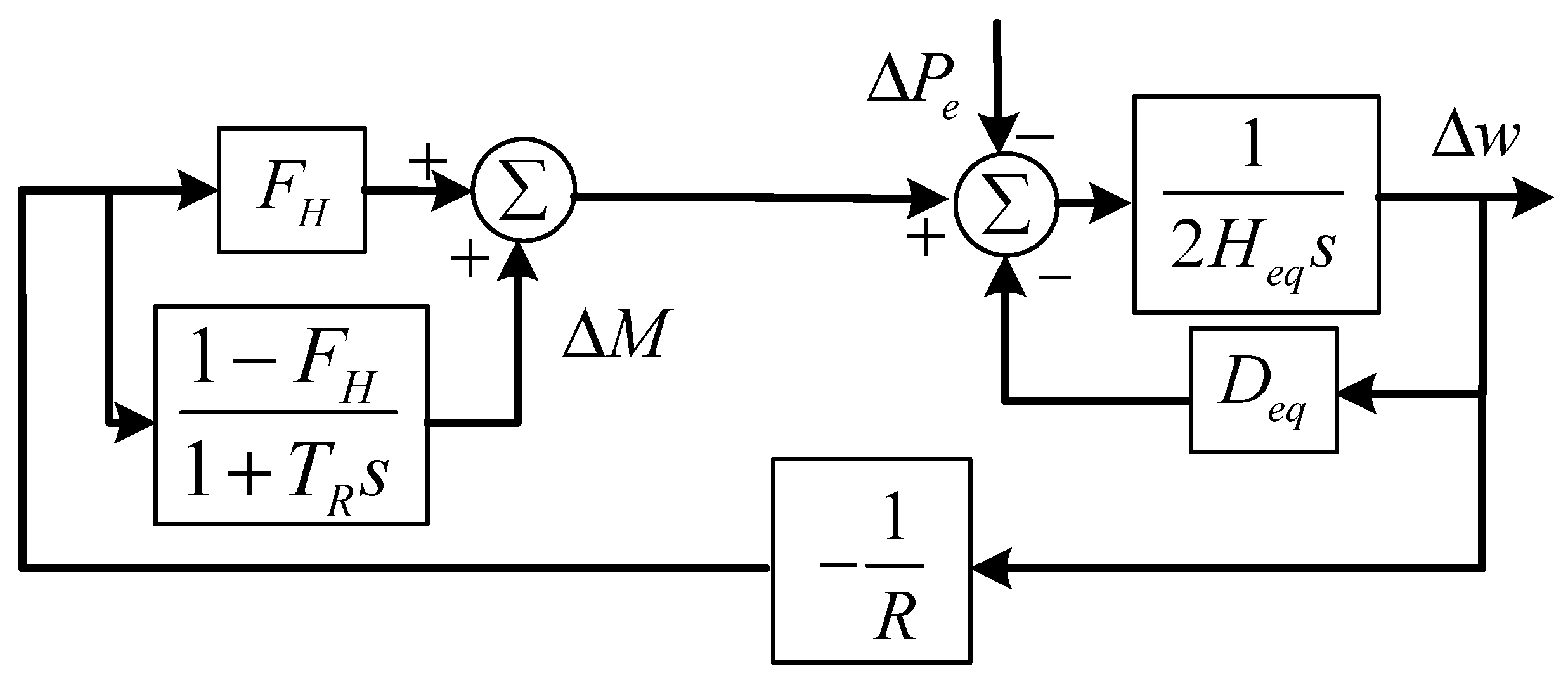
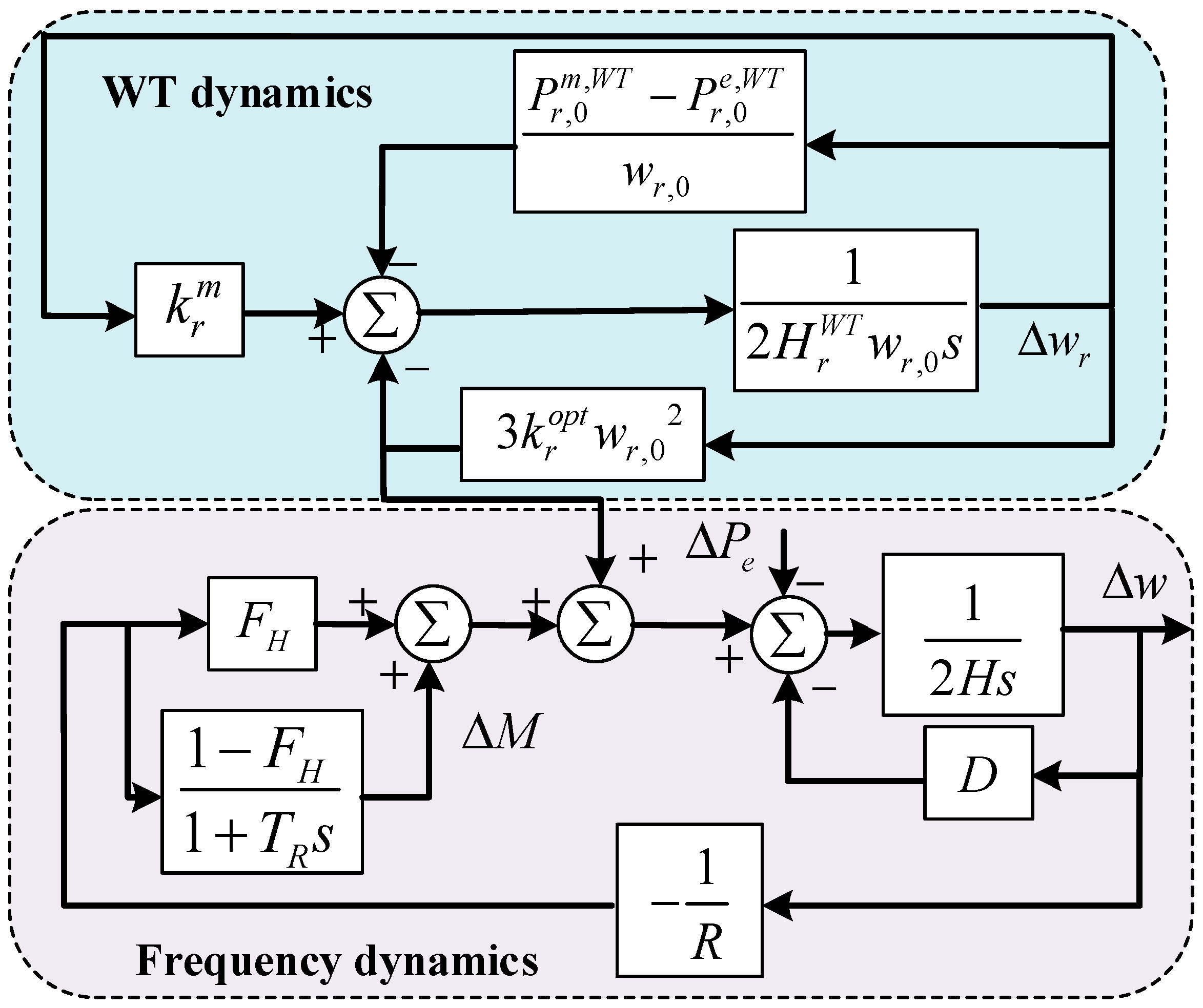
2.1.2. Frequency Dynamic Modeling

Preceding the frequency dynamic modeling, some necessary assumptions for the model development are introduced as follows.
(1)
A low-order frequency response model, which is derived from the multi-machine frequency response model, is adopted in this paper, and the effectiveness of this model has been validated in existing studies [26,27,28,29,30].
(2)
The nonlinear dynamic model of WTs will be linearized through Taylor series to generate a linear time-invariant prediction model in the following text.
(3)
The frequency response of other components, such as loads and storages, are not considered in this paper. However, these frequency response models can be conveniently integrated into the system frequency model under the proposed analysis structure.
First, the frequency dynamics considering the control mode transition of RGs can be characterized as shown in Figure 1, where H G g e and D are the inertia constant and damping constant of the synchronous generation g, respectively; and other parameters concerning the governor response of SGs, such as R G g , K m g , F H g and T G g , can be found in [25].
Next, the multi-governor response model can be aggregated into a single-governor model to reduce the model dimensionality [32]. Specifically, the equivalent parameter of H, R, and FH can be obtained by Equation (6), where S G g and S V w are the rated power of the SG g and RG w, respectively. Then, the aggregated single-machine model can be generated as shown in Figure 2.
H = g H G g S G g / g S G g 1 R = g K m g R G g S G g / g S G g F H = g K m g R G g F H g S G g / 1 R / g S G g
According to the low-order frequency response model, the frequency dynamics can be characterized by the transfer function (7) integrated with the RG output model (5) [25].
Δ f = R ω n 2 D R + 1 1 + T R s s 2 + 2 ς ω n + ω n 2 ( Δ P e + r Δ P r e , W T )
where
ω n 2 = D R + 1 2 H R T R
ς = 2 H R + ( D R + F H ) T R 2 ( D R + 1 ) ω n
where R, D, H, F H , and T R are aggregated governor regulation, damping factor, inertia constant, fraction of total power generated by the turbine and reheat time constant, respectively; Δ P e is the incremental power disturbance; ς and ω n are the damping radio and undamped oscillation frequency of standard 2nd control system, respectively.
It can be seen from Equations (5) and (7) that the system frequency curve is a continuous but nondifferentiable function in the time domain, and this characteristic is attributed to the step-change of Δ P r e , W T at the mode transition time t t r s . A typical multi-segment frequency curve considering the control mode transition of RGs is illustrated in Figure 3. In this case, the derivation of frequency dynamics is extremely challengeable, and its analytical expression is incompatible with the scheduling model due to the nonconvex and nondifferentiable characteristics.

2.1.3. Model Discretization

In this section, dynamic frequency models are transformed into the linear algebraic formulation through a ZOH discretization technique. During the FR mode ( t 0 ~ t t r s ), RGs provide the additional power outputs to support the system frequency, and the details are shown in Equation (1). Hence, the predictive model of the system frequency during the FR mode can be derived from the low-order frequency response model in Figure 4. Moreover, the mathematical formulation of the discretization prediction model is derived from Figure 4, as shown in Equations (10) and (11), and the derivation procedure is provided in the Appendix A.
Δ x F R ( k + 1 ) = A F R Δ x F R ( k ) + B F R Δ u F R ( k ) , k k t r s
Δ y F R ( k ) = C F R Δ x F R ( k ) , k k t r s
where
Δ x F R ( k ) = Δ ω t ( k ) , Δ M t ( k ) , Δ u F R ( k ) = Δ P e , Δ y F R ( k ) = Δ ω t ( k )
A F R = 1 F H + R D e q Δ t 2 H e q R Δ t 2 H e q 1 F H Δ t T R R 1 Δ t T R B F R = Δ t 2 H e q 0 T , C F R = 1 0
H e q = g H G g S G g + r H r v i r t S W r / g S G g + r S W r
D e q = g D G g S G g + r 1 R r v i r t S W r / g S G g + r S W r
where H e q and D e q are the aggregated system inertia and damping factor with the participation of WTs, respectively; Δ x F R , Δ u F R , and Δ y F R are vectors of the state variables, input variables and output variables in the FR mode, respectively; and A F R , B F R and C F R are coefficient matrix of the discretization prediction model in the FR mode.
Then, once the FR mode is terminated at the time t t r s , the MPPT mode will be activated, and the power outputs of RG can be calculated through Equation (2). In this case, the predictive model of the system frequency during the MPPT mode can be derived from the model in Figure 5. Moreover, the mathematical formulation of the discretization prediction model is built in Equations (16) and (17), and the derivation procedure is provided in the Appendix B.
Δ x M P T ( k + 1 ) = A M P T Δ x M P T ( k ) + B M P T Δ u M P T ( k ) , k k t r s
Δ y M P T ( k ) = C M P T Δ x M P T ( k ) , k k t r s
where
Δ x M P T ( k ) = Δ ω t ( k ) , Δ M t ( k ) , Δ w r , t ( k ) , Δ u M P T ( k ) = Δ P e , Δ y M P T ( k ) = Δ ω t ( k )
A M P T = 1 F H + R D Δ t 2 H R Δ t 2 H 3 k r o p t w r , 0 2 Δ t 2 H 1 F H Δ t 2 T R R 1 Δ t T R 0 0 0 1 α r 2 H r W T w r , 0 2
α r = 3 k r o p t w r , 0 3 Δ t P r , 0 m , W T P r , 0 e , W T Δ t + k r m w r , 0 Δ t
k r m = 0.11 ρ q i r π R r W T v r 4 w r , 0 2 188.5 1450 v r R r W T w r , 0 e 12.5 v r R r W T w r , 0
B M P T = Δ t 2 H 0 0 T , C M P T = 1 0 0
where w r , 0 , P r , 0 m , W T , and P r , 0 e , W T are the rotor speed, mechanical and electrical power of WTs at the time t t r s , respectively. The value of w r , 0 can be calculated via the rotor movement equation during the FR mode, and the value of P r , 0 e , W T and P r , 0 m , W T can be obtained through Equations (2) and (4) with the known w r , 0 , respectively; α r , k r m ,   and k r o p t are supplementary variables; Δ x M P T , Δ u M P T ,   and Δ y M P T are vectors of the state variables, input variables and output variables in the MPPT mode, respectively; and A M P T , B M P T ,   and C M P T are coefficient matrix of the discretization prediction model in the FR mode.

2.2. Unit Commitment Model

The predictive model of the system frequency is integrated into the traditional UC model to guarantee the frequency stability in this section. Specifically, the FSCUC model consists of the objective function (23), power balance constraints (24), power output constraints (25) and (26), startup and shutdown constraints (27) and (28), ramping constraints (30) and frequency dynamic constraints (31).

2.2.1. Objective Function

The objective function of the FSCUC model is to minimize the expectation of the operational costs, including the generation cost Fg, unit startup and shutdown cost Fsw and the penalty cost for the wind shedding Fcut, as modeled in Equation (23).
min F = F g + F s w + F c u t F g = s = 1 S t = 1 24 i = 1 N G ρ s C i P s , i , t g F s w = t = 1 24 i = 1 N G ( s t u i , t C o n , i + s h d i , t C o f f , i ) F c u t = s = 1 S t = 1 24 j = 1 N W ρ s C c u t P s , j , max w P s , j , t w )
where NG, NW, and S are the number of the synchronous generators (SGs), wind farms, and operational scenarios, respectively. Ci is the incremental generation cost of the unit i; ρ s is the occurrence probability of the scenario s; P s , i , t g is the active power outputs of the unit i at time t and scenario s; U s , i , t g is the binary variable indicating the on-off states of the unit i at time t and scenario s; Con,i and Coff,i are the startup and shutdown cost of the unit i; s t u i , t and s h d i , t are binary variables indicating the startup and shutdown states of the unit i at time t, respectively; Ccut is the incremental cost of the penalty for the wind shedding; P s , j , m a x w is the forecasting value of the active power of the wind farm j at the scenario s; and P s , j , t w is the active power outputs of the wind farm j at time t and scenario s.

2.2.2. Power Balance Constraints

The power balance between the sources and loads needs to be met, and the DC power flow model is adopted in this paper as shown in Equation (24).
i I ( n ) P s , i , t g + j J ( n ) P s , j , t w + m N ( n ) P s , m n , t = l L ( n ) P s , l , t d , s , t , n P s , m n , t = θ s , m , t θ s , n , t x s , m n , s , t , m n P m n max P s , m n , t P m n max , s , t , m n
where P s , l , t d is the active power of the load l at time t and scenario s; I ( n ) ,   J ( n ) , and L ( n ) are the set of the SG, wind farm, and load at the bus n, respectively; N ( n ) is the set of the bus connecting the bus n; θ s , m , t is the phase angle of the bus m at time t and scenario s; P s , m n , t is the power flow through the line mn at time t and scenario s; x s , m n is the reactance of the line mn; and P m n m a x is the transmission capacity of the line mn.

2.2.3. Power Output Constraints

The power outputs of SGs and wind farms are bounded within the power capacity and the forecasted power, as modeled in (25) and (26), respectively.
U i , t g P i , min g P s , i , t g U i , t g P i , max g , s , t , i
0 P s , j , t w P s , j , max w , s , t , j
where U s , i , t g is the binary variable indicating the on-off states of the unit i at time t and scenario s; and P i , m i n g and P i , m a x g are the minimum and maximum power of the unit i, respectively.

2.2.4. Startup and Shutdown Constraints

The startup and shutdown states are relevant with the on-off state as modeled in (27), and the online and offline time are limited by (28).
U i , t 1 g + U i , t g s t u i , t 0 U i , t 1 g U i , t g s h d i , t 0 , t , i
( X i , t 1 s t T i s t ) ( U i , t 1 g U i , t g ) 0 ( X i , t 1 s h T i s h ) ( U i , t g U i , t 1 g ) 0 , t , i
where X i , t s t and X i , t s h are the continuous online and offline time of the unit i at time t, respectively; and T i s t and T i s h are minimum online and offline time, respectively.
It is noted that the constraints on the minimum online and offline time (28) are nonlinear, which need to be linearized to improve compatibility with the UC model. Taking the minimum online time constraints as the example, the linear formulation is provided in (29).
t = 1 J i 1 U i , t g = 0 , J i = min T , ( T i s t T i , t 0 o n ) U i , t 0 g δ = t t + T i s t 1 U i , δ g T i s t ( U i , t g U i , t 1 g ) , t = J i + 1 , , T T i s t + 1 δ = t T U i , δ g U i , t g U i , t 1 g 0 , t = T T i s t + 2 , , T
where J i is the required time online of the unit i after the initial time; T i , t 0 o n is the time online of the unit i before the initial time; U i , t 0 g is the on-off state of the unit i at the initial time.

2.2.5. Ramping Constraints

The ramping-up and -down power of SGs are limited within required scopes as modeled in Equation (30), where R U i g and R D i g are upper bounds of the ramping-up and -down power of the unit i.
P s , i , t g P s , i , t 1 g U i , t 1 g R U i g + ( U i , t g U i , t 1 g ) P i , min g + ( 1 U i , t g ) P i , max g P s , i , t 1 g P s , i , t g U i , t g R D i g + ( U i , t 1 g U i , t g ) P i , min g + ( 1 U i , t 1 g ) P i , max g , s , t , i

2.2.6. Frequency Dynamic Constraints

The predictive model (10)–(22) can be integrated into the UC model to capture the frequency behaviors. Further, the frequency stability indices are required to guarantee the frequency stability, including the limits on the steady frequency deviation, rate of change in frequency (RoCoF) and the frequency nadir, respectively. These frequency stability indices can be represented using the frequency behaviors in the predictive model, as shown in Equation (31).
R o C o F Δ f s , k + 1 Δ f s , k Δ t R o C o F max Δ f n a d i r Δ f s , k Δ f s , max Δ f s s s Δ f s , K Δ f s , max s s
where Δ f s s is the deviation of the steady frequency; RoCoF is the rate of change in frequency; Δ f n a d i r is the deviation of the frequency nadir; and Δ f m a x s s , R o C o F m a x and Δ f m a x are the upper limits of these frequency indices, respectively.
It is noted that the realizations of the uncertainties concerning the wind power and loads can be generated with the mature sampling and scenario-reduction method, such as the Latin hypercube sampling method and synchronous backpropagation reduction method in [33]. The sampling method is no longer introduced in detail since it is not the main contribution of this paper.
It can be seen that the proposed FSCUC model is a mixed-integer high-dimensional linear problem due to the large quantities of the constraints caused by the frequency predictive model, which poses a considerable challenge to the solution. For this purpose, a PII-based solution algorithm is designed, and the details will be provided in this next section.

3. Solution Method

In this section, a PII-based solution algorithm is designed to decouple the UC model and the frequency stability model, thereby reducing the computational burden significantly. Specifically, the traditional UC model is solved to obtain a cost-optimal solution. Subsequently, the frequency stability of the cost-optimal solution is checked for all scheduling periods, and the inertia for the frequency-instability periods is required to be improved in the UC model. Hence, the high-dimensional FSCUC model can be decomposed, and the computational burden can be reduced. The FSCUC model can be abbreviated as (32) for clear clarification, and the details of the PII-based solution algorithm are provided in Algorithm 1.
min F = F g + F s w + F c u t s . t .   U C   m o d e l :   E q u a t i o n s   ( 24 ) ( 30 )               F r e q u e n c y :   E q u a t i o n s   ( 10 ) , ( 11 ) , ( 16 ) , ( 17 )   a n d   ( 31 )
min F = F g + F s w + F c u t s . t .   U C :   E q u a t i o n s   ( 24 ) ( 30 )               F r e q u e n c y : H t > H k , t c o n s , t φ k
min I k , t s . t .   E q u a t i o n s   ( 10 ) , ( 11 ) , ( 16 ) , ( 17 )   a n d   ( 31 ) , t
Algorithm 1: PII-based solution algorithm
Initialization:
       Set the iterative index k 0
       Set the frequency-instability periods φ k .
Repeat:
            1. Solve UC problem
                Solve UC problem (33) and obtain the cost-optimal UC solution x k * .
            2. Check the Frequency Stability
                         Check the frequency stability through the model (34) using x k * ;
                         Obtain frequency stability index I k , t * and system inertia H k , t c o n s .
            3. Check Convergence Condition
                         If I k , t * > I m a x :
                     set t φ k ;
                                  k k + 1;
                                  Go to Step 1.
                         Else:
                                  Terminate the algorithm.
It can be seen that a low-dimensional UC model (32) and a linear frequency check model (33) are generated through the proposed PII-based solution algorithm, which can ensure the efficient solution with the commercial software, such as the GAMS 23.7/CPLEX 12.3. Moreover, the frequency check model (33) is a time-decoupled problem, whose computational efficiency can be further improved.

4. Case Studies

In this section, case studies are conducted on the modified IEEE 24-Bus and 118-Bus transmission systems. All simulations are performed using the GAMS 23.7/CPLEX 12.3 platform on a computer equipped with a Core i5 3.2 GHz processor and 4 GB RAM.

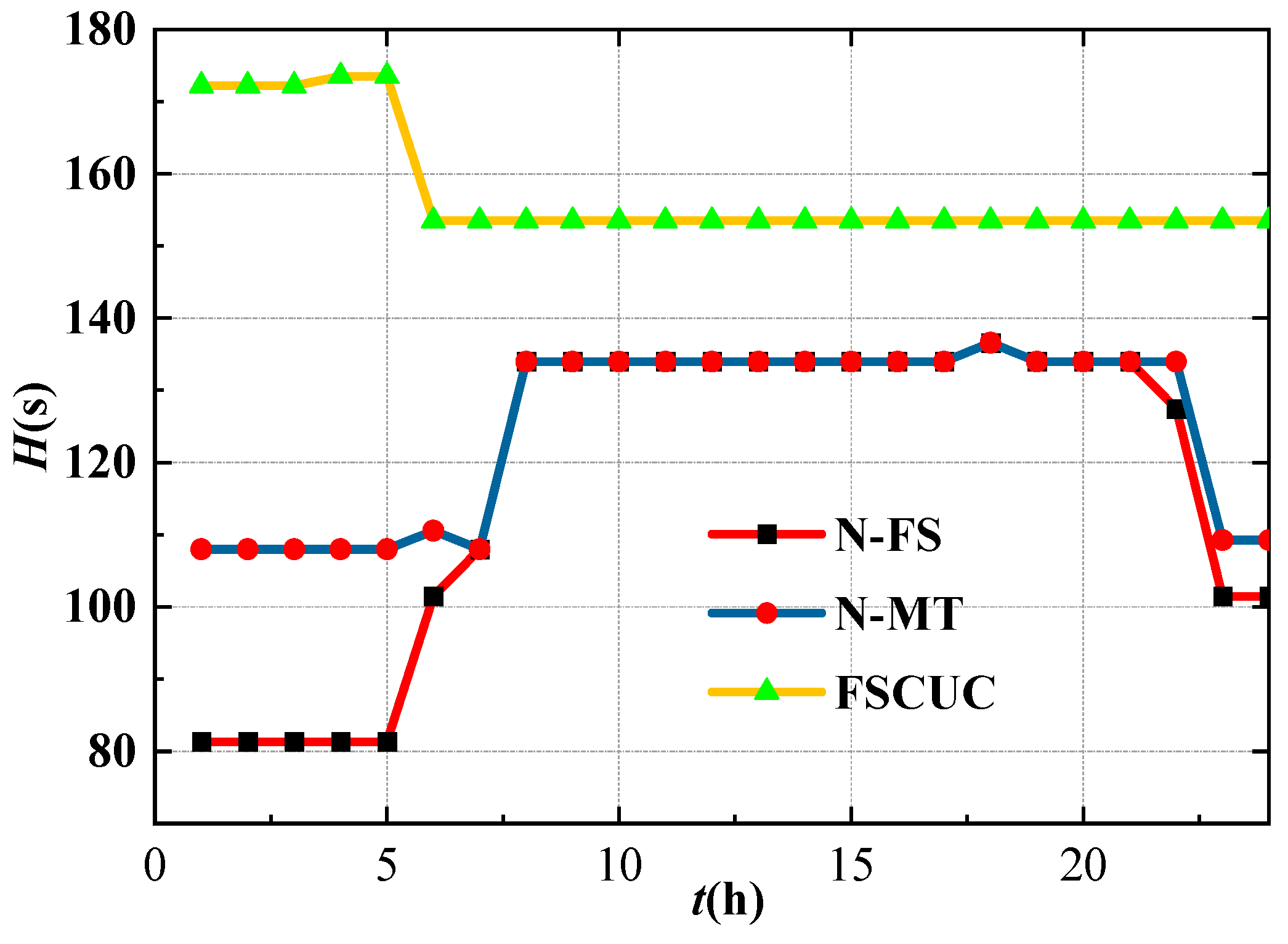
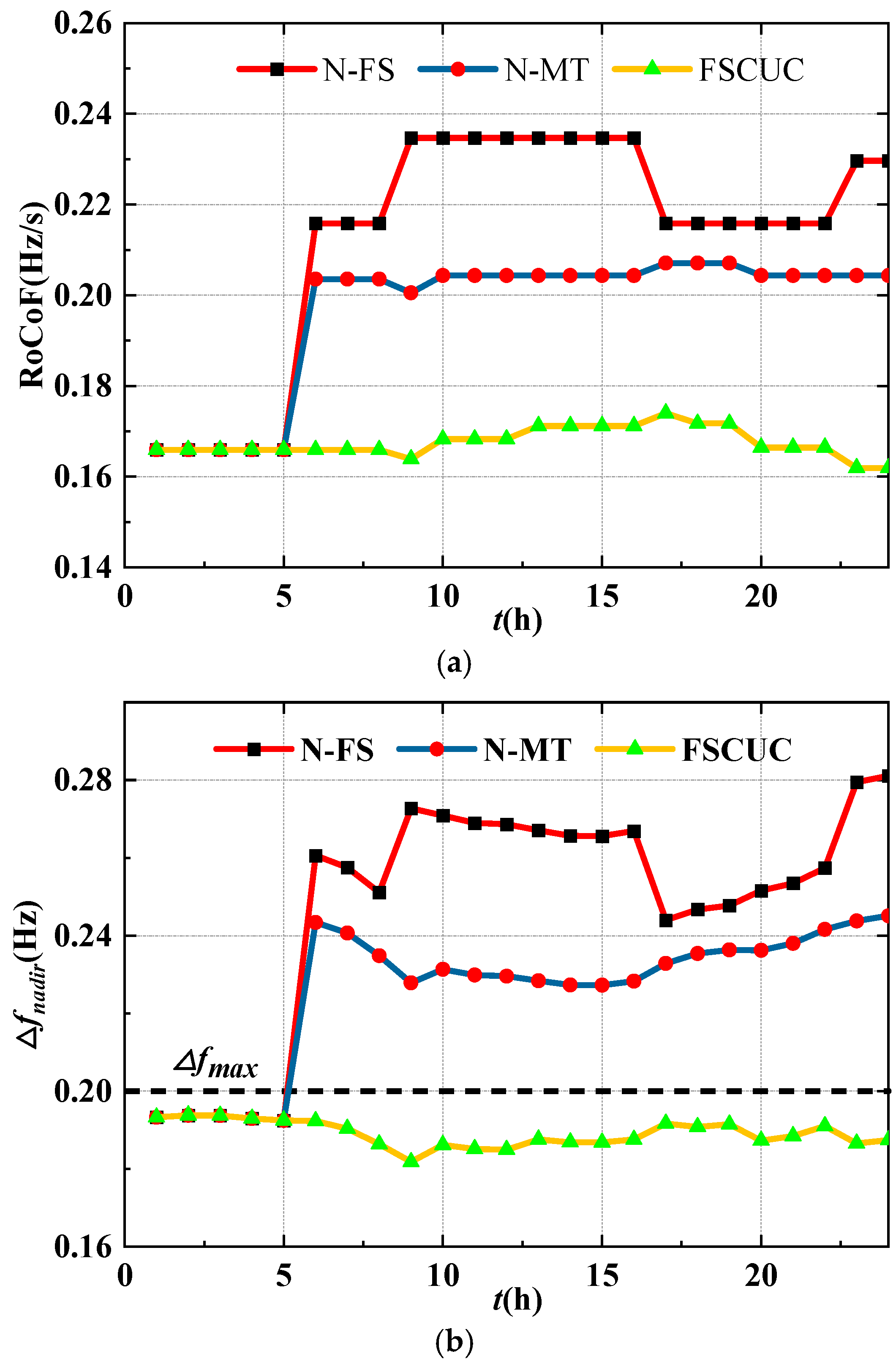
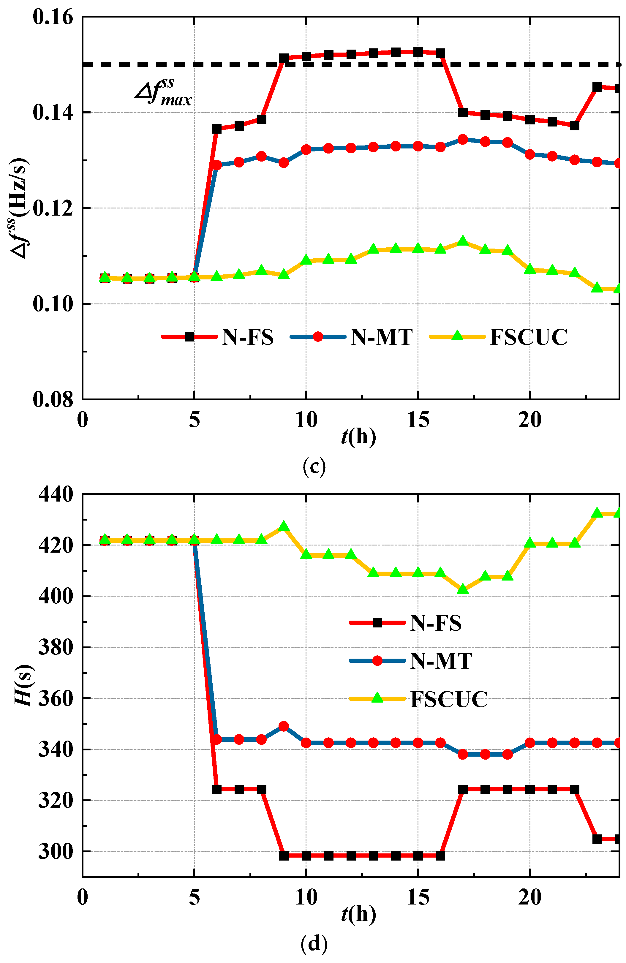
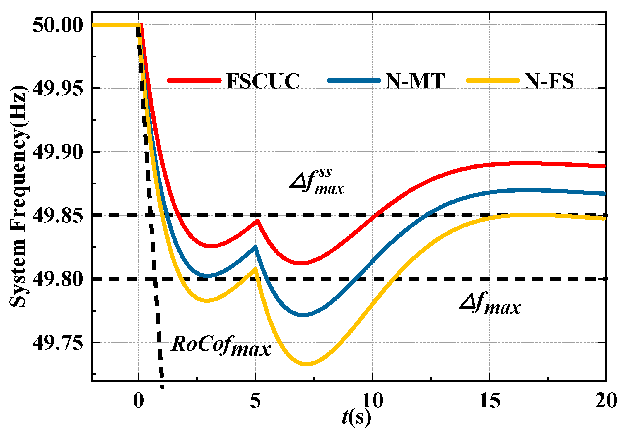
4.1. IEEE 24-Bus System

Case studies are first performed on the modified IEEE 24-Bus system to validate the effectiveness and superiority of the proposed method. Two wind farms are connected to buses 18 and 22, respectively, and each with a capacity of 200 MW. H r v i r t = 5 , R r v i r t = 0.05 , and t t r s = 5   s . It is assumed that the parameters concerning the frequency regulation of WTs have been determined by proper frequency regulation strategies [2,3,4], and the effectiveness of these parameters has been validated in existing frequency-constrained UC models [26,27,28,29,30]. The thresholds of frequency indices are set as R o C o F m a x = 0.2   H z / s , Δ f m a x = 0.2   H z ,   Δ f m a x s s = 0.15   H z . It is noted that the thresholds of frequency indices are determined to avoid the activation of the under-frequency load shedding (UFLS) scheme and the protection mechanisms that are designed to respond to frequency deviation thresholds [26,27,28,29,30]. The sampling time Δt is set as 0.1 s, and the influence of the sampling time will be studied in this section. The prediction horizon is set as 20 s, which ensures that the frequency is in a steady state. By applying the proposed model, the frequency indices and inertia are shown in Table 1, which validates the effectiveness to ensure the frequency stability.
Moreover, the frequency dynamics and WT power output are provided in Figure 6 and Figure 7, respectively, to clarify the control mode transition. During the FR mode (0~5 s), WTs increase the power output through the ROCOF loop and droop loop in Equation (1) to alleviate the frequency drop. Subsequently, the FR mode is terminated, and the MPPT mode is activated at t t r s = 5   s to ensure the stability of WTs and restore the rotor speed. In this case, the power outputs of WTs decline significantly, causing the severe second frequency, reaching to the Δ f m a x = 0.2   H z , as shown in Figure 6. Therefore, the necessity to involve the control mode transition into the UC model is highlighted, and the effectiveness of the proposed can be validated.
Moreover, the influence of the sampling time on the precision and computational time is studied. The simulation results are shown in Table 2, where T ( 34 ) is the computational time for solving the model (34). It can be seen that a larger sampling time leads to a greater relative error, which can reach 4.9% when Δt = 0.4 s. Moreover, a larger sampling time can decrease computation time by reducing the model dimensionality. However, the increase in the computation time is acceptable for these sampling cases due to the linearity of the model (34). Hence, the numerical simulations should be performed to determine the sampling time before the UC model implementation, so that the model accuracy can be guaranteed. In this case study, the sampling time of 0.1 s is precise enough for the UC model, which is adopted in this paper.
Subsequently, the proposed FSCUC model is compared with the existing method to validate the superiority, including the traditional UC model without frequency constraints (N-FS) [9] and without control mode transition (N-MT) [22]. The comparison of operational costs and frequency indices are shown in Table 3 and Figure 8, and the improvement of frequency indices and inertia compared to the N-FS model is provided in Table 4. It can be seen that the limits on the frequency indices are violated in the N-FS model, and limits on RoCoF and frequency nadirs are not guaranteed in the N-MT model. In contrast, limits on all frequency indices can be strictly met in the proposed FSCUC model with the additional costs of only 0.66%. Moreover, frequency indices and inertia can be improved by 53%, 59%, 52%, and 113% at most, respectively, as shown in Table 4. Hence, the superiority of the proposed method to address the frequency stability can be demonstrated.
In addition, the frequency dynamics and WT power are compared among N-FS, N-MT, and FSCUC models, as shown in Figure 9 and Figure 10. It can be seen that both the first and second nadirs are lower than the limits in the N-FS model. In the N-MT model, the first nadir is considered in the UC model, which ensures the frequency security during the FR mode, but causes the severe frequency drop during the MPPT mode. For this reason, WTs provide too much power output during the FR mode, leading to the severe drop of rotor speed and the power drop at the mode transition time, as shown in Figure 10. In comparison, sufficient inertia is ensured in the proposed method in Figure 11, which improves the first and second nadir simultaneously of 47%.

4.2. IEEE 118-Bus System

Numerical tests are further performed on the modified IEEE 24-Bus system to validate the effectiveness and superiority for larger systems. Three wind farms are connected to the bus 36, 69, and 77, respectively, and each with a capacity of 200 MW. Other parameters are identical with these in the 24-Bus system. The proposed FSCUC model is compared with the N-FS and N-MT model, and the comparison results are shown in Table 5 and Figure 12. Moreover, the improvement of frequency indices and inertia compared to the N-FS model is provided in Table 6. It can be seen that the frequency indices and inertia can be improved by 30%, 33%, 30%, and 43% at most, respectively. Hence, frequency stability during the FR and MPPT mode can be strictly guaranteed by improving the system inertia, and only 3.1% of the operational costs are increased. Moreover, the frequency dynamics are compared among N-FS, N-MT, and FSCUC models, and the comparison results are shown in Figure 13, which indicates the necessity to consider the control mode transition in the UC model, and the effectiveness of the proposed method.
The effectiveness of the PII-based solution algorithm is demonstrated, and the convergence behaviors and the evolution of the frequency–instability periods are shown in Figure 14 and Table 7, respectively. Moreover, a comparison of the computation time between the proposed and direct solution method is shown in Table 8. It can be seen that the proposed method can converge within six iterations, spending 5 min, and both the frequency index and frequency–instability periods can be reduced effectively. In contrast, the direct solution method is unable to converge to a feasible solution within 10 h due to the high-dimensional characteristic of the FSCUC model.

5. Discussion

To satisfy the inertia requirements, a novel FSCUC model is proposed while considering control mode transition of renewable generations. The dynamic frequency behaviors considering the control mode transition are modeled through the ZOH discretization technique, and the frequency predictive model is integrated into a stochastic UC model. Moreover, a PII-based solution algorithm is proposed to improve computational efficiency. The numerical tests demonstrate the necessity to consider the mode transition in the UC model. The proposed method can ensure frequency stability during both FR and MPPT modes with the negligible increase in operational costs when compared with other existing methods. The PII-based solution algorithm can converge to a high-quality solution within several iterations, which reduces the computational burden significantly. Consequently, the effectiveness and the superiority of the proposed method can be validated.
In this paper, the frequency dynamic is modeled with the low-order frequency response model, which ignores the spatial characteristic of the system frequency. Moreover, the fluctuation of wind speed and the frequency regulation of loads also play an essential role in frequency stability, which remains to be addressed in the future research. In addition, overcurrent due to excessive short-circuit current is a critical challenge in the scheduling of renewable-dominated power systems, which will also be addressed in future studies.

Author Contributions

Conceptualization, F.Y., L.G. and S.W.; Methodology, F.Y., L.G. and S.W.; Software, F.Y., L.G. and S.W.; Validation, F.Y., L.G. and S.W.; Formal analysis, F.Y. and S.W.; Investigation, F.Y. and S.W.; Resources, F.Y. and S.W.; Data curation, F.Y., L.G. and S.W.; Writing—original draft, F.Y., L.G. and S.W.; Writing—review and editing, F.Y., L.G. and S.W. All authors have read and agreed to the published version of the manuscript.

Funding

This research was funded by State Grid Science & Technology Project in China, grant number 4000-202316071A-1-1-ZN.

Data Availability Statement

Data is contained within the article.

Conflicts of Interest

The authors declare that this research was conducted in the absence of any commercial or financial relationships that could be construed as a potential conflict of interest. The authors declare that this study received funding from the State Grid Science & Technology Project in China, grant number 4000-202316071A-1-1-ZN. The funders had no role in the design of this study; in the collection, analyses, or interpretation of data; in the writing of the manuscript; or in the decision to publish the results.

Abbreviations

The following abbreviations are used in this manuscript:
FRFrequency regulation
FSCUCFrequency stability constrained unit commitment
MPPTMaximum power point tracking
PIIProgressive inertia increment
RGRenewable generation
SGSynchronous generation
UCUnit commitment
WTWind turbine
ZOHZero-Order Hold

Appendix A

According Figure 4, the state–space expression can be first obtained as shown in Equation (A1) by assigning Δ ω and Δ M as the state variables.
d Δ ω d t d Δ M d t = F H + R D e q 2 H e q R 1 2 H e q 1 F H T R R 1 T R Δ ω Δ M + 1 2 H e q 0 Δ P e
Subsequently, the differential terms are discretized through a ZOH discretization technique, so that Equation (A1) can be reformulated as Equation (A2).
Δ ω t ( k + 1 ) Δ ω t ( k ) Δ t Δ M t ( k + 1 ) Δ M t ( k ) Δ t = F H + R D e q 2 H e q R 1 2 H e q 1 F H T R R 1 T R Δ ω t ( k ) Δ M t ( k ) + 1 2 H e q 0 Δ P e
Last, the discretization prediction model in the FR model can be obtained from (A2) by assigning Δ ω as the output, i.e., Equations (10) and (11).

Appendix B

A linear time-invariant prediction model can improve the solvability of the UC model. Hence, the electrical and mechanical power of WTs in (2) and (4) should be linearized to be compatible with the ZOH discretization technique and the FSCUC model. Compared with the piecewise linearization method, the Taylor expansion method can linearize Equations (2) and (4) without binary variables by retaining the first-order term, as shown in Equations (A3) and (A4), respectively.
Δ P r M P P T = 3 k r o p t w r , 0 2 Δ w r , r W
Δ P r m , W T = d P r m , W T d w r w r = w r , 0 Δ w r = k r m Δ w r
Then, the rotor movement equation of WTs (3) is reformulated as Equation (A5) by integrating (3) and (A6).
2 H r W T w r , 0 d Δ w r d t = Δ P r m , W T Δ P r e , W T P r , 0 m , W T P r , 0 e , W T w r , 0 Δ w r
w r = w r , 0 + Δ w r P r m , W T = P r , 0 m , W T + Δ P r m , W T P r e , W T = P r , 0 e , W T + Δ P r e , W T
Subsequently, Equation (A7) can be obtained by combining (A3), (A4), and (A5).
d Δ w r d t = k r m w r , 0 3 k r o p t w r , 0 3 P r , 0 m , W T P r , 0 e , W T 2 H r W T w r , 0 2 Δ w r
In addition, according Figure 5 and Equation (A7), the state–space expression can be first obtained as shown in Equation (A8) by assigning Δ ω , Δ M , and Δ w r as the state variables.
d Δ ω d t d Δ M d t d Δ w r d t = F H + R D e q 2 H e q R 1 2 H 3 k r o p t w r , 0 2 2 H 1 F H T R R 1 T R 0 0 0 α r 2 H r W T w r , 0 2 Δ t Δ ω Δ M Δ w r + 1 2 H e q 0 0 Δ P e
The differential terms in Equation (A8) are discretized through a ZOH discretization technique, so that Equation (A8) can be reformulated as Equation (A9).
Δ ω t ( k + 1 ) Δ ω t ( k ) Δ t Δ M t ( k + 1 ) Δ M t ( k ) Δ t Δ w r , t ( k + 1 ) Δ w r , t ( k ) Δ t = F H + R D e q 2 H e q R 1 2 H 3 k r o p t w r , 0 2 2 H 1 F H T R R 1 T R 0 0 0 α r 2 H r W T w r , 0 2 Δ t Δ ω t ( k ) Δ M t ( k ) Δ w r , t ( k ) + 1 2 H e q 0 0 Δ P e
Finally, the discretization prediction model in the MPPT mode can be obtained from (A9) by assigning Δ ω as the output, i.e., Equations (16) and (17).

References

  1. Kheshti, M.; Ding, L.; Bao, W.; Yin, M.; Wu, Q.; Terzija, V. Toward Intelligent Inertial Frequency Participation of Wind Farms for the Grid Frequency Control. IEEE Trans. Ind. Inform. 2020, 16, 6772–6786. [Google Scholar] [CrossRef]
  2. Morren, J.; Haan, S.W.H.d.; Kling, W.L.; Ferreira, J.A. Wind turbines emulating inertia and supporting primary frequency control. IEEE Trans. Power Syst. 2006, 21, 433–434. [Google Scholar] [CrossRef]
  3. Kou, P.; Liang, D.; Yu, L.; Gao, L. Nonlinear Model Predictive Control of Wind Farm for System Frequency Support. IEEE Trans. Power Syst. 2019, 34, 3547–3561. [Google Scholar] [CrossRef]
  4. Conroy, J.F.; Watson, R. Frequency Response Capability of Full Converter Wind Turbine Generators in Comparison to Conventional Generation. IEEE Trans. Power Syst. 2008, 23, 649–656. [Google Scholar] [CrossRef]
  5. Bao, W.; Wu, Q.; Ding, L.; Huang, S.; Terzija, V. A Hierarchical Inertial Control Scheme for Multiple Wind Farms with BESSs Based on ADMM. IEEE Trans. Sustain. Energy 2021, 12, 751–760. [Google Scholar] [CrossRef]
  6. Xu, Y.; Dong, Z.; Li, Z.; Liu, Y.; Ding, Z. Distributed Optimization for Integrated Frequency Regulation and Economic Dispatch in Microgrids. IEEE Trans. Smart Grid 2021, 12, 4595–4606. [Google Scholar] [CrossRef]
  7. Wang, L.; Yang, Y.; Gu, H.; Zhang, Y.; Wei, C.; Cheng, S. Bottleneck Generator Identification and the Corresponding N-1 Frequency Security Constrained Intraday Generator Dispatch. IEEE Trans. Power Syst. 2023, 38, 739–752. [Google Scholar] [CrossRef]
  8. Alex, N.F.; Gómez, J.S.; Llanos, J.; Rute, E.; Sáez, D.; Sumner, M. Distributed Predictive Control Strategy for Frequency Restoration of Microgrids Considering Optimal Dispatch. IEEE Trans. Smart Grid 2021, 12, 2748–2759. [Google Scholar]
  9. Troxell, D.; Ahn, M.; Gangammanavar, H. A Cardinality Minimization Approach to Security-Constrained Economic Dispatch. IEEE Trans. Power Syst. 2022, 37, 3642–3652. [Google Scholar] [CrossRef]
  10. Ahmadi, A.; Nezhad, A.E.; Hredzak, B. Security-Constrained Unit Commitment in Presence of Lithium-Ion Battery Storage Units Using Information-Gap Decision Theory. IEEE Trans. Ind. Inform. 2019, 15, 148–157. [Google Scholar] [CrossRef]
  11. Li, H.; Zhang, H.; Liu, D.; Zhang, J.; Wong, C.K. Frequency-Constrained Dispatching for an Integrated Electricity-Heat Microgrid With Synergic Regulation Resources. IEEE Trans. Ind. Appl. 2025, 61, 2203–2215. [Google Scholar] [CrossRef]
  12. Qi, X.; Zhao, T.; Liu, X.; Wang, P. Three-Stage Stochastic Unit Commitment for Microgrids Toward Frequency Security via Renewable Energy Deloading. IEEE Trans. Smart Grid 2023, 14, 4256–4267. [Google Scholar] [CrossRef]
  13. Cai, S.; Xie, Y.; Zhang, Y.; Bao, W.; Wu, Q.; Chen, C.; Guo, J. Frequency Constrained Proactive Scheduling for Secure Microgrid Formation in Wind Power Penetrated Distribution Systems. IEEE Trans. Smart Grid 2025, 16, 989–1002. [Google Scholar] [CrossRef]
  14. Yang, L.; Li, H.; Zhang, H.; Wu, Q.; Cao, X. Stochastic-Distributionally Robust Frequency-Constrained Optimal Planning for an Isolated Microgrid. IEEE Trans. Sustain. Energy 2024, 15, 2155–2169. [Google Scholar] [CrossRef]
  15. She, B.; Li, F.; Cui, H.; Wang, J.; Zhang, Q.; Bo, R. Virtual Inertia Scheduling (VIS) for Real-Time Economic Dispatch of IBR-Penetrated Power Systems. IEEE Trans. Sustain. Energy 2024, 15, 938–951. [Google Scholar] [CrossRef]
  16. Wang, C.; Zhang, R.; Bi, T. Energy Management of Distribution-Level Integrated Electric-Gas Systems With Fast Frequency Reserve. IEEE Trans. Power Syst. 2024, 39, 4208–4223. [Google Scholar] [CrossRef]
  17. Cai, S.; Xie, Y.; Zhang, Y.; Zhang, M.; Wu, Q.; Guo, J. A Simulation-Assisted Proactive Scheduling Method for Secure Microgrid Formation Under Static and Transient Islanding Constraints. IEEE Trans. Smart Grid 2024, 15, 272–285. [Google Scholar] [CrossRef]
  18. Javadi, M.; Gong, Y.; Chung, C.Y. Frequency Stability Constrained BESS Sizing Model for Microgrids. IEEE Trans. Power Syst. 2024, 39, 2866–2878. [Google Scholar] [CrossRef]
  19. Zhang, Q.; Ma, Z.; Zhu, Y.; Wang, Z. A Two-Level Simulation-Assisted Sequential Distribution System Restoration Model With Frequency Dynamics Constraints. IEEE Trans. Smart Grid 2021, 12, 3835–3846. [Google Scholar] [CrossRef]
  20. Xu, T.; Jang, W.; Overbye, T. Commitment of Fast-Responding Storage Devices to Mimic Inertia for the Enhancement of Primary Frequency Response. IEEE Trans. Power Syst. 2018, 33, 1219–1230. [Google Scholar] [CrossRef]
  21. Hao, L.; Ji, J.; Xie, D.; Wang, H.; Li, W.; Asaah, P. Scenario-based Unit Commitment Optimization for Power System with Large-scale Wind Power Participating in Primary Frequency Regulation. J. Mod. Power Syst. Clean Energy 2020, 8, 1259–1267. [Google Scholar] [CrossRef]
  22. Javadi, M.; Gong, Y.; Chung, C.Y. Frequency Stability Constrained Microgrid Scheduling Considering Seamless Islanding. IEEE Trans. Power Syst. 2022, 37, 306–316. [Google Scholar] [CrossRef]
  23. Zhang, G.; Zhang, F.; Ding, L.; Meng, K.; Dong, Z.Y. Wind Farm Level Coordination for Optimal Inertial Control with a Second-Order Cone Predictive Model. IEEE Trans. Sustain. Energy 2021, 12, 2353–2366. [Google Scholar] [CrossRef]
  24. Zhao, X.; Wei, H.; Qi, J.; Li, P.; Bai, X. Frequency Stability Constrained Optimal Power Flow Incorporating Differential Algebraic Equations of Governor Dynamics. IEEE Trans. Power Syst. 2021, 36, 1666–1676. [Google Scholar] [CrossRef]
  25. Anderson, P.M.; Mirheydar, M. A low-order system frequency response model. IEEE Trans. Power Syst. 1990, 5, 720–729. [Google Scholar] [CrossRef]
  26. Wen, Y.; Li, W.; Huang, G.; Liu, X. Frequency Dynamics Constrained Unit Commitment With Battery Energy Storage. IEEE Trans. Power Syst. 2016, 31, 5115–5125. [Google Scholar] [CrossRef]
  27. Badesa, L.; Teng, F.; Strbac, G. Simultaneous Scheduling of Multiple Frequency Services in Stochastic Unit Commitment. IEEE Trans. Power Syst. 2019, 34, 3858–3868. [Google Scholar] [CrossRef]
  28. Yang, Y.; Peng, J.C.H.; Ye, C.; Ye, Z.S.; Ding, Y. A Criterion and Stochastic Unit Commitment Towards Frequency Resilience of Power Systems. IEEE Trans. Power Syst. 2022, 37, 640–652. [Google Scholar] [CrossRef]
  29. Zhang, Z.; Du, E.; Teng, F.; Zhang, N.; Kang, C. Modeling Frequency Dynamics in Unit Commitment With a High Share of Renewable Energy. IEEE Trans. Power Syst. 2020, 35, 4383–4395. [Google Scholar] [CrossRef]
  30. Zhang, C.; Liu, L.; Cheng, H.; Liu, D.; Zhang, J.; Li, G. Frequency-constrained Co-planning of Generation and Energy Storage with High-penetration Renewable Energy. J. Mod. Power Syst. Clean Energy 2021, 9, 760–775. [Google Scholar] [CrossRef]
  31. Paturet, M.; Markovic, U.; Delikaraoglou, S.; Vrettos, E.; Aristidou, P.; Hug, G. Stochastic Unit Commitment in Low-Inertia Grids. IEEE Trans. Power Syst. 2020, 35, 3448–3458. [Google Scholar] [CrossRef]
  32. Shi, Q.; Li, F.; Cui, H. Analytical Method to Aggregate Multi-Machine SFR Model with Applications in Power System Dynamic Studies. IEEE Trans. Power Syst. 2018, 33, 6355–6367. [Google Scholar] [CrossRef]
  33. Luo, F.; Bu, Q.; Ye, Z.; Yuan, Y.; Gao, L.; Lv, P. Dynamic Reconstruction Strategy of Distribution Network Based on Uncertainty Modeling and Impact Analysis of Wind and Photovoltaic Power. IEEE Access 2024, 12, 64069–64078. [Google Scholar] [CrossRef]
Figure 1. Multi-machine frequency response model.
Symmetry 17 00752 g001
Figure 2. Low-order frequency response model.
Symmetry 17 00752 g002
Figure 3. A typical multi-segment frequency curve.
Symmetry 17 00752 g003
Figure 4. Frequency response model during FR mode.
Symmetry 17 00752 g004
Figure 5. Frequency response model during MPPT mode.
Symmetry 17 00752 g005
Figure 6. Frequency dynamics of the FSCUC model.
Symmetry 17 00752 g006
Figure 7. WT power output of the FSCUC model.
Symmetry 17 00752 g007
Figure 8. (a) Comparison of the RoCoF with different models. (b) Comparison of the frequency nadir with different models. (c) Comparison of the steady frequency with different models.
Symmetry 17 00752 g008
Figure 9. (a) The comparison of the frequency dynamics at t = 4 h with different models. (b) The comparison of the frequency dynamics at t = 24 h with different models.
Symmetry 17 00752 g009aSymmetry 17 00752 g009b
Figure 10. (a) The comparison of the WT power at t = 4 h with different models. (b) The comparison of the WT power at t = 24 h with different models.
Symmetry 17 00752 g010
Figure 11. The comparison of the system inertia with different models.
Symmetry 17 00752 g011
Figure 12. (a) Comparison of the RoCoF with different models. (b) Comparison of the frequency nadir with different models. (c) Comparison of the steady frequency with different models. (d) The comparison of the system inertia with different models.
Symmetry 17 00752 g012aSymmetry 17 00752 g012b
Figure 13. The comparison of the frequency dynamics with different models.
Symmetry 17 00752 g013
Figure 14. The evolution of the frequency nadir along with the iteration.
Symmetry 17 00752 g014
Table 1. Frequency indices and inertia of the FSCUC model.
Time (h)RoCoF (Hz/s) Δ f n a d i r (Hz) Δ f s s (Hz)H (s)
10.14520.17160.0922172.185
20.14520.17180.0922172.185
30.14520.17260.092172.185
40.14410.17220.0911173.485
50.14410.17360.0909173.485
60.16290.19870.1027153.465
70.16290.19440.1036153.465
80.16290.19050.1044153.465
90.16290.18940.1046153.465
100.16290.18950.1046153.465
110.16290.18860.1048153.465
120.16290.18640.1052153.465
130.16290.18460.1056153.465
140.16290.18370.1058153.465
150.16290.18410.1057153.465
160.16290.18490.1055153.465
170.16290.18550.1054153.465
180.16290.18640.1052153.465
190.16290.18840.1049153.465
200.16290.18990.1045153.465
210.16290.19220.1041153.465
220.16290.19360.1037153.465
230.16290.1950.1035153.465
240.16290.19590.1033153.465
Table 2. Comparison results on Δ f n a d i r and computational time under different sampling times.
Sampling Time Relative   Error   of   Δ f n a d i r (Hz) T ( 34 ) (s)
t = 4 ht = 14 ht = 21 ht = 24 h
0.1 s0.93960.45600.56130.777946
0.2 s2.17601.04191.29411.795439
0.3 s3.49071.11221.62032.693437
0.4 s4.90521.18871.86163.666934
Table 3. Comparison among N-FS, N-MT, and FSCUC model in IEEE 24-Bus system.
Cost ($)MaxRoCoF (Hz/s) m a x Δ f n a d i r (Hz) m a x Δ f s s (Hz)
N-FS1,981,0750.3075 (×)0.4300 (×)0.1920 (×)
N-MT1,982,4750.2316 (×)0.3050 (×)0.1463 (√)
FSCUC1,994,2000.1629 (√)0.1987 (√)0.1058 (√)
(×) and (√) indicate the limits are and are not violated, respectively.
Table 4. Improvement of frequency indices and inertia compared to the N-FS model.
Time (h)RoCoF (%) Δ f n a d i r (%) Δ f s s (%)H (%)
152.7758.9652.02111.75
252.7758.9852.00111.75
352.7759.0551.95111.75
453.1259.5152.23113.35
553.1259.6252.14113.35
633.8938.9333.2051.25
729.6633.9329.2042.14
812.7014.5612.5814.56
912.7014.5212.5914.56
1012.7014.5212.5914.56
1112.7014.4812.614.56
1212.7014.3912.6414.56
1312.7014.3212.6814.56
1412.7014.2812.6814.56
1512.7014.312.6814.56
1612.7014.3312.6714.56
1712.7014.3712.6614.56
1811.0312.4810.9612.38
1912.7014.4812.6114.56
2012.7014.5312.5814.56
2112.7014.6112.5414.56
2216.9319.5116.6920.40
2333.8938.6933.3651.25
2433.8938.7633.3251.25
Table 5. Comparison between N-FS, N-MT, and FSCUC model in IEEE 118-Bus system.
Cost ($)MaxRoCoF (Hz/s) m a x Δ f n a d i r (Hz) m a x Δ f s s (Hz)
N-FS5,367,1000.2346 (×)0.2811 (×)0.1526 (×)
N-MT5,400,0600.2071 (×)0.2451 (×)0.1344 (√)
FSCUC5,539,2350.1740 (√)0.1938 (√)0.1129 (√)
(×) and (√) indicate the limits are and are not violated, respectively.
Table 6. Improvement of frequency indices and inertia compared to the N-FS model.
Time (h)RoCoF (%) Δ f n a d i r (%) Δ f s s (%)H (%)
10000
20000
30000
40000
50000
623.1126.2022.7430.06
723.1126.0722.7930.06
823.1125.7822.9430.06
930.1333.3230.0043.14
1028.2831.2628.1939.43
1128.2831.1628.2239.43
1228.2831.1428.2339.43
1327.0329.7527.0037.04
1427.0329.6627.0237.04
1527.0329.6727.0337.04
1627.0329.7327.0137.04
1719.3921.4319.3524.05
1820.4222.6620.3425.65
1920.4222.7120.3125.65
2022.8825.5522.6929.66
2122.8825.6422.6529.66
2222.8825.8022.5629.66
2329.4733.2329.0241.79
2429.4733.3028.9941.79
Table 7. The evolution of the frequency–instability periods along with the iteration.
123456789101112131415161718192021222324
Iteration 1
Iteration 2
Iteration 3
Iteration 4
Iteration 5
Iteration 6
Symmetry 17 00752 i001 indicates the frequency-instability periods. Symmetry 17 00752 i002 indicates the frequency-stability periods.
Table 8. Comparison of the computation time between the proposed and direct solution method.
Proposed PII-Based MethodDirect Solution
Model (33)Model (34)Total
Time186 s128 s314 s10 h
Disclaimer/Publisher’s Note: The statements, opinions and data contained in all publications are solely those of the individual author(s) and contributor(s) and not of MDPI and/or the editor(s). MDPI and/or the editor(s) disclaim responsibility for any injury to people or property resulting from any ideas, methods, instructions or products referred to in the content.

