Performance Prediction of Store and Forward Telemedicine Using Graph Theoretic Approach of Symmetry Queueing Network

Abstract

In the evolving landscape of healthcare, telemedicine has emerged as a transformative solution, effectively bridging gaps in medical service delivery across diverse geographic regions. Particularly in rural areas, where access to immediate and specialized care remains limited, store-and-forward telemedicine provides a powerful and practical approach. In rural emergency healthcare settings, resource limitations, specialist shortages, and unreliable connectivity frequently delay critical medical interventions. To address these challenges, this study proposes a store-and-forward telemedicine framework optimized through the use of queueing networks, aiming to enhance emergency response efficiency. The proposed model is structured as a four-node system comprising initial registration, consultation, diagnosis, and treatment. Each node operates as a service queue where patient data are sequentially collected, prioritized, and forwarded. By employing an open queueing network structure, the model devises steady-state probabilities for the number of patients at each node, facilitating a detailed performance analysis of patient flows. Symmetry plays a critical role in maintaining patient flow balance and system stability within the store-and-forward telemedicine model. When the routing probabilities between nodes are balanced, the queueing network exhibits probabilistic symmetry, ensuring consistent transition behavior. Moreover, the directed graph representation of the system demonstrates structural symmetry, reflecting identical service times at all nodes and uniform transition probabilities between nodes. Incorporating the concept of symmetry enables a simplified analytical approach, reduces computational complexity, and provides a more accurate approximation model for evaluating system performance.

1. Introduction

When entities that require services—commonly referred to as “customers”—arrive at a service facility and are immediately served, queues or waiting lines are formed. In the context of healthcare, rural health clinics (RHCs) and primary health centers (PHCs) act as the service facility, while patients are the clients [1]. Queueing network models have proven highly effective for studying the performance of a variety of service systems, including healthcare and telecommunications [1]. These models address practical challenges related to healthcare delivery in remote or underserved locations, significantly reducing delays associated with in-person consultations. Queueing network models are particularly valuable for analyzing telemedicine systems. In store-and-forward telemedicine, patient data are transmitted through a sequence of service points for evaluation and diagnosis [2]. This approach reduces delays inherent to traditional face-to-face consultations and overcomes several logistical challenges of healthcare access in rural regions.

In this study, we propose an open queueing network to model a healthcare system implementing store-and-forward telemedicine. In such service sectors, primary health facilities—particularly rural health clinics—play a critical role [3]. Queueing networks are typically categorized into three types, open, closed, and mixed, based on the number of patients and system behavior [4]. An open queueing network is a mathematical model where patients (or customers) arrive from outside the system, proceed through a series of service stations (nodes), and eventually leave after receiving the required services. Unlike traditional healthcare systems, which often experience bottlenecks and unstructured patient flows, open queueing networks allow for dynamic patient routing, better predictability of service times, and clear analysis of waiting times and system congestion. This approach improves resource utilization, reduces delays, and enhances the ability to manage emergency and routine cases more efficiently, particularly in decentralized healthcare settings such as rural clinics. Our model follows an open queueing structure, where patients enter the system and move through a sequence of service nodes [4].

Telemedicine leverages digital communication technologies to deliver healthcare remotely, offering services such as consultations, diagnoses, and treatments via video calls, mobile applications, or asynchronous store-and-forward systems [5]. This approach bridges the gap between patients and providers, particularly benefiting individuals in rural areas with limited access to medical expertise. It is especially advantageous for those with mobility issues, chronic health conditions, or time constraints. By minimizing the need for travel and hospital visits, Telemedicine can reduce healthcare costs for both patients and providers, while also facilitating earlier interventions [5].

Among the foundational contributions to queueing theory is Jackson’s network model, where the joint state distribution can be expressed as the product of the individual component state probabilities [4]. Using this principle, we can compute the number of patients at each node via the traffic intensity γ_i. Building upon Jackson’s theorem, this study extends the application of queueing networks to address emergency healthcare delivery in rural primary healthcare settings [6].

A steady-state solution has been developed for an open queueing network using an M/M/1 queueing model incorporating both immediate and delayed feedback mechanisms [7]. In this framework, network structures and routing probabilities are carefully defined to ensure system stability.

The conceptual foundation of telemedicine can be traced back to the early 20th century, where advancements in telecommunications initiated the concept of remote care [8]. Early examples include the use of radios to offer medical advice to ships at sea in the 1920s. Telemedicine became more practical during the 1950s and 1960s, with hospitals such as the Nebraska Psychiatric Institute adopting closed-circuit television for remote care delivery [9].

In the model proposed here, the system exhibits probabilistic symmetry, particularly between consultation (node 2) and diagnosis (node 3), where patients have equal probabilities of moving in either direction. This symmetry simplifies performance analysis and contributes to maintaining system stability [10].

Sreekala (2016) provided in [1] a comprehensive study on the theoretical and practical application of queueing networks. This work emphasized the utility of queueing models in telecommunication and healthcare systems. The first significant research papers on telemedicine were published in the late 1960s [8,9,11]. Other notable early papers from the 1970s described the use of telemedicine for different activities (see [12,13,14,15,16,17]). These papers were among the first to document the feasibility and outcomes of telemedicine applications in healthcare. In [7], Thangaraj and Vanitha (2009) extended the queueing network with feedback and analysis of system performance. The study of spanning trees is critical for understanding efficient network designs. Dean et al. (1999) explored the enumeration of spanning trees in directed graphs [10]. Berge’s book [18], a work in graph theory, offers an introduction and exploration of graph-theoretic concepts. Gabow and Myers (1978) [19] addressed the problem of finding all spanning trees in directed and undirected graphs. Pandian (2016) [20] offered an overview of telemedicine technologies connecting their implementation to queueing theory in healthcare systems. Smith (2018) [4] detailed an exploration of queueing theory fundamentals, covering both basic and advanced concepts of queueing systems. Chen and Yao (2001) [21] focused on the performance analysis and optimization of queueing networks. Gross et al. (2008) [6] provided a discussion on various queueing models and included a mathematical framework and its application. Theoretical aspects of the foundations of these methods can be found in [22,23,24,25,26]. The biggest subset S of a metric space that can be embedded in an ultrametric (more generally, in a Hilbert space) with a specific distortion is the Ramsey metric issue [25,27]. The Dvoretzky theorem’s nonlinear form served as the basis for this problem’s investigation. The Ramsey spanning trees’ natural extension is examined in this paper. This creates a limited set of spanning trees that, when used repeatedly, give each vertex a tree that offers low stretch pathways to every other vertex. The union of these trees offers a tree-padding spanner. A series of significant and useful results for the development of the subject are presented in [28,29,30,31,32]. Recent studies have explored various aspects of modeling and improving healthcare systems using queueing networks and telemedicine frameworks. Alenany and El-Baz (2017) modeled a hospital as a queueing network, providing analytical insights to improve overall performance and resource allocation efficiency [3]. In the context of telemedicine, Pandian et al. (2007) discussed the applications of store-and-forward methods in wireless IP-based networks, emphasizing their significance for enhancing remote healthcare delivery [2]. Deng and Poole (2003) examined how telemedicine networks facilitate learning and collaboration across geographically dispersed healthcare providers, highlighting their impact on knowledge sharing and service improvement [33]. Gupta et al. (2014) provided a brief but comprehensive analysis of telemedicine technologies, discussing their benefits, challenges, and future prospects in healthcare systems [5]. Collectively, these studies underline the critical role of queueing theory and telemedicine technologies in enhancing healthcare service delivery, particularly in resource-constrained environments. Queueing theory has increasingly been applied in healthcare systems to improve patient flow and minimize costs. During the COVID-19 pandemic, managing patient wait times while controlling operational expenses became particularly critical. Ghasemi et al. (2023) proposed a novel mathematical model using Jackson queueing networks to simultaneously minimize hospital costs and patient waiting times during a COVID-19 outbreak [34]. Their study introduced an integrated framework that considers the dynamic and uncertain nature of pandemic-related healthcare demands. Shortle et al. (2018), in their foundational work, the Fundamentals of Queueing Theory, offer a comprehensive overview of queueing models, including the mathematical underpinnings critical for hospital operations [35]. Their text provides essential theoretical frameworks-such as M/M/1, M/M/c, and Jackson networks—which are instrumental for analyzing systems like those explored by Ghasemi et al. Vass and Szabo (2015) applied queueing models to analyze patient flow within an emergency department (ED).Their case study emphasized the practical application of theoretical models to real-world healthcare settings [36]. Recent advances in deep learning, particularly attention-based architectures, have significantly improved feature extraction and interpretation capabilities in medical imaging and telemedicine applications. For instance, the cascaded attention transformer network (CATNet) [37] introduces a multi-level attention mechanism that enhances the contextual representation of medical images. Similarly, the cascaded visual attention network (CVANet) [38] leverages hierarchical visual attention to refine spatial and semantic feature representations. These models demonstrate the potential of deep learning in extracting meaningful patterns, which can be integrated with queueing-theoretic approaches for more effective patient triage, prioritization, and remote diagnosis systems.

The aim of this paper is to provide a suitable mathematical model for the above-mentioned situation based on queueing networks. To analyze the model with aspects of how changes in arrival rates, service rates, and routing probabilities impact system performance, we examine factors like average visit count to each node, average number of patients in each node, and average waiting time of the patients. The patient arrives at node 1 (initial data registration), where patient data are stored. Patients arriving at node 1 are modeled using the Poisson process; after node 1, if the patient’s case is urgent, they move directly to node 4$.$ If the patient case is non-emergency, they move forward to node 2. Some patients leave the system with a basic consultation at node 2, or else they move forward to node 3, where, if patients require treatment after diagnosis, they will then move forward to node 4 for treatment, or else they will leave the system. After completion of consultation by a doctor, if the doctor requires a further diagnosis procedure, the patient will be sent back again to node 3 for the corresponding diagnosis (delayed feedback). Conversely, if some patients require additional consultation, they will be taken immediately (immediate feedback), or else, they will exit the system. A graph-theoretic approach has been used to find the steady-state probabilities of the proposed store-and-forward telemedicine underlying queueing networks. All the obtained analytical results are justified with a suitable numerical illustration. The most recent developments in the minimum spanning tree problem are presented in [39,40,41], along with an analysis and comparison of a number of studies and their conclusions.

The structure of the rest of the paper is as follows: In Section 2, the model description, notations, balance equation, and various performance measures are presented. The numerical illustration and graph-theoretic approach of queueing networks are presented in Section 3. Finally, conclusions are given in Section 4.

Research Gap: Although previous studies have successfully applied queueing network models to healthcare systems and explored telemedicine frameworks individually, there is a lack of integrated models that combine queueing theory with graph-theoretic approaches to specifically analyze store-and-forward telemedicine in rural emergency healthcare settings. From the existing literature review, it is observed that the feedback mechanisms and performance metrics of telemedicine networks have not yet been considered. However, this has a vital role in improving network efficiency. Therefore, we considered an open Jackson queueing network to predict the performance measures of telemedicine. Moreover, the concept of symmetry in patient routing and service times—critical for simplifying analysis and improving computational efficiency—has not been adequately addressed in prior telemedicine modeling efforts. Therefore, a unified, symmetric, graph-theoretic queueing network model tailored for store-and-forward telemedicine represents a significant and novel contribution.

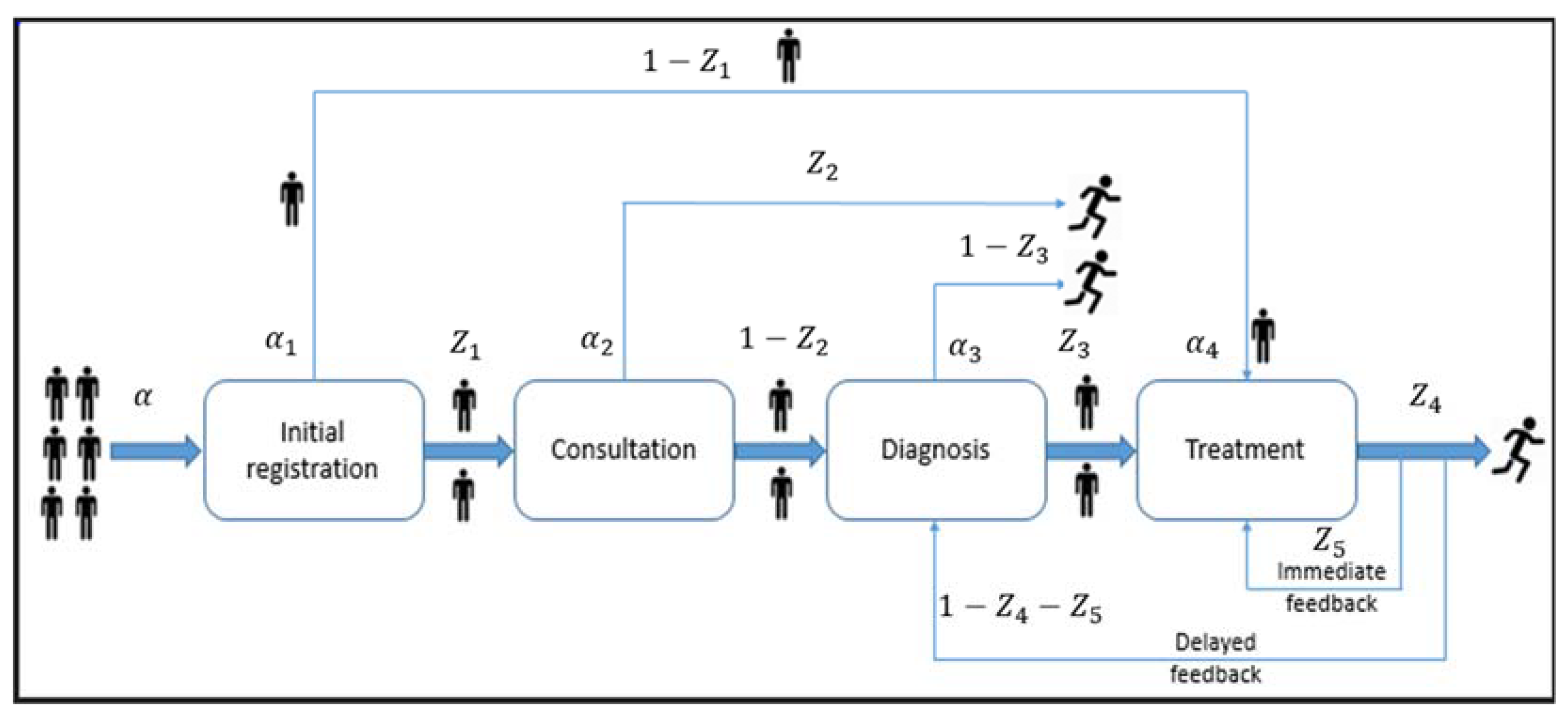
2. Models and Methods

This model proposes a store-and-forward telemedicine framework using an open queueing network consisting of four interconnected nodes. At node 1 (initial registration), patients arrive following a Poisson process with rate $\alpha$. Initial data registration is performed. If the case is urgent, the patient moves directly to node 4 (treatment) with probability $1-z_1$. If the case is non-urgent, the patient proceeds to node 2 (consultation) with probability $z_1$. Patients may leave the system after a basic consultation with probability $1-z_2$. If the patient requires additional diagnosis, they move forward to node 3 (Diagnosis) with probability $z_2$. After diagnosis, patients either proceed to node 4 (treatment) with probability $z_3$ or leave the system with probability $1-z_3$. This network structure includes the possibility that there is delayed feedback, where patients return to this node after treatment or consultation for further diagnosis. At node 4, patients receive treatment if necessary. After treatment, if the patient needs an additional consultation, they may go to immediate feedback with probability $z_5$. Both types of feedback are assumed to be independent of the state of the system.

It is assumed that both kinds of feedback are unaffected by the system’s current state. The four-state Markov process {$X_1\left(t\right),X_2\left(t\right),X_3\left(t{),X}_4\left(t\right) t\ge 0\right\}$ can be used to represent the system’s state, where $X_i\left(t\right)$ is the number of patients present at node ‘i’ at time ‘t’ (i = 1, 2, 3, 4). We aim to find the steady-state solution with $X_1$ patients at node 1, $X_2$ patients at node 2, $X_3$ patients at node 3, and $X_{4 }$ patients at node 4, represented by Q ($x_1,x_2,x_3,x_4)$. The average total arrival rate at each node is defined as rate ${\alpha }_i(i=1,2,3,4)$ using the local balance approach. Under steady-state conditions, the queueing network manages patient flow between nodes according to the specified probabilities. Every node operates as an M/M/1 queue, and performance parameters like average waiting times, average visits, and average patient counts are recorded at each node (Figure 1).

Assumptions:

To enable mathematical tractability and analytical clarity, the following assumptions are made in the proposed queueing network model of store-and-forward telemedicine.

• Single server at each node.
• Poisson Arrival process, exponential service time, open queueing network, fixed routing probabilities, feedback mechanisms, and symmetry in system behavior.

2.1. Notations

Table 1. Notations

Symbol	Description
$\alpha$	External Arrival rate to the system (Poisson arrival rate)
α1, α2, α3, α4	Arrival Rate at node 1, node 2, node 3, node 4.
β1, β2, β3, β4	Service Rate at node 1, node 2, node 3, node 4.
γ1, γ2, γ3, γ4	Traffic intensity (utilization factor) at nodes 1, 2, 3, 4.
$z_1,z_2,z_3,z_4,z_5$	Routing probabilities and immediate feedback
$x_1,x_2,x_3,x_4$	Number of patients at nodes 1, 2, 3, 4.
$R_1,R_2,R_{3,}{R}_4$	Average visit counts at nodes 1, 2, 3, 4.
$X_1,X_2,X_3,X_4$	Average number of patients at nodes 1, 2, 3, 4.
$S_1,S_2,S_3,S_4$	Average waiting time of customers at nodes 1, 2, 3, 4.
$Z\left(x_1,x_2,x_3,x_4\right)$	Joint probability of having patients x1, x2, x3, x4 at nodes 1, 2, 3, 4, respectively.
X	Total average number of customers in the system calculated as X = X1 + X2 + X3 + X4.
$S$	Total average waiting time for patients in the system S = S1 + S2 + S3 + S4.

shows some notations will be used in the following sections.

2.2. Balance Equation

For routing probabilities with feedback, the queueing network is represented here using four Markovian queueing models with Bernoulli schedules. We apply the conventional method of constructing the differential-difference equation from the system’s transient probabilities and inferring the balancing equation to obtain the steady-state solution of a model.

For each node, we define ${\alpha }_i(i=1,2,3,4)$ as the average total arrival rate using the basic balance approach.

The flow of patients through these nodes is governed by the following balance equations, where:

• ${\alpha }_i$ = total arrival rate at node i;
• $z_i$ = routing probabilities at specific transitions between nodes.

Node 1:

$${\alpha }_1=\alpha$$

(1)

Node 2:

$${\alpha }_2={\alpha }_1{z}_1$$

(2)

Node 3:

$${\alpha }_3={\alpha }_2\left(1-z_2\right)+{\alpha }_4\left(1-z_4-z_5\right)$$

(3)

Node 4:

$${\alpha }_4={\alpha }_1\left(1-z_1\right)+{\alpha }_3{z}_3+{\alpha }_4{z}_5.$$

(4)

Here $\alpha$, represents the external arrival rate of patients into the system (e.g., patients coming into the telemedicine network from outside).

${\alpha }_1$ is simply equal to $\alpha$ because node 1 is the entry point of the system, and all patients first go through initial registration.

After registration, patients move to consultation (node 2) with probability $z_1$. Thus, the arrival rate at node 2, ${\alpha }_2$ is the product of the arrival rate at node 1 and the transition probability $z_1.$ Patients come to diagnosis (node 3) from two sources: from consultation (node 2), if, after consultation, they do not immediately exit (probability $\left(1-z_2\right)$), or from treatment (node 4), if they require further diagnosis after initial treatment (probability ($\left(1-z_4-z_5\right)$. Therefore, patients include those moving from node 2 to node 3, those looping back from node 4 to node 3, and those directly transferring from initial registration (node 1), if their case is urgent and they do not go to consultation (probability (1 − z₁)). Patients then transfer from diagnosis (node 3), if treatment is needed after diagnosis (probability z₃). Feedback from treatment may lead to some patients not leaving immediately as they might require re-treatment or further processing (probability z₅).

Solving the above system of equations, we obtain the values of ${\alpha }_1,{\alpha }_2,{\alpha }_3,{\alpha }_4$:

$${\alpha }_1=\alpha$$

(5)

$${\alpha }_2=\alpha z_1$$

(6)

$${\alpha }_3={\displaystyle \frac{\alpha \left(1-z_1\right)\left(1-z_5\right)+\alpha \left(1-z_1\right)\left(1-z_4-z_5\right)}{\left(1-z_5\right)-z_3\left(1-z_4-z_5\right)}}$$

(7)

$${\alpha }_4={\displaystyle \frac{\alpha \left(1-z_1\right)+\frac{\alpha \left(1-z_1\right)\left(1-z_5\right)+\alpha \left(1-z_1\right)\left(1-z_4-z_5\right)}{\left(1-z_5\right)-z_3\left(1-z_4-z_5\right)}}{\left(1-z_5\right)}}$$

(8)

The Jackson network’s product-form solution provides a powerful method for analyzing the steady-state behavior of queueing networks. In an open queueing network under steady-state conditions and assuming Poisson arrivals and exponential service times, the joint probability distribution of the number of patients at each node can be factored into the product of the individual probabilities at each node. The Jackson network’s product form solution serves as the basis for the derivation of the joint probability for the number of patients in each node. It is possible to express the joint probability distribution as

$$Z\left(x_1,x_2,x_3,x_4\right)=Z\left(x_1\right)·Z\left(x_2\right)·Z\left(x_3\right)·Z\left(x_4\right)$$

(9)

Each $Z\left(x_i\right)$ is,

$$Z\left(x_i\right)=\left(1-{\gamma }_i\right){\gamma }_i^{x_i}, x_i\ge 0$$

(10)

where ${\gamma }_i={\displaystyle \frac{{\alpha }_i}{{\beta }_i}}$ is the utilization factor, ${\alpha }_i$ is the arrival rate at node $i$, and ${\beta }_i$ is the service rate at node $i$.

Thus, for a queueing network model with four nodes and two feedbacks, the steady state solution is as follows:

$$Z\left(x_1,x_2,x_3,x_4\right)=Z\left(x_1\right)·Z\left(x_2\right)·Z\left(x_3\right)·Z\left(x_4\right)$$

$$=(1-{\displaystyle \frac{{\alpha }_1}{{\beta }_1}})({{\displaystyle \frac{{\alpha }_1}{{\beta }_1}})}^{x_1}. (1-{\displaystyle \frac{{\alpha }_2}{{\beta }_2}})({{\displaystyle \frac{{\alpha }_2}{{\beta }_2}})}^{x_2}.(1-{\displaystyle \frac{{\alpha }_3}{{\beta }_3}}\left)\right({{\displaystyle \frac{{\alpha }_3}{{\beta }_3}})}^{x_3}.(1-{\displaystyle \frac{{\alpha }_4}{{\beta }_4}})({{\displaystyle \frac{{\alpha }_4}{{\beta }_4}})}^{x_4}$$

$$=(1-{\displaystyle \frac{\alpha }{{\beta }_1}})({{\displaystyle \frac{\alpha }{{\beta }_1}})}^{x_1}.(1-{\displaystyle \frac{\alpha z_1}{{\beta }_2}})({{\displaystyle \frac{\alpha z_1}{{\beta }_2}})}^{x_2}. \left(1-{\displaystyle \frac{\frac{\alpha \left(1-z_1\right)\left(1-z_5\right)+\alpha \left(1-z_1\right)\left(1-z_4-z_5\right)}{\left(1-z_5\right)-z_3\left(1-z_4-z_5\right)}}{{\beta }_3}}\right)$$

(11)

$$\times ({{\displaystyle \frac{\frac{\alpha \left(1-z_1\right)\left(1-z_5\right)+\alpha \left(1-z_1\right)\left(1-z_4-z_5\right)}{\left(1-z_5\right)-z_3\left(1-z_4-z_5\right)}}{{\beta }_3}})}^{x_3}.$$

$$\times (1-{\displaystyle \frac{\frac{\alpha \left(1-z_1\right)+\frac{\alpha \left(1-z_1\right)\left(1-z_5\right)+\alpha \left(1-z_1\right)\left(1-z_4-z_5\right)}{\left(1-z_5\right)-z_3\left(1-z_4-z_5\right)}}{\left(1-z_5\right)}}{{\beta }_4}})({{\displaystyle \frac{\frac{\alpha \left(1-z_1\right)+\frac{\alpha \left(1-z_1\right)\left(1-z_5\right)+\alpha \left(1-z_1\right)\left(1-z_4-z_5\right)}{\left(1-z_5\right)-z_3\left(1-z_4-z_5\right)}}{\left(1-z_5\right)}}{{\beta }_4}})}^{x_4}$$

2.3. Measuring Network Performance

Using these flows and state distributions, the network performance metrics that follow are calculated. Throughput is defined as the average arrival rate of an external Poisson process entering the network to the ith queue $Q_i$, where i = 1, 2, 3, 4. Thus, overall throughput is equal to the total external arrival rate or $\alpha$.

2.3.1. Average Visit Count to Nodes

Let $R_i$ be the visit count to node $i\left(i=1, 2, 3, 4\right)$. Then:

$$R_1={\displaystyle \frac{{\alpha }_1}{total throughput}}={\displaystyle \frac{\alpha }{\alpha }}=1;$$

(12)

$$R_2={\displaystyle \frac{{\alpha }_2}{total throughput}}={\displaystyle \frac{\mathit{\alpha }{\mathit{z}}_1}{\alpha }}=z_1;$$

(13)

$$R_3={\displaystyle \frac{{\alpha }_3}{total throughput}}={\displaystyle \frac{{\alpha }_3}{\alpha }}={\displaystyle \frac{\frac{\mathit{\alpha }\left(1-{\mathit{z}}_1\right)\left(1-{\mathit{z}}_5\right)+\mathit{\alpha }\left(1-{\mathit{z}}_1\right)\left(1-{\mathit{z}}_4-{\mathit{z}}_5\right)}{\left(1-{\mathit{z}}_5\right)-{\mathit{z}}_3\left(1-{\mathit{z}}_4-{\mathit{z}}_5\right)}}{\alpha }}$$

$$={\displaystyle \frac{\left(1-z_1\right)\left(1-z_5\right)+\left(1-z_1\right)\left(1-z_4-z_5\right)}{\left(1-z_5\right)-z_3\left(1-z_4-z_5\right)}} ;$$

(14)

$$R_4={\displaystyle \frac{{\alpha }_4}{total throughput}}={\displaystyle \frac{\mathit{\alpha }\left(\mathbf{1}-{\mathit{z}}_{\mathbf{1}}\right)+\frac{\mathit{\alpha }\left(\mathbf{1}-{\mathit{z}}_{\mathbf{1}}\right)\left(\mathbf{1}-{\mathit{z}}_{\mathbf{5}}\right)+\mathit{\alpha }\left(\mathbf{1}-{\mathit{z}}_{\mathbf{1}}\right)\left(\mathbf{1}-{\mathit{z}}_{\mathbf{4}}-{\mathit{z}}_{\mathbf{5}}\right)}{\left(\mathbf{1}-{\mathit{z}}_{\mathbf{5}}\right)-{\mathit{z}}_{\mathbf{3}}\left(\mathbf{1}-{\mathit{z}}_{\mathbf{4}}-{\mathit{z}}_{\mathbf{5}}\right)}}{\mathit{\alpha }\left(\mathbf{1}-{\mathit{z}}_{\mathbf{5}}\right)}}.$$

(15)

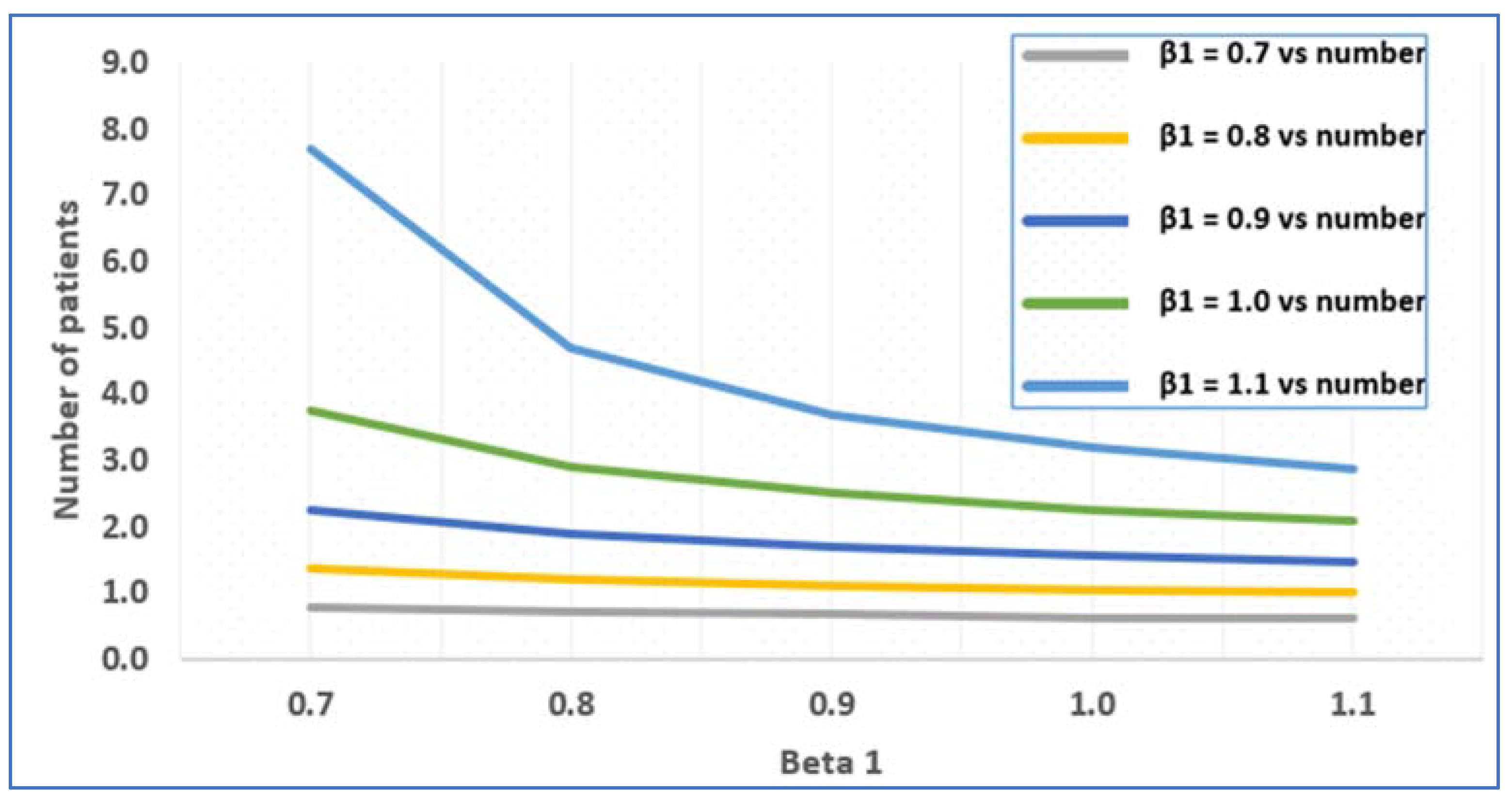
2.3.2. Average Number of Patients in the System

The average numbers of patients in the four nodes are calculated below. Let $X_i\left(i=1, 2, 3, 4\right)$ be the average number of patients in queue $Q_i\left(i=1, 2, 3, 4\right)$

$$X_1={\displaystyle \frac{{\gamma }_1}{1-{\gamma }_1}}={\displaystyle \frac{\frac{{\mathit{\alpha }}_{\mathbf{1}}}{{\mathit{\beta }}_{\mathbf{1}}}}{\left(\mathbf{1}-\frac{{\mathit{\alpha }}_{\mathbf{1}}}{{\mathit{\beta }}_{\mathbf{1}}}\right)}} ={\displaystyle \frac{\alpha }{{\beta }_1-\alpha }};$$

(16)

$$X_2={\displaystyle \frac{{\gamma }_2}{1-{\gamma }_2}}={\displaystyle \frac{\frac{{\mathit{\alpha }}_{\mathbf{2}}}{{\mathit{\beta }}_{\mathbf{2}}}}{\left(\mathbf{1}-\frac{{\mathit{\alpha }}_{\mathbf{2}}}{{\mathit{\beta }}_{\mathbf{2}}}\right)}} ={\displaystyle \frac{\mathit{\alpha }{\mathit{z}}_{\mathbf{1}}}{{\mathit{\beta }}_{\mathbf{2}}-\mathit{\alpha }{\mathit{z}}_{\mathbf{1}}}};$$

(17)

$$X_3={\displaystyle \frac{{\gamma }_3}{1-{\gamma }_3}}={\displaystyle \frac{\frac{{\mathit{\alpha }}_{\mathbf{3}}}{{\mathit{\beta }}_{\mathbf{3}}}}{\left(\mathbf{1}-\frac{{\mathit{\alpha }}_{\mathbf{3}}}{{\mathit{\beta }}_{\mathbf{3}}}\right)}}={\displaystyle \frac{{\alpha }_3}{{\beta }_3-{\alpha }_3}}={\displaystyle \frac{\frac{\mathit{\alpha }\left(\mathbf{1}-{\mathit{z}}_{\mathbf{1}}\right)\left(\mathbf{1}-{\mathit{z}}_{\mathbf{5}}\right)+\mathit{\alpha }\left(\mathbf{1}-{\mathit{z}}_{\mathbf{1}}\right)\left(\mathbf{1}-{\mathit{z}}_{\mathbf{4}}-{\mathit{z}}_{\mathbf{5}}\right)}{\left(\mathbf{1}-{\mathit{z}}_{\mathbf{5}}\right)-{\mathit{z}}_{\mathbf{3}}\left(\mathbf{1}-{\mathit{z}}_{\mathbf{4}}-{\mathit{z}}_{\mathbf{5}}\right)}}{{\beta }_{\mathbf{3}}-\frac{\mathit{\alpha }\left(\mathbf{1}-{\mathit{z}}_{\mathbf{1}}\right)\left(\mathbf{1}-{\mathit{z}}_{\mathbf{5}}\right)+\mathit{\alpha }\left(\mathbf{1}-{\mathit{z}}_{\mathbf{1}}\right)\left(\mathbf{1}-{\mathit{z}}_{\mathbf{4}}-{\mathit{z}}_{\mathbf{5}}\right)}{\left(\mathbf{1}-{\mathit{z}}_{\mathbf{5}}\right)-{\mathit{z}}_{\mathbf{3}}\left(\mathbf{1}-{\mathit{z}}_{\mathbf{4}}-{\mathit{z}}_{\mathbf{5}}\right)}}}$$

(18)

$$X_4={\displaystyle \frac{{\gamma }_4}{1-{\gamma }_4}}={\displaystyle \frac{\frac{{\mathit{\alpha }}_{\mathbf{4}}}{{\mathit{\beta }}_{\mathbf{4}}}}{\left(\mathbf{1}-\frac{{\mathit{\alpha }}_{\mathbf{4}}}{{\mathit{\beta }}_{\mathbf{4}}}\right)}}={\displaystyle \frac{\frac{\mathit{\alpha }\left(\mathbf{1}-{\mathit{z}}_{\mathbf{1}}\right)+\frac{\mathit{\alpha }\left(\mathbf{1}-{\mathit{z}}_{\mathbf{1}}\right)\left(\mathbf{1}-{\mathit{z}}_{\mathbf{5}}\right)+\mathit{\alpha }\left(\mathbf{1}-{\mathit{z}}_{\mathbf{1}}\right)\left(\mathbf{1}-{\mathit{z}}_{\mathbf{4}}-{\mathit{z}}_{\mathbf{5}}\right)}{\left(\mathbf{1}-{\mathit{z}}_{\mathbf{5}}\right)-{\mathit{z}}_{\mathbf{3}}\left(\mathbf{1}-{\mathit{z}}_{\mathbf{4}}-{\mathit{z}}_{\mathbf{5}}\right)}}{\left(\mathbf{1}-{\mathit{z}}_{\mathbf{5}}\right)}}{{\beta }_{\mathbf{4}}-\frac{\mathit{\alpha }\left(\mathbf{1}-{\mathit{z}}_{\mathbf{1}}\right)+\frac{\mathit{\alpha }\left(\mathbf{1}-{\mathit{z}}_{\mathbf{1}}\right)\left(\mathbf{1}-{\mathit{z}}_{\mathbf{5}}\right)+\mathit{\alpha }\left(\mathbf{1}-{\mathit{z}}_{\mathbf{1}}\right)\left(\mathbf{1}-{\mathit{z}}_{\mathbf{4}}-{\mathit{z}}_{\mathbf{5}}\right)}{\left(\mathbf{1}-{\mathit{z}}_{\mathbf{5}}\right)-{\mathit{z}}_{\mathbf{3}}\left(\mathbf{1}-{\mathit{z}}_{\mathbf{4}}-{\mathit{z}}_{\mathbf{5}}\right)}}{\left(\mathbf{1}-{\mathit{z}}_{\mathbf{5}}\right)}}}$$

(19)

The average number of patients in the overall system, $X$, is calculated by:

$$X=X_1+X_2+X_3+X_4.$$

(20)

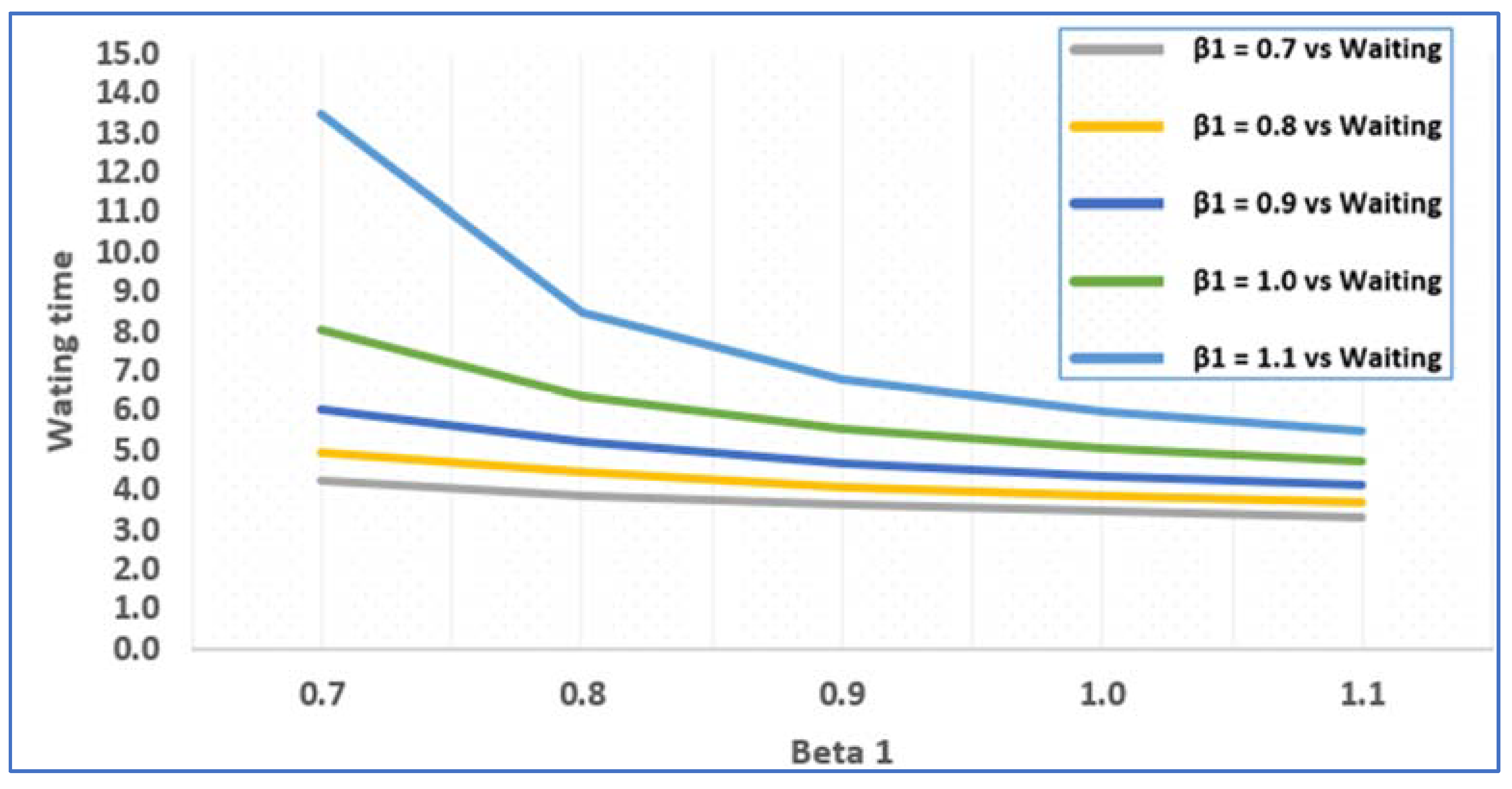
2.3.3. Average Waiting Time of a Patient at Each Node

A patient’s average waiting time is the amount of time they spend in the system overall before leaving the queueing network. The total amount of time a patient spends in each of the network’s four nodes can be used to determine this in one of two ways. The direct use of Little’s formula is another method that can be used.

If $S_i$ is the average waiting time of a patient at node $i \left(i=1, 2, 3, 4\right),$ then:

$$S_1={\displaystyle \frac{R_1{X}_1}{{\alpha }_1}};$$

(21)

$$S_2={\displaystyle \frac{R_2{X}_2}{{\alpha }_2}};$$

(22)

$$S_3={\displaystyle \frac{R_3{X}_3}{{\alpha }_3}};$$

(23)

$$S_4={\displaystyle \frac{R_4{X}_4}{{\alpha }_4}},$$

(24)

where:

$${\alpha }_1=\alpha ;$$

(25)

$${\alpha }_2=\alpha z_1;$$

(26)

$${\alpha }_3={\displaystyle \frac{\mathsf{\alpha }\left(1-{\mathrm{z}}_1\right)\left(1-{\mathrm{z}}_5\right)+\mathsf{\alpha }\left(1-{\mathrm{z}}_1\right)\left(1-{\mathrm{z}}_4-{\mathrm{z}}_5\right)}{\left(1-{\mathrm{z}}_5\right)-{\mathrm{z}}_3\left(1-{\mathrm{z}}_4-{\mathrm{z}}_5\right)}};$$

(27)

$${\alpha }_4={\displaystyle \frac{\mathsf{\alpha }\left(1-{\mathrm{z}}_1\right)+\frac{\mathsf{\alpha }\left(1-{\mathrm{z}}_1\right)\left(1-{\mathrm{z}}_5\right)+\mathsf{\alpha }\left(1-{\mathrm{z}}_1\right)\left(1-{\mathrm{z}}_4-{\mathrm{z}}_5\right)}{\left(1-{\mathrm{z}}_5\right)-{\mathrm{z}}_3\left(1-{\mathrm{z}}_4-{\mathrm{z}}_5\right)}}{\left(1-{\mathrm{z}}_5\right)}} .$$

(28)

In the overall system, the average waiting time of a patient is calculated by

$$\mathit{S}={\mathit{S}}_{\mathbf{1}}+{\mathit{S}}_{\mathbf{2}}+{\mathit{S}}_{\mathbf{3}}+{\mathit{S}}_{\mathbf{4}}.$$

(29)

3. Results

3.1. Numerical Illustration

The arrival rate and service rate have exponential distributions with $\alpha$ and $\beta$, respectively. We determined the steady-state solution and performance metrics values using MATLAB 2020. The following tables present the performance metrics and steady state probabilities calculated for parametric values (

Table 2. Average visit count to nodes.

${\mathit{R}}_1$	${\mathit{R}}_2$	${\mathit{R}}_3$	${\mathit{R}}_4$
1	0.3	1.82	1.97

,

Table 3. Average number of patients in the system.

${\mathit{X}}_1$	${\mathit{X}}_2$	${\mathit{X}}_3$	${\mathit{X}}_4$	$\mathit{X}$
0.667	0.0937	1.542	0.9559	3.2586

,

Table 4. Average waiting time of a patient at each node.

${\mathit{S}}_1$	${\mathit{S}}_2$	${\mathit{S}}_3$	${\mathit{S}}_4$	$\mathit{S}$
3.335	0.4685	7.71	4.816	16.3295

and

Table 5. Steady-state distribution.

$\left({\mathit{x}}_1,{\mathit{x}}_2,{\mathit{x}}_3,{\mathit{x}}_4\right)$	$\mathit{Z}\left({\mathit{x}}_1,{\mathit{x}}_2,{\mathit{x}}_3,{\mathit{x}}_4\right)$	$\left({\mathit{x}}_1,{\mathit{x}}_2,{\mathit{x}}_3,{\mathit{x}}_4\right)$	$\mathit{Z}\left({\mathit{x}}_1,{\mathit{x}}_2,{\mathit{x}}_3,{\mathit{x}}_4\right)$
(0 0 0 0)	0.36206	$\left(4 3 1 0\right)$	0.0000003
$\left(1 0 0 0\right)$	0.01448	$\left(0 4 1 0\right)$	0.000001
$\left(2 0 0 0\right)$	0.00579	$\left(1 4 1 0\right)$	0.0000004
$\left(3 0 0 0\right)$	0.00232	$\left(2 4 1 0\right)$	0.0000002
$\left(4 0 0 0\right)$	0.00093	$\left(3 4 1 0\right)$	0.00000007
$\left(0 1 0 0\right)$	0.00310	$\left(4 4 1 0\right)$	0.00000002
$\left(1 1 0 0\right)$	0.00124	$\left(0 0 2 0\right)$	0.011354
$\left(2 1 0 0\right)$	0.00050	$\left(1 0 2 0\right)$	0.004542
$\left(3 1 0 0\right)$	0.00019	$\left(2 0 2 0\right)$	0.001816
$\left(4 1 0 0\right)$	0.000079	$\left(3 0 2 0\right)$	0.00073
$\left(0 2 0 0\right)$	0.00027	$\left(4 0 2 0\right)$	0.00029
$\left(1 2 0 0\right)$	0.00014	$\left(0 1 2 0\right)$	0.000973
$\left(2 2 0 0\right)$	0.000042	$\left(1 1 2 0\right)$	0.00038
$\left(3 2 0 0\right)$	0.000017	$\left(2 1 2 0\right)$	0.00015
$\left(4 2 0 0\right)$	0.0000068	$\left(3 1 2 0\right)$	0.000062
$\left(0 3 0 0\right)$	0.0000228	$\left(4 1 2 0\right)$	0.000025
$\left(1 3 0 0\right)$	0.0000091	$\left(0 2 2 0\right)$	0.000083
$\left(2 3 0 0\right)$	0.0000036	$\left(1 2 2 0\right)$	0.000033
$\left(3 3 0 0\right)$	1.4592 × 10−6	$\left(2 2 2 0\right)$	0.000013
$\left(4 3 0 0\right)$	5.8368 × 10−7	$\left(3 2 2 0\right)$	0.000005
$\left(0 4 0 0\right)$	1.954 × 10−6	$\left(4 2 2 0\right)$	2.13555 × 10−6
$\left(1 4 0 0\right)$	7.817 × 10−7	$\left(0 3 2 0\right)$	7.15015 × 10−6
$\left(2 4 0 0\right)$	3.1269 × 10−7	$\left(1 3 2 0\right)$	0.000973
$\left(3 4 0 0\right)$	1.2505 × 10−7	$\left(2 3 2 0\right)$	1.1445 × 10−6
$\left(4 4 0 0\right)$	5.003 × 10−8	$\left(3 3 2 0\right)$	4.57615 × 10−7
$\left(0 0 1 0\right)$	0.02027	$\left(4 3 2 0\right)$	1.83045 × 10−7
$\left(1 0 1 0\right)$	0.00811	$\left(2 4 4 1\right)$	2.61395 × 10−8
$\left(2 0 1 0\right)$	0.00324	$\left(3 4 4 1\right)$	1.04555 × 10−8
$\left(3 0 1 0\right)$	0.00129	$\left(4 4 4 1\right)$	4.18225 × 10−9
$\left(4 0 1 0\right)$	0.000520	$\left(0 4 4 2\right)$	1.38865 × 10−7
$\left(0 1 10\right)$	0.000175	$\left(1 4 4 2\right)$	5.55445 × 10−8
$\left(1 1 1 0\right)$	0.00070	$\left(2 4 4 2\right)$	2.22185 × 10−8
$\left(2 1 1 0\right)$	0.00028	$\left(3 4 4 2\right)$	8.88715 × 10−9
$\left(3 1 1 0\right)$	0.00011	$\left(4 4 4 2\right)$	3.55485 × 10−9
$\left(4 1 1 0\right)$	4.4495 × 10−5	$\left(0 4 4 3\right)$	1.18035 × 10−7
$\left(0 2 1 0\right)$	0.000148	$\left(1 4 4 3\right)$	4.72135 × 10−8
$\left(1 2 1 0\right)$	5.95845 × 10−5	$\left(2 4 4 3\right)$	1.88855 × 10−8
$\left(2 2 1 0\right)$	2.38345 × 10−5	$\left(3 4 4 3\right)$	7.5545 × 10−9
$\left(3 2 1 0\right)$	9.53355 × 10−6	$\left(4 4 4 3\right)$	3.02165 × 10−9
$\left(4 2 1 0\right)$	3.81345 × 10−6	$\left(0 4 4 4\right)$	1.00335 × 10−7
$\left(0 3 1 0\right)$	1.27685 × 10−5	$\left(1 4 4 4\right)$	4.01315 × 10−8
$\left(1 3 1 0\right)$	5.1075 × 10−6	$\left(2 4 4 4\right)$	1.60525 × 10−8
$\left(2 3 1 0\right)$	2.04295 × 10−6	$\left(3 4 4 4\right)$	6.42095 × 10−9
$\left(3 3 1 0\right)$	8.17165 × 10−7	$\left(4 4 4 4\right)$	2.56845 × 10−9

).

$$\begin{gathered} \alpha =0.2, z_1=0.3, z_2=0.2, z_3=0.4, z_4=0.2, z_5=0.3, {\beta }_1=0.5, {\beta }_2=0.7, \\ {\beta }_3=0.6, {\beta }_4=0.8. \end{gathered}$$

In order to determine the system’s behaviour by fixing the probability and service rate ${\beta }_1, {\beta }_2{, \beta }_3, {\beta }_4,$ the following cases are examined in relation to the parameters defined below.

• Case 1:

$$\alpha =0.2, z_1=0.3, z_2=0.2, z_3=0.4, z_4=0.2, z_5=0.3, {\beta }_1=0.7, {\beta }_2=1.2, {\beta }_3=2.2, {\beta }_4=3.2.$$

For the case where the input rate $\alpha$ increases from 0.2 to 0.6, and the service rate of the first queue ${\beta }_1$ increases from 0.7 to 1.1, the average number of patients at each node and the average waiting time of patients in the system are calculated using MATLAB. It is clear from the above graph that when the service rate increases, the average number of patients in the system and the average waiting time of a patient at each node increase. This shows how the average number of patients in the system and the input arrival rate are related. The matching values are shown in the following figures (Figure 2 and Figure 3).

• Case 2:

$$\alpha =0.2, z_1=0.3, z_2=0.2, z_3=0.4, z_4=0.2, z_5=0.3, {\beta }_1=0.7, {\beta }_2=1.2, {\beta }_3=2.2, {\beta }_4=3.2.$$

For the case where the input rate $\alpha$ increases from 0.2 to 0.6, and the service rate of the first queue ${\beta }_1$ increases from 0.7 to 1, the average number of patients and the average waiting time are calculated using MATLAB. It is clear from the above graph that when the service rate increases, the average number of patients in the system and the average waiting time of a patient at each node decrease. This shows the correlation between the average number of patients in the system and the input arrival rate. The appropriate values are shown in the following figures (Figure 4 and Figure 5).

3.2. Graph-Theoretic Approach of Queueing Network

3.2.1. Description of the Model

The definition of a graph G, given an ordered pair G = (V,E), is as follows. As V = {$v_1,v_2,\dots v_n\}$, V is a collection of vertices, sometimes referred to as nodes, or points, known as edges, links, or arcs. E is a group of pairs of vertices represented as the relationship between u and v, e = {u,v}. An undirected graph is one in which there is no directionality among its edges {u,v} = {v,u}. A social network where friendships are reciprocal is one example. A directed graph is one in which each edge has a specific direction $\left\{u,v\right\} \ne \{v,u\}$. For instance, following on Twitter does not always entail reciprocity. A graph that has weight (values) attached to its edges—which frequently indicate costs, distances, or capacities—is said to be weighted. For instance, a road network with distances.

A subset of graph G that has all its vertices connected by the fewest number of edges is called a spanning tree. This makes use of the fewest edges required to maintain connectivity between all vertices. A graph with n vertices will have precisely (n − 1) edges in its spanning tree. There can be more than one legitimate spanning tree in a graph. The spanning tree needs to be acyclic and connected. The directed graphs represented in this model exhibit structural symmetry, which refers to the behaviour of the nodes.

Counting spanning trees is an important topic in enumerative combinatory. The typical approach employs determinants, and an explicit formula has been discovered for various families of directed and undirected graphs. We focused on the directed graph for this model. A directed graph is one in which edges have direction and represent relationships between nodes. We propose a new method for calculating the number of spanning trees at each given node, and we demonstrate how this produces steady-state queue length probability.

In this model, we have considered Figure 1 as a directed graph where nodes are considered as vertices and edges represent the transition probabilities between the nodes. An edge from node 1 (vertex 1) to node 2 (vertex 2) has weight $z_1=0.3$ and from node 2 to node 3 has weight $z_2=0.2,$ and similarly for other nodes (Figure 6).

Hence, using the theorem below, we will find the steady-state probability.

Theorem 1.

The steady state probabilities for any discrete time Markov Chain are related by a constant factor to the number of spanning trees rooted at the node of the associated graph [22].

Consider the transition matrix from Figure 1

$$\mathrm{Transition} \mathrm{matrix}=\left[\begin{array}{cc}\begin{array}{cc} 0& 1\\ 0& 0\end{array}& \begin{array}{cc}0 & \begin{array}{cc}0 & 0\end{array}\\ p_1 & \begin{array}{cc}0& 1-p_1\end{array}\end{array}\\ \begin{array}{cc}1-p_2& 0\\ \begin{array}{c}1-p_3\\ p_4\end{array}& \begin{array}{c}0\\ 0\end{array}\end{array}& \begin{array}{cc}0& \begin{array}{cc}{p}_2& 0 \end{array}\\ \begin{array}{c}0\\ 0\end{array}& \begin{array}{cc}\begin{array}{c}0 \\ 1-p_4-p_5\end{array}& \begin{array}{c}{p}_3\\ p_5\end{array}\end{array}\end{array}\end{array}\right].$$

The steady-state probabilities $\pi ={\pi }_1,{\pi }_2,\dots .,{\pi }_n$ should satisfy $\pi Z=\pi$ and ${\sum }_{i=1}^n{\pi }_i=1$.

Hence, by taking values $z_1=0.3, z_2=0.2, z_3=0.4, z_4=0.2, z_5=0.3,$ we obtain

$$\mathrm{Z}=\left[\begin{array}{cc}\begin{array}{cc} 0& 1\\ 0& 0\end{array}& \begin{array}{cc}0 & \begin{array}{cc}0 & 0 \end{array}\\ 0.3 & \begin{array}{cc}0 & 0.7\end{array}\end{array}\\ \begin{array}{cc}0.8& 0\\ \begin{array}{c}0.6\\ 0.2\end{array}& \begin{array}{c}0\\ 0\end{array}\end{array}& \begin{array}{cc} 0& \begin{array}{cc}0.2 & 0\end{array}\\ \begin{array}{c}0\\ 0\end{array}& \begin{array}{c} \begin{array}{cc}0& 0.4\end{array}\\ \begin{array}{cc}0.5 & 0.3\end{array}\end{array}\end{array}\end{array}\right]$$

$$\left[{\pi }_0,{\pi }_1,{\pi }_2,{\pi }_3,{\pi }_4\right]\left[\begin{array}{cc}\begin{array}{cc} 0& 1\\ 0& 0\end{array}& \begin{array}{cc}0 & \begin{array}{cc}0 & 0 \end{array}\\ 0.3 & \begin{array}{cc}0 & 0.7\end{array}\end{array}\\ \begin{array}{cc}0.8& 0\\ \begin{array}{c}0.6\\ 0.2\end{array}& \begin{array}{c}0\\ 0\end{array}\end{array}& \begin{array}{cc} 0& \begin{array}{cc}0.2 & 0\end{array}\\ \begin{array}{c}0\\ 0\end{array}& \begin{array}{c} \begin{array}{cc}0& 0.4\end{array}\\ \begin{array}{cc}0.5 & 0.3\end{array}\end{array}\end{array}\end{array}\right] = \left[{\pi }_0,{\pi }_1,{\pi }_2,{\pi }_3,{\pi }_4\right]$$

$$0.8{\pi }_2+0.6{\pi }_3+0.2{\pi }_4={\pi }_0$$

$${\pi }_0={\pi }_1$$

$$0.3{\pi }_1={\pi }_2$$

$$0.2{\pi }_2+0.5{\pi }_4={\pi }_3$$

$$0.7{\pi }_1+0.4{\pi }_3+0.3{\pi }_4={\pi }_4$$

Using MATLAB and solving the above equations, we obtain the steady-state probabilities

$${\pi }_0=0.2207, {\pi }_1=0.2207, {\pi }_2=0.0662, {\pi }_3=0.1730, {\pi }_4=0.3195.$$

3.2.2. Graph Representation

The Markov chain can be represented as a directed graph G, where nodes correspond to the states.

A directed edge from $i\mathrm{t}\mathrm{o} j$ exists if $p_{ij}>0$

$$\left[{\pi }_0 {\pi }_1 {\pi }_2 {\pi }_3{ \pi }_4 \right]$$

Now, using the above theorem, consider the transition probabilities:

$$Z=\left[\begin{array}{cc}\begin{array}{cc} 0& 1\\ 0& 0\end{array}& \begin{array}{cc}0 & \begin{array}{cc}0 & 0 \end{array}\\ 0.3 & \begin{array}{cc}0 & 0.7\end{array}\end{array}\\ \begin{array}{cc}0.8& 0\\ \begin{array}{c}0.6\\ 0.2\end{array}& \begin{array}{c}0\\ 0\end{array}\end{array}& \begin{array}{cc} 0& \begin{array}{cc}0.2 & 0\end{array}\\ \begin{array}{c}0\\ 0\end{array}& \begin{array}{c} \begin{array}{cc}0& 0.4\end{array}\\ \begin{array}{cc}0.5 & 0.3\end{array}\end{array}\end{array}\end{array}\right]$$

The Laplacian matrix L is defined by the relation L $=D-Z$ $\mathrm{w}\mathrm{h}\mathrm{e}\mathrm{r}\mathrm{e} D$ is the unit 5 × 5 matrix:

$$L= \left[\begin{array}{ccccc}1& 0& 0& 0& 0\\ 0& 1& 0& 0& 0\\ 0& 0& 1& 0& 0\\ 0& 0& 0& 1& 0\\ 0& 0& 0& 0& 1\end{array}\right]-\left[\begin{array}{cc}\begin{array}{cc} 0& 1\\ 0& 0\end{array}& \begin{array}{cc}0 & \begin{array}{cc}0 & 0 \end{array}\\ 0.3 & \begin{array}{cc}0 & 0.7\end{array}\end{array}\\ \begin{array}{cc}0.8& 0\\ \begin{array}{c}0.6\\ 0.2\end{array}& \begin{array}{c}0\\ 0\end{array}\end{array}& \begin{array}{cc} 0& \begin{array}{cc}0.2 & 0\end{array}\\ \begin{array}{c}0\\ 0\end{array}& \begin{array}{c} \begin{array}{cc}0& 0.4\end{array}\\ \begin{array}{cc}0.5 & 0.3\end{array}\end{array}\end{array}\end{array}\right]$$

Kirchhoff’s theorem, also known as the matrix-tree theorem, is a fundamental result in graph theory. It is a method to calculate the number of spanning trees in a connected graph using its Laplacian matrix.

Let G be a graph with n vertices that is linked and undirected. Any cofactor of the Laplacian matrix L of G has a determinant that indicates how many spanning trees there are in G. To apply Kirchhoff’s theorem, we remove one row and one column from L to obtain the matrix of minors $L_{minor}=0.5$. This is the determinant of the matrix (or the number of spanning trees rooted at node $\left(s_1\right).$ Similarly for $s_2,s_3,s_4,s_5)$, we remove the second row and column:

$$L_{minor}=0.5; 0.15; 0.39; 0.72$$

Therefore, the number of spanning trees rooted at $s_1$ and $s_2,s_3,s_4,s_5$ are proportional to the transition probabilities. The steady-state probabilities are proportional to the spanning tree, so,

$${\pi }_0~ 0.5 ; {\pi }_1~ 0.5 ; {\pi }_2~0.15 ; {\pi }_3~0.39 ; {\pi }_4~ 0.72 .$$

After some calculus, the total weight is: ${\pi }_0=0.2207;{\pi }_1=0.2207;{\pi }_2=0.0662;{\pi }_3=0.1730;{\pi }_4=0.3195$.

Hence, the steady-state probabilities are found same using a graph-theoretic approach.

4. Conclusions

Using store-and-forward telemedicine as an open queueing network with four nodes and two types of feedback, we investigated the healthcare system in emergency situations in rural areas. The system’s steady-state behaviour and performance parameters, including average visit count, average patient waiting time, and average patient number, are expressed directly. The numerical values are calculated using MATLAB. A numerical example is presented for illustration. The analysis demonstrated how changes in key parameters such as arrival rates, service rates, and routing probabilities influence overall system performance. Symmetry is important for patient flow and system stability in our store-and-forward telemedicine network. In this network, the service times of all nodes are identical. The probability of moving from one node to another node is also the same. The future work is to generalize the model to include multiple servers at each node and patients of different cases with varying service requirements. This model highlights the utility of queueing network theory combined with graph-theoretic methods.

References

1. Sreekala, M.S. Study on Queueing Networks and Their Applications; Department of Statistics, University of Calicut: Malappuram, India, 2016. [Google Scholar]
2. Pandian, P.S.; Safeer, K.P.; Shakunthala, D.T.I.; Gopal, P.; Padaki, V.C. Store and Forward Applications in Telemedicine for Wireless IP Based Networks. J. Netw. 2007, 2, 58–65. [Google Scholar] [CrossRef]
3. Alenany, E.; Adel El-Baz, M. Modelling a hospital as a queueing network: Analysis for improving performance. Int. J. Ind. Manuf. Eng. 2017, 11, 1181–1187. [Google Scholar]
4. Smith, J.M. Introduction to Queueing Networks: Theory Practice; Springer: Berlin/Heidelberg, Germany, 2018. [Google Scholar]
5. Gupta, R.; Gamad, R.S.; Bansod, P. Telemedicine: A brief analysis. Cogent Eng. 2014, 1, 966459. [Google Scholar] [CrossRef]
6. Gross, D.; Shortie, J.F.; Thompson, J.M.; Harris, C.M. Fundamentals of Queueing Theory, 4th ed.; John Wiley & Sons, Inc.: Hoboken, NJ, USA, 2008. [Google Scholar]
7. Thangaraj, V.; Vanitha, S. On the analysis of M/M/1 feedback queue with Catastrophes using continued fractions. Int. J. Pure Appl. Math. 2009, 53, 133–151. [Google Scholar]
8. Gaston, E.A. Telemedicne—Is Ben Boon. JAMA—J. Am. Med. Assoc. 1964, 188, 329. [Google Scholar] [CrossRef]
9. Bird, K.T.; Murphy, R.L.H.; Cohen, G.L. Telemedicine and Future of Pulmonary Disease. Dis. Chest 1969, 56, 242. [Google Scholar]
10. Dean, N.; Kelmans, A.K.; Lih, K.; Massey, W.A. The Spanning Tree Enumeration Problem for Digraphs; Princeton University: Princeton, NJ, USA, 1999. [Google Scholar]
11. Brown, F.W. Rural telepsychiatry. Psychiatr. Serv. 1998, 49, 963–964. [Google Scholar] [CrossRef]
12. Holzer, W.H. Telemedicine—New Application of Communications Technology. IEEE Transac. Commun. 1974, 22, 685–688. [Google Scholar] [CrossRef]
13. Clifford, M.H. One-UPMANSHIP in Telemedicine. IEEE Trans. Aerosp. Electron. Syst. 1973, AES9(5), 805–806. [Google Scholar]
14. Park, B.; Bashshur, R. Some Implication of Telemedicine. J. Commun. 1975, 25, 161–166. [Google Scholar] [CrossRef]
15. Grundly, B.L. Telemedicine in Critical Care—Preliminary Report. Crit. Care Med. 1976, 4, 104–105. [Google Scholar] [CrossRef]
16. Allan, R. Medical Electronics Coming—Era of Telemedicine. IEEE Spectr. 1976, 13, 30–35. [Google Scholar]
17. Scholl, J.; Lambrinos, L.; Lindgren, A. Rural telemedicine networks using store-and-forward Voice-over-IP. Stud. Health Technol. Inform. 2009, 150, 448–452. [Google Scholar]
18. Berge, C. Graphs and Hypergraph, 2nd ed.; North-Holland: Amsterdam, The Netherlands, 1989. [Google Scholar]
19. Gabow, H.N.; Myers, W.W. Finding all spanning trees of directed and undirected graphs. SIAM J. Comput. 1978, 7, 280–287. [Google Scholar] [CrossRef]
20. Pandian, P.S. An Overview of Telemedicine Technologies for Healthcare Applications. Int. J. Biomed. Clin. Eng. 2016, 5, 29–52. [Google Scholar] [CrossRef]
21. Chen, H.; Yao, D.D. Fundamentals of Queueing Networks: Performance, Asymptotics, and Optimization; Springer: New York, NY, USA, 2001. [Google Scholar]
22. Yue, W.; Takahashi, Y.; Takagi, H. (Eds.) Advances in Queueing Theory and Network Applications; Springer: New York, NY, USA, 2009. [Google Scholar]
23. Simonetta, B.; Marin, A. Queueing networks. In Formal Methods for Performance Evaluation, Proceedings of the 7th International School on Formal Methods for the Design of Computer, Communication and Software Systems, Bertinoro, Italy, 8 May–2 June 2007; Springer: Berlin/Heidelberg, Germany, 2007. [Google Scholar]
24. Sharma, V.S.; Iyer, P.S.K. Markov Chains and Queueing Networks; CS 797 Independent Study Report. Available online: https://citeseerx.ist.psu.edu/document?repid=rep1&type=pdf&doi=14048110bd19779aa0ab32d0158521f7d3706382 (accessed on 31 March 2025).
25. Cohen, J.W. The Single Server Queue, 2nd ed.; North-Holland Publishing Company: Amsterdam, The Netherlands; London, UK, 1982. [Google Scholar]
26. Boucherie, R.J.; van Dijk, N.M. Queueing Networks—A Fundamental Approach; International Series in Operations Research and Management Science; Springer: New York, NY, USA, 2011. [Google Scholar]
27. Abraham, I.; Chechik, S.; Elkin, M.; Filtser, A.; Neiman, O. Ramsey spanning trees and their applications. ACM Trans. Algorithms 2020, 16, 19. [Google Scholar] [CrossRef]
28. Davignon, G.R.; Disney, R.L. Single server queues with state dependent feedback. INFORS Inf. Syst. Oper. Res. 1976, 14, 71–85. [Google Scholar] [CrossRef]
29. Foley, R.D.; Disney, R.L. Queues with delayed feedback. Adv. Appl. Probab. 1983, 15, 162–182. [Google Scholar] [CrossRef]
30. Narmadha, V.; Rajendran, P. A Literature Review on Development of Queueing Networks. Reliab. Theory Appl. 2024, 19, 696–702. [Google Scholar]
31. Sreekala, M.S.; Manoharan, M. An Application of Restricted Open Queueing Networks to Healthcare System. Int. J. Latest Trends Eng. Technol. 2016, 7, 103–113. [Google Scholar]
32. Cheng, B.; Wang, D.; Fan, J. Independent spanning trees in networks: A survey. ACM Comput. Surv. 2023, 55, 335. [Google Scholar] [CrossRef]
33. Deng, L.; Poole, M.S. Learning through telemedicine networks. In Proceedings of the 36th Annual Hawaii International Conference on System Sciences, Big Island, HI, USA, 6–9 January 2003. [Google Scholar]
34. Ghasemi, S.; Taghipour, F.; Aghsami, A.; Jolai, F.; Jolai, S. A novel mathematical model to minimize the total cost of the hospital and COVID-19 outbreak concerning waiting time of patients using Jackson queueing networks, a case study. Sci. Iran. 2023. [Google Scholar] [CrossRef]
35. Shortle, J.F.; Thompson, J.M.; Gross, D.; Harris, C. Fundamentals of Queueing Theory; John Wiley & Sons: Hoboken, NJ, USA, 2018; Volume 339. [Google Scholar]
36. Vass, H.; Szabo, Z.K. Application of queuing model to patient flow in emergency department. Case study. Procedia Econ. Financ. 2015, 32, 479–487. [Google Scholar] [CrossRef]
37. Zhou, Y.; Yu, Y.; Dong, Y.; Xie, X.; Xing, F. CAT-Net: Cascaded Attention Transformer Network for Medical Image Segmentation. IEEE Trans. Med. Imaging 2023, 42, 123–136. [Google Scholar]
38. Wang, L.; Huang, R.; Zhang, J.; Li, Z.; Wu, Y. CVANet: Cascaded Visual Attention Network for Fine-Grained Visual Recognition. Pattern Recognit. 2023, 139, 109425. [Google Scholar] [CrossRef]
39. Graham, R.L.; Hell, P. On the history of the minimum spanning tree problem. Ann. Hist. Comput. 1985, 7, 43–57. [Google Scholar] [CrossRef]
40. Putri, A.H.M.; Endrayanto, I. On the Application of the Open Jackson Queuing Network in Hospital. In Proceedings of the 2nd International Seminar on Science and Technology (ISSTEC 2019), Yogyakarta, Indonesia, 25 November 2019; Atlantis Press: Dordrecht, The Netherlands, 2020. [Google Scholar]
41. Youngberry, K.; Swinfen, R.; Swinfen, P.; Wootton, R. Store-and-forward telemedicine. In Telepediatrics: Telemedicine and Child Health; CRC Press: Boca Raton, FL, USA, 2024; pp. 199–210. [Google Scholar]
Figure 1. Schematic representation of queueing networks.
Symmetry 17 00741 g001
Figure 2. Average patient count and arrival rate.
Symmetry 17 00741 g002
Figure 3. Patient average waiting time and arrival rate.
Symmetry 17 00741 g003
Figure 4. Average number of patients and service rate.
Symmetry 17 00741 g004
Figure 5. Average number of patients and service rate.
Symmetry 17 00741 g005
Figure 6. Graph-theoretic representations.
Symmetry 17 00741 g006