
Three-Dimensional Seismic Analysis of Symmetrical Double-O-Tube Shield Tunnel


Abstract
:1. Introduction
1.1. Background
1.2. The Literature Review
2. Methodology
2.1. Research Methods and Content
- (1)
- Finite Element Method
- (2)
- Application of Soil Models
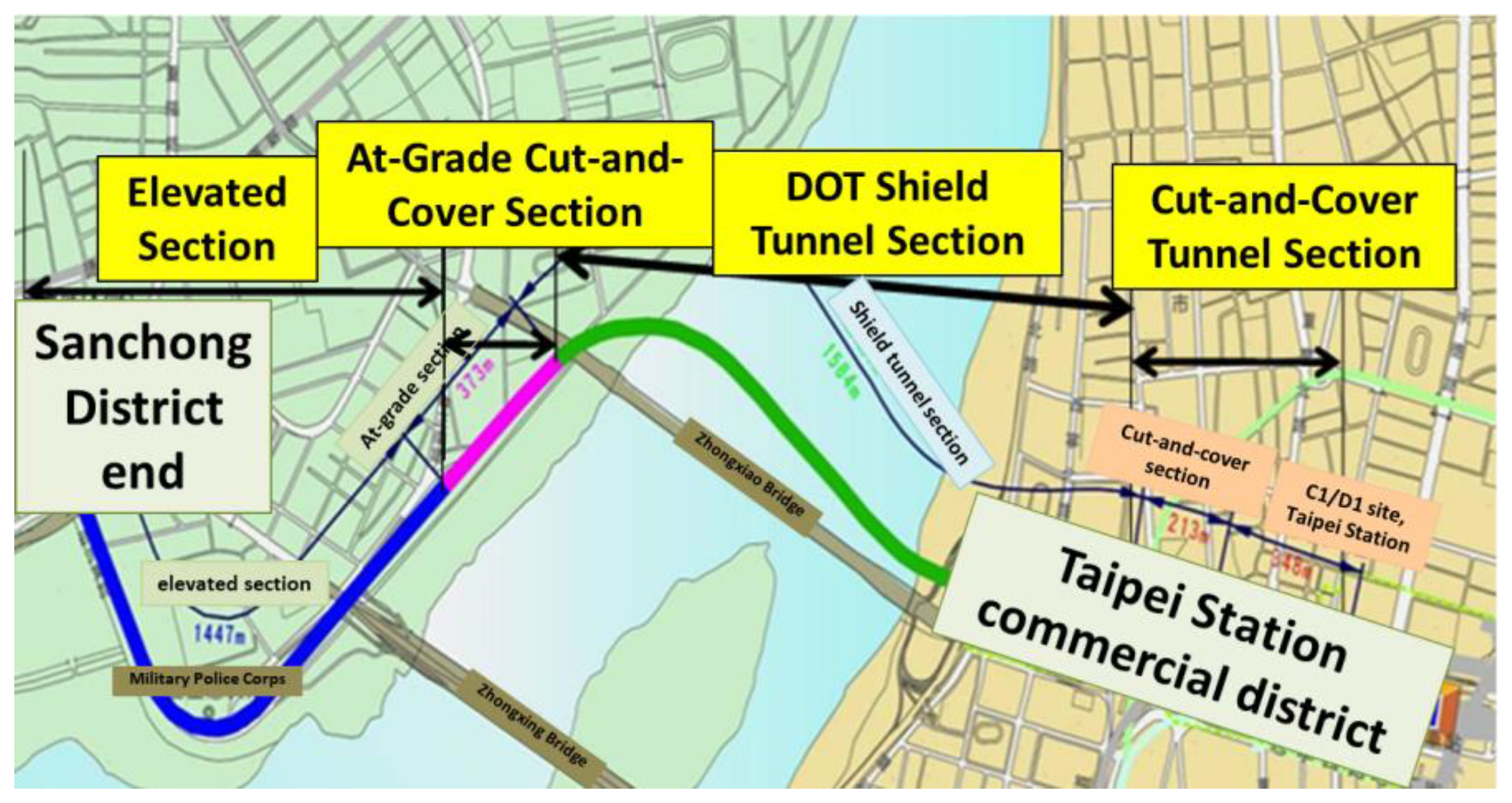
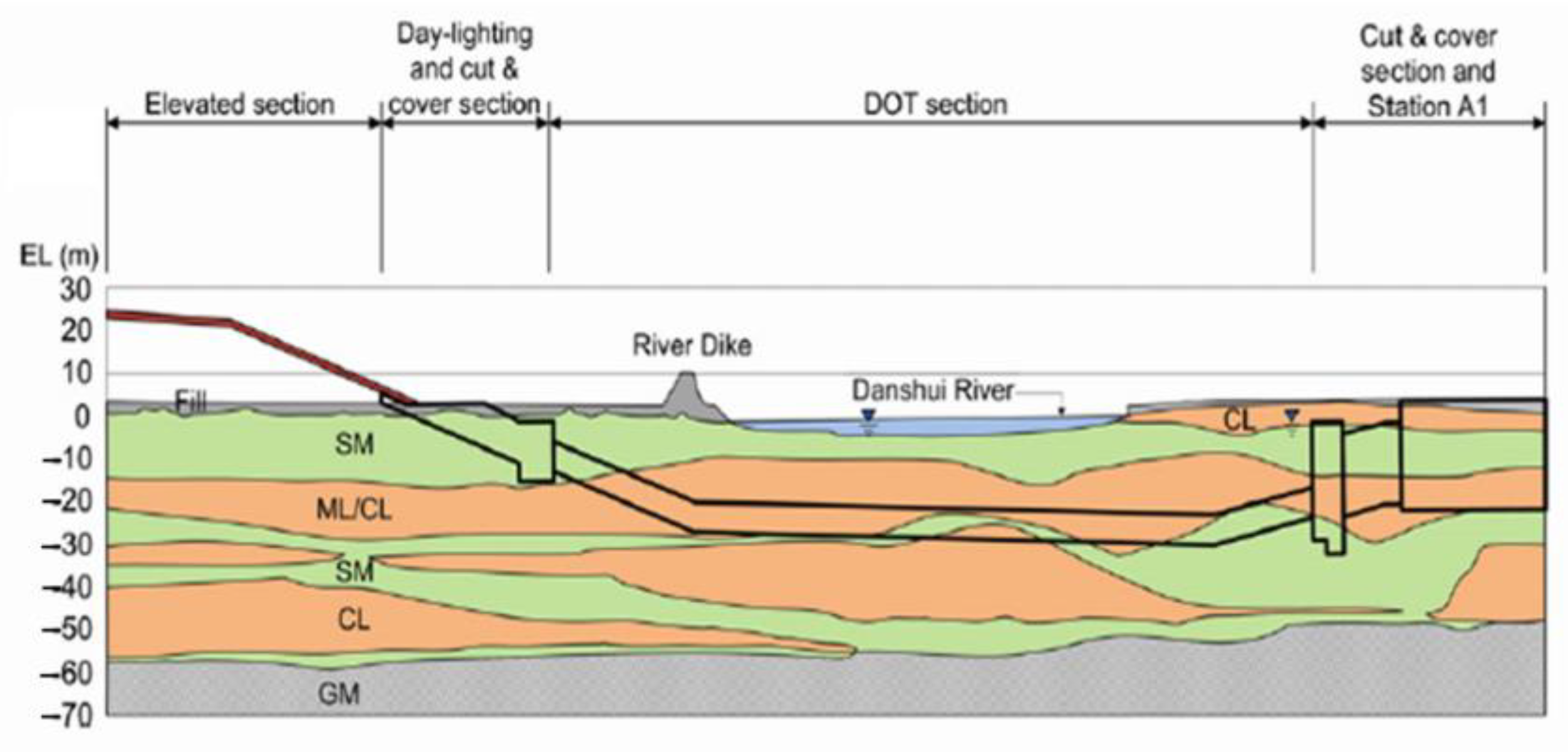
2.2. Case Introduction
3. Numerical Simulation
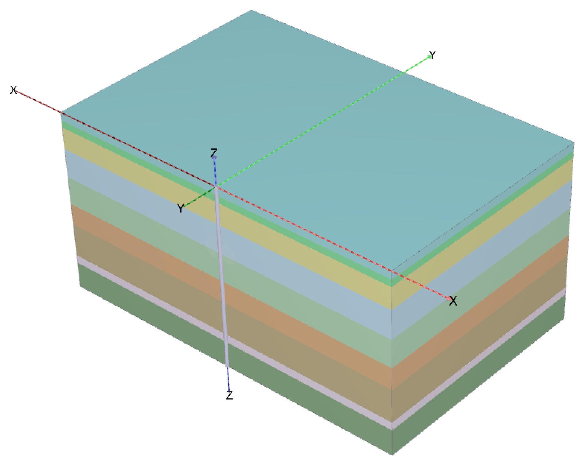
3.1. Model Setup
- -
- Layer 1: Backfill (SF), depth GL 0 to −2.7 m;
- -
- Layer 2: Silty Clay (CL), depth GL −2.7 to −5 m;
- -
- Layer 3: Silty Sand (SM), depth GL −5 to −12.1 m;
- -
- Layer 4: Silty Clay (CL), depth GL −12.1 to −21.5 m;
- -
- Layer 5: Silty Clay (CL), depth GL −21.5 to −30.7 m;
- -
- Layer 6: Silty Sand (SM), depth GL −30.7 to −37.8 m;
- -
- Layer 7: Silty Clay (CL), depth GL −37.8 to −48.8 m;
- -
- Layer 8: Silty Sand (SM), depth GL −48.8 to −51.4 m;
- -
- Layer 9: Silty Gravel (GM), depth GL −51.4 to −60 m.
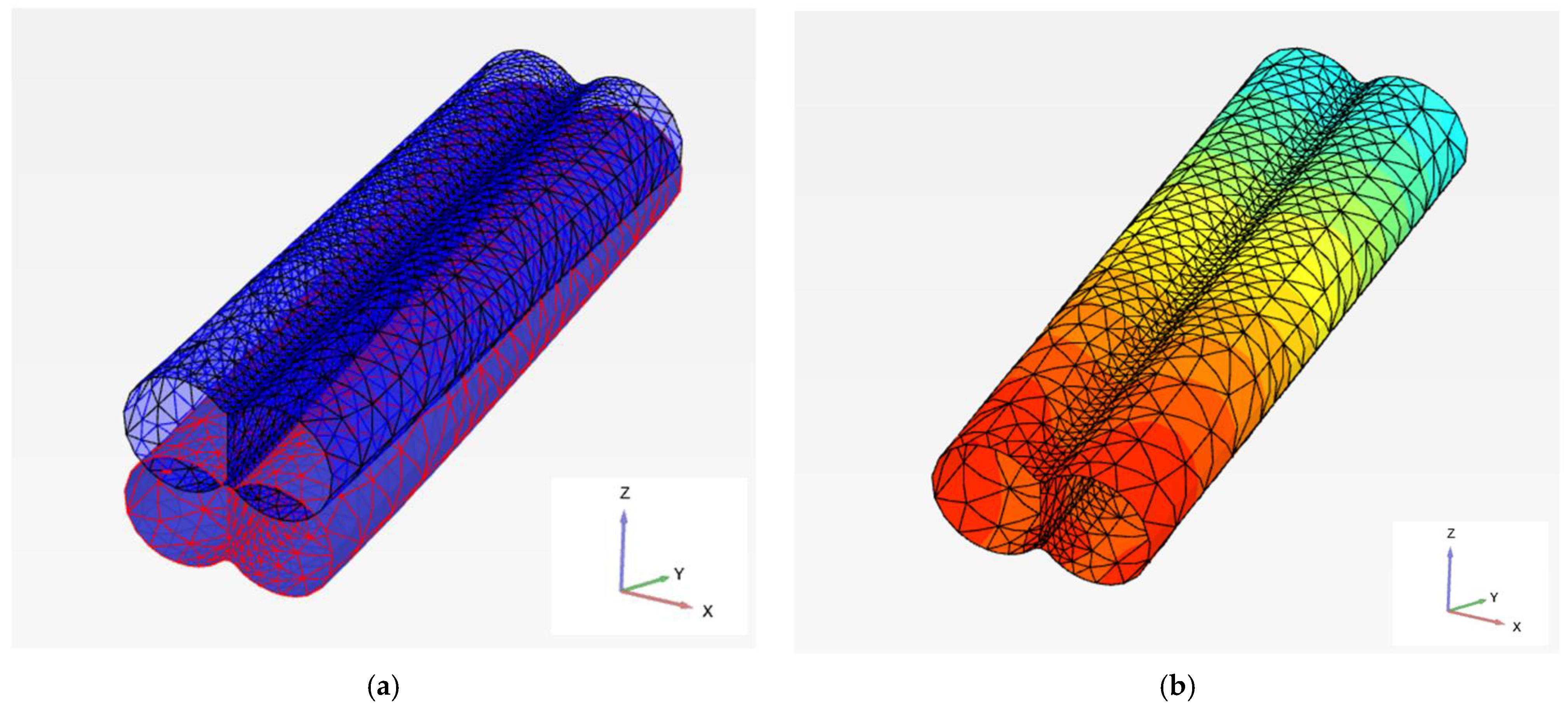
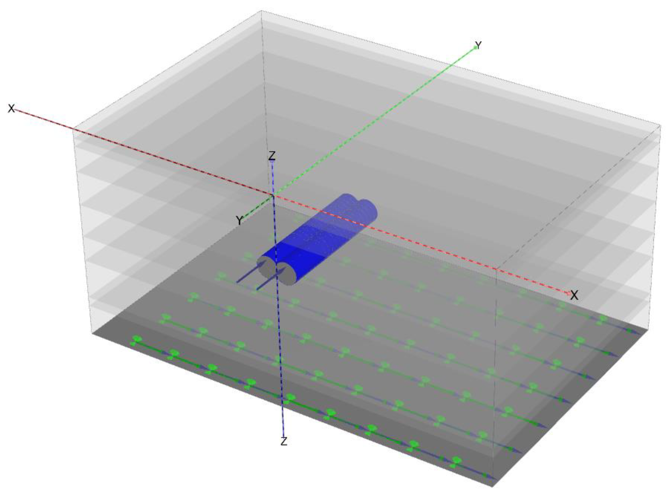
3.2. Tunnel Installation
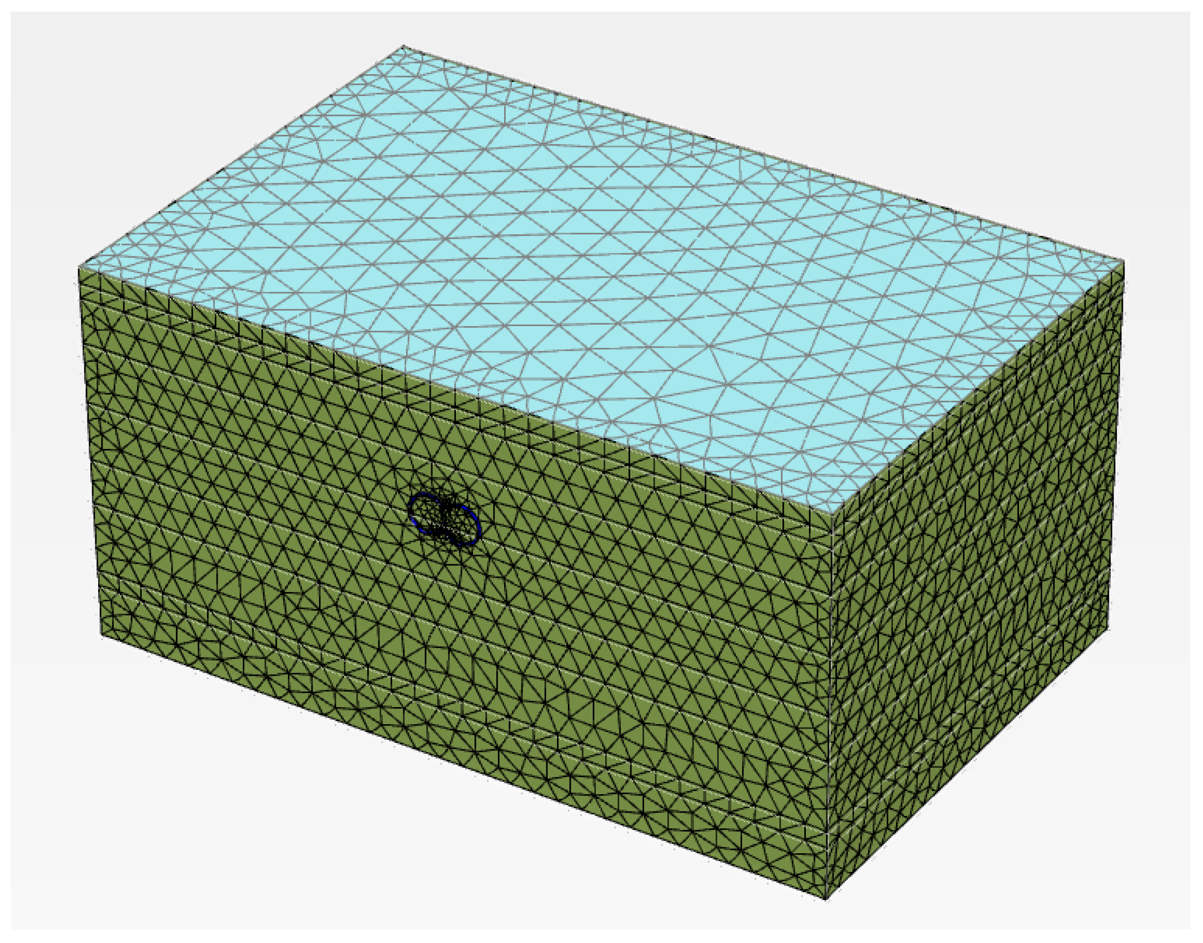
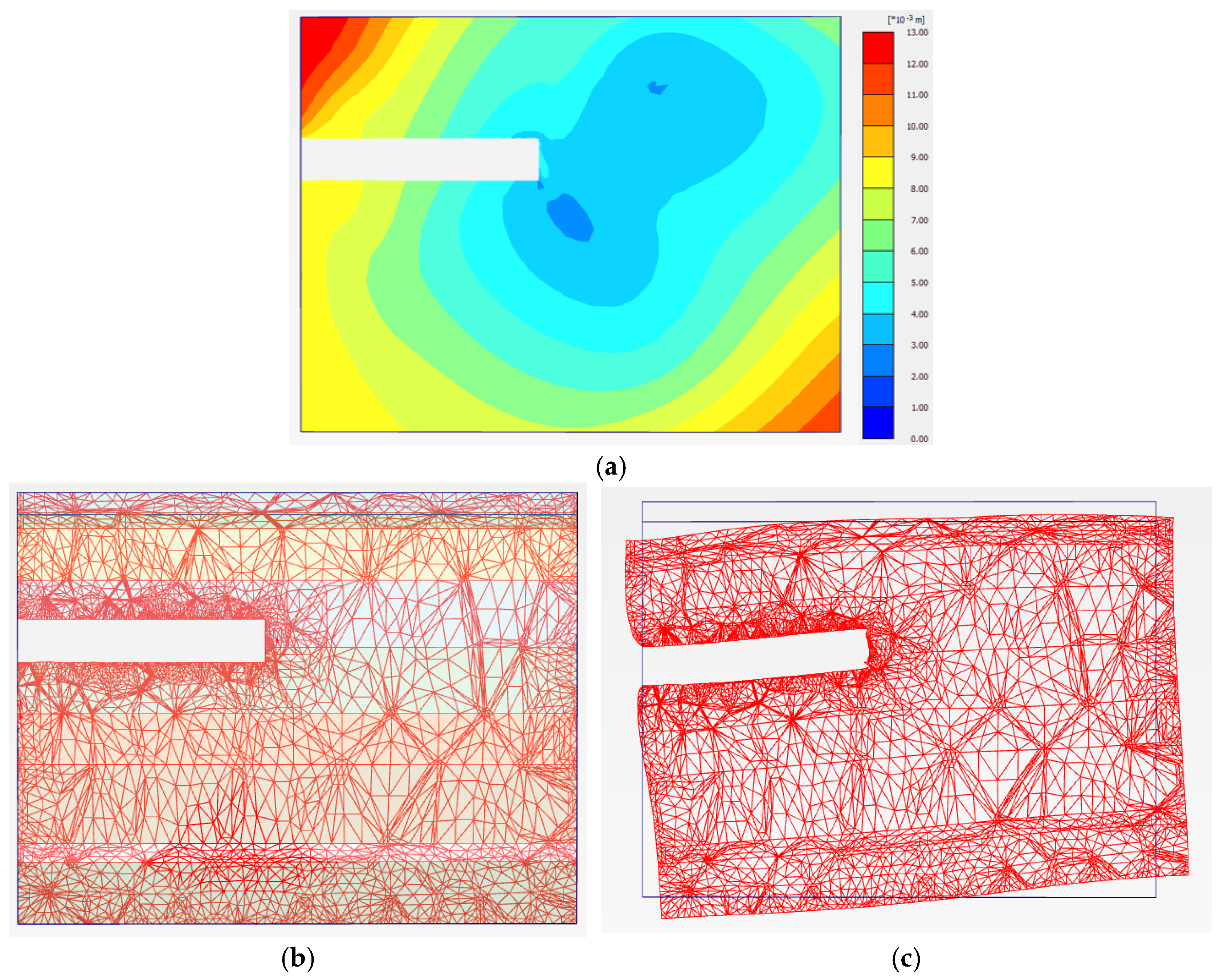
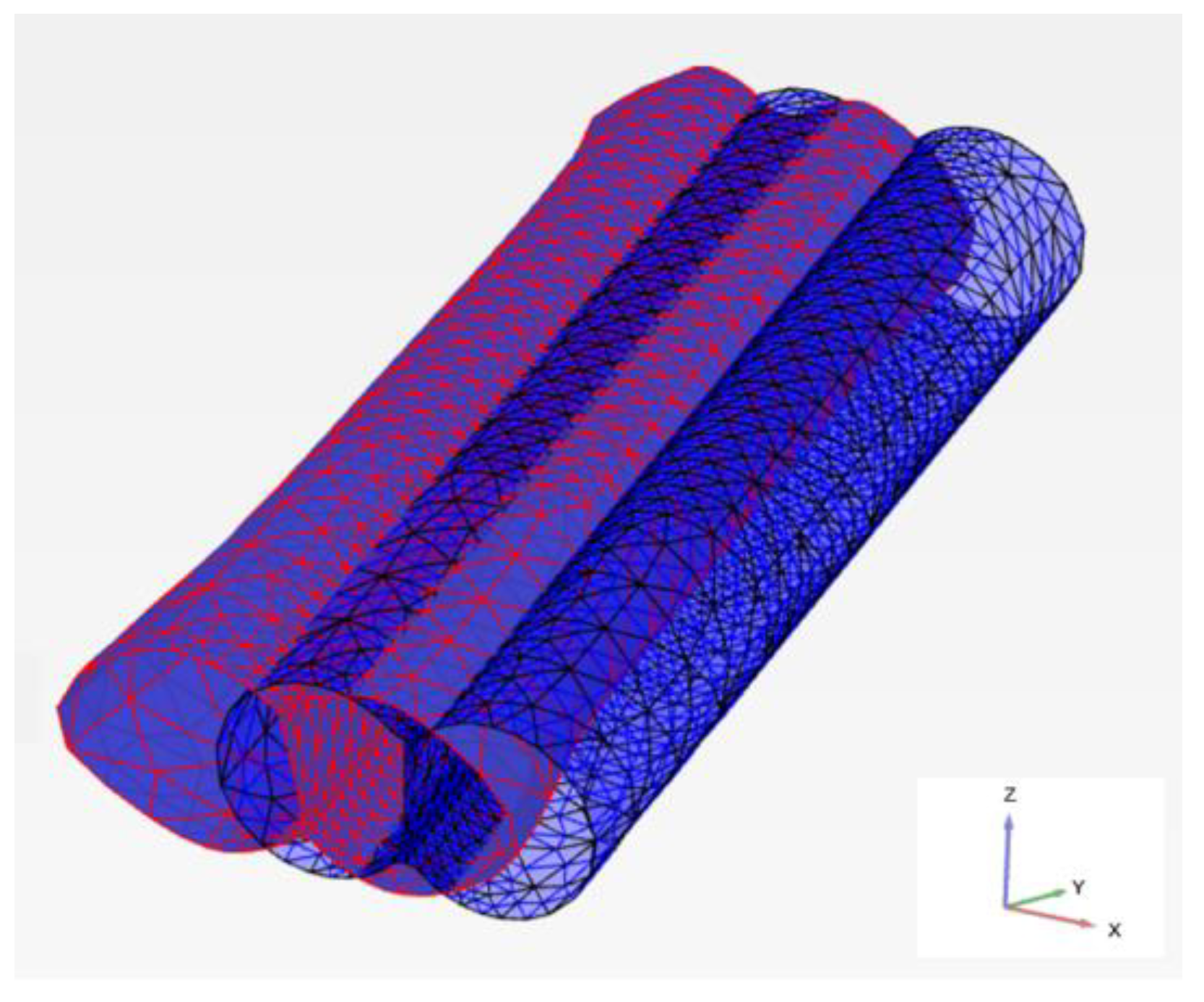
3.3. Mesh Generation
3.4. Seepage Conditions
3.5. Dynamic Boundaries
- Use of semi-infinite elements (boundary elements);
- Adjustment of boundary material properties (low stiffness and high viscosity);
- Application of viscous boundaries (dashpots);
- Use of free-field and compliant boundaries (boundary elements).
3.6. Damping
- −
- M is the mass matrix;
- −
- C is the damping matrix;
- −
- K is the stiffness matrix;
- −
- F is the load vector;
- −
- is acceleration;
- −
- is velocity;
- −
- u is displacement.
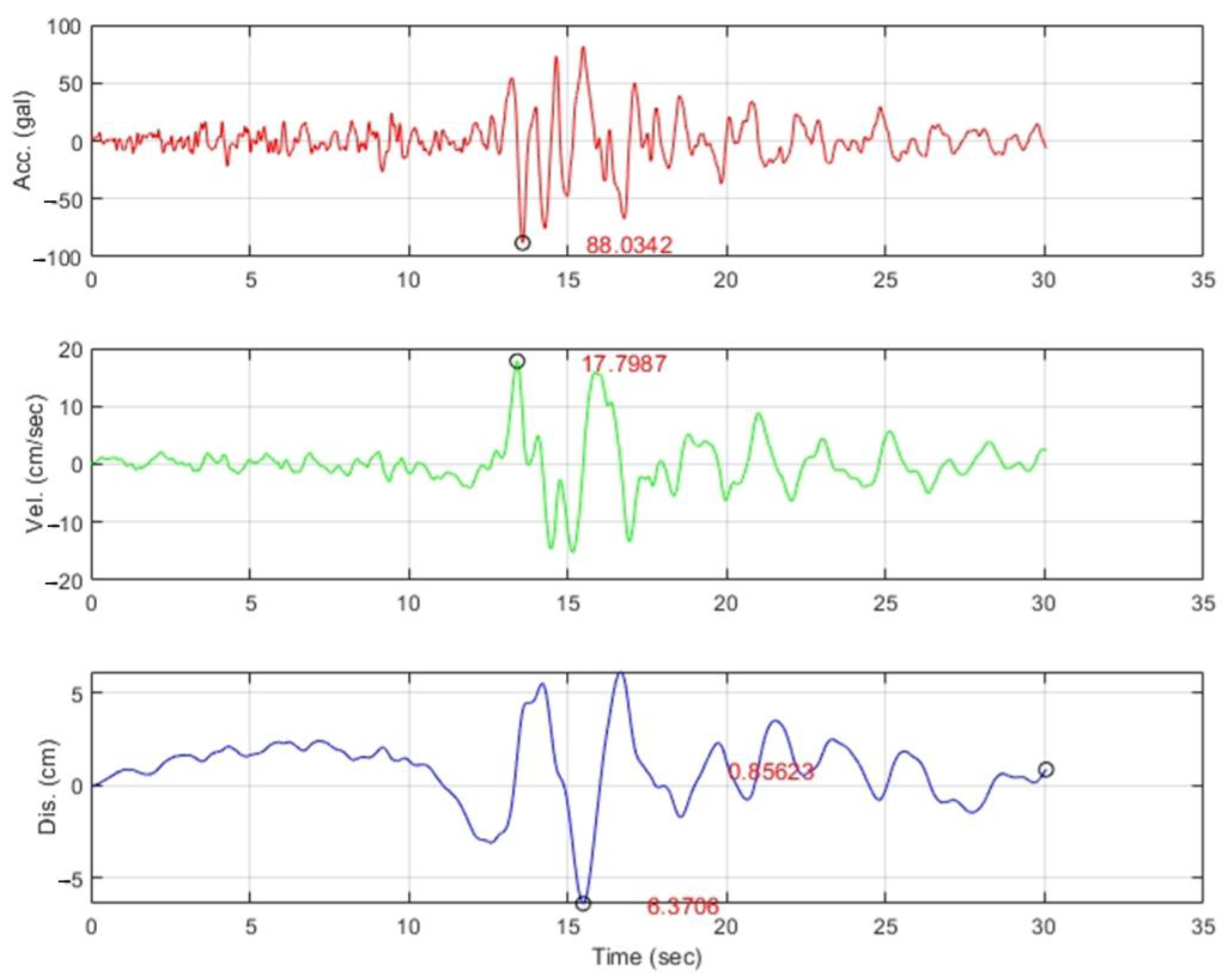
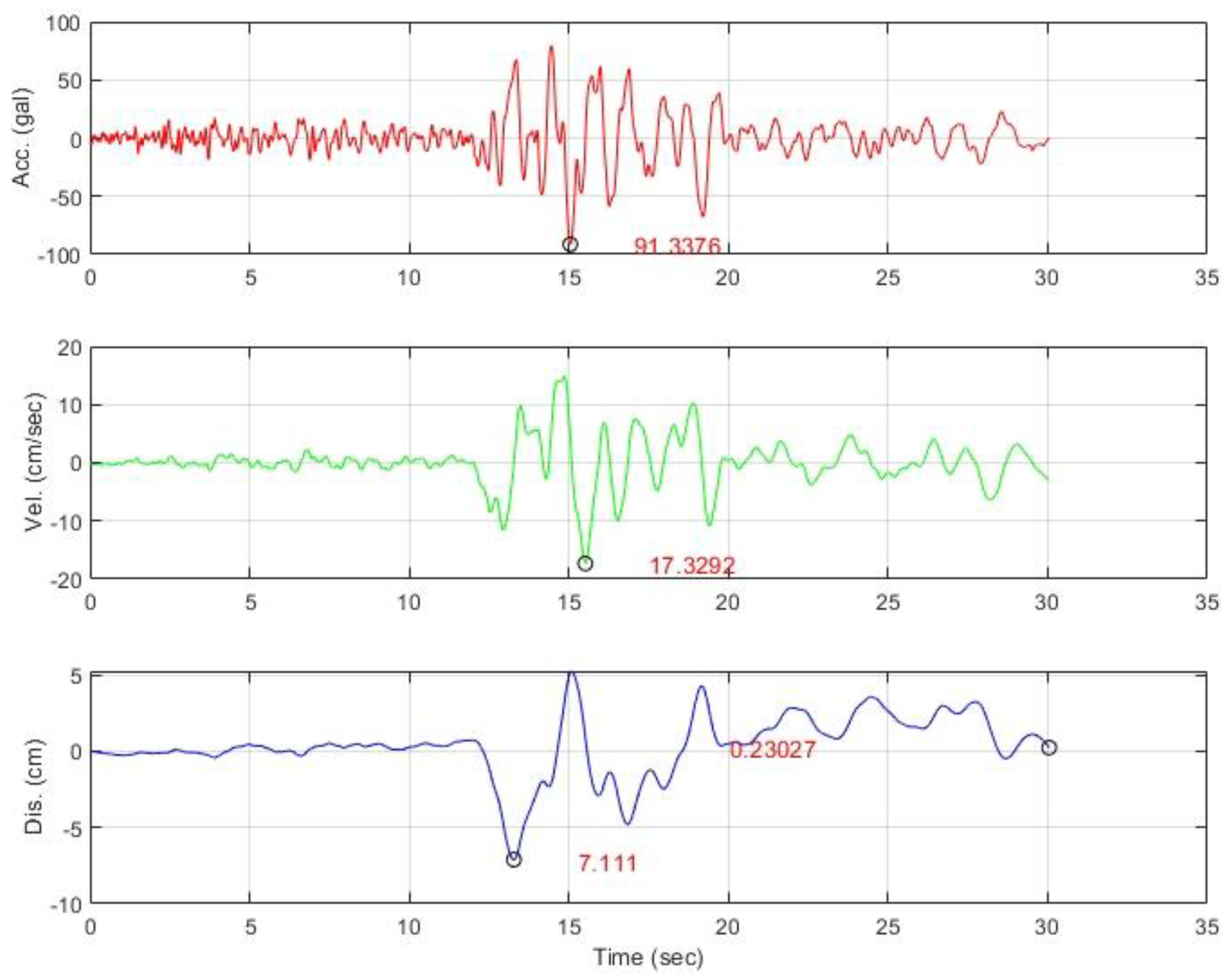
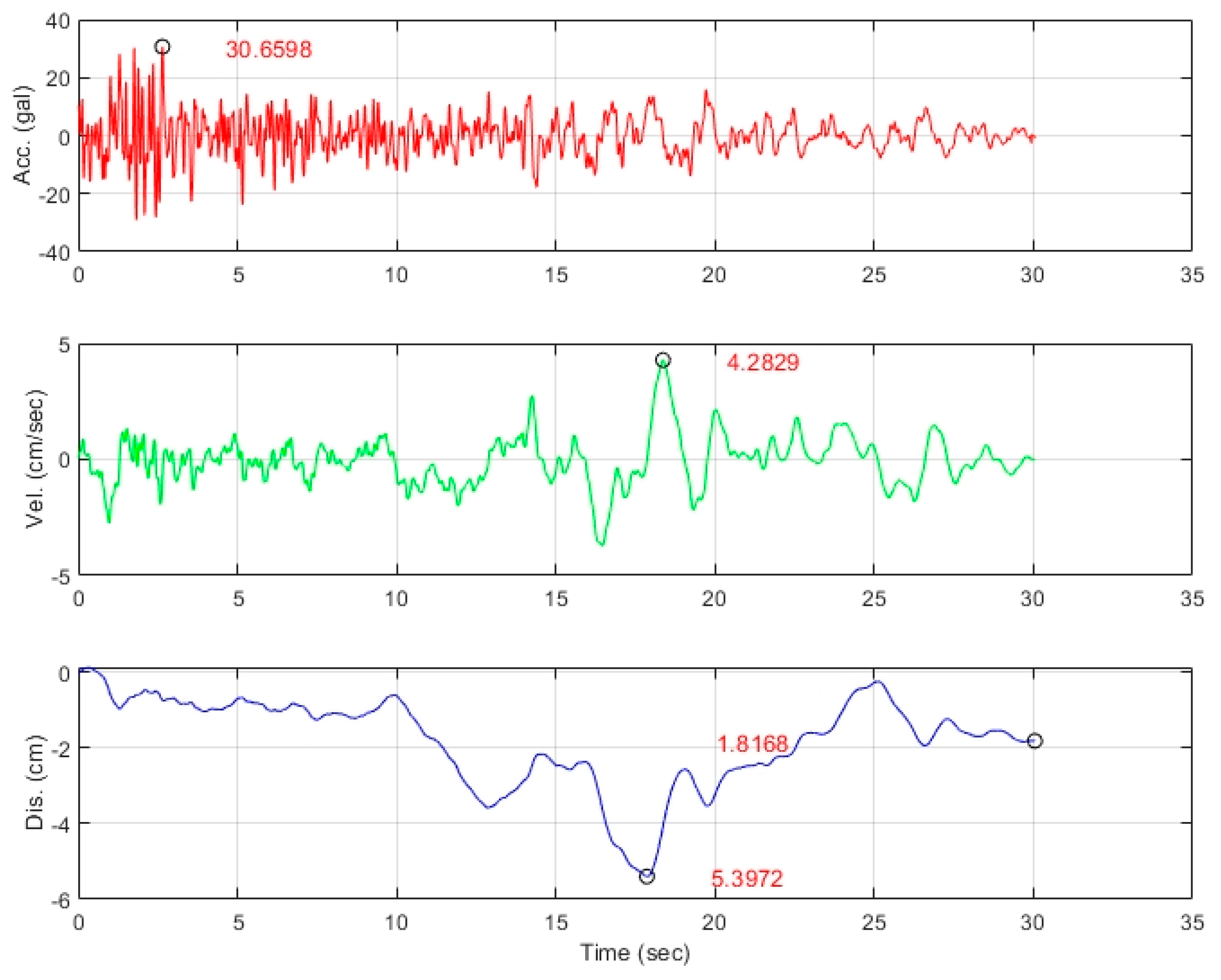
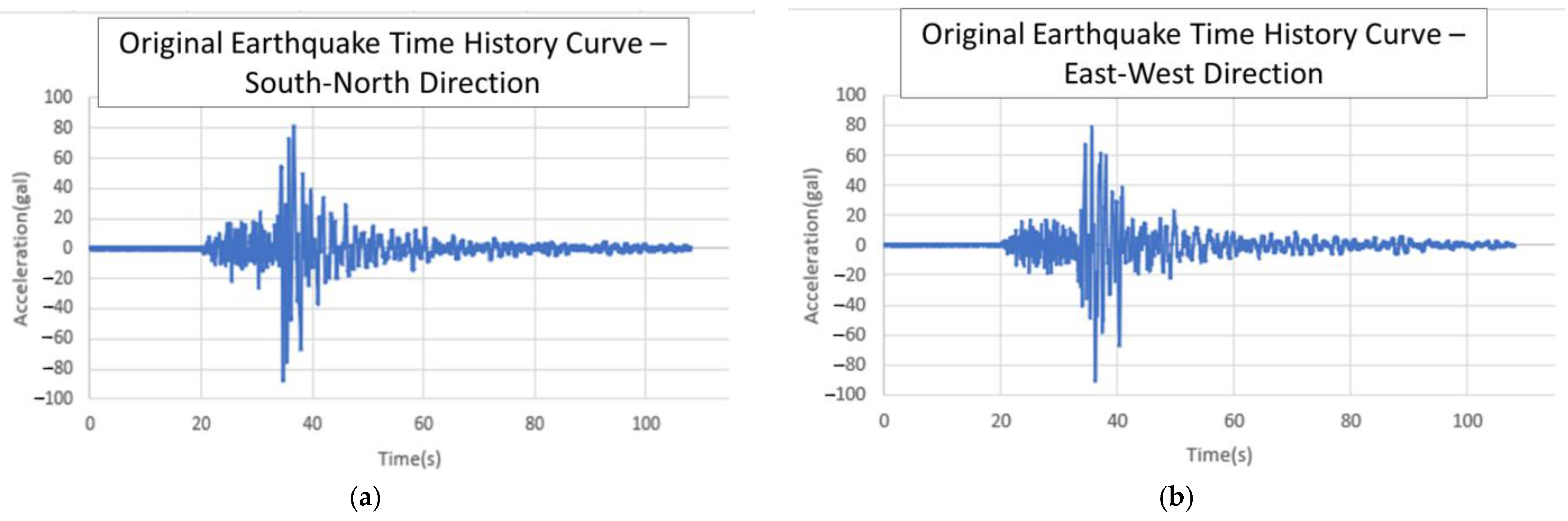
3.7. Earthquake Data
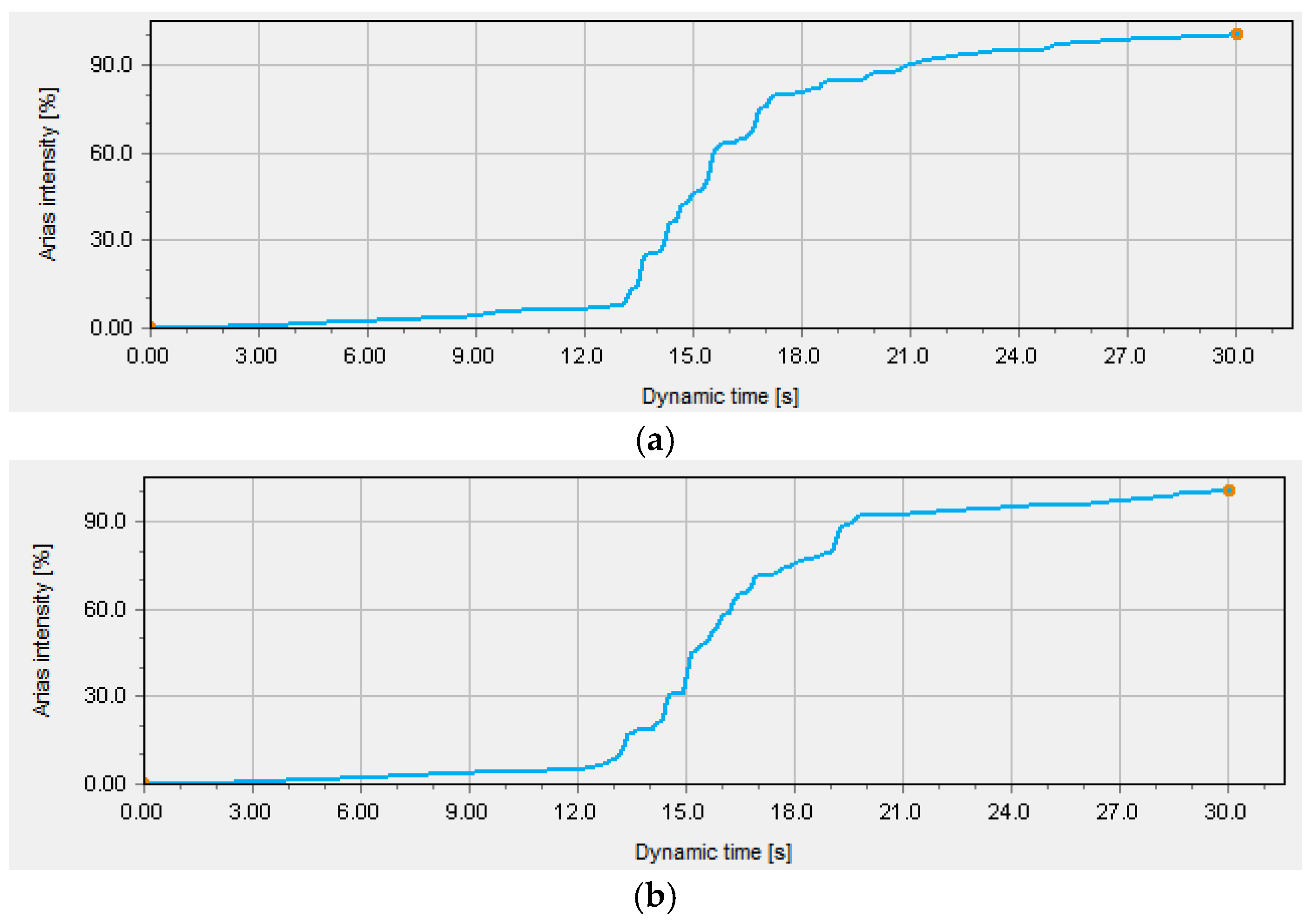
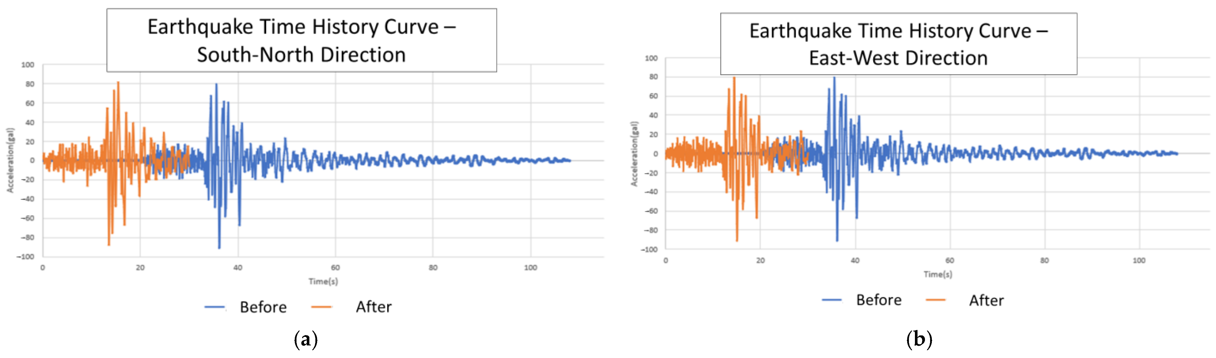
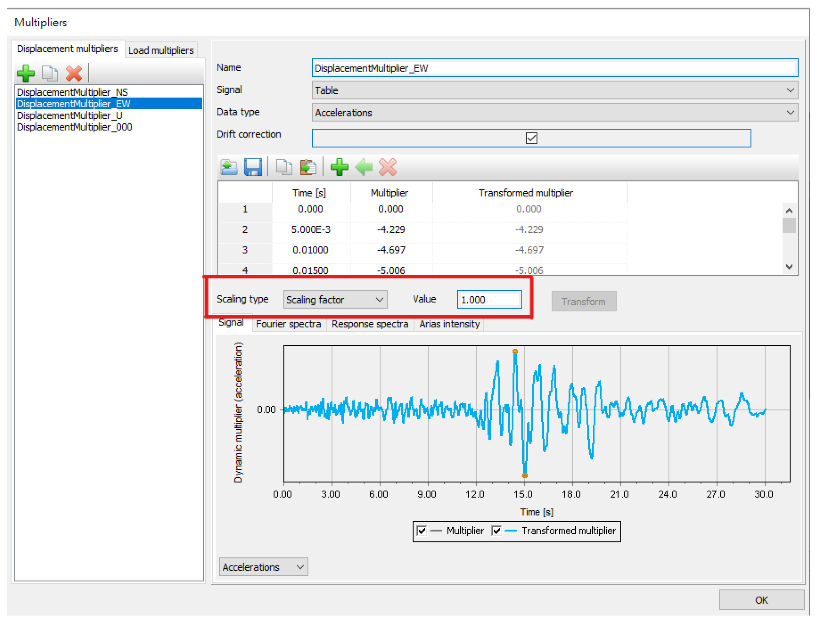
3.8. Ground Motion Scaling
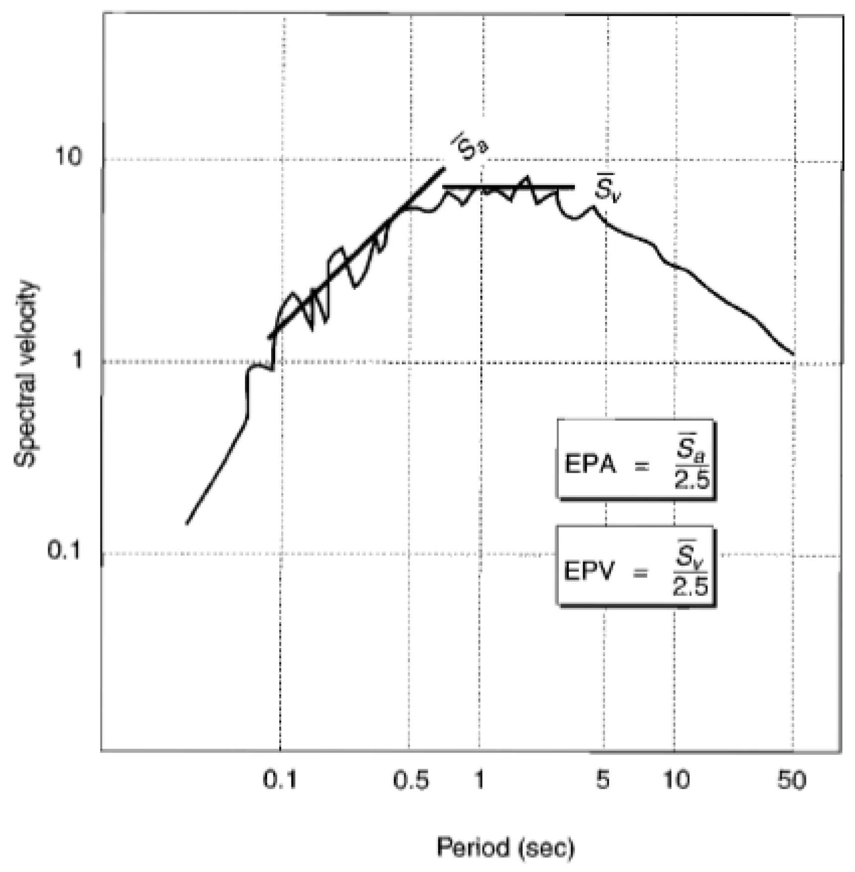
3.9. Seismic Load Amplification
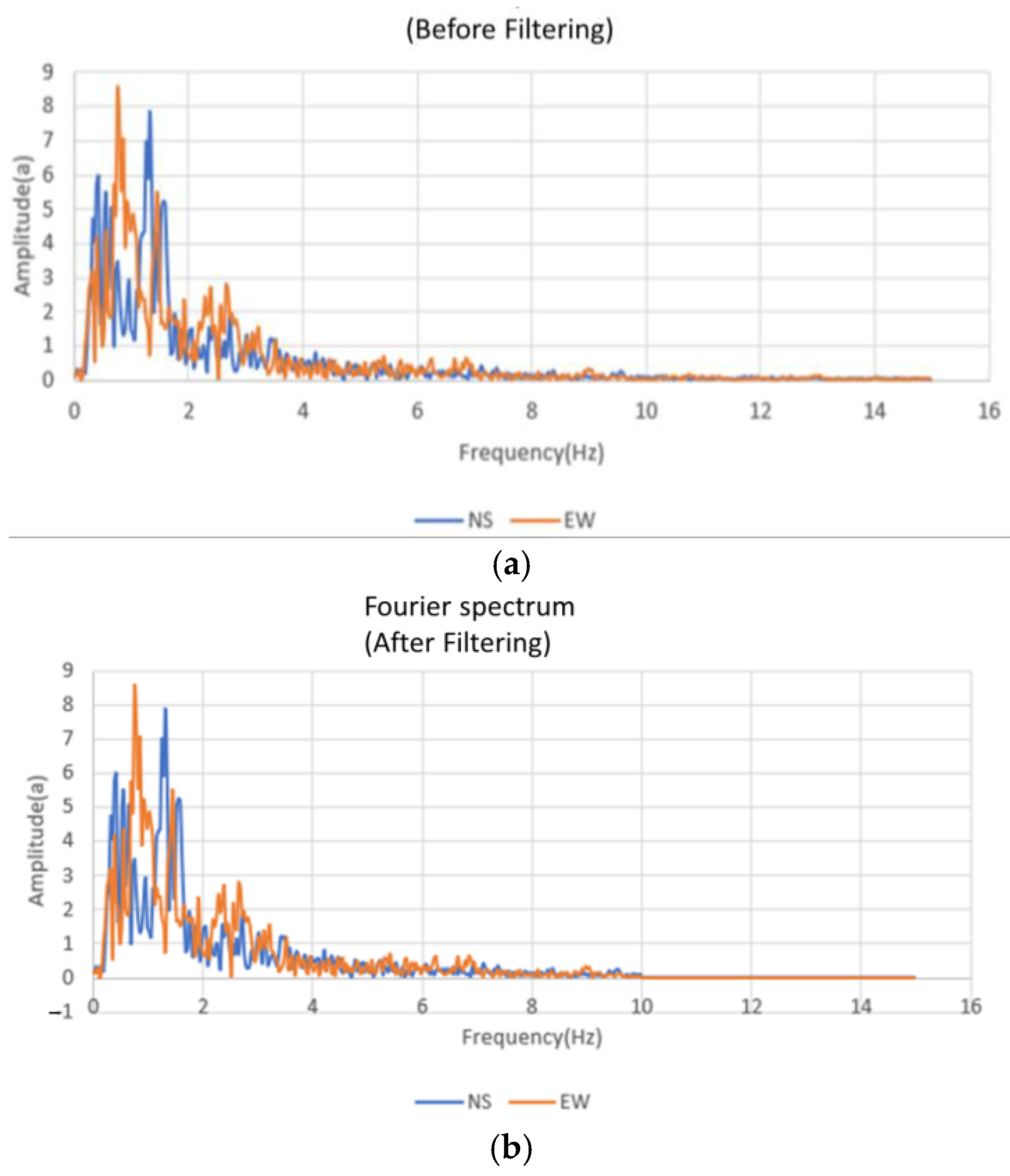
3.10. Baseline Correction
3.11. Calculation and Output Results
4. Discussion
4.1. Influence of Tunnel Excavation on Surface Settlement
- (1)
- Causes of Surface Settlement Induced by Tunnel Excavation
- (2)
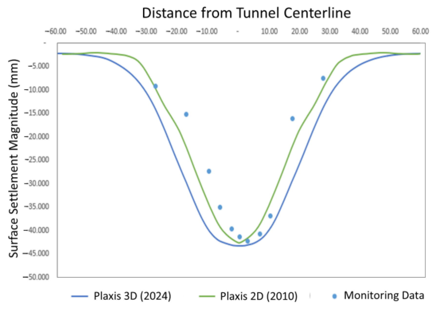
- Comparison of Surface Settlement Results Induced by Tunnel Excavation
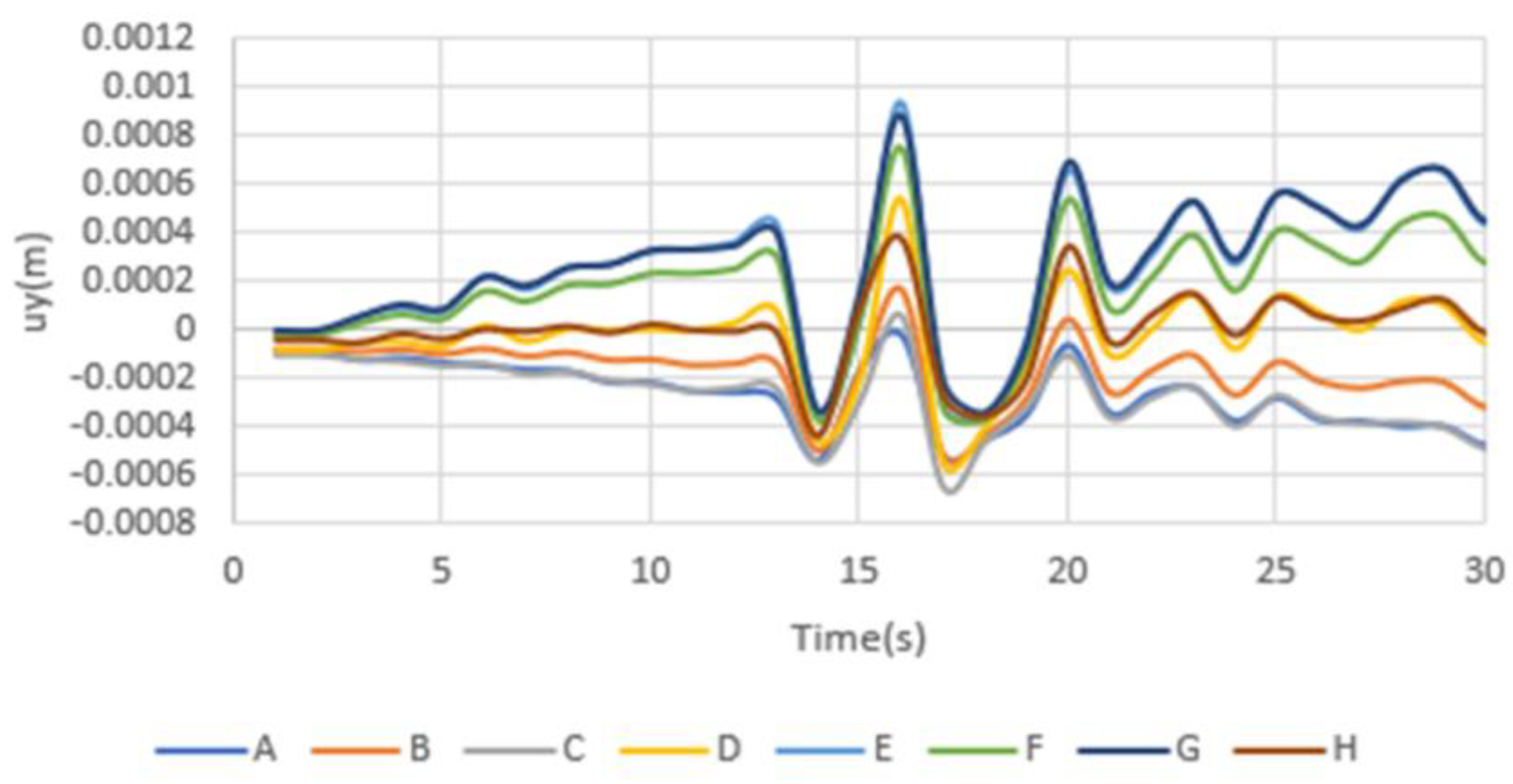
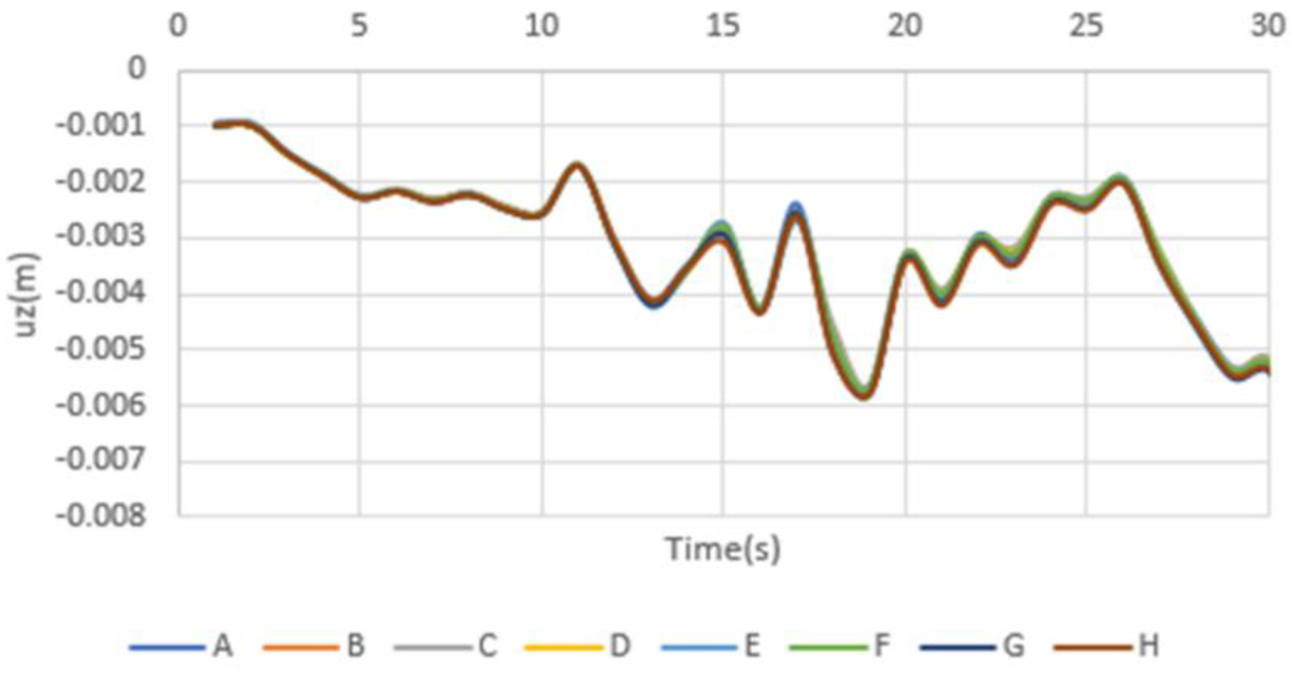
4.2. Displacement Analysis of Tunnel Under Seismic Loading
- (1)
- Soil Deformation
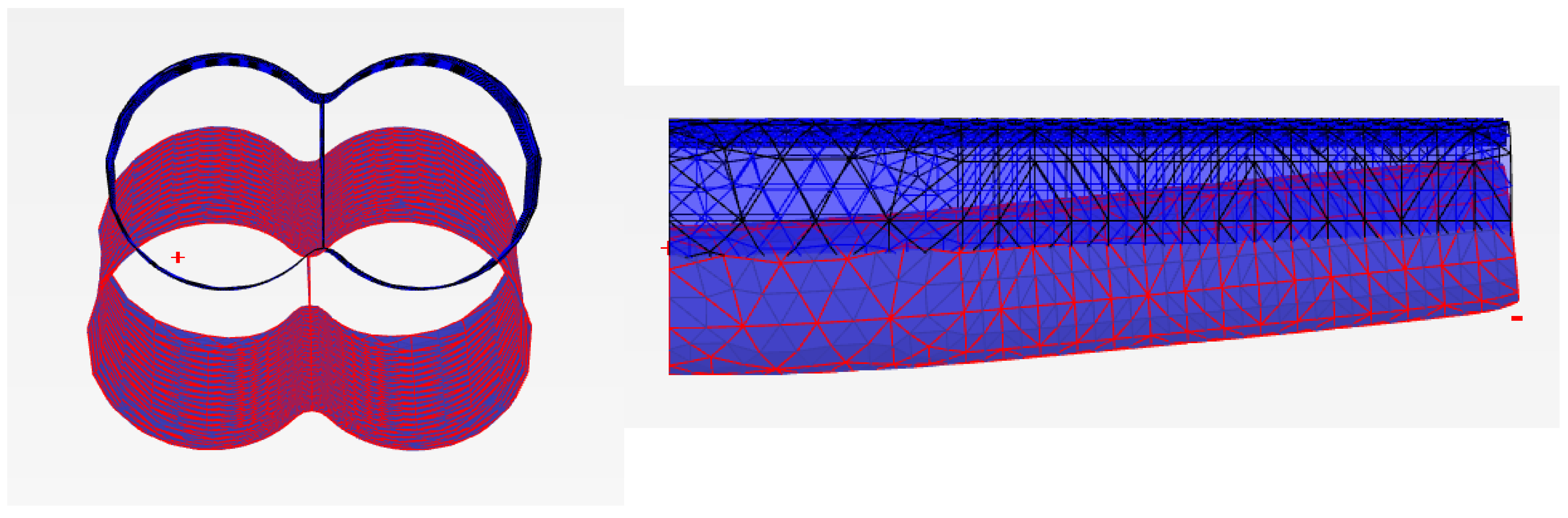
- (2)
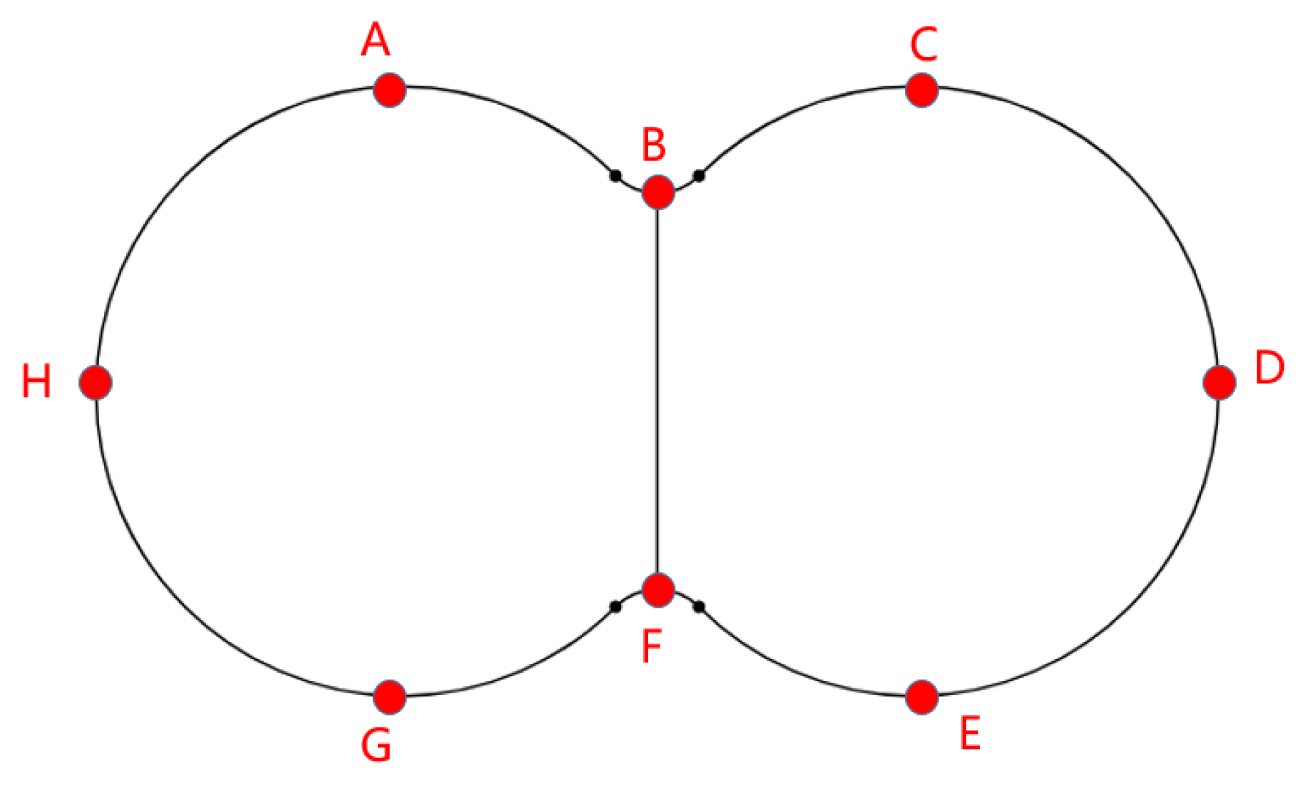
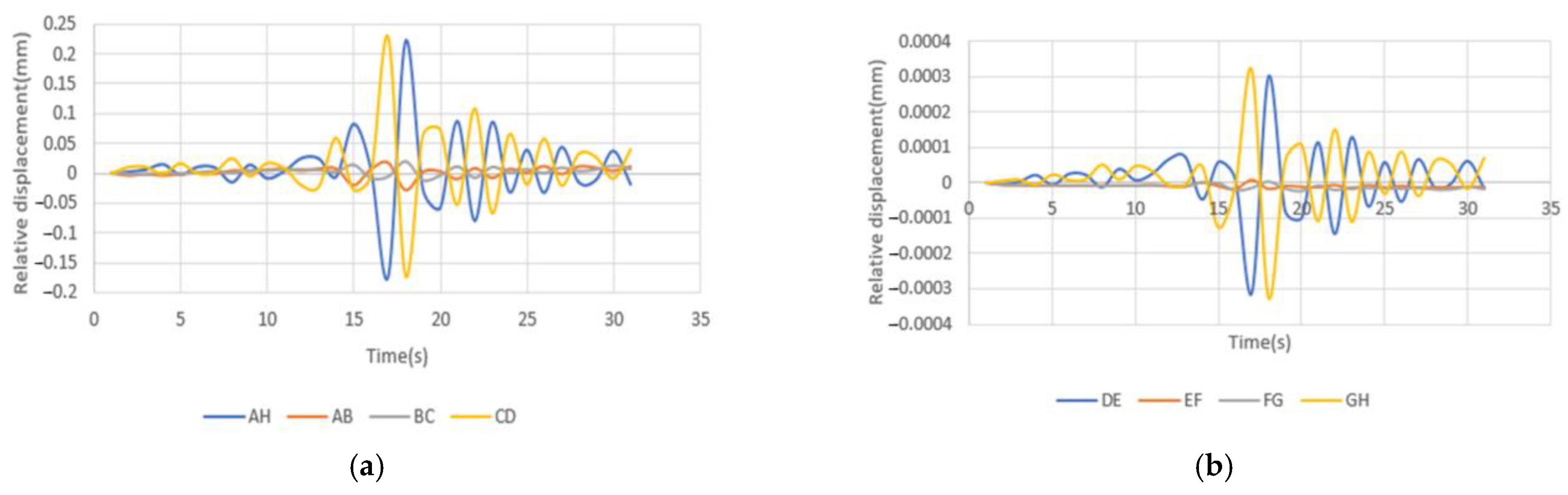
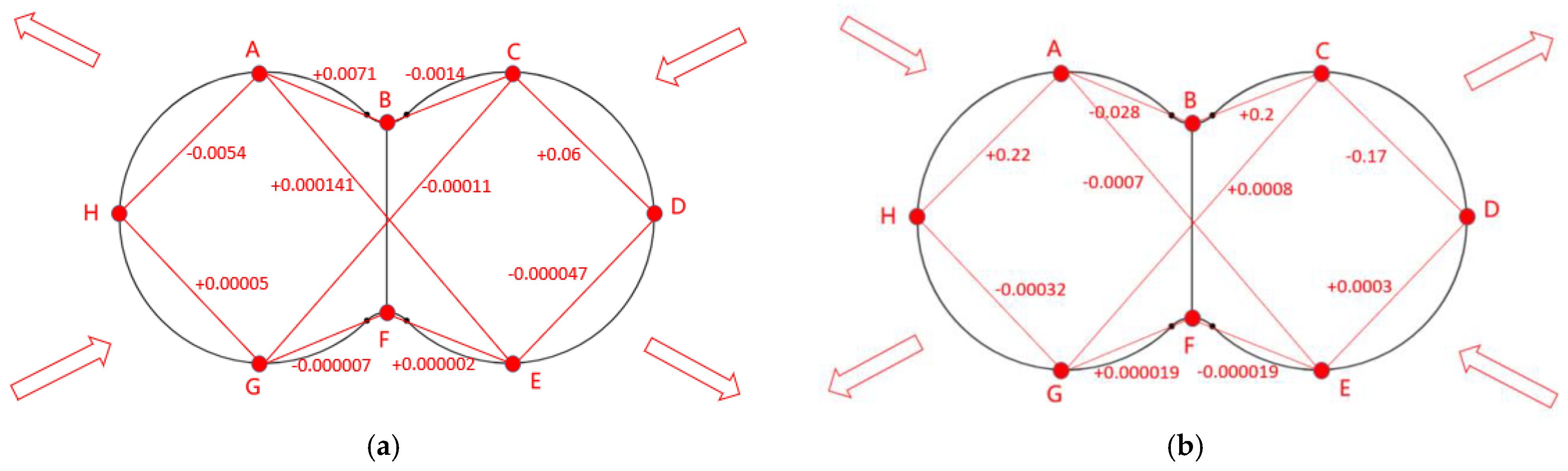
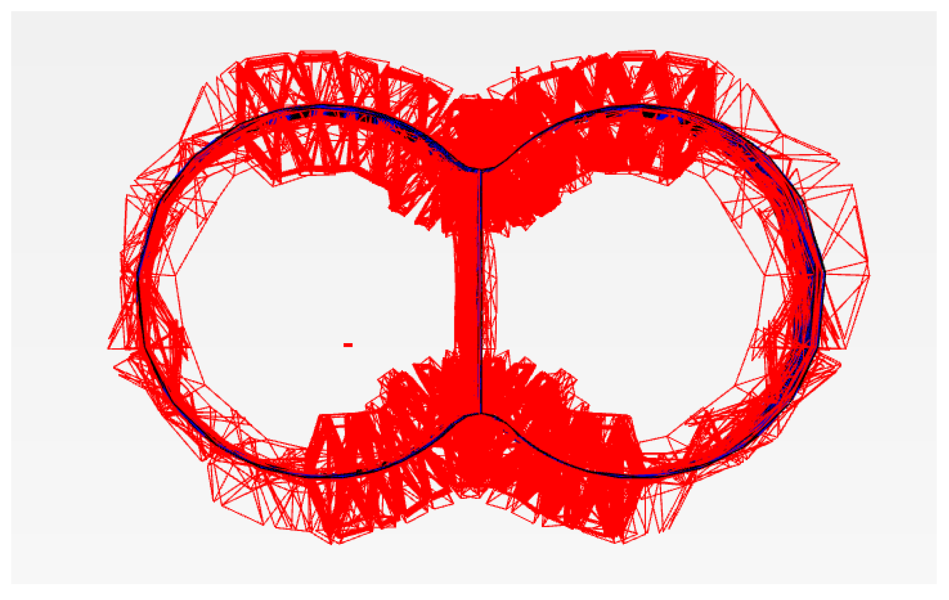
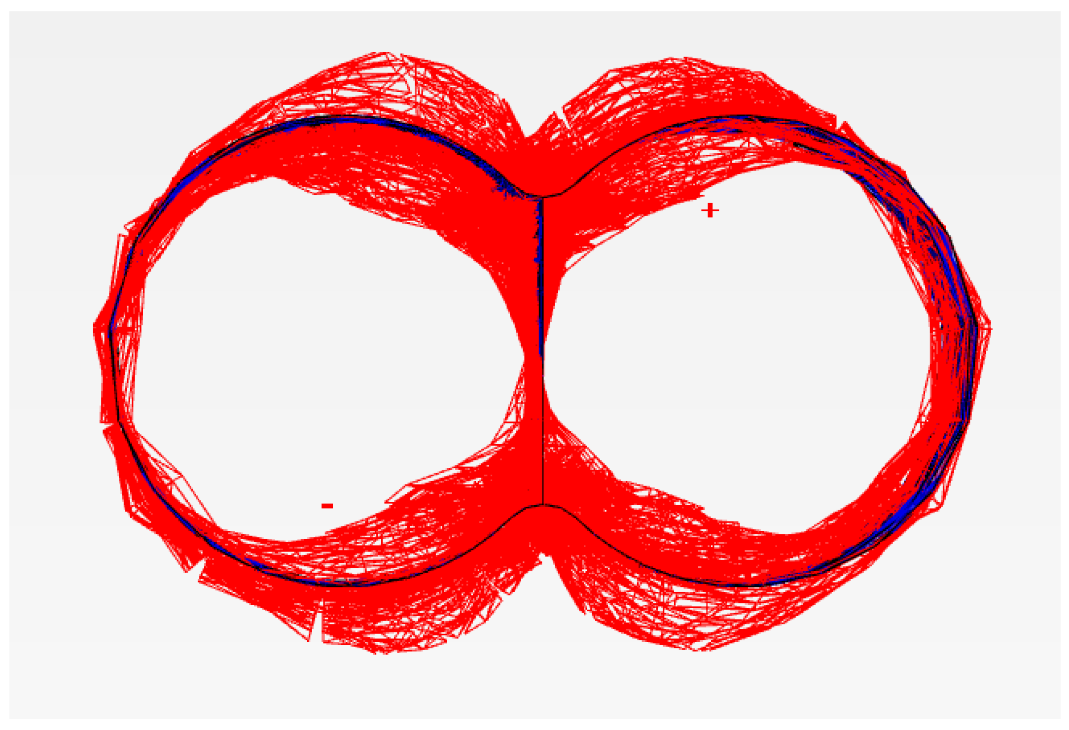
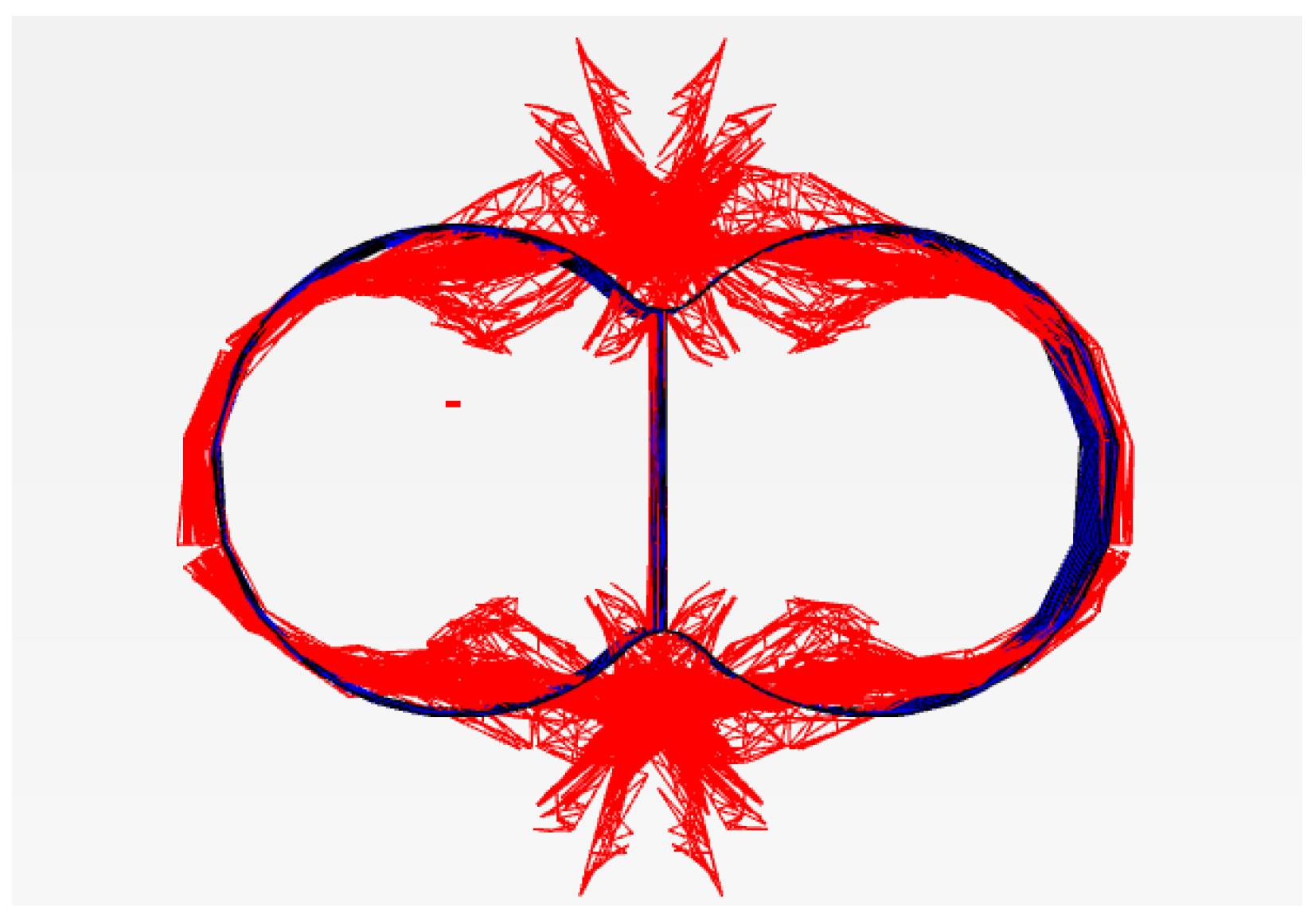
- Tunnel Cross-Section Analysis
4.3. Mechanical Behavior Analysis of Tunnel Under Seismic Loading
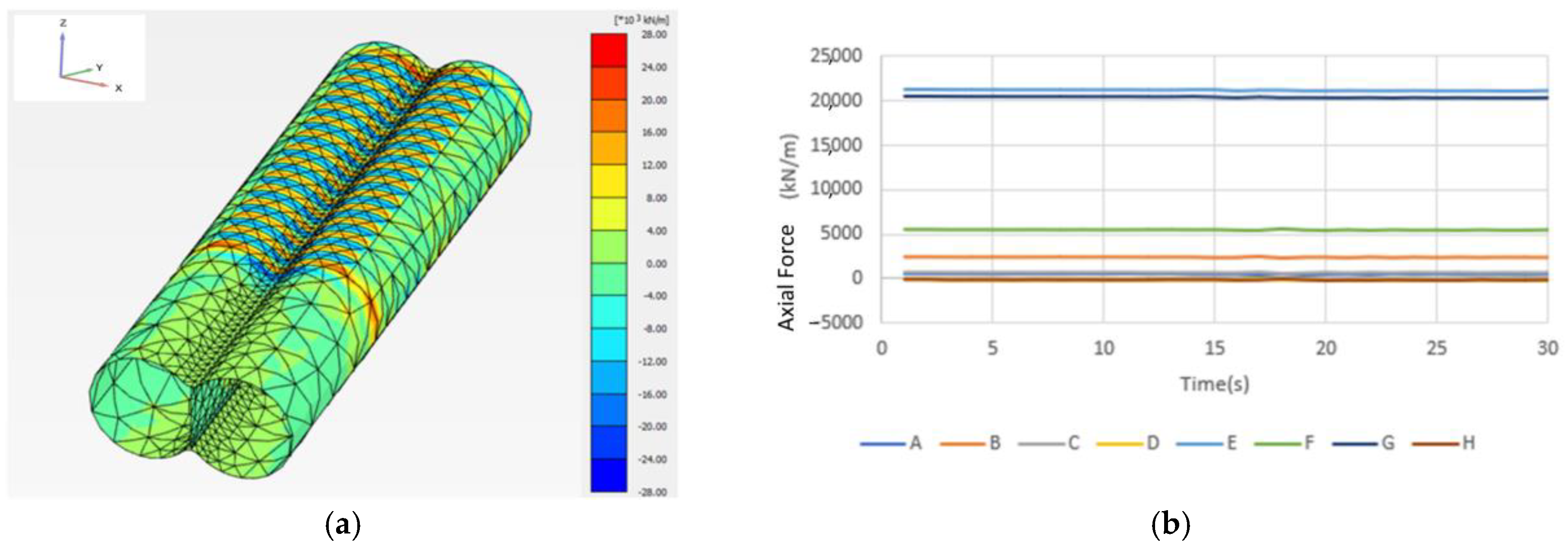
- (1)
- Axial Force Analysis
- (2)
- Shear Force Analysis
- (3)
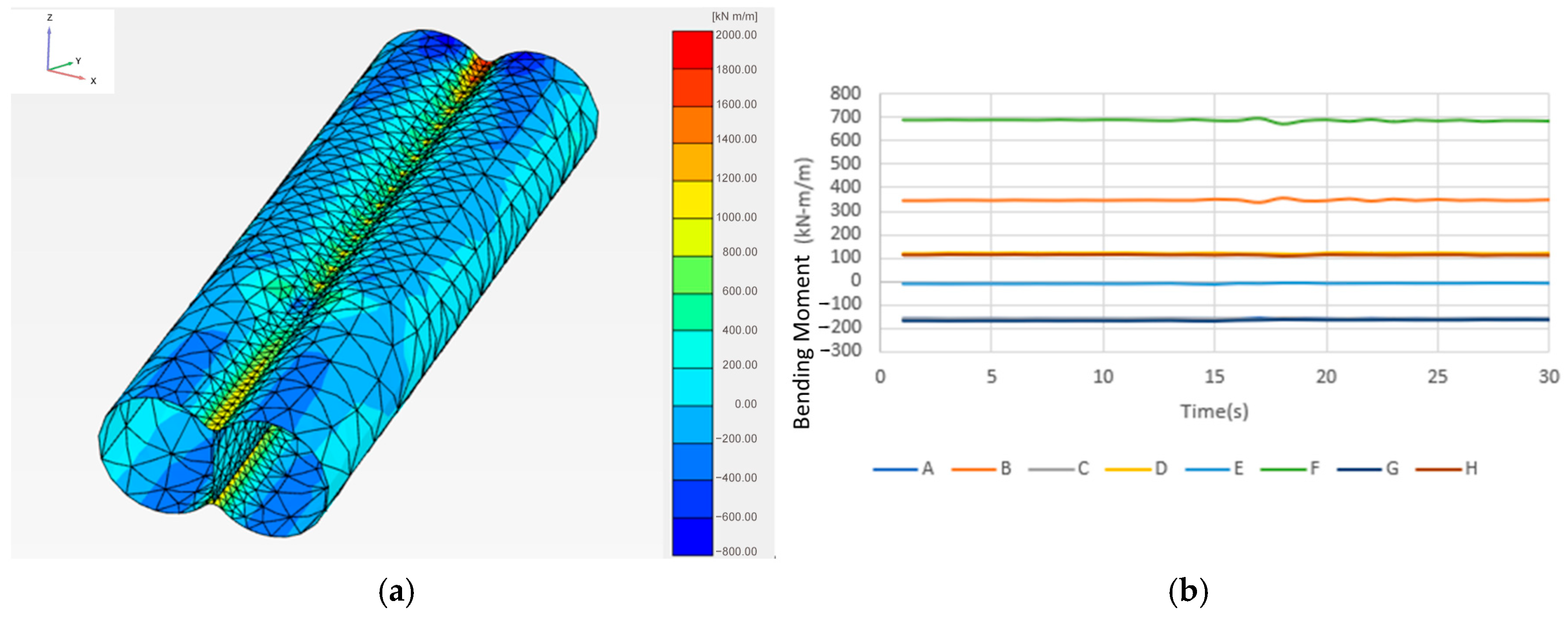
- Bending Moment Analysis
4.4. Mechanical Behavior Analysis of Tunnel Under Earthquakes with Varying Intensities
- (1)
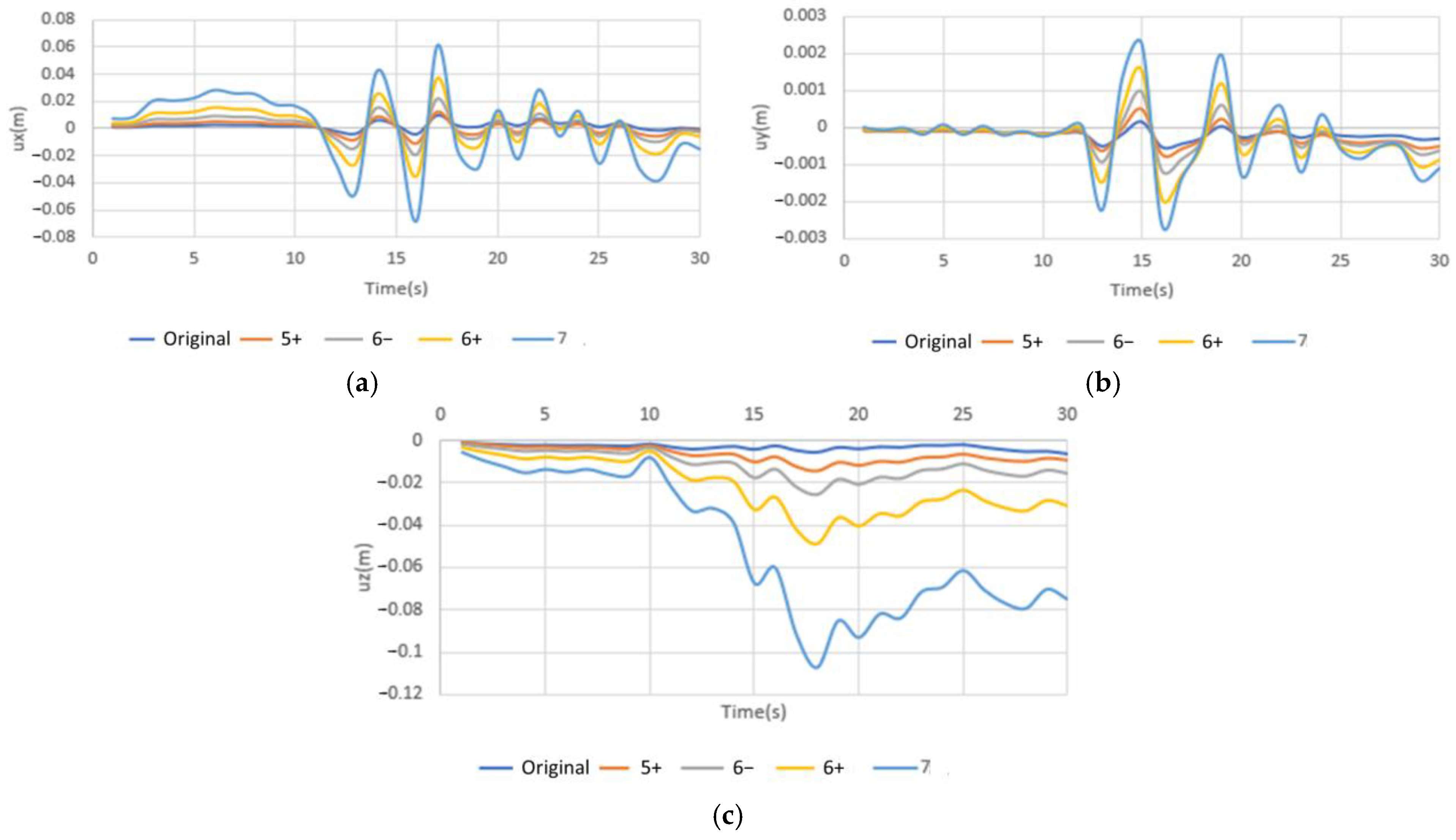
- Displacement Behavior of Tunnel
- -
- X-axis: Displacement increases to ~1.75× (Intensity 5+), 3.05× (6−), 4.9× (6+), and 6.73× (7) of the original.
- -
- Y-axis: Increases to ~2.55×, 5.08×, 8.54×, and 13.27×, respectively.
- -
- Z-axis: Increases to ~1.5×, 2.67×, 5.52×, and 13.2×, respectively.
- (2)
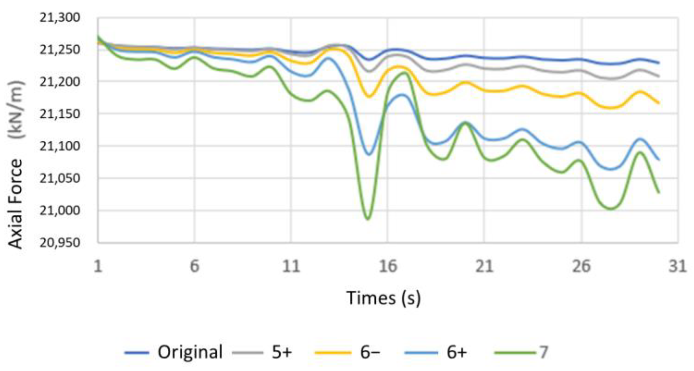
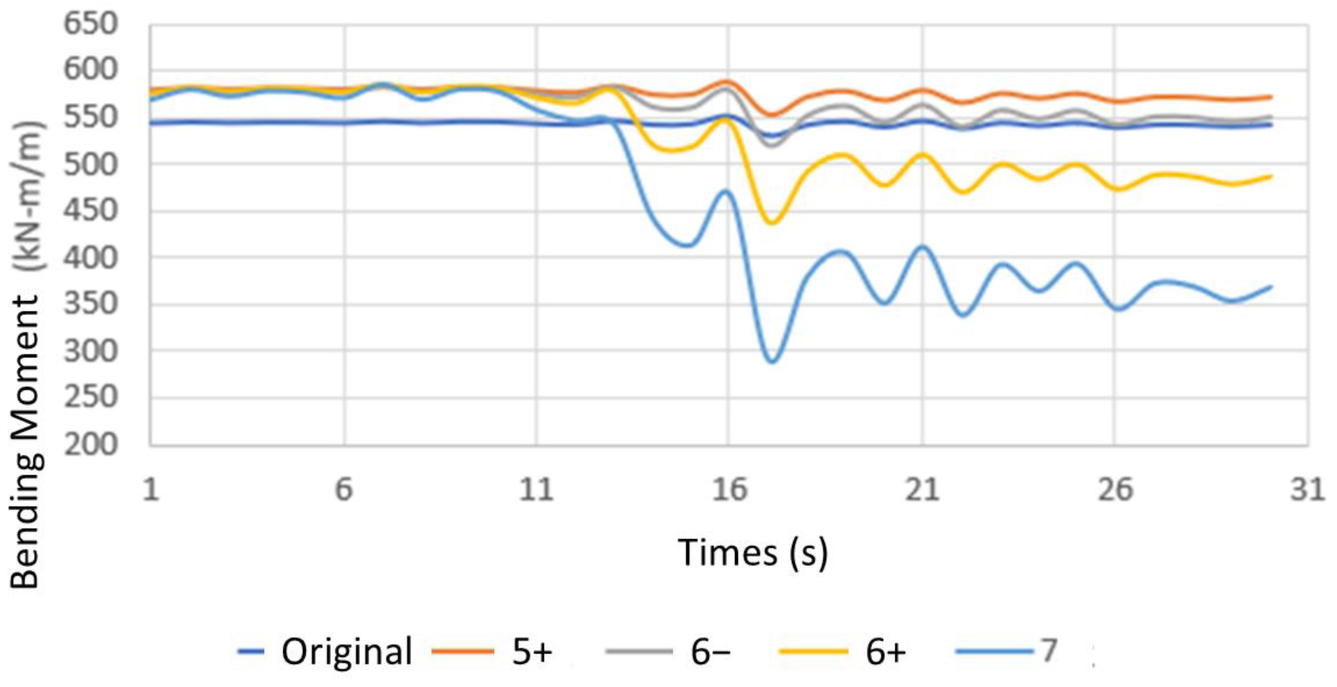
- Changes in Tunnel Mechanical Behavior Under Earthquakes of Varying Intensities
- ▪
- Axial Force Variation at Point E of Tunnel
- ▪
- Shear Force Variation at Point B of Tunnel
- ▪
- Bending Moment Variation at Point F of Tunnel
4.5. Research Limitation
- (1)
- Soil Stiffness Considerations
- (2)
- Modeling Simplification in Plaxis 3D
5. Conclusions
5.1. Summary of Findings
- (1)
- Static analysis: the simulated settlement trough exhibited some deviation from field monitoring data, likely due to model simplifications, such as the use of plate elements for the tunnel lining and central column, and the omission of long-term consolidation effects. However, the predicted maximum settlement was consistent with observed values, indicating reasonable accuracy in capturing localized ground deformation.
- (2)
- Dynamic response characteristics: the dynamic analysis revealed that the highest axial forces occurred at the bottom edge of the tunnel (Points E and G), the greatest shear force at the top of the central column (Point B), and maximum bending moments at both the top and bottom of the column (Points B and F). These results highlight the critical role of the central support structure during seismic loading.
- (3)
- Displacement patterns: the tunnel experienced significant displacement in both the vertical and north–south directions, with peak values reaching approximately 0.7 cm and 1.0 cm, respectively. The upper portion of the tunnel moved in the negative direction, while the lower portion moved in the positive direction, consistent with the development of a positive bending moment.
- (4)
- Soil stiffness considerations: the same Young’s modulus was used in both static and dynamic analyses. Since dynamic loading conditions typically result in higher soil stiffness, this assumption may have led to overestimated displacements in the dynamic simulations.
5.2. Recommendations
- (1)
- Reinforcement of central support structures: as seismic forces were concentrated around the top and bottom of the central column, enhanced reinforcement and structural detailing in this area are recommended to improve seismic performance.
- (2)
- Consideration of displacement direction and bending behavior: the simulation revealed opposite directional displacements in the upper and lower tunnel sections, indicating significant bending effects. Segmental lining and joints should be designed to accommodate rotational and differential deformations.
- (3)
- Use of dynamic soil stiffness parameters: since soil exhibits higher stiffness under dynamic loading, it is recommended to increase the Young’s modulus by a factor of 2–3 or apply strain-dependent modulus adjustments to avoid overestimation of seismic displacements.
- (4)
- Improved soil–structure interaction modeling: to enhance the accuracy of settlement prediction, future models should consider using solid elements for tunnel linings and central columns, as well as include long-term consolidation effects.
- (5)
- Standardization of seismic input processing: frequency filtering, Arias intensity matching, and baseline correction have a significant impact on simulation outcomes. Establishing standardized preprocessing procedures is essential for improving model reliability and consistency.
Author Contributions
Funding
Data Availability Statement
Conflicts of Interest
Abbreviations
| DOT | Double-O-Tube |
| EPA | Effective Peak Acceleration |
| EPV | Effective Peak Velocity |
| FEM | Finite Element Method |
| HS | Hardening Soil |
| MRAM | Modified Response Acceleration Method |
| PGA | Peak Ground Acceleration |
| RD | Relative Displacement |
| SSM | Small Strain Model |
Appendix A

| X | Y | Z | |
|---|---|---|---|
| A | −2.7 | 17.25 | −17.49 |
| B | 0 | 17 | −18.57 |
| C | 2.7 | 17.25 | −17.49 |
| D | 5.7 | 17.25 | −20.26 |
| E | 2.47 | 16.84 | −23.68 |
| F | 0 | 17 | −22.6 |
| G | −2.47 | 16.84 | −23.68 |
| H | −5.7 | 17.25 | −20.26 |
Appendix B

References
- Ke, W.-Y. Investigation of Ground Settlement Analysis for Double-O-Tube Shield Tunnel—A Case Study of the Taipei-Sanchong Section of the Airport MRT Line; National Taipei University of Technology: Taipei, Taiwan, 2010. [Google Scholar]
- Wei, Y.-X. Numerical Simulation and Analysis of Ground Settlement and Creep in Circular Shield Tunneling—A Case Study of the Taipei-Sanchong Section of the Airport MRT Line; National Taipei University of Technology: Taipei, Taiwan, 2013. [Google Scholar]
- Bolt, B.A. Duration of Strong Ground Motion. In Proceedings of the 5th World Conference on Earthquake Engineering, Rome, Italy, 25–29 June 1973. [Google Scholar]
- Trifunac, M.D.; Brady, A.G. A study on the duration of strong earthquake ground motion. Bull. Seismol. Soc. Am. 1975, 65, 581–626. [Google Scholar]
- Boore, D.M. Stochastic simulation of high-frequency ground motions based on seismological models of the radiated spectra. Bull. Seismol. Soc. Am. 1983, 73, 1865–1894. [Google Scholar]
- Vanmarcke, E.H.; Lai, S. Strong-Motion Duration of Earthquakes; Massachusetts Institute of Techical Report: Cambridge, MA, USA, 1977. [Google Scholar]
- Perez, V. Time-Dependent Spectral Analysis of Thirty-One Strong-Motion Earthquake Records; US Geological Survey: Reston, VA, USA, 1974.
- Trifunac, M.; Westermo, B. A note on the correlation of frequency-dependent duration of strong earthquake ground motion with the modified Mercalli intensity and the geologic conditions at the recording stations. Bull. Seismol. Soc. Am. 1977, 67, 917–927. [Google Scholar]
- Seed, H.B. Representation of Irregular Stress Time Histories by Equivalent Uniform Stress Series in Liquefaction Analyses; College of Engineering, University of California: Los Angeles, CA, USA, 1975; Volume 75. [Google Scholar]
- Arias, A. A measure of earthquake intensity. Seism. Des. Nucl. Plants 1970, 438–483. [Google Scholar]
- Ang, A. Reliability Bases for Seismic Safety Assessment and design. In Proceedings of the 4th US National Conference on Earthquake Engineering, Palm Springs, CA, USA, 20–24 May 1990; Earthquake Engineering Research Institute: Oakland, CA, USA, 1990. [Google Scholar]
- Applied Technology Council; Structural Engineers Association of California. Tentative Provisions for the Development of Seismic Regulations for Buildings: A Cooperative Effort with the Design Professions, Building Code Interests, and the Research Community; US Department of Commerce, National Bureau of Standards: Gaithersburg, MD, USA, 1978; Volume 3.
- Shen, Y.; Gao, B.; Yang, X.; Tao, S. Seismic damage mechanism and dynamic deformation characteristic analysis of mountain tunnel after Wenchuan earthquake. Eng. Geol. 2014, 180, 85–98. [Google Scholar] [CrossRef]
- Zhou, T.L.; Li, S.; Fu, Z.; Dong, C. Assessment of contact interface on seismic response of tunnels by the modified response acceleration method. Structures 2023, 51, 1384–1401. [Google Scholar] [CrossRef]
- Ren, L.Y.; Wu, Z.-J.; Huang, Q.-C.; Guan, Z.-C. Analytical study on longitudinal seismic response of shield tunnels considering axial force. Rock Soil Mech. 2024, 45, 2971–2980. [Google Scholar]
- Yang, Z.; Liu, Y.; Chen, C. Correlation Analysis of Tunnel Deformation and Internal Force in the Earthquake Based on Tunnel Inclination. Buildings 2024, 14, 1395. [Google Scholar] [CrossRef]
- Wang, T.-T.; Kwok, O.-L.A.; Jeng, F.-S. Seismic response of tunnels revealed in two decades following the 1999 Chi-Chi earthquake (Mw 7.6) in Taiwan: A Review. Eng. Geol. 2021, 287, 106090. [Google Scholar] [CrossRef]
- Chen, S.-L.; Gui, M.-W.; Yang, M.-C. Applicability of the principle of superposition in estimating ground surface settlement of twin- and quadruple-tube tunnels. Tunn. Undergr. Space Technol. 2012, 28, 135–149. [Google Scholar] [CrossRef]
- Benjamin, J. A Criterion for Determining Exceedance of the Operating Basis Earthquake, Report No EPRI NP-5930; Electrical Power Research Institute: Palo Alto, CA, USA, 1988. [Google Scholar]


|
Layer Depth (m) | Soil Classification |
Average γ () |
Average N | Su () | (°) | E () | |
|---|---|---|---|---|---|---|---|
| 6.6 | CL | 1.94 | 4 | 1.3 | 0 | 28 | 6500 |
| 14.9 | SM | 1.98 | 8 | - | 0 | 29 | 20,000 |
| 24.5 | CL | 1.9 | 7 | 4.4 | 0 | 29 | 22,000 |
| 37.2 | SM | 1.88 | 18 | - | 0 | 32 | 45,000 |
| 45.9 | CL | 1.93 | 24 | 10 | 0 | 32 | 50,000 |
| 52.3 | SM | 1.97 | 26 | - | 0 | 33 | 65,000 |
| 56 | GM | 2.32 | 100 | - | 0 | 37 | 250,000 |
| USCS |
Depth (m) | () | () | N |
Su () | () | () | () | () | (°) | (°) | ||
|---|---|---|---|---|---|---|---|---|---|---|---|---|---|
| SF | 0~−2.7 | 16.1 | 19.1 | 5 | - | 12,500 | 10,000 | 37,500 | 0.3 | - | 0.2 | 28 | 0 |
| CL | −2.7~−5 | 14.8 | 18.5 | 9 | 14 | 11,200 | 8960 | 33,600 | 0.3 | 0.495 | 0.3 | 25 | 0 |
| SM | −5~−12.1 | 15.4 | 18.8 | 10 | - | 25,000 | 20,000 | 75,000 | 0.3 | - | 0.3 | 30 | 0 |
| CL | −12.1~−21.5 | 14.7 | 19 | 6 | 38 | 30,400 | 24,320 | 91,200 | 0.3 | 0.495 | 0.5 | 27 | 0 |
| CL | −21.5~−30.7 | 15.4 | 19.3 | 13 | 63 | 50,400 | 40,320 | 151,200 | 0.3 | 0.495 | 0.3 | 29 | 0 |
| SM | −30.7~−37.8 | 15 | 17.5 | 21 | - | 52,500 | 42,000 | 157,500 | 0.3 | - | 0.5 | 31 | 1 |
| CL | −37.8~−48.8 | 14.7 | 19.2 | 22 | 100 | 80,000 | 64,000 | 240,000 | 0.3 | 0.495 | 0.3 | 31 | 1 |
| SM | −48.8~−51.4 | 16.2 | 19.3 | 39 | - | 97,500 | 78,000 | 292,500 | 0.3 | - | 0.5 | 33 | 3 |
| GM | −51.4~−60 | 16.9 | 21 | 50 | - | 125,000 | 100,000 | 375,000 | 0.3 | - | 0.1 | 35 | 5 |
| Original | 5+ | 6− | 6+ | 7 | |
|---|---|---|---|---|---|
| X-Axis Amplification Ratio (%) | − | 75 | 205 | 390 | 573 |
| Y-Axis Amplification Ratio (%) | − | 155 | 408 | 754 | 1227 |
| Z-Axis Amplification Ratio (%) | − | 50 | 167 | 452 | 1220 |
Disclaimer/Publisher’s Note: The statements, opinions and data contained in all publications are solely those of the individual author(s) and contributor(s) and not of MDPI and/or the editor(s). MDPI and/or the editor(s) disclaim responsibility for any injury to people or property resulting from any ideas, methods, instructions or products referred to in the content. |
© 2025 by the authors. Licensee MDPI, Basel, Switzerland. This article is an open access article distributed under the terms and conditions of the Creative Commons Attribution (CC BY) license (https://creativecommons.org/licenses/by/4.0/).
Share and Cite
Hsu, C.-F.; Huang, C.-H.; Li, Y.-F.; Chen, S.-L.; Wang, C.-D. Three-Dimensional Seismic Analysis of Symmetrical Double-O-Tube Shield Tunnel. Symmetry 2025, 17, 719. https://doi.org/10.3390/sym17050719
Hsu C-F, Huang C-H, Li Y-F, Chen S-L, Wang C-D. Three-Dimensional Seismic Analysis of Symmetrical Double-O-Tube Shield Tunnel. Symmetry. 2025; 17(5):719. https://doi.org/10.3390/sym17050719
Chicago/Turabian StyleHsu, Chia-Feng, Chih-Hsiung Huang, Yeou-Fong Li, Shong-Loong Chen, and Cheng-Der Wang. 2025. "Three-Dimensional Seismic Analysis of Symmetrical Double-O-Tube Shield Tunnel" Symmetry 17, no. 5: 719. https://doi.org/10.3390/sym17050719
APA StyleHsu, C.-F., Huang, C.-H., Li, Y.-F., Chen, S.-L., & Wang, C.-D. (2025). Three-Dimensional Seismic Analysis of Symmetrical Double-O-Tube Shield Tunnel. Symmetry, 17(5), 719. https://doi.org/10.3390/sym17050719