Multivariate Time-Series Missing Data Imputation with Convolutional Transformer Model

Abstract

The rapid progress in artificial intelligence technologies has significantly impacted the global economy, driving transformative changes in manufacturing and giving rise to intelligent manufacturing. In this context, multivariable time-series data have become an essential resource for modern industries. This paper introduces the Point Energy Technology, an advanced system for energy monitoring and data acquisition developed by our team. The system has been successfully deployed with several industrial partners, including a combined heat and power system in a local industrial park. Despite its capabilities, data loss remains a persistent issue, which is often caused by measurement or transmission errors during the data collection and transfer stages. These errors result in the loss of vital data samples for effective process monitoring and control. To tackle this issue, we present a convolutional transformer imputation model that is based on self-attention to generate missing data samples. This model effectively captures both historical and future sequence information through an enhanced masking mechanism while also incorporating local dependency information through the symmetrically balanced use of convolution and self-attention. To evaluate the performance of the proposed model against classical models, the energy-related data from a local industrial park were used in this experiment. Considering the real-world conditions, the missing data were categorized into two types: continuous missing and random missing. The experimental results demonstrate that our model produced high-quality data samples, effectively compensating for gaps in the multivariable time-series data.

1. Introduction

In industrial parks, there are many sensors collecting a series of system characteristics during the operation of equipment, such as cogeneration data, which form a multivariable time series. Analyzing these data can determine the lifespan of power equipment and the statuses of production processes [1,2]. This is multivariate time-series analysis, which usually reflects the changes in the characteristics of things over time and implies the developmental laws of things.

Multivariate time-series data are used for the study of multiple variable time series, which records the data corresponding to different features of the same thing over a continuous period of time [3]. Usually, it is assumed that the data used are complete when analyzing multivariate time-series data. However, due to sensor failures, information loss in communication, and so on, there are often missing data in multivariate time series [4]. If the impact of missing data is not considered, a lot of information will be lost, and the relationships between sequences cannot be accurately captured, which would lead to multivariate time series that cannot be used for downstream task analysis [5]. The lack of data poses a huge challenge to multivariate time-series analysis; therefore, there have been many studies on the processing of incomplete time imputation [6]. The accurate filling of missing values can improve the accuracy of subsequent data analysis. There are three main methods for handling missing values, namely, the deletion method, statistical-based filling methods, and machine learning-based calculation methods [7].

2. Literature Review

The direct deletion method is the simplest way to handle missing values, which directly deletes the missing data without further consideration [8]. When the proportion of missing data is low and ignoring the missing values will not affect the following task performance, this is indeed the best and simplest strategy [9]. However, when the proportion of missing data reaches a certain level, directly deleting it will lose some extremely useful information in the data, which will affect the overall downstream tasks [10]. Missing a large amount of data may also lead to insufficient history data, and thus, poor training results. Missing data imputation is currently one of the main research directions [11].

The simplest filling method involves using alternative statistical attributes, which replace missing values with the mean, median, most common value, or last observed value [12]. Batista et al. used the K-nearest neighbor method for missing value filling, which uses the mean of the K closest values in a certain feature space [13]. However, the prediction of the missing value requires traversing the entire dataset, which is inefficient [14,15]. In 1977, Dempster proposed the expectation maximization (EM) algorithm to search for the maximum likelihood or maximum posterior estimates of parameters in probability models, where the probability model relies on unobservable latent variables [16]. The EM algorithm has been used to fill in missing data and has shown good performance in situations with fewer missing data [17]. However, this method has a high computational complexity and slow convergence speed [18]. Yu et al. applied the idea of matrix factorization to fill in missing values, treating the original data as a matrix and then decomposing it into two matrices [19]. Then, these two decomposed matrices are used to reconstruct the original missing sequence, but some information is lost during the reconstruction process [20,21]. These methods are easy to implement, but cannot consider temporal dependencies or dependencies between variables, thus imposing strong assumptions on incomplete multivariate time series [22]. The filling method based on machine learning adopts the idea of prediction, which predicts the missing values based on the original observed data and then fills in the positions of the missing data [23]. The interpolation method attempts to fit a “smooth curve” to the observation values in order to reconstruct the values of missing positions through local neighbors [24]. This method will discard most relationships between variables over time. The common auto-regressive methods, including autoregressive integrated moving average (ARIMA), eliminate the non-stationary parts in time-series data [25].

With the rapid development of deep learning, some representative algorithms include autoencoder [26], generative adversarial networks (GANs) [27], recurrent neural network (RNN) [28], and transformer [29]. The autoencoder and GANs are both generative models. The autoencoder generates the missing data based on the extracted features from the observations. GANs use an adversarial approach to model probability distributions of observed data [30]. The framework includes two parts: a generative model that aims to replicate the data distribution and a discriminative model that evaluates whether a sample is real or created by the generator [31]. The RNN shows good performance in natural language processing and can be used for time-series processing [32]. Long short-term memory (LSTM), as a variant of the RNN, has improved the gradient-vanishing problem in traditional RNN networks and has advantages in capturing both long-term and short-term dependencies of time series [33]. However, these methods still have some drawbacks when dealing with multivariate time series, where they cannot fully capturing the correlation between variables [34]. In 2017, the transformer proposed by Vaswani et al. has recently performed well in sequence processing. In recent years, there have been significant advances in transformer architectures for time-series processing in enhanced attention mechanisms and industrial time-series data [35,36]. In the self-attention mechanism of a transformer, the queries and key values that calculate the similarity between different features directly can model global time dependencies, meaning that the self-attention architecture in a transformer can build the relationship between two distant timestamps [37,38].

In this study, a convolutional transformer imputation model that learns a data distribution from the observed samples and generates new ones using the combination of convolution and self-attention strategies for data augmentation was developed. Our research team developed the Point Energy Monitoring System, which has been deployed with various industrial partners, including a bakery plant and a local industrial park. This system gathers data on the cogeneration power, voltage, current, and power factor from a combined heat and power system. The proposed convolutional transformer imputation model (CTIM) consists of three modules: an imputation module, reconstruction module, and weighted connection module. The imputation module and reconstruction module are both composed of the fusion of data features and convolutional improvements made to the attention mechanism. The proposed CTIM can fully capture the historical and future information of sequences with the improved masking mechanism, as well as the local dependency information based on the cooperation of convolution and self-attention. To evaluate the effectiveness of the proposed model against classical algorithms, we analyzed an industrial dataset gathered by our monitoring system. Furthermore, we addressed the aspect of bias mitigation in industrial applications to ensure a robust and reliable performance.

This paper is organized as follows: Section 3 reviews preliminary studies and related work. Section 4 offers an in-depth description of the convolutional transformer imputation model. Section 5 outlines the experimental setup, and Section 6 presents the experimental procedures and results. Finally, Section 7 concludes this paper.

3. Preliminary

3.1. Point Energy Monitoring System

The development of the Point Energy monitoring system has been driven by the need for more detailed insights into power consumption, both through higher sampling rates and the finer granularity of usage locations. This system enables measurements of the total industrial park, as well as individual machine units by utilizing a combination of current transformers, interfaces with existing power meters, and customized smart meters for various energy and power sources. Field tests have been conducted in multiple industrial sectors, including a local bakery eager to monitor daily energy usage by each production line or individual machines, as well as specific consumption by a combined heat and power system in an industrial park.

The system consists of two primary layers: data acquisition and data analytics, which are connected through an on-site base station, as shown in Figure 1. The data acquisition layer comprises a network of microcontroller nodes that create a wireless sensor network (WSN) utilizing LoRa for communication. These nodes continuously monitor the power, voltage, current, and power factor within the factory’s systems [39], ensuring precise and current data collection. An on-site base station, which includes a server, a LoRa concentrator, and a 3G/4G internet connection, manages the WSN.

The LoRa concentrator links the local LoRa network to the server, which oversees the node inventory, concatenates and preprocesses the data, and transmits measurements to various cloud services using the MQTT protocol. This robust data transmission process ensures reliable and efficient data flow. The data analytics layer comprises a private server and Industrial Internet of Things (I-IOT) platforms, which perform comprehensive data analysis. These platforms process the collected data, enabling the presentation of both real-time and historical energy-related data presented in an accessible format. This detailed analysis helps with making informed decisions and optimizing the operational efficiency by providing actionable insights into energy consumption patterns.

3.2. Problem Formulation

Consider a multivariate time-series dataset $Z=[X,M,\mathrm{\Delta }]$, where the multivariate time series $X=x_t^d\in R^{D\times T}$, which represents a D-dimensional variable with T time length. To illustrate the positions of missing values, a binary mask matrix $M=m_t^d\in R^{D\times T}$ is defined. The mask of the variable $x_t^d$ is $m_t^d$, where $d\in [1,D]$. $m_t^d$ can be expressed as

$$m_t^d=\left\{\begin{array}{cc}1& \mathrm{if}{x}_t^d\mathrm{can}\mathrm{be}\mathrm{observed}\\ 0& \mathrm{otherwise}\end{array}\right.$$

(1)

The time intervals in the multivariate time series in this article can be regular or irregular. The time intervals between the current observed value and the previous observation can be expressed as

$$\mathrm{\Delta }=\left\{{\delta }_t^d\right\}\in R^{D\times T}$$

(2)

where

$${\delta }_t^d=\left\{\begin{array}{cc}{s}_t^d-s_t^d+{\delta }_{t-1}^d& t>1,m_{t-1}^d=0\\ s_t^d-s_t^d& t>1,m_{t-1}^d=1\\ 0& t=1\end{array}\right.,$$

(3)

and $S=\left\{s_t^d\right\}$ is the timestamp vector.

Then, the mask matrix M, the timestamp S, and the time interval $\delta$ corresponding to a multivariate time series X can be described as

$$X=\left[\begin{array}{ccccc}{x}_1^1& \times & x_3^1& x_4^1& 0\\ x_1^2& \times & x_3^2& x_4^2& 0\\ \times & \times & \times & \times & x_5^3\\ 0& x_2^4& x_3^4& 0& x_5^4\end{array}\right]$$

(4)

$$M=\left[\begin{array}{ccccc}1& 0& 1& 1& 0\\ 1& 0& 1& 1& 0\\ 0& 0& 0& 0& 1\\ 0& 1& 1& 0& 1\end{array}\right]$$

(5)

$$S=\left[\begin{array}{ccccc}0.4& 1.1& 1.5& 1.9& 2.5\\ 0.2& 0.9& 1.4& 1.7& 2.2\\ 0.5& 1.0& 1.5& 1.8& 2.4\\ 0.3& 0.6& 1.3& 1.9& 2.7\end{array}\right]$$

(6)

$$\mathrm{\Delta }=\left[\begin{array}{ccccc}0.4& 0.7& 1.0& 0.4& 0.6\\ 0.2& 0.7& 1.2& 0.3& 0.5\\ 0.5& 0.5& 0.5& 0.3& 0.6\\ 0.3& 0.3& 0.7& 0.6& 0.8\end{array}\right]$$

(7)

where the zeros in the mask matrix M mean the variables in the same positions are missing.

4. The Convolutional Transformer Imputation Model

In this section, a new form of representation learning by the convolutional transformer imputation is introduced with the goal of understanding the data distribution based on the observed samples and subsequently generating new samples. The proposed convolutional transformer imputation mode (CTIM) can fully capture the historical and future information of sequences with the improved masking mechanism, as well as the local dependency information based on the cooperation of convolution and self-attention.

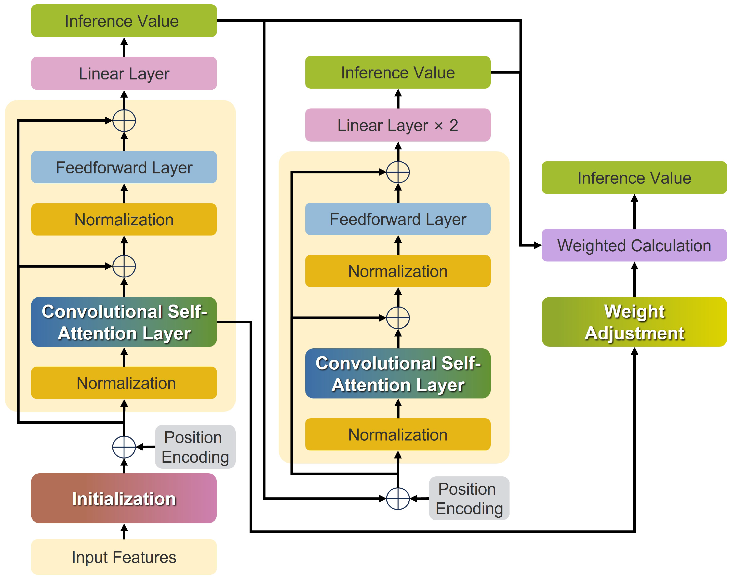
4.1. The Overall Architecture of the CTIM

The input of this CTIM is the fusion of feature matrices of multivariable time-series data, which contain a certain proportion of missing variables X, M, and $\mathrm{\Delta }$. The CTIM consists of three modules: an imputation module, reconstruction module, and weighted connection module, with the overall model framework depicted in Figure 2. The imputation module and reconstruction module are both composed of the fusion of features and convolutional improvements made to the attention mechanism. First, the imputed missing variables are filled in the original dataset, with the observed values remaining unchanged in the imputation module, and a new dataset ${\widehat{X}}_1$ is obtained. Second, the dataset ${\widehat{X}}_2$ is directly inputted into the reconstruction module to reconstruct the values of all positions (including the observed values), and the reconstruction sequence ${\widehat{X}}_3$ is obtained. The final complete sequence can be inferred by a set of learnable weights based on ${\widehat{X}}_1$ and ${\widehat{X}}_2$.

For the imputation module, the multivariable time-series data X and the mask matrix M are concatenated as an input matrix. The feature information is extracted by the improved self-attention, and then the missing values are deduced through a linear combination layer. The related formulas are shown as follows:

$$\left\{\begin{array}{c}{A}_1=\mathrm{SelfAttention}(X;M)\\ Z_1=FFN\left(A_1\right)\\ {\widehat{X}}_1^{\prime }=Z_1{W}_1+B_1\\ {\widehat{X}}_1=M\odot {\widehat{X}}_1^{\prime }+(1-M)\odot X\end{array}\right.$$

(8)

where ⨀ signifies the product of corresponding elements within the matrix, and FFN represents the feedforward layer. In the reconstruction module, ${\widehat{X}}_1$ is used as the input and two linear layers are used for inference:

$$\left\{\begin{array}{c}{A}_2=\mathrm{SelfAttention}({\widehat{X}}_1;M)\\ Z_2=FFN\left(A_2\right)\\ {\widehat{X}}_2=\mathrm{GELU}(Z_2{W}_a+B_a)W_b+B_b\end{array}\right.$$

(9)

where $A_i$ is the output of the self-attention layer and $Z_i$ is the output of the feedforward fully connected layer. The GELU activation function adopts the random regularization for calculation. The PRE-LN technology is used in the improved transformer model, which normalizes the values before the self-attention layer and the feedforward connection layer [40]. For a more accurate inference, the weight connection module is adopted to adjust the weights of ${\widehat{X}}_1$ and ${\widehat{X}}_2$:

$$\alpha =\mathrm{Softmax}\left(h_1/(h_1+h_2)\right)$$

(10)

where $h_1$ and $h_2$ are the linear transformations of the outputs of the self-attention layers. Adopting the threshold $\beta$ to adjust $\alpha$, the final weight can be represented as

$$\gamma =(1-M)\odot (\alpha +\beta )/2+M\odot \alpha$$

(11)

Then, the imputation values can be obtained and the completed multivariate time series can be formulated as follows:

$$\left\{\begin{array}{c}{\widehat{X}}_3^{\prime }=\gamma {\widehat{X}}_1+(1-\gamma ){\widehat{X}}_2\\ {\widehat{X}}_3=M\odot {\widehat{X}}_3^{\prime }+(1-M)\odot X\end{array}\right.$$

(12)

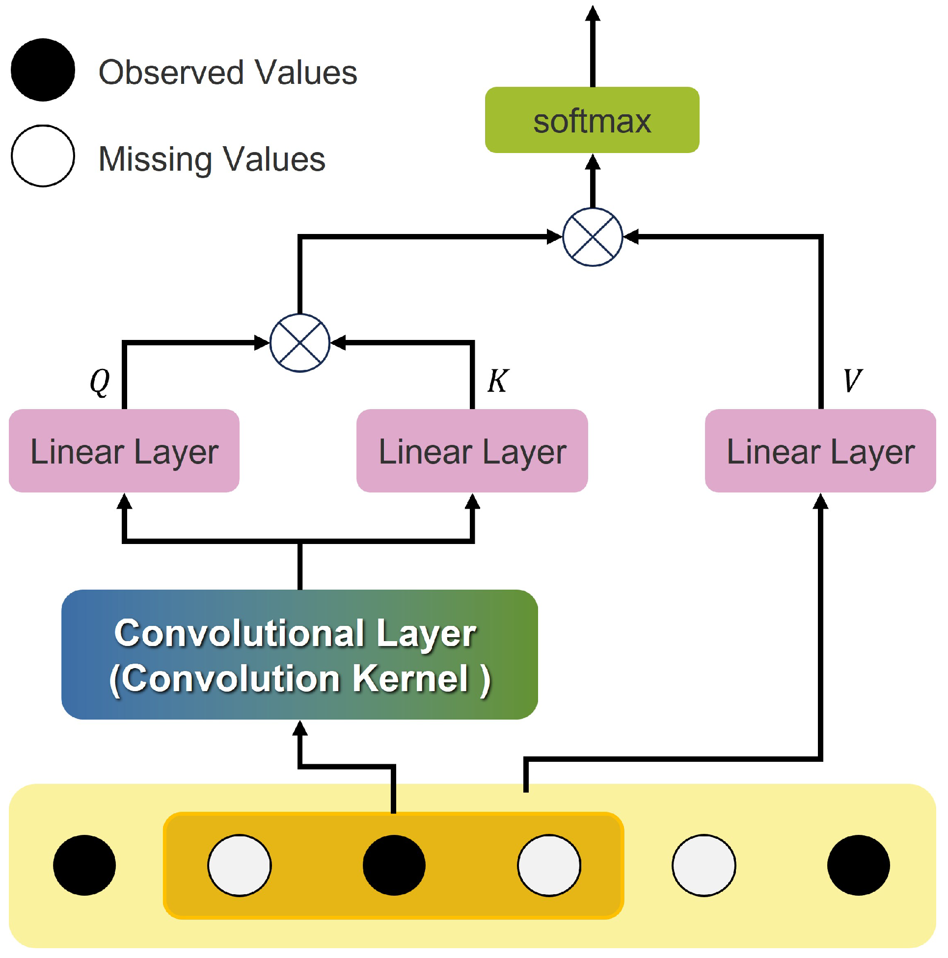
4.2. The Convolutional Self-Attention Layer

In the initial self-attention layer, the queries (Q), keys (K), and values (V) are obtained by a linear transformation (e.g., $Q=w_1{x}_1,w_2{x}_2,\cdots ,w_t{x}_t$). If $x_1$ and $x_2$ are similar vectors, the weights at these two moments will be confused when calculating the attention scores. For an incomplete dataset, when the missing proportion is too high, the extracted features will be highly similar due to the missing values being regarded as zeros, which will result in ineffective weights. In this study, a convolutional layer was adopted to capture the information around each component, the relationship between the time series, and different variables. Then, the output of the convolutional layer is used to calculate the correlations between the data Q, K, and values of the historical data V, which is shown in Figure 3.

The specific calculation process is as follows:

$$c=w_c(x_i,x_{i+1},\cdots ,x_{i+k})$$

(13)

where c is the information of the vector at time t and its neighboring vectors obtained from the convolutional layer $c=\left\{c_1,c_2,\cdots ,c_t\right\}$. The queries Q, keys K, and values V can be calculated as follows:

$$\left\{\begin{array}{c}{q}_t=c_t{w}_q+b_q\\ k_t=c_t{w}_k+b_k\\ v_t=x_t{w}_v+b_v\end{array}\right.$$

(14)

where $Q=\left\{q_1,q_2,\cdots ,q_t\right\}$, $K=\left\{k_1,k_2,\cdots ,k_t\right\}$, $V=\left\{v_1,v_2,\cdots ,v_t\right\}$, and w and b are the weight parameters. The output of the convolutional self-attention layer can be calculated as follows:

$$O=\mathrm{Softmax}(Q{K}^T/\sqrt{d_k})V$$

(15)

where $O\in R^{T\times E}$, E is the dimension number of the missing data, and $d_k$ is the number of columns in the matrix K.

4.3. Position Encoding

In the original transformer model, the self-attention layer cannot capture sequence information since there is no temporal loop mechanism. The order contains very important information in the sequential dataset, which means the position of each element should be considered in a time series. This article proposes a position encoding to add positional information to the sequence data. In the position encoding, the sine and cosine functions are used to generate time-varying waveforms, which are then superimposed on the input [41]. Sine and cosine have different values at different positions and can be used to represent the relative positions of two elements in a sequence:

$$\left\{\begin{array}{c}P{E}_{(pos,t)}=sin\left({\displaystyle \frac{t}{10,{000}^{2\frac{t}{E}}}}\right)\\ P{E}_{(pos,t+1)}=cos\left({\displaystyle \frac{t}{10,{000}^{2\frac{t+1}{E}}}}\right)\end{array}\right.$$

(16)

where t and $t+1$ mean the odd position encoding and even position encoding, respectively; E is the dimension number of the missing data.

4.4. The Loss Function

The choice of loss function significantly impacts the model performance and training stability. In this study, the mean absolute error (MAE) was used to represent the loss between the actual and produced values [42], which could provide constant gradients, and thus, prevent exploding gradient issues during training. The related calculation formulas are illustrated as follows:

$${\mathcal{L}}_{MAE}\left(x_t^d,{\widehat{x}}_t^d,m_t^d\right)={\displaystyle \frac{{\sum }_{d=1}^D{\sum }_{t=1}^T{m}_t^d\odot \left(x_t^d-{\widehat{x}}_t^d\right)}{{\sum }_{d=1}^D{\sum }_{t=1}^T{m}_t^d}}$$

(17)

(1) The synthesis loss: the synthesis loss, which measures the similarity between the predicted values ${\widehat{X}}_1$ and the ground-truth values X, is defined as

$${\mathcal{L}}_1={\mathcal{L}}_{MAE}(X,{\widehat{X}}_1,M)$$

(18)

(2) The reconstruction loss: the reconstruction loss is defined as the distance between the input and reconstructed values:

$${\mathcal{L}}_2={\mathcal{L}}_{MAE}(X,{\widehat{X}}_2,M)$$

(19)

(3) The adjustment loss: the adjustment loss can be expressed as

$${\mathcal{L}}_3={\mathcal{L}}_{MAE}(X,{\widehat{X}}_3,M)$$

(20)

where ${\mathcal{L}}_{MAE}$, ${\mathcal{L}}_1$, ${\mathcal{L}}_2$, and ${\mathcal{L}}_3$ are the formulas of the MAE and the errors of the imputation module, reconstruction module, and weighted connection module, respectively. Therefore, the overall loss is represented as

$${\mathcal{L}}_{total}={\lambda }_1{\mathcal{L}}_1+{\lambda }_2{\mathcal{L}}_2+{\lambda }_3{\mathcal{L}}_3$$

(21)

where ${\lambda }_1$, ${\lambda }_2$, and ${\lambda }_3$ are the weights for each loss term.

4.5. Training and Testing Process

The training and testing processes for handling missing multivariate time-series data followed a systematic approach. In the training phase, the original dataset was divided into training (80%) and testing (20%) sets. We generated mask matrices to simulate both continuous and random missing patterns, where the missing rates varied from 2% to 40%. The model training took the original data, mask matrix, and time intervals as inputs, which were optimized through the weighted loss function. Through this training process, the model learned to extract temporal dependencies using convolutional self-attention, capture variable correlations across different dimensions, and generate missing values while maintaining the original data distribution.

During the testing phase, the trained model first employed the imputation module to generate initial estimates for the missing values. These estimates were then refined through the reconstruction module, and the final predictions were obtained by combining results through the weighted connection mechanism. The model performance was evaluated using the MAE, RMSE, and MRE metrics, with 95% confidence intervals calculated through Monte Carlo simulations. To ensure result reliability, we implemented a K-fold cross-validation and conducted statistical significance tests across different missing rates and patterns.

5. Experimental Implementation

To assess the effectiveness of the proposed CTIM method, several algorithms were utilized in this experiment. The EM algorithm, whose main idea is to find the parameter $\theta$ to maximize the log-likelihood estimate $F=logf\left(x\right|\theta )$ for the incomplete data problem; the ARMA model, which combines the autoregressive process and the moving average process; the autoencoder, which generates missing data using the features obtained from the existing data; the generative adversarial network, which generates new samples by utilizing random noise, and the discriminator takes both the generated and original vectors as input and outputs the probability of each sample being real; and the LSTM model, which provides a short-term memory that can last thousands of time steps and is applicable to predicting data based on a time series. In this experiment, all the algorithms were implemented using the Python compiler framework and run on an NVIDIA GeForce GT610 and Intel (R) Xeon (R) CPUE5-2620v4@2.10 GHz environment.

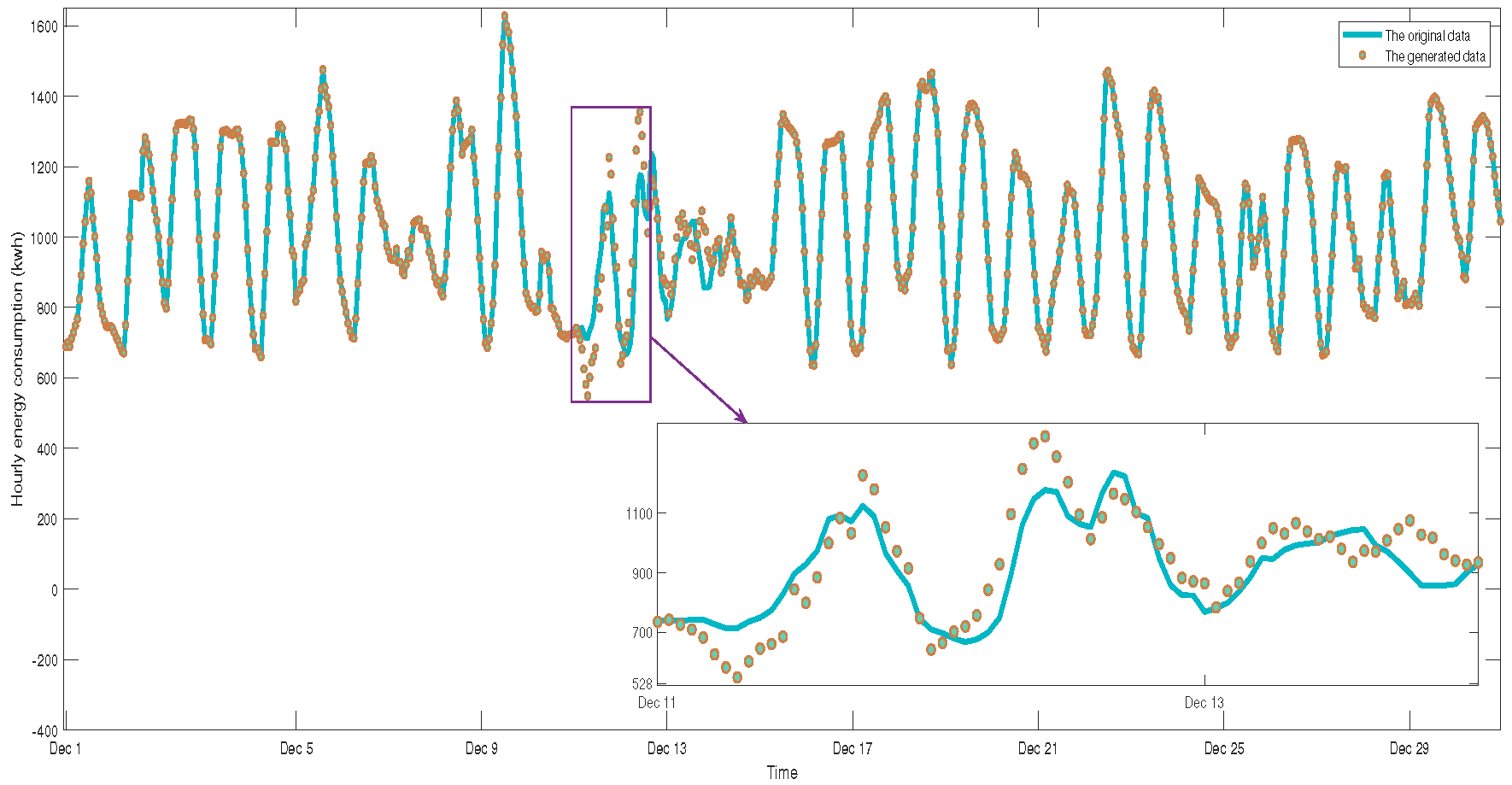
5.1. Industrial Data Set

In the industrial park, the electricity generated from renewable energy, electricity imported and exported to the power grid, and the heat generation from gas are the main resources for different plant rooms. This study provided an in-depth analysis of the initial dataset that captured energy generation and consumption within an industrial park over a randomly chosen time frame. Energy-related features were recorded at one-hour intervals: electricity power generated from a wind turbine and two CHP units, the heat supplied by four gas boilers, the heat load of six plant rooms, and the onsite electricity load of the whole industrial park. Each dimension in the dataset represents distinct signals that vary in scale; consequently, normalization was necessary to adjust all inputs to a comparable range [43]. In this experiment, we collected data from the industrial park that spanned a 30-day period that commenced on 1 December 2019. As illustrated in

Table 1. The electricity and heat datasets in the experiment.

Dataset	Attribution	Time	Initial Length
Electricity	10	31 days	744
Heat	14	31 days	744

, the normalized dataset comprised 744 samples, where each sample encompassed 24 distinct dimensions. This comprehensive dataset enabled detailed analysis and insights into energy patterns and behaviors over the specified time frame.

To simulate real-world scenarios of missing data, we randomly selected varying percentages of the original dataset and designated them as NaN, which represented the missing data. In our experiment, the missing data percentages were set at 2, 5, 10, 15, 20, 25, 30, 35, and 40 percent, resulting in data matrices denoted as $D_2$, $D_5$, $D_{10}$, $D_{15}$, $D_{20}$, $D_{25}$, $D_{30}$, $D_{35}$, and $D_{40}$. In order to reflect the reality of data collection in industrial applications, there were two types of missing data: missing for a period (i.e., continuous missing data) and missing completely at random (i.e., random missing data). We defined the state of missing for a period as state 1, and the state of missing completely at random as state 2. In state 1, data were missing continuously over a random time span, which created gaps that mimic real-world scenarios where data may be lost due to a sensor failure or communication issues. In state 2, the dataset contained samples with missing values randomly distributed throughout, which simulated scenarios where data points were lost sporadically due to random errors or noise.

5.2. Experimental Setup

The parameters of algorithms in the experiment were set as follows. The EM algorithm adopted a Gaussian probability function and maximum likelihood estimation. For the ARIMA model, the optimal parameters p and q were determined based on ACF and PACF diagrams, respectively [44]. For the autoencoder, the number of latent representations was set to be K. As for a GAN, both the generator and discriminator shared identical architectures, where each comprised three layers. The generator’s layers consisted of 100, 512, and K nodes, while the discriminator’s layers were structured with K, 512, and 1 nodes, respectively. The hidden layers utilized the sigmoid activation function, and the output layers employed the ReLU activation function. For mini-batch gradient descent, each mini-batch contained 100 samples. The model was trained over 400 iterations with a learning rate set at 0.001. For the autoencoder and GAN, the number of latent features K were set to be $floor(n/5)$, where n represents the total number of attributes in the original dataset. For the LSTM, the number of epochs was set to be 400 and the dropout rate was 15%.

In the experiment, a total of 744 samples were randomly selected from the original dataset to serve as the real data. To evaluate the accuracy of the missing value imputation, the expert assessment used the total root-mean-squared error (RMSE), the mean absolute error (MAE), the mean relative error (MRE), and the structural similarity index (SSIM) as the evaluation criteria [45]. The RMSE effectively measures the deviations in distances between the actual and generated points. The MAE indicates the average absolute error between the predicted and actual values. The MRE can reflect the reliability of measurements. The formulas of the four indicators are as follows:

$$\mathrm{RMSE}(X,\widehat{X})={\displaystyle \frac{{\sum }_{d=1}^D{\sum }_{t=1}^T({(x_t^d-\widehat{x_t^d})}^2\times m_t^d)}{{\sum }_{d=1}^D{\sum }_{t=1}^T{m}_t^d}}$$

(22)

$$\mathrm{MAE}(X,\widehat{X})={\displaystyle \frac{{\sum }_{d=1}^D{\sum }_{t=1}^T|(x_t^d-\widehat{x_t^d})\times m_t^d|}{{\sum }_{d=1}^D{\sum }_{t=1}^T{m}_t^d}}$$

(23)

$$\mathrm{MRE}(X,\widehat{X})={\displaystyle \frac{{\sum }_{d=1}^D{\sum }_{t=1}^T((x_t^d-\widehat{x_t^d})\times m_t^d)}{{\sum }_{d=1}^D{\sum }_{t=1}^T{m}_t^d\times x_t^d}}$$

(24)

$$\mathrm{SSIM}(X,\widehat{X})=\left[l(x,\widehat{X})\right]·\left[c(x,\widehat{X})\right]·\left[s(x,\widehat{X})\right]$$

(25)

where R is the number of dimensions in the output, $x_i$ represents the i-th dimension of the actual data, and $\widehat{x_i}$ denotes the i-th dimension of the generated data. $l(x,\widehat{X})$, $c(x,\widehat{X})$, and $s(x,\widehat{X})$ measure the luminance, contrast, and structural similarity, respectively:

$$l(x,\widehat{X})=(2\mu x\mu \widehat{x}+C_1)/(\mu x^2+\mu {\widehat{x}}^2+C_1)$$

(26)

$$c(x,\widehat{X})=(2\sigma x\sigma \widehat{x}+C_2)/(\sigma x^2+\sigma {\widehat{x}}^2+C_2)$$

(27)

$$s(x,\widehat{X})=(2\sigma x\widehat{x}+C_3)/(\sigma x\sigma \widehat{x}+C_3)$$

(28)

where $\mu x$ and $\mu \widehat{x}$ are the mean values of sequences x and $\widehat{x}$; $\sigma x$ and $\sigma \widehat{x}$ are the standard deviations; $\sigma x\widehat{x}$ is the covariance between x and $\widehat{x}$; and $C_1$, $C_2$, and $C_3$ are small constants to avoid division by zero.

5.3. Hyperparameter Configuration

In this study, we configured the hyperparameters to achieve the optimal performance of the proposed model. For the learning process, the initial learning rate was 0.01, and training was conducted with a batch size of 64 over 100 epochs. For the transformer architecture, the final configuration consisted of four transformer layers, where each contained four attention heads. The embedding dimension was set to 128, with a feedforward dimension of 512. A dropout rate of 0.1 was applied throughout the network to enhance the regularization. The loss weights in Equation (21) were initialized as ${\lambda }_1=0.33,{\lambda }_2=0.33$, and ${\lambda }_3=0.33$, which balanced the importance between the imputation, reconstruction, and weighted connection modules.

6. Experiment Results and Discussion

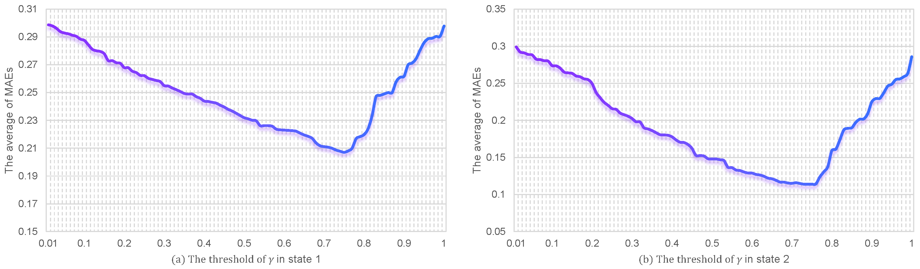
6.1. The Weight Threshold

Two transformer modules were adopted in the proposed algorithm. Based on the information learned by the self-attention layer in the two modules, the inference values were weighted by $\gamma$ to obtain the final result. Thus, the preset weight threshold could be adjusted to reduce or increase the weight $\gamma$. In order to verify the impact of different weight threshold on the proposed algorithm, this study set the threshold to 0–1 and the step size to 0.01, and verified the performance changes of the model on two states with 15% missing rates under different weight thresholds.

Monte Carlo simulation is a computational technique that models a random process to solve problems, helping to understand the impact of risk and uncertainty due to inherent randomness [46]. In this experiment, we repeated the procedure 200 times using the Monte Carlo method. The result that was closest to the average value of the outputs was selected as the final outcome. Figure 4 presents the mean values of the MAEs under different weight thresholds for both states. The two subplots, (a) and (b), illustrate the MAEs for 200 samples in state 1 and state 2, respectively. According to the Monte Carlo method, the results for both continuous and random missing data states were obtained from the 97th and 135th simulations. It was obvious that when the threshold of weight $\gamma$ was set to 0.75, the proposed imputation model performed the best. The changes in the model performance under different thresholds reflect that setting weight thresholds could adjust the accuracy of the model imputation.

Additionally, we employed the generated data samples from the proposed model using a weight threshold of 0.75 to fill in the gaps for both the continuous and random missing data scenarios. We then calculated the energy consumption based on the generated data and compared it with the actual energy usage over the selected one-month period. Figure 5 and Figure 6 illustrate the hourly energy consumption during the missing data period, showing comparisons between the generated data and the real data for state 1 (continuous missing) and state 2 (random missing), respectively. Although there was a minor variation between the real and generated data concerning the hourly energy consumption for the combined heat and power system in the industrial park, the average difference was below 10%, which was considered satisfactory by the technicians at the industrial plants.

6.2. Computational Complexity

The computational complexity of our model mainly comes from two components: the convolutional operations and the self-attention mechanism. For a time series with length T and dimension D, the traditional self-attention (SA) has a quadratic complexity of $O\left(T^{2}D\right)$. Our convolutional self-attention reduces this to $O(K{T}^{2}D/r^2)$, where K is the kernel size and r is the reduction ratio from our local attention design. By incorporating local attention windows ($r<<T$) and convolutional operations with the kernel size, we achieved significant computational savings while maintaining the model performance. To quantify the efficiency gains, we conducted runtime comparisons and show the results in

Table 2. Computational efficiency comparison.

Model	Training Time (s/epoch)	Memory Usage (GB)
Traditional SA	145	3.2
The proposed model	82	1.8
Reduction	43.4%	43.8%

. These results demonstrate that the proposed approach achieved better computational efficiency while maintaining a competitive imputation accuracy.

6.3. Continuous Missing vs. Random Missing

The continuous missing and random missing states are the two typical scenarios in reality. To explore the difference between these two situations, the average root-mean-squared error $\overline{R}$, In(Mean), sensitivity to missing rates, and 95% confidence interval (CI) are introduced in this article. First, In(Mean) denotes the enhancement in average RMSE across different imputations, expressed as follows:

$$\mathrm{In}\left(\mathrm{Mean}\right)={\displaystyle \frac{\overline{R}-{\overline{R}}_{Mean}}{{\overline{R}}_{Mean}}}$$

(29)

where $\overline{R}$ represents the average root-mean-squared error of the method under different missing rates. Second, the sensitivity to missing rates is used to measure the effect of various missing rates. The sensitivity can be computed using the slope value between $mr$ and $\overline{R}$, as indicated below:

$$S_m={\displaystyle \frac{{\sum }_{i=1}^n(m{r}_i-\overline{mr})(R_i-\overline{R})}{{\sum }_{i=1}^n{(m{r}_i-\overline{mr})}^2}}$$

(30)

where $mr$ means the missing rates. The comparison of the continuous missing and random missing states with the classical methods and the proposed algorithm is shown in

Table 3. Performance comparison between continuous and random missing states.

Methods	State 1 (Continuous Missing)				State 2 (Random Missing)
	$\overline{\mathit{R}}$	In(Mean)	Sensitivity	95% CI of MAE	$\overline{\mathit{R}}$	In(Mean)	Sensitivity	95% CI of MAE
EM	0.2382	0.05%	0.0032	0.278 ± 0.022	0.1643	0.01%	0.0013	0.191 ± 0.015
ARIMA	0.2061	2.19%	0.0100	0.241 ± 0.019	0.1402	40.59%	0.0370	0.163 ± 0.013
Autoencoder	0.1790	13.38%	0.0162	0.209 ± 0.016	0.1177	34.99%	0.0275	0.137 ± 0.011
GAN	0.1581	20.09%	0.0150	0.185 ± 0.014	0.1018	29.67%	0.0245	0.119 ± 0.010
LSTM	0.1610	18.42%	0.0149	0.188 ± 0.014	0.1014	31.82%	0.0244	0.118 ± 0.009
The proposed model	0.1351	11.10%	0.0096	0.158 ± 0.012	0.0875	14.85%	0.0218	0.102 ± 0.008

. It is evident that the average root-mean-squared error $\overline{R}$ for the continuous missing state was significantly higher than for the random missing state. This observation was further supported by the 95% CI of the MAE, where the continuous missing state showed consistently wider confidence intervals (e.g., EM: 0.278 ± 0.022 vs. 0.191 ± 0.015) compared with the random missing state, indicating greater uncertainty in the predictions for the continuous missing data. This indicates that continuous missing values are more challenging to predict than random missing values at the same missing rate. This is expected, as there is less information available from neighboring data points in the continuous missing state. Consequently, both the proposed algorithm and other conventional methods performed less effectively when addressing continuous missing data compared with random missing data.

For the random missing state, the EM algorithm could achieve an accuracy of 0.01% for the mean imputation. In contrast, for the continuous missing state, even the proposed algorithm only reached an In(Mean) value of 11.1%. This observation was further supported by the 95% CI of the MAE, where the continuous missing state showed consistently wider confidence intervals compared with the random missing state, indicating a greater uncertainty in predictions for continuous missing data. This suggests that mean imputation was preferable for handling continuous missing data over model-based methods, considering the computational effort required for training and testing. As for the sensitivity value, the proposed model was slightly worse than EM and better than the other classical methods.

The proposed algorithm achieved an outstanding performance in both the random missing and continuous missing data situations, which obtained benefits from the convolutional self-attention module and weighted techniques. The stability of our model was evidenced by its consistently smaller confidence intervals across both states compared with the classical methods. The convolutional self-attention layer could help the model obtain more information nearby, and the weighted module adjusted the prediction of the two transformer modules. In conclusion, the proposed algorithm had more robustness in both the random missing state and the continuous missing state, as demonstrated by both the performance metrics and confidence intervals.

6.4. Effects of Different Missing Data Ratios

The more data we have, the richer information we can obtain from the sequence, which means a more accurate potential distribution of the data can be captured. To assess the imputation performances of the proposed model across various missing data rates, we randomly removed 2%, 5%, 10%, 15%, 20%, 25%, 30%, 35%, and 40% of the observed data. The boxing plots based on the distribution of MAE values for the continuous missing and random missing states in 200 Monte Carlo experiments are shown in Figure 7, displaying the maximum and minimum values, median, quartiles, and third quartiles. It is obvious that not only the average value of the MAEs but also the overall distribution of MAE values showed a trend of increasing with the increase in the data missing rate, which is consistent with the results analysis in the previous text. In addition, as the missing rate of data increased, the distribution range and extreme range of the fourth to third quartiles of the MAE also expanded, indicating that the stability of the model imputation also decreased with the loss of latent features. It was difficult to impute the missing data with limited information, which resulted in significant errors.

The MAE, RMSE, MRE, and SSIM values were used to compare the performances of the proposed CTIM and the other classical methods, as shown in Figure 8, Figure 9, Figure 10 and Figure 11 respectively. It is obvious that the trends of the evaluation indexes increased with the missing ratios in the two states. When the missing data ratio was low, specifically at 2% and 5%, the classical methods performed comparably with the proposed model. Meanwhile, the difference between the various methods and the proposed model became wider as the missing ratio became bigger. Among these methods, the proposed CTIM achieved the best performance, while the EM performed the worst. This was expected for the EM method due to the classical and simple calculation, which cannot learn anything from the training dataset. And thus, the EM method performed poorly in the missing data generation and was sensitive to the outliers, which means the advanced algorithms were far superior to the classical method. The ARIMA model was more effective than EM, but still worse than the generative methods, such as the autoencoder and GAN. The performance of LSTM was almost the same as that of the GAN for the MAE indicator, which means the effects of the two strategies were almost similar.

In the state of continuous missing, the RMSE values of the proposed CTIM were 6.78%, 7.62%, 7.66%, 7.84%, 5.68%, 6.13%, 9.51%, 9.49%, and 4.92% lower than those of LSTM across the range of missing ratios from 2% to 40%, respectively. As for the state of random missing, the proposed CTIM produced similar results, where the RMSE values were 14.49%, 17.24%, 10.74%, 13.77%, 9.98%, 17.66%, 17.77%, 16.07%, and 9.23% lower than those of the following algorithm, respectively. State 2 achieved higher SSIM scores than state 1, with the performance gap widening as missing ratios increased. For low missing ratios (2–10%), the CTIM maintained high performance with SSIM > 0.93 in state 1 and >0.95 in state 2, while the traditional methods showed acceptable performance (SSIM > 0.88). At medium missing ratios (15–25%), the deep learning methods maintained robust performances in both states (state 1 > 0.86, state 2 > 0.88), where the CTIM showed a consistent 2–3% advantage over the other methods. Under high missing ratios (30–40%), state 1 exhibited significant performance degradation (SSIM < 0.85), while state 2 better preserved the data structure (SSIM > 0.87).

Furthermore, the experimental results reveal that the convolutional transformer imputation model this article proposes based on the robust technique prevailed over the other comparative methods. The obvious reason for these phenomena was the combination of the convolution layer and self-attention layer, which had high asymptotic efficiency of the features of existing data. For the error criteria, the proposed CTIM technique produced lower errors than the other methods. The experimental simulations demonstrated clearly that the CTIM technique was the most effective missing data imputation method for reconstructing missing energy data.

In conclusion, several conclusions can be drawn as follows: First, the MAE, RMSE, MRE, and SSIM all increased with the increase in the missing rate, meaning that the performance of each model decreased. The imputation performance of various models was directly affected by the missing rate. Second, the core of the proposed algorithm in this article is the convolutional layer and self-attention mechanism in the transformer, which led to the filling performance at different missing rates achieving good filling effects, indicating high inference reliability of the model. These results demonstrate the effectiveness of the convolutional transformer imputation model. Third, the imputation method proposed in this article achieved a good performance through three evaluation criteria under different missing rates, reflecting the value of the imputation model in filling incomplete multivariate time-series missing data applications.

When the missing data rate was below 40%, the model demonstrated robust performance by maintaining reliable temporal pattern reconstruction. This indicates that the proposed model could effectively learn and capture the underlying data patterns for accurate imputation with sufficient information. However, when the missing data proportion exceeded 40%, there was a substantial degradation in the model performance. The MAE, RMSE, and MRE values increased significantly, and the model’s ability to reconstruct temporal patterns became unreliable. This performance could have been caused by the insufficient information available for the model to learn meaningful patterns. With high missing rates, the remaining data could not provide adequate information to capture the complex relationships in the industrial time-series data.

6.5. Bias Analysis and Mitigation Strategies

Missing data imputation in real-world industrial applications requires the careful consideration of potential biases and corresponding mitigation strategies. The convolutional transformer architecture may introduce model architecture bias through attention mechanism preferences, convolution kernel size limitations, and feature representation imbalances. The time-series nature of data presents another source of potential bias through temporal dependencies, seasonal patterns, and transitions between different operating modes.

To address these identified biases, we implemented a set of mitigation strategies. The enhanced model architecture incorporates several technical improvements to minimize potential biases. We applied dropout layers with a 10% rate to prevent overfitting, implementing weighted loss functions to balance the influence of different data patterns, and utilized ensemble predictions from multiple model initializations to improve the robustness. In addition, we conducted cross-validation across different temporal segments to ensure consistent performance across various time periods. The model adopted a performance evaluation under diverse operational conditions (with the missing rates being 2–40%) to verify its reliability. This validation approach helped ensure that our model maintains high accuracy and reliability in real-world industrial applications.

6.6. Robustness Analysis of CTIM Model

To evaluate the resilience of the proposed model under challenging real-world scenarios, we conducted experiments with adversarially perturbed missing patterns.

(1) For the noise-induced missing situation, we introduced Gaussian noise (with the standard deviation $\sigma$ being 0.1, 0.2, and 0.3) to the mask matrix M to simulate sensor measurement errors that affected the missing data patterns. The proposed CTIM maintained a stable performance with only 5–7% degradation in the MAE values when $\sigma \le 0.2$, thus demonstrating robust feature extraction capabilities. (2) For the anomaly-influenced missing scenario, we simulated sudden equipment failures by introducing burst missing periods (30–60 consecutive timestamps) at random locations. The proposed model showed a small amount of degradation but maintained an RMSE under 0.15 when there were less than three burst periods within the test window, which benefited from the convolutional self-attention mechanism to leverage both local and global temporal dependencies.

The experimental results demonstrate that the proposed CTIM exhibited strong robustness against both gradual noise perturbations and sudden anomalous missing patterns. This resilience can be attributed to the following: (1) the convolutional layer could extract stable local features even under noisy conditions; (2) the self-attention mechanism could identify and leverage long-range dependencies when local patterns were disrupted. These findings suggest that the CTIM is well-suited for real industrial deployments where sensor noise and equipment anomalies are common.

6.7. Online Adaptation and Model Extension

The proposed CTIM would demonstrate adaptability to online/streaming scenarios through several key modifications: (1) A sliding window mechanism enables incremental processing of incoming data streams and the model parameter updates based on the most recent window. (2) For real-time processing, the system maintains a buffer for incoming data points, triggers online learning at a threshold, and dynamically updates the transformer attention weights. (3) Computational efficiency is achieved through progressive attention matrix updates and optimized memory usage via selective feature retention.

In addition, the proposed CTIM can be augmented with statistical methods for improving the robustness and validation. For instance, the proposed model can incorporate Kalman filtering for sequential state estimation. The CTIM could also employ statistical tests for outlier detection and data quality assessment.

7. Conclusions

This paper presents the energy-monitoring system created by Point Energy Technology, which is intended to track and document the operational status of industrial machinery. During the data collection process, it was observed that data were often missing for various reasons. To address the missing data, we propose a convolutional transformer imputation model based on self-attention for data augmentation. This model comprises three modules: the imputation module, the reconstruction module, and the weighted connection module, all working together to reconstruct missing data. To extract the distribution features of industrial data, the model utilizes historical and future sequence information through an enhanced masking mechanism, along with convolution and self-attention for capturing local dependency information.

For evaluating the effectiveness of the proposed imputation model, we used a multivariable time-series dataset from a local industrial park collected over a randomly selected one-month period in 2019. We explored two types of missing data: continuous missing and random missing. The experimental results can be summarized as follows: (i) The MAE, RMSE, MRE, and SSIM values increased with the missing rate, indicating a decline in the model performance. (ii) The combination of convolution and self-attention effectively extracted the distribution features from the multivariable time-series data, as evidenced by the superior performance of the proposed model. (iii) The proposed data augmentation technique allowed for sufficiently reliable data analysis, which enabled us to make informed professional recommendations for our industrial partners. (iv) The potential biases and mitigation strategies are also discussed in this article.

References

1. Schafer, J.L.; Olsen, M.K. Multiple imputation for multivariate missing-data problems: A data analyst’s perspective. Multivar. Behav. Res. 1998, 33, 545–571. [Google Scholar] [CrossRef] [PubMed]
2. Reinsel, G.C. Elements of Multivariate Time Series Analysis; Springer Science & Business Media: Berlin/Heidelberg, Germany, 2003. [Google Scholar]
3. Li, J.; Izakian, H.; Pedrycz, W.; Jamal, I. Clustering-based anomaly detection in multivariate time series data. Appl. Soft Comput. 2021, 100, 106919. [Google Scholar] [CrossRef]
4. Li, L.; Zhang, J.; Wang, Y.; Ran, B. Missing value imputation for traffic-related time series data based on a multi-view learning method. IEEE Trans. Intell. Transp. Syst. 2018, 20, 2933–2943. [Google Scholar] [CrossRef]
5. Wu, R.; Hamshaw, S.D.; Yang, L.; Kincaid, D.W.; Etheridge, R.; Ghasemkhani, A. Data imputation for multivariate time series sensor data with large gaps of missing data. IEEE Sensors J. 2022, 22, 10671–10683. [Google Scholar] [CrossRef]
6. Park, J.; Müller, J.; Arora, B.; Faybishenko, B.; Pastorello, G.; Varadharajan, C.; Sahu, R.; Agarwal, D. Long-term missing value imputation for time series data using deep neural networks. Neural Comput. Appl. 2023, 35, 9071–9091. [Google Scholar] [CrossRef]
7. Wang, T.; Ke, H.; Jolfaei, A.; Wen, S.; Haghighi, M.S.; Huang, S. Missing value filling based on the collaboration of cloud and edge in artificial intelligence of things. IEEE Trans. Ind. Inform. 2021, 18, 5394–5402. [Google Scholar] [CrossRef]
8. Luo, Y.; Cai, X.; Zhang, Y.; Xu, J. Multivariate time series imputation with generative adversarial networks. Adv. Neural Inf. Process. Syst. 2018, 31. [Google Scholar]
9. Zhao, J.; Rong, C.; Lin, C.; Dang, X. Multivariate time series data imputation using attention-based mechanism. Neurocomputing 2023, 542, 126238. [Google Scholar] [CrossRef]
10. Cismondi, F.; Fialho, A.S.; Vieira, S.M.; Reti, S.R.; Sousa, J.M.; Finkelstein, S.N. Missing data in medical databases: Impute, delete or classify? Artif. Intell. Med. 2013, 58, 63–72. [Google Scholar] [CrossRef]
11. King, G.; Honaker, J.; Joseph, A.; Scheve, K. List-wise deletion is evil: What to do about missing data in political science. In Proceedings of the Annual Meeting of the American Political Science Association, Boston, MA, USA, 3–6 September 1998; Volume 52. [Google Scholar]
12. Zhang, H.; Yue, D.; Dou, C.; Xie, X.; Li, K.; Hancke, G.P. Resilient optimal defensive strategy of TSK fuzzy-model-based microgrids’ system via a novel reinforcement learning approach. IEEE Trans. Neural Netw. Learn. Syst. 2021, 34, 1921–1931. [Google Scholar] [CrossRef]
13. Abu Alfeilat, H.A.; Hassanat, A.B.; Lasassmeh, O.; Tarawneh, A.S.; Alhasanat, M.B.; Eyal Salman, H.S.; Prasath, V.S. Effects of distance measure choice on k-nearest neighbor classifier performance: A review. Big Data 2019, 7, 221–248. [Google Scholar] [CrossRef] [PubMed]
14. Cheng, D.; Zhang, S.; Deng, Z.; Zhu, Y.; Zong, M. k NN algorithm with data-driven k value. In Proceedings of the Advanced Data Mining and Applications: 10th International Conference, ADMA 2014, Guilin, China, 19–21 December 2014; Proceedings 10. Springer: Berlin/Heidelberg, Germany, 2014; pp. 499–512. [Google Scholar]
15. Zhang, S.; Li, X.; Zong, M.; Zhu, X.; Cheng, D. Learning k for knn classification. ACM Trans. Intell. Syst. Technol. (TIST) 2017, 8, 43. [Google Scholar] [CrossRef]
16. Moon, T.K. The expectation-maximization algorithm. IEEE Signal Process. Mag. 1996, 13, 47–60. [Google Scholar] [CrossRef]
17. Fessler, J.A.; Hero, A.O. Space-alternating generalized expectation-maximization algorithm. IEEE Trans. Signal Process. 1994, 42, 2664–2677. [Google Scholar] [CrossRef]
18. Zhang, K.; Gonzalez, R.; Huang, B.; Ji, G. Expectation–maximization approach to fault diagnosis with missing data. IEEE Trans. Ind. Electron. 2014, 62, 1231–1240. [Google Scholar] [CrossRef]
19. Chen, L.; Wu, Z.; Cao, J.; Zhu, G.; Ge, Y. Travel recommendation via fusing multi-auxiliary information into matrix factorization. ACM Trans. Intell. Syst. Technol. (TIST) 2020, 11, 1–24. [Google Scholar] [CrossRef]
20. He, X.; Tang, J.; Du, X.; Hong, R.; Ren, T.; Chua, T.S. Fast matrix factorization with nonuniform weights on missing data. IEEE Trans. Neural Netw. Learn. Syst. 2019, 31, 2791–2804. [Google Scholar] [CrossRef]
21. Wu, P.; Pei, M.; Wang, T.; Liu, Y.; Liu, Z.; Zhong, L. A Low-Rank Bayesian Temporal Matrix Factorization for the Transfer Time Prediction Between Metro and Bus Systems. IEEE Trans. Intell. Transp. Syst. 2024, 25, 7206–7222. [Google Scholar] [CrossRef]
22. Žitnik, M.; Zupan, B. Data fusion by matrix factorization. IEEE Trans. Pattern Anal. Mach. Intell. 2014, 37, 41–53. [Google Scholar] [CrossRef]
23. Zhang, H.; Yue, D.; Yue, W.; Li, K.; Yin, M. MOEA/D-based probabilistic PBI approach for risk-based optimal operation of hybrid energy system with intermittent power uncertainty. IEEE Trans. Syst. Man, Cybern. Syst. 2019, 51, 2080–2090. [Google Scholar] [CrossRef]
24. Batista, G.E.; Monard, M.C. An analysis of four missing data treatment methods for supervised learning. Appl. Artif. Intell. 2003, 17, 519–533. [Google Scholar] [CrossRef]
25. Gómez, V.; Maravall, A.; Peña, D. Missing observations in ARIMA models: Skipping approach versus additive outlier approach. J. Econom. 1999, 88, 341–363. [Google Scholar] [CrossRef]
26. Abiri, N.; Linse, B.; Edén, P.; Ohlsson, M. Establishing strong imputation performance of a denoising autoencoder in a wide range of missing data problems. Neurocomputing 2019, 365, 137–146. [Google Scholar] [CrossRef]
27. Kang, M.; Zhu, R.; Chen, D.; Liu, X.; Yu, W. CM-GAN: A cross-modal generative adversarial network for imputing completely missing data in digital industry. IEEE Trans. Neural Netw. Learn. Syst. 2023, 35, 2917–2926. [Google Scholar] [CrossRef]
28. Che, Z.; Purushotham, S.; Cho, K.; Sontag, D.; Liu, Y. Recurrent neural networks for multivariate time series with missing values. Sci. Rep. 2018, 8, 6085. [Google Scholar] [CrossRef] [PubMed]
29. Han, K.; Xiao, A.; Wu, E.; Guo, J.; Xu, C.; Wang, Y. Transformer in transformer. Adv. Neural Inf. Process. Syst. 2021, 34, 15908–15919. [Google Scholar]
30. Goodfellow, I.; Pouget-Abadie, J.; Mirza, M.; Xu, B.; Warde-Farley, D.; Ozair, S.; Courville, A.; Bengio, Y. Generative adversarial nets. In Proceedings of the Advances in Neural Information Processing Systems, Montreal, QC, Canada, 8–13 December 2014; pp. 2672–2680. [Google Scholar]
31. Bianchi, F.M.; Livi, L.; Mikalsen, K.Ø.; Kampffmeyer, M.; Jenssen, R. Learning representations of multivariate time series with missing data. Pattern Recognit. 2019, 96, 106973. [Google Scholar] [CrossRef]
32. Ma, J.; Cheng, J.C.; Jiang, F.; Chen, W.; Wang, M.; Zhai, C. A bi-directional missing data imputation scheme based on LSTM and transfer learning for building energy data. Energy Build. 2020, 216, 109941. [Google Scholar] [CrossRef]
33. Yu, Y.; Si, X.; Hu, C.; Zhang, J. A review of recurrent neural networks: LSTM cells and network architectures. Neural Comput. 2019, 31, 1235–1270. [Google Scholar] [CrossRef]
34. Tian, Y.; Zhang, K.; Li, J.; Lin, X.; Yang, B. LSTM-based traffic flow prediction with missing data. Neurocomputing 2018, 318, 297–305. [Google Scholar] [CrossRef]
35. Tang, B.; Matteson, D.S. Probabilistic transformer for time series analysis. Adv. Neural Inf. Process. Syst. 2021, 34, 23592–23608. [Google Scholar]
36. Zerveas, G.; Jayaraman, S.; Patel, D.; Bhamidipaty, A.; Eickhoff, C. A transformer-based framework for multivariate time series representation learning. In Proceedings of the 27th ACM SIGKDD Conference on Knowledge Discovery & Data Mining, Virtual, 14–18 August 2021; pp. 2114–2124. [Google Scholar]
37. Han, K.; Wang, Y.; Chen, H.; Chen, X.; Guo, J.; Liu, Z.; Tang, Y.; Xiao, A.; Xu, C.; Xu, Y.; et al. A survey on vision transformer. IEEE Trans. Pattern Anal. Mach. Intell. 2022, 45, 87–110. [Google Scholar] [CrossRef]
38. Liu, J.; Pasumarthi, S.; Duffy, B.; Gong, E.; Datta, K.; Zaharchuk, G. One model to synthesize them all: Multi-contrast multi-scale transformer for missing data imputation. IEEE Trans. Med. Imaging 2023, 42, 2577–2591. [Google Scholar] [CrossRef] [PubMed]
39. Kline, J.; Kline, C. Power modeling for an industrial installation. In Proceedings of the Cement Industry Technical Conference, 2017 IEEE-IAS/PCA, Calgary, AB, Canada, 21–25 May 2017; pp. 1–10. [Google Scholar]
40. Wang, H.; Ma, S.; Dong, L.; Huang, S.; Zhang, D.; Wei, F. Deepnet: Scaling transformers to 1000 layers. IEEE Trans. Pattern Anal. Mach. Intell. 2024, 46, 6761–6774. [Google Scholar] [CrossRef]
41. Kazemnejad, A.; Padhi, I.; Natesan Ramamurthy, K.; Das, P.; Reddy, S. The impact of positional encoding on length generalization in transformers. Adv. Neural Inf. Process. Syst. 2023, 36, 24892–24928. [Google Scholar]
42. Hodson, T.O. Root mean square error (RMSE) or mean absolute error (MAE): When to use them or not. Geosci. Model Dev. Discuss. 2022, 15, 5481–5487. [Google Scholar] [CrossRef]
43. Liu, Y.; Cao, J.; Li, B.; Lu, J. Normalization and solvability of dynamic-algebraic Boolean networks. IEEE Trans. Neural Netw. Learn. Syst. 2018, 29, 3301–3306. [Google Scholar] [CrossRef]
44. Zahari, F.Z.; Khalid, K.; Roslan, R.; Sufahani, S.; Mohamad, M.; Rusiman, M.S.; Ali, M. Forecasting natural rubber price in Malaysia using ARIMA. J. Physics: Conf. Ser. 2018, 995, 012013. [Google Scholar] [CrossRef]
45. Wahbah, M.; El-Fouly, T.H.; Zahawi, B.; Feng, S. Hybrid beta-KDE model for solar irradiance probability density estimation. IEEE Trans. Sustain. Energy 2019, 11, 1110–1113. [Google Scholar] [CrossRef]
46. Mesleh, R.; Ikki, S.S.; Aggoune, H.M. Quadrature spatial modulation. IEEE Trans. Veh. Technol. 2015, 64, 2738–2742. [Google Scholar] [CrossRef]
Figure 1. The energy-monitoring system.
Symmetry 17 00686 g001
Figure 2. The overall architecture of the proposed algorithm.
Symmetry 17 00686 g002
Figure 3. The convolutional self-attention layer.
Symmetry 17 00686 g003
Figure 4. The Monte Carlo results of the two states.
Symmetry 17 00686 g004
Figure 5. The real and generated data for the continuous missing state.
Symmetry 17 00686 g005
Figure 6. The real and generated data for the random missing state.
Symmetry 17 00686 g006
Figure 7. The MAE values in the two states.
Symmetry 17 00686 g007
Figure 8. The MAE values in the two states.
Symmetry 17 00686 g008
Figure 9. The RMSE values in the two states.
Symmetry 17 00686 g009
Figure 10. The MRE values in the two states.
Symmetry 17 00686 g010
Figure 11. The SSIM values in the two states.
Symmetry 17 00686 g011