Fractional and Higher Integer-Order Moments for Fractional Stochastic Differential Equations

Abstract

This study investigates the computation of fractional and higher integer-order moments for a stochastic process governed by a one-dimensional, non-homogeneous linear stochastic differential equation (SDE) driven by fractional Brownian motion (fBm). Unlike conventional approaches relying on moment-generating functions or Fokker–Planck equations, which often yield intractable expressions, we derive explicit closed-form formulas for these moments. Our methodology leverages the Wick–Itô calculus (fractional Itô formula) and the properties of Hermite polynomials to express moments efficiently. Additionally, we establish a recurrence relation for moment computation and propose an alternative approach based on generalized binomial expansions. To validate our findings, Monte Carlo simulations are performed, demonstrating a high degree of accuracy between theoretical and empirical results. The proposed framework provides novel insights into stochastic processes with long-memory properties, with potential applications in statistical inference, mathematical finance, and physical modeling of anomalous diffusion.

1. Introduction

Long-memory processes, defined by extended-range dependencies, have attracted considerable attention due to their diverse applications across multiple scientific fields. These include physics [1,2,3,4,5], biology and life sciences [6,7,8,9], economics and financial mathematics [10,11,12,13,14], as well as other areas of science and engineering [15,16]. Among the prominent models for capturing long memory, fractional Brownian motion (fBm) has emerged as a robust and well-established framework for describing the long-range dependence exhibited by certain time series. When analyzing data characterized by long-range dependence, fBm serves as a natural alternative to standard Brownian motion, which is limited by the independence of its increments. Fractional Brownian motion was initially introduced by Kolmogorov [17] and later popularized within the statistical community by Mandelbrot and Ness [18]. For a deeper exploration of equations driven by fBm, readers are encouraged to consult the works of Maslowski and Nualart [19], Mishura [20], Ascione et al. [21]. Ullah et al. [22] have recently investigated fractional SDEs under relaxed regularity assumptions, such as non-Lipschitz conditions, and established general results on the existence and mean-square stability of their solutions. Overall, fBm provides a rich mathematical framework for modeling various stochastic processes influenced by memory effects and external factors, making it a versatile tool in the study of dynamic systems.

Computing the fractional and higher integer-order moments of a stochastic process is a fundamental challenge in stochastic analysis, particularly when the process is driven by fBm. This difficulty arises primarily due to the non-Markovian nature of fBm, which introduces memory effects into the system and significantly complicates its analysis compared to standard Brownian motion. In the context of linear SDEs driven by fBm, the presence of random excitation whether additive or multiplicative significantly amplifies the analytical challenges. Consequently, approximate solutions frequently become essential in practical applications.

Typically, one computes a process’s moments either by integrating a power function against its density function or by differentiating its moment-generating function. These moments are essential, as they offer valuable insights into the distribution’s form and variability. For example, higher-order moments are instrumental in characterizing skewness and kurtosis, as well as addressing parametric statistical inference challenges for various classes of stochastic processes governed by SDEs [23,24]. A detailed exploration of statistical inference for fractional diffusion processes can be found in [25]. For linear SDEs driven by fBm, the determination of transition density functions frequently requires solving the associated Fokker–Planck equations (or Kolmogorov backward equations) [26]. While density functions or moment-generating functions can sometimes be derived under specific conditions [27,28], the computation of fractional and higher-order moments remains highly non-trivial. This complexity is particularly pronounced due to the lack of explicit analytical solutions for the Fokker–Planck equations in the presence of fBm. In these situations, numerical techniques such as Monte Carlo simulations [29,30] offer a viable alternative for approximating the process’s moments. Analytical techniques to characterize fractional stochastic systems have also been explored through spectral density analysis, providing useful insights into their dynamic response under stochastic excitation (see [31]). However, these techniques primarily focus on frequency-domain properties. Our study complements these methods by providing analytical results in terms of fractional and higher-order moments, offering a robust statistical characterization in the time domain.

Our main objective in this study is to determine the fractional and higher integer-order moments of a linear stochastic process driven by fBm. By examining these moments, one gains a deeper understanding of the process’s statistical behavior, encompassing its mean, variance, skewness, and kurtosis. Fractional moments, in particular, are indispensable when the distribution of the process exhibits inverse power-law tails, which often render integer-order moments undefined or non-existent. Rather than relying on traditional approaches, such as deriving the density or moment-generating functions—which are often infeasible in this context—we leverage the unique properties of fBm to obtain explicit formulas for the $p\mathrm{th}$ moments. Beyond reducing computational complexity, these formulas serve as an effective tool for validating the accuracy of numerical simulations within stochastic modeling. By calculating these moments, researchers can deepen their understanding of the process’s statistical properties and enhance their capability to accurately forecast its temporal evolution. This methodology establishes a solid framework for analyzing the dynamics of stochastic systems characterized by long-memory behavior.

The structure of the paper is as follows. Section 2 revisits essential results that form the foundation of our study. Section 3 details our main contributions, where we derive explicit formulas for both the fractional and higher integer-order moments of the process. In Section 4, a numerical Monte Carlo simulation is presented to compute the moments of the propagation process, which are then compared with the analytical expressions derived earlier. Finally, Section 5 wraps up the paper by summarizing the primary findings and outlining possible directions for future research.

2. Preliminaries

In this section, we present the foundational definitions of fractional Brownian motion (fBm) and fractional calculus that will underpin our analysis throughout the paper.

Let $\left(\mathrm{\Omega },\mathcal{F},\mathbb{P}\right)$ denote a probability space, and consider the stochastic process $\mathbb{X}=\left\{X_t,t\ge 0\right\}$ defined on this space, where each $X_t$ takes values in $\mathbb{R}$ for all $t\ge 0$. We now consider $\mathbb{X}$ as the solution to a linear stochastic differential equation driven by fBm:

$$\left\{\begin{array}{c}\mathrm{d}{X}_t=\underset{\mu \left(x,t\right)}{\underbrace{\left(\alpha {\displaystyle \frac{g^{(k+1)}\left(t\right)}{g^{\left(k\right)}\left(t\right)}}{X}_t+\beta {g^{\left(k\right)}\left(t\right)}^{\alpha }\right)}}dt+\underset{\sigma \left(t\right)}{\underbrace{\phantom{{\displaystyle \frac{g^{(k+1)}\left(t\right)}{g^{\left(k\right)}\left(t\right)}}}\gamma {g^{\left(k\right)}\left(t\right)}^{\alpha }}}\mathrm{d}{W}_t^H\hfill \\ X_0=x_0\in \mathbb{R}\mathrm{at}{t}_0\hfill \end{array}\right.$$

(1)

We assume that $X_t$ is well-defined for all $t\ge 0$. In Equation (1), the process $\{W_t^H,t\ge 0\}$ denotes a fractional Brownian motion (fBm) with Hurst index $H\in (0,1)$. Although fBm does not possess the martingale property, it exhibits behavior similar to Brownian motion, enhanced by long-memory effects governed by H. The drift $\mu (x,t)$ and diffusion $\sigma \left(t\right)$ coefficients are given time-dependent functions that satisfy the necessary regularity conditions—such as Lipschitz continuity and bounded growth—to ensure the existence and uniqueness of the solution (see e.g., [32,33,34]). Furthermore, for parameters $\alpha ,\beta \in \mathbb{R}$ and $\gamma >0$, we assume that $g\left(t\right)$ is piecewise continuous on $(-\infty ,+\infty )$ and that its $k\mathrm{th}$ derivative $g^{\left(k\right)}\left(t\right)$ is non-zero for all $t\ge 0$ with $k\in \mathbb{N}$.

The model (1) encapsulates a complex system and subsumes several well-known stochastic processes as special cases. For example, when $\alpha =0$, the stochastic process reduces to a fractional Merton model [35]. Moreover, if $\alpha \in {\mathbb{Z}}^{-}$, $k\in {\mathbb{N}}^{+}$, and $g\left(t\right)=ln\left(t-T\right)$, it corresponds to a fractional Brownian bridge process with time-dependent diffusion (see Section 4.3). Additionally, when $\alpha <0$, $k=0$, and $g\left(t\right)=t+1$, the model becomes the fractional Ornstein–Uhlenbeck process [36] with mean $\left(\beta t+x_0\right)g{\left(t\right)}^{\alpha }$ and variance ${\gamma }^{2}g{\left(t\right)}^{2\alpha }{t}^{2H}$ (see Section 4.4). In the specific case where $H=1/2$, exact higher integer-order moments for similar models have already been established in [37]. These results provide a comprehensive analytical foundation for understanding the behavior of such processes under standard Brownian motion. Below, we describe a few essential definitions of fBm.

Definition 1.

A fractional Brownian motion (fBm) $\left\{W_t^H,t\ge 0\right\}$ of Hurst index $H\in \left(0,1\right)$ on $\left(\mathrm{\Omega },\mathcal{F},\mathbb{P}\right)$ is a centered Gaussian process which satisfies:

1.

$\mathbb{E}\left(W_t^H\right)=0$ for all $t\ge 0$.

2.

$\mathbb{E}\left({\left(W_t^H-W_s^H\right)}^2\right)={\left|t-s\right|}^{2H}$ for all $s,t\ge 0$.

3.

$\mathbb{E}\left(W_s^H{W}_t^H\right)={\displaystyle \frac{1}{2}}\left(t^{2H}+s^{2H}-{\left|t-s\right|}^{2H}\right)$ for all $s,t\ge 0$.

4.

$\left\{W_t^H,t\ge 0\right\}$ has continuous sample paths $\mathbb{P}$-a.s.

From condition 3, it is evident that the components of this process are independent. Moreover, conditions 1 and 3 immediately imply that $W_0^H=0$$\mathbb{P}$-a.s. When $H=1/2$, fBm reduces to the standard Brownian motion. The Hurst parameter H not only determines the sign of the correlation between increments but also governs the regularity of the sample paths. In particular, for $H>1/2$ (a long-memory process), the increments are positively correlated, while for $H<1/2$ (a short-memory process), they are negatively correlated. It is important to note that fBm is neither a semimartingale nor a Markov process unless $H=1/2$, which means that many of the powerful techniques available in stochastic analysis cannot be applied when dealing with fBm. Nonetheless, one can construct a stochastic calculus of variations with respect to the Gaussian process $\{W_t^H,t\ge 0\}$, which is closely related to Malliavin calculus [38,39]. Comprehensive surveys on this subject can be found in [33,34].

Lemma 1

(Wick–Itô formula for fBm [40]). If $X_t$ satisfies that

$$\mathrm{d}{X}_t=\mu \left(x,t\right)dt+\sigma \left(t\right)\mathrm{d}{W}_t^H$$

where $\mu ,\sigma$ are given functions. Furthermore, let $f\in C^2\left(\mathbb{R}\right)$, and assume that $f^{\prime }\left(X\right)$ and $f^{″}\left(X\right)$ exist and are continuous for $X\in \mathbb{R}$. Then, it has

$$\mathrm{d}f\left(t,X_t\right)=\left[{\displaystyle \frac{\partial f(t,X_t)}{\partial t}}+\mu (t,X_t){\displaystyle \frac{\partial f(t,X_t)}{\partial x}}+H{t}^{2H-1}{\sigma }^2\left(t\right){\displaystyle \frac{{\partial }^{2}f(t,X_t)}{\partial x^2}}\right]dt+\sigma \left(t\right){\displaystyle \frac{\partial f(t,X_t)}{\partial x}}\mathrm{d}{W}_t^H$$

(2)

It is worth noting that when $H={\displaystyle \frac{1}{2}}$ is substituted into (2), the classical Itô formula for standard Brownian motion is recovered.

In this work, it is assumed that the process $X_t$ has finite moments of all orders. More formally, for every $p>0$, it holds that $\mathbb{E}\left(X_t^p\right)<\infty$, with the $\mathbb{E}\left(X_t^0\right)\equiv 1$. Applying Formula (2) to the process $Y_t$:

$$Y_t=f(t,X_t)={g^{\left(k\right)}\left(t\right)}^{-\alpha }{X}_t$$

by assuming $t_0=0$, which results in

$$\mathrm{d}{Y}_t=\beta dt+\gamma \mathrm{d}{W}_t^H\iff Y_t=Y_0+\beta t+\gamma W_t^H$$

(3)

consequently, the explicit solution to (1) can be readily obtained:

$$X_t={g^{\left(k\right)}\left(t\right)}^{\alpha }\left({\displaystyle \frac{x_0}{{g^{\left(k\right)}\left(0\right)}^{\alpha }}}+\beta t+\gamma W_t^H\right)$$

(4)

To compute the moments of the process $X_t$, we apply the expectation to both sides of (4). In this work, we assume that the Hurst index satisfies $H\in \left({\displaystyle \frac{1}{2}},1\right)$.

3. Main Results

In this section, we outline the key results of our work. The first theorem establishes a method for calculating the fractional and higher integer-order moments of model (1) using Hermite polynomials. The second theorem provides a system of differential equations with a recurrence relation for calculating its moments. Additionally, we present a third theorem offering an alternative calculus using a generalized binomial expansion.

Theorem 1

($p\mathrm{th}$ moments using Hermite polynomials without the recurrence relations). Suppose that $g\left(t\right)$ is a piecewise continuous function defined on $\left(-\infty ,+\infty \right)$ and that for every $k\in \mathbb{N}$, its $kth$ derivative satisfies $g^{\left(k\right)}\left(t\right)\ne 0$ for all $t\ge 0$. Let the parameters $\alpha ,\beta \in \mathbb{R}$, $\gamma >0$, and the Hurst index $H\in \left({\displaystyle \frac{1}{2}},1\right)$. Then, for $p>0$, the $pth$ moment of (1) is given by:

$$\mathbb{E}\left(X_t^p\right)=\left\{\begin{array}{cc}{x}_0^p\hfill & \mathrm{if}t=0\hfill \\ {\mathrm{\Psi }}_p(H,t)\times {\mathcal{H}}_p\left(\mathrm{\Theta }(H,t)\right)\hfill & \mathrm{if}t>0\hfill \end{array}\right.$$

(5)

where the functions ${\mathrm{\Psi }}_p(H,t)$ and $\mathrm{\Theta }(H,t)$ satisfy the following expressions:

$${\mathrm{\Psi }}_p(H,t)=2^{-\frac{p}{2}}{\left({\displaystyle \frac{{g^{\left(k\right)}\left(t\right)}^{\alpha }\gamma }{\mathrm{i}}}\right)}^p{t}^{pH}\mathit{and}\mathrm{\Theta }(H,t)={\displaystyle \frac{\mathrm{i}\sqrt{2}}{2}}\left({\displaystyle \frac{{g^{\left(k\right)}\left(0\right)}^{-\alpha }{x}_0+\beta t}{\gamma }}\right)t^{-H}$$

where $\mathrm{i}=\sqrt{-1}$, and ${\mathcal{H}}_p\left(x\right)$ represents the $pth$ Hermite polynomial evaluated at x, defined by

$${\mathcal{H}}_p\left(x\right)=\left\{\begin{array}{c}\begin{array}{ccc}{(-1)}^p{\mathrm{e}}^{x^2}{\displaystyle \frac{{\mathrm{d}}^p}{\mathrm{d}{x}^p}}{\mathrm{e}}^{-x^2}\hfill & \mathrm{if}p\in {\mathbb{N}}^{+}\hfill & (\mathrm{Integer}-\mathrm{order})\hfill \\ \hfill \\ 2^p\sqrt{\pi }\left[{\displaystyle \frac{1}{\mathrm{\Gamma }\left({\displaystyle \frac{1}{2}}-{\displaystyle \frac{p}{2}}\right)}}\mathcal{M}\left(-{\displaystyle \frac{p}{2}},{\displaystyle \frac{1}{2}},x^2\right)-{\displaystyle \frac{2x}{\mathrm{\Gamma }\left(-{\displaystyle \frac{p}{2}}\right)}}\mathcal{M}\left({\displaystyle \frac{1}{2}}-{\displaystyle \frac{p}{2}},{\displaystyle \frac{3}{2}},x^2\right)\right]\hfill & \mathrm{if}p\in {\mathbb{Q}}^{+}\hfill & (\mathrm{Fractional}-\mathrm{order})\hfill \end{array}\hfill \end{array}\right.$$

where $\mathcal{M}(a,b,z)$ is called the Kummer’s function (the Kummer’s function is also known as the confluent hypergeometric function of the first kind with notation ${}_{1}F_1(a;b;z)$.) (see [41] p. 322) and $\mathrm{\Gamma }\left(x\right)$ is a gamma function.

Proof. 

From (4), the stochastic process $Y_t$ is recognized as a fBm with a constant drift $\beta$ and diffusion coefficient $\gamma$, characterized by the mean ${\mu }_t=y_0+\beta t$ and variance ${\sigma }_t^2={\gamma }^2{t}^{2H}$. Hence, the conditional on $Y_0=y_0$, $Y_t$ is Gaussian distributed:

$$Y_t\mid Y_0=y_0\sim \mathcal{N}\left(y_0+\beta t,{\gamma }^2{t}^{2H}\right)$$

For $m>0$, the moments of $Y_t$ are given by Willink [42]:

$$\mathbb{E}\left(Y_t^m\right)=\left\{\begin{array}{cc}{y}_0^m\hfill & \mathrm{if}t=0\hfill \\ 2^{-\frac{m}{2}}{\left(-\mathrm{i}{\sigma }_t\right)}^m{\mathcal{H}}_m\left({\displaystyle \frac{{\mu }_t}{\sqrt{2}{\sigma }_t}}\mathrm{i}\right)\hfill & \mathrm{if}t>0\hfill \end{array}\right.$$

Then, we introduce the following change of variable:

$$\begin{array}{cc}\hfill y={g^{\left(k\right)}\left(t\right)}^{-\alpha }x& \iff x={g^{\left(k\right)}\left(t\right)}^{\alpha }y\hfill \\ \hfill & \iff x^p={\left(g^{\left(k\right)}\left(t\right)\right)}^{\alpha p}{y}^p\mathrm{holds}\mathrm{for}\mathrm{all}p>0\hfill \end{array}$$

Therefore, we obtain

$$\begin{array}{c}\hfill \mathbb{E}\left(X_t^p\right)={\left(g^{\left(k\right)}\left(t\right)\right)}^{\alpha p}\mathbb{E}\left(Y_t^p\right)\end{array}$$

Hence, by substituting the last expression into the moments of $Y_t$, we obtain

$$\mathbb{E}\left(X_t^p\right)=\left\{\begin{array}{cc}{x}_0^p\hfill & \mathrm{if}t=0\hfill \\ 2^{-\frac{p}{2}}{\left({\displaystyle \frac{{g^{\left(k\right)}\left(t\right)}^{\alpha }{\sigma }_t}{\mathrm{i}}}\right)}^p{\mathcal{H}}_p\left({\displaystyle \frac{{\mu }_t}{\sqrt{2}{\sigma }_t}}\mathrm{i}\right)\hfill & \mathrm{if}t>0\hfill \end{array}\right.$$

by inserting the expression of ${\mu }_t$ and ${\sigma }_t$ into last equation with $y_0={g^{\left(k\right)}\left(0\right)}^{-\alpha }{x}_0$, and using properties of Hermite polynomial ${\mathcal{H}}_p\left(x\right)$ in both cases for $p\in {\mathbb{N}}^{+}$ and $p\in {\mathbb{Q}}^{+}$. Thus, the proof is complete. □

Theorem 2

($p\mathrm{th}$ moments using recursive differential equations). For all $t\ge 0$ and $p>0$, the $pth$ moments of (1) satisfy the recursive differential equations:

$$\left\{\begin{array}{c}\begin{array}{cc}\hfill {\displaystyle \frac{d}{dt}}\mathbb{E}\left(X_t^p\right)& =a_p\left(t\right)\mathbb{E}\left(X_t^p\right)+b_p\left(t\right)\mathbb{E}\left(X_t^{p-1}\right)+c_p(H,t)\mathbb{E}\left(X_t^{p-2}\right)\hfill \\ \hfill \mathbb{E}\left(X_0^p\right)& =x_0^p\hfill \end{array}\hfill \end{array}\right.$$

(6)

where $a_p\left(t\right)$, $b_p\left(t\right)$ and $c_p(H,t)$ satisfy the following expressions:

$$a_p\left(t\right)=\alpha p{\displaystyle \frac{g^{(k+1)}\left(t\right)}{g^{\left(k\right)}\left(t\right)}},b_p\left(t\right)=\beta p{\left(g^{\left(k\right)}\left(t\right)\right)}^{\alpha }\mathit{and}{c}_p(H,t)={\gamma }^{2}p(p-1){\left(g^{\left(k\right)}\left(t\right)\right)}^{2\alpha }H{t}^{2H-1},$$

where the general solution of (6) is expressed by the following recurrence relation:

$$\begin{array}{cc}\hfill \mathbb{E}\left(X_t^p\right)& =\left[p{\int }_0^t\left[\beta {\left(g^{\left(k\right)}\left(s\right)\right)}^{-\alpha (p-1)}\mathbb{E}\left(X_s^{p-1}\right)+{\gamma }^2(p-1){\left(g^{\left(k\right)}\left(s\right)\right)}^{-\alpha (p-2)}H{s}^{2H-1}\mathbb{E}\left(X_s^{p-2}\right)\right]ds\right.\hfill \\ \hfill & +\left.x_0^p{\left(g^{\left(k\right)}\left(0\right)\right)}^{-\alpha p}\right]\times {\left(g^{\left(k\right)}\left(t\right)\right)}^{\alpha p}\hfill \end{array}$$

(7)

with $\mathbb{E}\left(X_t^0\right)\equiv 1$ and $\mathbb{E}\left(X_t^{-p}\right)\equiv 0$.

Proof. 

We consider the change of variable $f(t,x)=x^p$, and by applying the Formula (2), the corresponding SDE are obtained

$$\begin{array}{cc}\hfill d{X}_t^p& =p\left(\alpha {\displaystyle \frac{g^{(k+1)}\left(t\right)}{g^{\left(k\right)}\left(t\right)}}{X}_t^p+\beta {g^{\left(k\right)}\left(t\right)}^{\alpha }{X}_t^{p-1}+(p-1){\gamma }^{2}H{t}^{2H-1}{g^{\left(k\right)}\left(t\right)}^{2\alpha }{X}_t^{p-2}\right)dt\hfill \\ & +p\gamma {g^{\left(k\right)}\left(t\right)}^{\alpha }{X}_t^{p-1}d{W}_t^H\hfill \end{array}$$

The preceding equation may be rewritten in its integral form as

$$\begin{array}{cc}\hfill X_t^p& =X_0^p+p{\int }_0^t\left[\alpha {\displaystyle \frac{g^{(k+1)}\left(s\right)}{g^{\left(k\right)}\left(s\right)}}{X}_s^p+\beta {g^{\left(k\right)}\left(s\right)}^{\alpha }{X}_s^{p-1}+(p-1){\gamma }^{2}H{s}^{2H-1}{g^{\left(k\right)}\left(s\right)}^{2\alpha }{X}_s^{p-2}\right]ds\hfill \\ & +p\gamma {\int }_0^t{g^{\left(k\right)}\left(s\right)}^{\alpha }{X}_s^{p-1}d{W}_s^H\hfill \end{array}$$

By applying the expectation to both sides of the previous equation and leveraging the properties of stochastic integrals, we derive

$$\begin{array}{cc}\hfill \mathbb{E}\left(X_t^p\right)& =\mathbb{E}\left(X_0^p\right)+p\mathbb{E}\left({\int }_0^t\left[\alpha {\displaystyle \frac{g^{(k+1)}\left(s\right)}{g^{\left(k\right)}\left(s\right)}}{X}_s^p+\beta {g^{\left(k\right)}\left(s\right)}^{\alpha }{X}_s^{p-1}+(p-1){\gamma }^{2}H{s}^{2H-1}{g^{\left(k\right)}\left(s\right)}^{2\alpha }{X}_s^{p-2}\right]ds\right)\hfill \\ & +p\gamma \underset{0}{\underbrace{\mathbb{E}\left({\int }_0^t{g^{\left(k\right)}\left(s\right)}^{\alpha }{X}_s^{p-1}d{W}_s^H\right)}}\hfill \\ & =X_0^p+p{\int }_0^t\left[\alpha {\displaystyle \frac{g^{(k+1)}\left(s\right)}{g^{\left(k\right)}\left(s\right)}}\mathbb{E}\left(X_s^p\right)+\beta {g^{\left(k\right)}\left(s\right)}^{\alpha }\mathbb{E}\left(X_s^{p-1}\right)+(p-1){\gamma }^{2}H{s}^{2H-1}{g^{\left(k\right)}\left(s\right)}^{2\alpha }\mathbb{E}\left(X_s^{p-2}\right)\right]ds\hfill \end{array}$$

Subsequently, by differentiating with respect to t on both sides, one obtains the recurrence relation corresponding to the differential equation

$${\displaystyle \frac{d}{dt}}\mathbb{E}\left(X_t^p\right)=\underset{a_p\left(t\right)}{\underbrace{\alpha p{\displaystyle \frac{g^{(k+1)}\left(t\right)}{g^{\left(k\right)}\left(t\right)}}}}\mathbb{E}\left(X_t^p\right)+\underset{b_p\left(t\right)}{\underbrace{\phantom{{\displaystyle \frac{g^{\left(k\right)}\left(t\right)}{g^{\left(k\right)}\left(t\right)}}}\beta p{g^{\left(k\right)}\left(t\right)}^{\alpha }}}\mathbb{E}\left(X_t^{p-1}\right)+\underset{c_p(H,t)}{\underbrace{\phantom{{\displaystyle \frac{g^{\left(k\right)}\left(t\right)}{g^{\left(k\right)}\left(t\right)}}}{\gamma }^{2}p(p-1){g^{\left(k\right)}\left(t\right)}^{2\alpha }H{t}^{2H-1}}}\mathbb{E}\left(X_t^{p-2}\right)$$

where we set $a_0\left(t\right)\equiv 0$, $b_0\left(t\right)\equiv 0$ and $c_0(H,t)\equiv 0$.

If $p=1$, the terms $\mathbb{E}\left(X_t^{p-1}\right)$ and $\mathbb{E}\left(X_t^{p-2}\right)$ vanish because $p-1<0$ and $p-2<0$. Hence, the recurrence simplifies to

$${\displaystyle \frac{d}{dt}}\mathbb{E}\left(X_t\right)=a_1\left(t\right)\mathbb{E}\left(X_t\right)$$

this is a first-order linear differential equation, and its solution can be obtained by integrating:

$$\mathbb{E}\left(X_t\right)=x_{0}exp\left({\int }_0^t{a}_1\left(s\right)ds\right)$$

substituting the expression for $a_1\left(t\right)$, we get:

$$\mathbb{E}\left(X_t\right)=x_{0}exp\left(\alpha {\int }_0^t{\displaystyle \frac{g^{(k+1)}\left(s\right)}{g^{\left(k\right)}\left(s\right)}}ds\right)=x_0{\left({\displaystyle \frac{g^{\left(k\right)}\left(t\right)}{g^{\left(k\right)}\left(0\right)}}\right)}^{\alpha }.$$

□

Lemma 2.

The moments $\mathbb{E}\left(X_t^p\right)$ defined by (5) satisfy the recursive differential Equation (6), i.e., expression (5) is a solution of (6).

Proof. 

We differentiate expression (5) with respect to t by the product rule,

$${\displaystyle \frac{d}{dt}}\mathbb{E}\left(X_t^p\right)={\displaystyle \frac{d}{dt}}\left[x_0^p+{\mathrm{\Psi }}_p(H,t){\mathcal{H}}_p\left(\mathrm{\Theta }(H,t)\right)\right]={\mathcal{H}}_p\left(\mathrm{\Theta }(H,t)\right){\displaystyle \frac{d}{dt}}{\mathrm{\Psi }}_p(H,t)+{\mathrm{\Psi }}_p(H,t){\displaystyle \frac{d}{dt}}{\mathcal{H}}_p\left(\mathrm{\Theta }(H,t)\right).$$

(8)

Since ${\mathcal{H}}_p(·)$ is a function of $\mathrm{\Theta }(H,t)$, the chain rule yields

$${\displaystyle \frac{d}{dt}}{\mathcal{H}}_p\left(\mathrm{\Theta }(H,t)\right)=H_p^{\prime }\left(\mathrm{\Theta }(H,t)\right){\displaystyle \frac{d}{dt}}\mathrm{\Theta }(H,t),$$

by the classical derivative property of Hermite polynomials,

$${\mathcal{H}}_p^{\prime }\left(x\right)=2p{\mathcal{H}}_{p-1}\left(x\right),$$

so that

$${\displaystyle \frac{d}{dt}}{\mathcal{H}}_p\left(\mathrm{\Theta }(H,t)\right)=2p{\mathcal{H}}_{p-1}\left(\mathrm{\Theta }(H,t)\right){\displaystyle \frac{d}{dt}}\mathrm{\Theta }(H,t),$$

thus,

$$(8)\iff {\displaystyle \frac{d}{dt}}\mathbb{E}\left(X_t^p\right)=\underset{\mathrm{Term}1}{\underbrace{{\mathcal{H}}_p\left(\mathrm{\Theta }(H,t)\right){\displaystyle \frac{d}{dt}}{\mathrm{\Psi }}_p(H,t)}}+\underset{\mathrm{Term}2}{\underbrace{2p{\mathrm{\Psi }}_p(H,t){\mathcal{H}}_{p-1}\left(\mathrm{\Theta }(H,t)\right){\displaystyle \frac{d}{dt}}\mathrm{\Theta }(H,t)}},$$

(9)

we now compute the derivatives of ${\mathrm{\Psi }}_p(H,t)$ and $\mathrm{\Theta }(H,t)$. First, from the definition of the functions ${\mathrm{\Psi }}_p(H,t)$ and $\mathrm{\Theta }(H,t)$ given by Theorem 1, we obtain

$${\displaystyle \frac{d}{dt}}{\mathrm{\Psi }}_p(H,t)={\mathrm{\Psi }}_p(H,t)\left[\alpha p{\displaystyle \frac{g^{(k+1)}\left(t\right)}{g^{\left(k\right)}\left(t\right)}}+p{\displaystyle \frac{H}{t}}\right],$$

and,

$${\displaystyle \frac{d}{dt}}\mathrm{\Theta }(H,t)={\displaystyle \frac{\mathrm{i}\sqrt{2}}{2}}{\displaystyle \frac{\beta }{\gamma }}{t}^{-H}-{\displaystyle \frac{H}{t}}\mathrm{\Theta }(H,t),$$

by substituting the last expressions into Equation (9), we obtain

$$\mathrm{Term}1={\mathrm{\Psi }}_p(H,t)\left[\alpha p{\displaystyle \frac{g^{(k+1)}\left(t\right)}{g^{\left(k\right)}\left(t\right)}}+p{\displaystyle \frac{H}{t}}\right]{\mathcal{H}}_p\left(\mathrm{\Theta }(H,t)\right),$$

since, by definition, we have $\mathbb{E}\left(X_t^p\right)={\mathrm{\Psi }}_p(H,t){\mathcal{H}}_p\left(\mathrm{\Theta }(H,t)\right)$, the first term can be written as

$$\mathrm{Term}1=\alpha p{\displaystyle \frac{g^{(k+1)}\left(t\right)}{g^{\left(k\right)}\left(t\right)}}\mathbb{E}\left(X_t^p\right)+p{\displaystyle \frac{H}{t}}{\mathrm{\Psi }}_p(H,t){\mathcal{H}}_p\left(\mathrm{\Theta }(H,t)\right)$$

however, we now use the classical recurrence relation for Hermite polynomials

$${\mathcal{H}}_p\left(x\right)=2x{\mathcal{H}}_{p-1}\left(x\right)-2(p-1){\mathcal{H}}_{p-2}\left(x\right)$$

Taking $x=\mathrm{\Theta }(H,t)$, we can express

$${\mathcal{H}}_p\left(\mathrm{\Theta }(H,t)\right)=2\mathrm{\Theta }(H,t){\mathcal{H}}_{p-1}\left(\mathrm{\Theta }(H,t)\right)-2(p-1){\mathcal{H}}_{p-2}\left(\mathrm{\Theta }(H,t)\right)$$

Thus, the Term 1 becomes

$$\mathrm{Term}1=\alpha p{\displaystyle \frac{g^{(k+1)}\left(t\right)}{g^{\left(k\right)}\left(t\right)}}\mathbb{E}\left(X_t^p\right)+p{\displaystyle \frac{H}{t}}{\mathrm{\Psi }}_p(H,t)\left[2\mathrm{\Theta }(H,t){\mathcal{H}}_{p-1}\left(\mathrm{\Theta }(H,t)\right)-2(p-1){\mathcal{H}}_{p-2}\left(\mathrm{\Theta }(H,t)\right)\right]$$

(10)

and Term 2 can be written as

$$\mathrm{Term}2=2p{\mathrm{\Psi }}_p(H,t){\mathcal{H}}_{p-1}\left(\mathrm{\Theta }(H,t)\right)\left[{\displaystyle \frac{\mathrm{i}\sqrt{2}}{2}}{\displaystyle \frac{\beta }{\gamma }}{t}^{-H}-{\displaystyle \frac{H}{t}}\mathrm{\Theta }(H,t)\right]$$

(11)

by adding the two simplified terms (10) and (11), we obtain

$$\begin{array}{ccc}\hfill {\displaystyle \frac{d}{dt}}\mathbb{E}\left(X_t^p\right)& =& \mathrm{Term}1+\mathrm{Term}2\hfill \\ & =& \alpha p{\displaystyle \frac{g^{(k+1)}\left(t\right)}{g^{\left(k\right)}\left(t\right)}}\mathbb{E}\left(X_t^p\right)+\mathrm{i}\sqrt{2}p{\displaystyle \frac{\beta }{\gamma }}{t}^{-H}{\mathrm{\Psi }}_p(H,t){\mathcal{H}}_{p-1}\left(\mathrm{\Theta }(H,t)\right)-2p(p-1){\displaystyle \frac{H}{t}}{\mathrm{\Psi }}_p(H,t){\mathcal{H}}_{p-2}\left(\mathrm{\Theta }(H,t)\right)\hfill \end{array}$$

(12)

Furthermore, by considering the ratio

$$\mathrm{R}(H,t)={\displaystyle \frac{{\mathrm{\Psi }}_p(H,t)}{{\mathrm{\Psi }}_{p-1}(H,t)}}={\displaystyle \frac{1}{\sqrt{2}}}\left({\displaystyle \frac{\gamma }{\mathrm{i}}}\right)g^{\left(k\right)}{\left(t\right)}^{\alpha }{t}^H,$$

then,

$${\mathrm{\Psi }}_p(H,t){\mathcal{H}}_{p-1}\left(\mathrm{\Theta }(H,t)\right)=\mathrm{R}(H,t)\mathbb{E}\left(X_t^{p-1}\right)$$

(13)

and, analogously,

$${\mathrm{\Psi }}_p(H,t){\mathcal{H}}_{p-2}\left(\mathrm{\Theta }(H,t)\right)=\mathrm{R}{(H,t)}^2\mathbb{E}\left(X_t^{p-2}\right)$$

(14)

by substituting the expressions (13) and (14) into Equation (12), we obtain the final recursive form

$$\begin{array}{ccc}\hfill (8)\iff {\displaystyle \frac{d}{dt}}\mathbb{E}\left(X_t^p\right)& =& \alpha p{\displaystyle \frac{g^{(k+1)}\left(t\right)}{g^{\left(k\right)}\left(t\right)}}\mathbb{E}\left(X_t^p\right)+\mathrm{i}\sqrt{2}p{\displaystyle \frac{\beta }{\gamma }}{t}^{-H}\mathrm{R}(H,t)\mathbb{E}\left(X_t^{p-1}\right)-2p(p-1){\displaystyle \frac{H}{t}}\mathrm{R}{(H,t)}^2\mathbb{E}\left(X_t^{p-2}\right)\hfill \\ & =& \underset{a_p\left(t\right)}{\underbrace{\alpha p{\displaystyle \frac{g^{(k+1)}\left(t\right)}{g^{\left(k\right)}\left(t\right)}}}}\mathbb{E}\left(X_t^p\right)+\underset{b_p\left(t\right)}{\underbrace{\phantom{{\displaystyle \frac{g^{\left(k\right)}\left(t\right)}{g^{\left(k\right)}\left(t\right)}}}\beta p{g^{\left(k\right)}\left(t\right)}^{\alpha }}}\mathbb{E}\left(X_t^{p-1}\right)+\underset{c_p(H,t)}{\underbrace{\phantom{{\displaystyle \frac{g^{\left(k\right)}\left(t\right)}{g^{\left(k\right)}\left(t\right)}}}{\gamma }^{2}p(p-1){g^{\left(k\right)}\left(t\right)}^{2\alpha }H{t}^{2H-1}}}\mathbb{E}\left(X_t^{p-2}\right)\hfill \end{array}$$

thus, the proof is complete. □

Remark 1.

Theorem 1 establishes an explicit formula for both the fractional and higher integer-order moments of (1) using Hermite polynomials, thereby eliminating the need for recurrence relations. Alternatively, Theorem 2 expresses these moments explicitly through recurrence relations, allowing them to be computed with ease. However, in situations where additional constraints are imposed or the previous theorems become difficult to apply, we present in the following theorem an alternative formula for a simpler computation of the $pth$ moment of (1).

Theorem 3

($p\mathrm{th}$ moments using a generalized binomial expansion). Let the conditions of Theorem 1 be valid; the $pth$ moments of (1) are given by

$$\mathbb{E}\left(X_t^p\right)={\displaystyle \frac{{\left[{g^{\left(k\right)}\left(t\right)}^{\alpha }{\mu }_t\right]}^p}{2\sqrt{\pi }}}\sum _{j=0}^{\lfloor p\rfloor }\left({\displaystyle \genfrac{}{}{0pt}{}{p}{j}}\right)\left(1+{(-1)}^j\right)\mathrm{\Gamma }\left({\displaystyle \frac{1+j}{2}}\right){\left({\displaystyle \frac{\sqrt{2}{\sigma }_t}{{\mu }_t}}\right)}^j$$

(15)

where $\lfloor x\rfloor$ denotes the greatest integer not greater than x, and ${\mu }_t$, ${\sigma }_t$ are given by

$${\mu }_t=\left({g^{\left(k\right)}\left(0\right)}^{-\alpha }{x}_0+\beta t\right)\mathrm{and}{\sigma }_t=\gamma t^H$$

Proof. 

From (4), and for all $p>0$, we have

$$X_t^p={g^{\left(k\right)}\left(t\right)}^{\alpha p}{\left({g^{\left(k\right)}\left(0\right)}^{-\alpha }{x}_0+\beta t+\gamma W_t^H\right)}^p$$

we rewrite $X_t^p$ by the generalized binomial expansion for any real exponent $p>0$

$$X_t^p={g^{\left(k\right)}\left(t\right)}^{\alpha p}\sum _{j=0}^{\infty }\left({\displaystyle \genfrac{}{}{0pt}{}{p}{j}}\right){\left({g^{\left(k\right)}\left(0\right)}^{-\alpha }{x}_0+\beta t\right)}^{p-j}{\left(\gamma W_t^H\right)}^j$$

where the generalized binomial coefficient is defined as

$$\left({\displaystyle \genfrac{}{}{0pt}{}{p}{j}}\right)={\displaystyle \frac{p(p-1)\cdots (p-j+1)}{j!}}\mathrm{for}j\ge 1,\left({\displaystyle \genfrac{}{}{0pt}{}{p}{0}}\right)=1.$$

By applying the expectation to both sides of the last equation, we obtain

$$\begin{array}{cc}\hfill \mathbb{E}\left(X_t^p\right)& =\mathbb{E}\left({g^{\left(k\right)}\left(t\right)}^{\alpha p}\sum _{j=0}^{\infty }\left({\displaystyle \genfrac{}{}{0pt}{}{p}{j}}\right){\left({g^{\left(k\right)}\left(0\right)}^{-\alpha }{x}_0+\beta t\right)}^{p-j}{\left(\gamma W_t^H\right)}^j\right)\hfill \\ & ={\left[{g^{\left(k\right)}\left(t\right)}^{\alpha }\left({g^{\left(k\right)}\left(0\right)}^{-\alpha }{x}_0+\beta t\right)\right]}^p\sum _{j=0}^{\infty }\left({\displaystyle \genfrac{}{}{0pt}{}{p}{j}}\right){\left({\displaystyle \frac{\gamma }{{g^{\left(k\right)}\left(0\right)}^{-\alpha }{x}_0+\beta t}}\right)}^j\mathbb{E}\left[{\left(W_t^H\right)}^j\right]\hfill \end{array}$$

However, since fBm $W_t^H$ is a centered Gaussian process, its odd moments vanish. Therefore, when taking the expectation, only even powers contribute. In our final expression, we effectively sum over the indices up to $j=\lfloor p\rfloor$, which provides the proper truncation by analytic continuation. Then, the known moments of fBm $W_t^H$ are given by

$$\begin{array}{c}\hfill \mathbb{E}\left[{\left(W_t^H\right)}^j\right]={\displaystyle \frac{2^{-1+\frac{j}{2}}}{\sqrt{\pi }}}\left(1+{(-1)}^j\right)\mathrm{\Gamma }\left({\displaystyle \frac{1+j}{2}}\right)t^{jH}\end{array}$$

Hence, we define ${\mu }_t=\left({g^{\left(k\right)}\left(0\right)}^{-\alpha }{x}_0+\beta t\right)$ and ${\sigma }_t=\gamma t^H$, and by substituting these expressions into $\mathbb{E}\left(X_t^p\right)$, we obtain

$$\begin{array}{cc}\hfill \mathbb{E}\left(X_t^p\right)& ={\displaystyle \frac{{\left[{g^{\left(k\right)}\left(t\right)}^{\alpha }\left({g^{\left(k\right)}\left(0\right)}^{-\alpha }{x}_0+\beta t\right)\right]}^p}{2\sqrt{\pi }}}\sum _{j=0}^{\lfloor p\rfloor }\left({\displaystyle \genfrac{}{}{0pt}{}{p}{j}}\right)\left(1+{(-1)}^j\right)\mathrm{\Gamma }\left({\displaystyle \frac{1+j}{2}}\right){\left({\displaystyle \frac{\sqrt{2}\gamma t^H}{{g^{\left(k\right)}\left(0\right)}^{-\alpha }{x}_0+\beta t}}\right)}^j\hfill \\ \hfill & ={\displaystyle \frac{{\left[{g^{\left(k\right)}\left(t\right)}^{\alpha }{\mu }_t\right]}^p}{2\sqrt{\pi }}}\sum _{j=0}^{\lfloor p\rfloor }\left({\displaystyle \genfrac{}{}{0pt}{}{p}{j}}\right)\left(1+{(-1)}^j\right)\mathrm{\Gamma }\left({\displaystyle \frac{1+j}{2}}\right){\left({\displaystyle \frac{\sqrt{2}{\sigma }_t}{{\mu }_t}}\right)}^j\hfill \end{array}$$

Therefore, the last equation holds for all $p>0$. □

Corollary 1.

Under the assumptions of Theorem 1. Let

$$Y_t\mid Y_0=y_0\sim \mathcal{N}\left(\underset{{\mu }_t}{\underbrace{y_0+\beta t}},\underset{{\sigma }_t^2}{\underbrace{{\gamma }^2{t}^{2H}}}\right)$$

and assume that $X_t$ and $Y_t$ are related by $x={g^{\left(k\right)}\left(t\right)}^{\alpha }y$. Then, by employing the moment-generating function (MGF) of $Y_t$ together with the generalized binomial expansion, one obtains that the $pth$ moment of $X_t$ as given in (15) of Theorem 3.

Proof. 

Recall that the moment-generating function (MGF) for a normally distributed variable $Y\sim \mathcal{N}(\mu ,{\sigma }^2)$ is given by:

$${\mathrm{M}}_Y\left(u\right)=\mathbb{E}\left(e^{uY}\right)=exp\left(\mu u+{\displaystyle \frac{{\sigma }^2}{2}}{u}^2\right)$$

In principle, the $p\mathrm{th}$ moment can be computed by differentiating

$$\mathbb{E}\left(Y^p\right)={\left.{\displaystyle \frac{d^p}{d{u}^p}}{\mathrm{M}}_Y\left(u\right)\right|}_{u=0}$$

However, for non-integer p, this method is not directly applicable. Instead, we use an expansion based on the generalized binomial theorem. Write $Y_t={\mu }_t+\left(Y_t-{\mu }_t\right)$. Then, by the generalized binomial expansion (which holds for any real exponent $p>0$), we have

$$Y_t^p={\left({\mu }_t+\left(Y_t-{\mu }_t\right)\right)}^p=\sum _{j=0}^{\infty }\left({\displaystyle \genfrac{}{}{0pt}{}{p}{j}}\right){\mu }_t^{p-j}{\left(Y_t-{\mu }_t\right)}^j,$$

(16)

Since $Y_t-{\mu }_t$ is a centered Gaussian process (i.e., $Y_t-{\mu }_t\sim \mathcal{N}\left(0,{\sigma }_t^2\right)$), all its odd moments vanish

$$\mathbb{E}\left[{\left(Y_t-{\mu }_t\right)}^j\right]=0\mathrm{for}j\mathrm{odd}$$

for even j, say $j=2k$, we have (see [43])

$$\mathbb{E}\left[{\left(Y_t-{\mu }_t\right)}^{2k}\right]={\sigma }_t^{2k}(2k-1)!!\mathrm{where}z!!=\sqrt{{\displaystyle \frac{2^{z+1}}{\pi }}}\mathrm{\Gamma }\left({\displaystyle \frac{z}{2}}+1\right)$$

(17)

note that by introducing the factor

$$1+{(-1)}^j=\left\{\begin{array}{cc}2,\hfill & \mathrm{if}j\mathrm{is}\mathrm{even},\hfill \\ 0,\hfill & \mathrm{if}j\mathrm{is}\mathrm{odd},\hfill \end{array}\right.$$

we can write the moment as a sum over j (from 0 to $\lfloor p\rfloor$, where $\lfloor p\rfloor$ denotes the greatest integer less than or equal to p), and taking the expectation in (16), we have

$$\mathbb{E}\left(Y_t^p\right)={\displaystyle \frac{1}{2}}\sum _{j=0}^{\lfloor p\rfloor }\left({\displaystyle \genfrac{}{}{0pt}{}{p}{j}}\right)\left(1+{(-1)}^j\right){\mu }_t^{p-j}\mathbb{E}\left[{(Y_t-{\mu }_t)}^j\right]$$

(18)

For even j, writing $j=2k$, we replace the moment (17) by its expression

$$\mathbb{E}\left[{\left(Y_t-{\mu }_t\right)}^j\right]={\displaystyle \frac{{\left(\sqrt{2}{\sigma }_t\right)}^j}{\sqrt{\pi }}}\mathrm{\Gamma }\left({\displaystyle \frac{1+j}{2}}\right)$$

(19)

by substituting expression (19) into Equation (18), we obtain

$$\mathbb{E}\left(Y_t^p\right)={\displaystyle \frac{1}{2\sqrt{\pi }}}\sum _{j=0}^{\lfloor p\rfloor }\left({\displaystyle \genfrac{}{}{0pt}{}{p}{j}}\right)\left(1+{(-1)}^j\right){\mu }_t^{p-j}{\left(\sqrt{2}{\sigma }_t\right)}^j\mathrm{\Gamma }\left({\displaystyle \frac{1+j}{2}}\right).$$

(20)

Recalling that

$$\mathbb{E}\left(X_t^p\right)={\left(g^{\left(k\right)}\left(t\right)\right)}^{\alpha p}\mathbb{E}\left(Y_t^p\right)$$

we substitute expression (20) in the last equation. Thus, we arrive at the final expression:

$$\mathbb{E}\left(X_t^p\right)={\displaystyle \frac{{\left[{\left(g^{\left(k\right)}\left(t\right)\right)}^{\alpha }{\mu }_t\right]}^p}{2\sqrt{\pi }}}\sum _{j=0}^{\lfloor p\rfloor }\left({\displaystyle \genfrac{}{}{0pt}{}{p}{j}}\right)\left(1+{(-1)}^j\right)\mathrm{\Gamma }\left({\displaystyle \frac{1+j}{2}}\right){\left({\displaystyle \frac{\sqrt{2}{\sigma }_t}{{\mu }_t}}\right)}^j$$

This is precisely the closed-form expression given in Theorem 3. □

4. Numerical Simulation

In this section, we carry out a numerical experiment to evaluate the fractional and higher integer-order moments of the model (1). The exact moments, as derived earlier, are computed and then compared against the simulation outcomes obtained via a Monte Carlo approach. For this purpose, we use the R [44] packages Sim.DiffProc [45] and yumia [46,47] to simulate the solution of (1) numerically. Recent numerical studies have addressed the challenges associated with solving fractional differential equations driven by stochastic processes, highlighting significant computational considerations (see [48]). The R code used to perform these simulations is available as Supplementary Materials at https://github.com/acguidoum-git/supplementary_material. In all examples in this section, we simulate 100,000 sample paths over the interval $t\in [0,T]$ and compute the approximate $p\mathrm{th}$ moment, denoted by $m_p\left(t\right)$, which covers both fractional and higher integer orders. Subsequently, the formulas from Theorems 1 and 3 are used to determine the exact moments, $\mathbb{E}\left(X_t^p\right)$. In the last example, explicit expressions for the fractional moments of the fractional Ornstein–Uhlenbeck process are presented. To facilitate a direct numerical comparison, the moments are scaled to a common basis. The scaled $p\mathrm{th}$ moment, $M_p\left(t\right)$, is defined as

$$M_p\left(t\right)\stackrel{\Delta }{=}\sqrt[p]{m_p\left(t\right)}=\sqrt[p]{\mathbb{E}\left(X_t^p\right)}$$

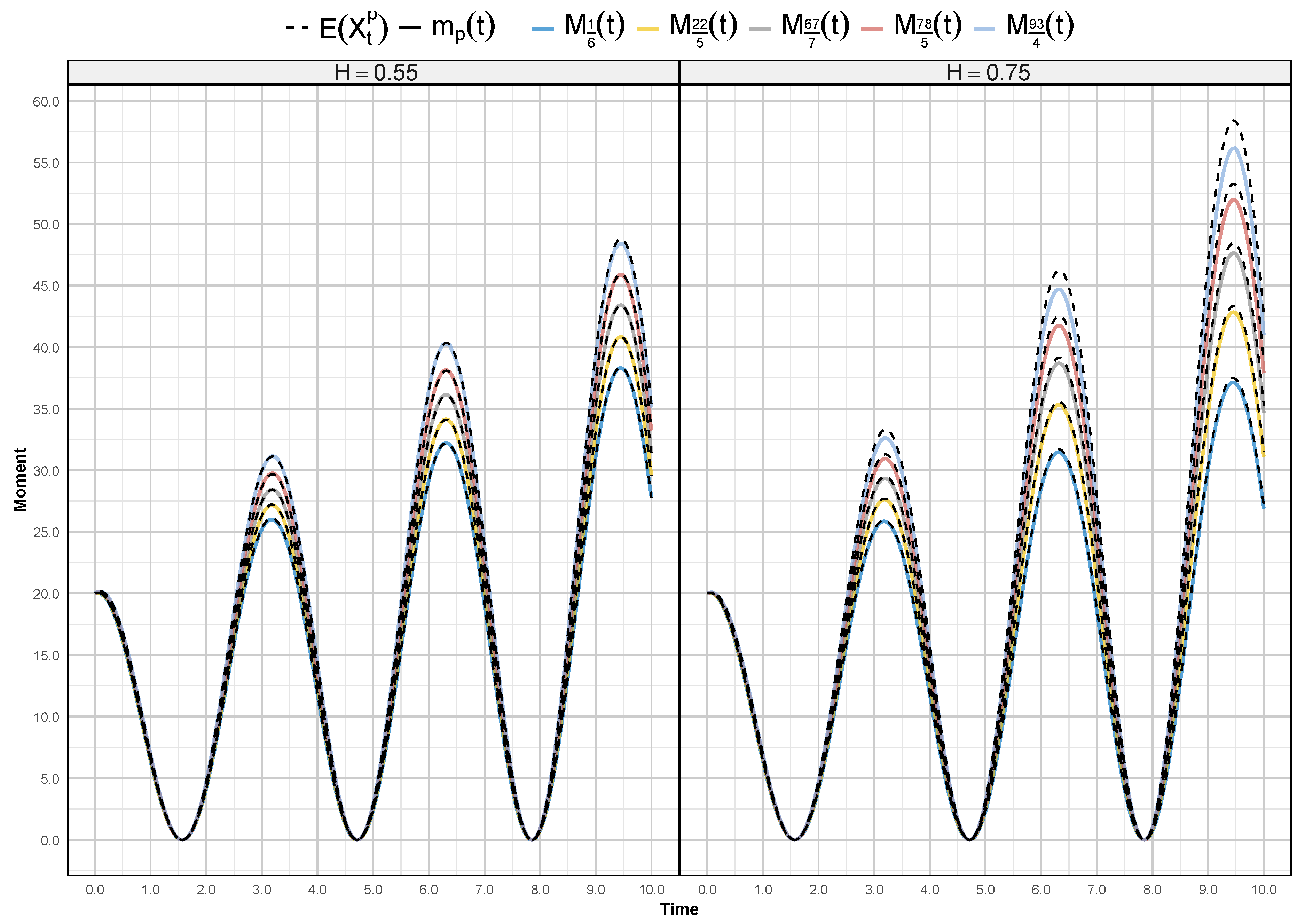
4.1. Linear Time-Dependent Function

As a numerical example for evaluating both fractional and higher integer-order moments, we examine the following process. For this example, the parameters are set as

$$\alpha =-{\displaystyle \frac{1}{2}},\beta =14,\gamma =6,g\left(t\right)=2t+1,\mathrm{and}k=0,$$

where

$$g^{\left(0\right)}\left(t\right)=2t+1\ne 0\mathrm{for}\mathrm{all}t\ge 0.$$

We then consider the following fractional SDE

$$\left\{\begin{array}{c}\mathrm{d}{X}_t=\left(-{\displaystyle \frac{1}{2t+1}}{X}_t+{\displaystyle \frac{14}{\sqrt{2t+1}}}\right)dt+{\displaystyle \frac{6}{\sqrt{2t+1}}}\mathrm{d}{W}_t^H\hfill \\ X_0=30,t\in [0,5]\hfill \end{array}\right.$$

(21)

from (5), it is known that for all $p\ge 0$, the $p^{\mathrm{th}}$ moments of the solution to (21) are given by

$$\mathbb{E}\left(X_t^p\right)=\left\{\begin{array}{cc}{30}^p\hfill & \mathrm{if}t=0\hfill \\ 2^{-\frac{p}{2}}{\left(-6\mathrm{i}\sqrt{{\displaystyle \frac{t^{2H}}{2t+1}}}\right)}^p{\mathcal{H}}_p\left({\displaystyle \frac{\mathrm{i}\sqrt{2}\left(7t+15\right)}{6t^H}}\right)\hfill & \mathrm{if}t>0\hfill \end{array}\right.$$

In Figure 1, we display a visual comparison between the moments obtained via the Monte Carlo simulation $m_p\left(t\right)$ (represented by continuous lines) and the exact values $\mathbb{E}\left(X_t^p\right)$ (represented by dashed lines). This comparison covers both fractional and higher integer-order moments, with orders p chosen from the set $\left\{{\displaystyle \frac{l}{2}}:l=1,\dots ,10\right\}$, over the time interval $t\in [0,5]$.

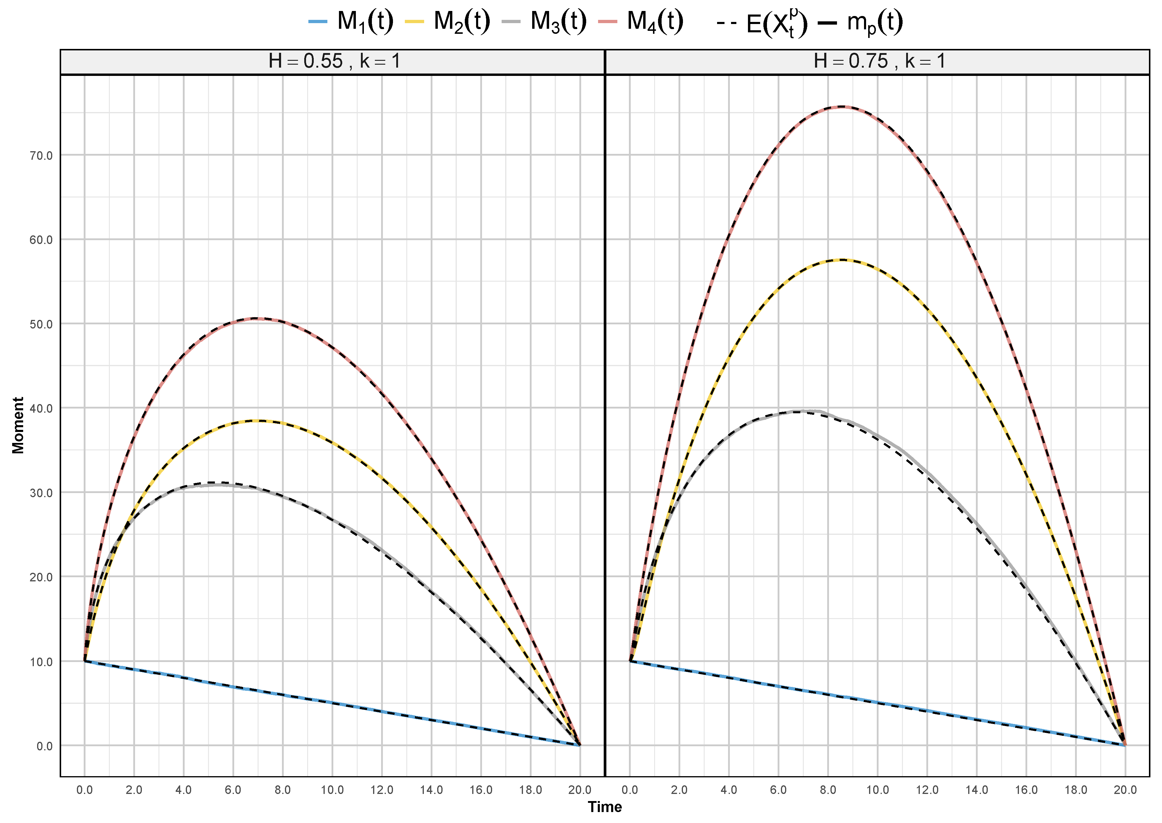
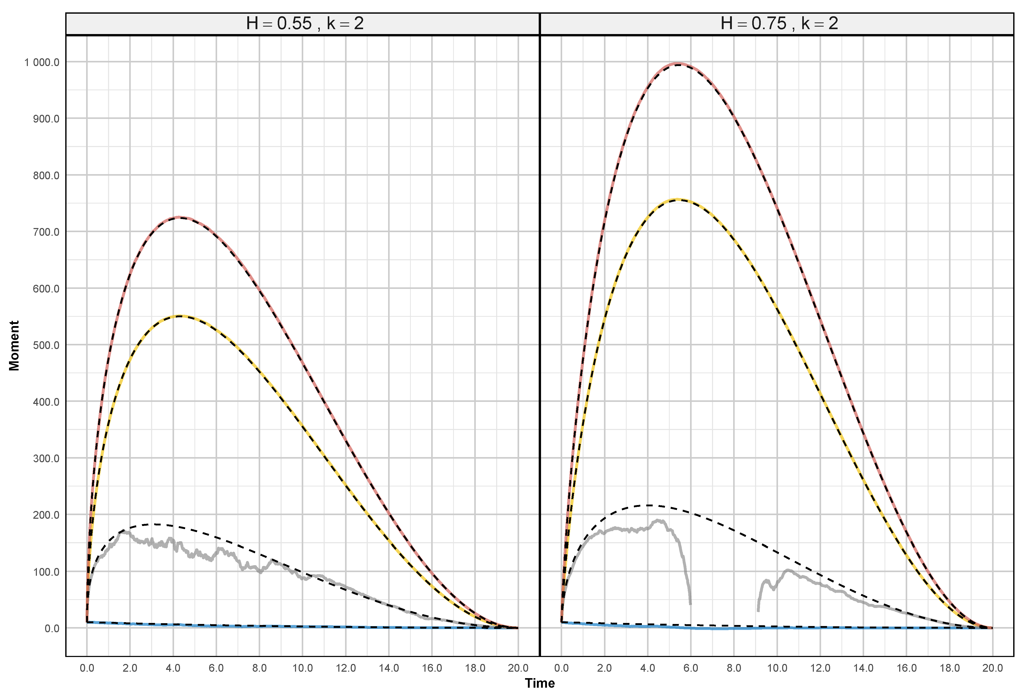
4.2. Non-Linear Time-Dependent Function

In this example, we are interested only in fractional moments. Consider a more complex fractional SDE

$$g\left(t\right)=cos\left(t+\pi \right)\mathrm{and}k=4,\mathrm{where}{g}^{\left(4\right)}\left(t\right)=cos\left(t+\pi \right)$$

and with the parameters $\alpha =\beta =\gamma =2$. Hence, the model under consideration is

$$\left\{\begin{array}{c}\mathrm{d}{X}_t=-2\left(tan\left(t+\pi \right)X_t-{cos}^2\left(t+\pi \right)\right)dt+2{cos}^2\left(t+\pi \right)\mathrm{d}{W}_t^H\hfill \\ X_0=20,t\in [0,10]\hfill \end{array}\right.$$

(22)

Following Equation (15), for all $p\ge 0$, the moments of the solution to (22) are given by

$$\mathbb{E}\left(X_t^p\right)={\displaystyle \frac{{\left({cos}^2(t+\pi )(20+2t)\right)}^p}{2\sqrt{\pi }}}\sum _{j=0}^{\lfloor p\rfloor }\left({\displaystyle \genfrac{}{}{0pt}{}{p}{j}}\right)\left(1+{(-1)}^j\right)\mathrm{\Gamma }\left({\displaystyle \frac{1+j}{2}}\right){\left({\displaystyle \frac{\sqrt{2}}{10+t}}\right)}^j{t}^{jH}$$

Figure 2 presents the Monte Carlo simulation results, computed using (15), for the fractional moments corresponding to $p=\left\{{\displaystyle \frac{1}{6}},{\displaystyle \frac{22}{5}},{\displaystyle \frac{67}{7}},{\displaystyle \frac{78}{5}},{\displaystyle \frac{93}{4}}\right\}$; over the time interval $t\in [0,10]$. Notice that the same results are obtained when using Formula (5).

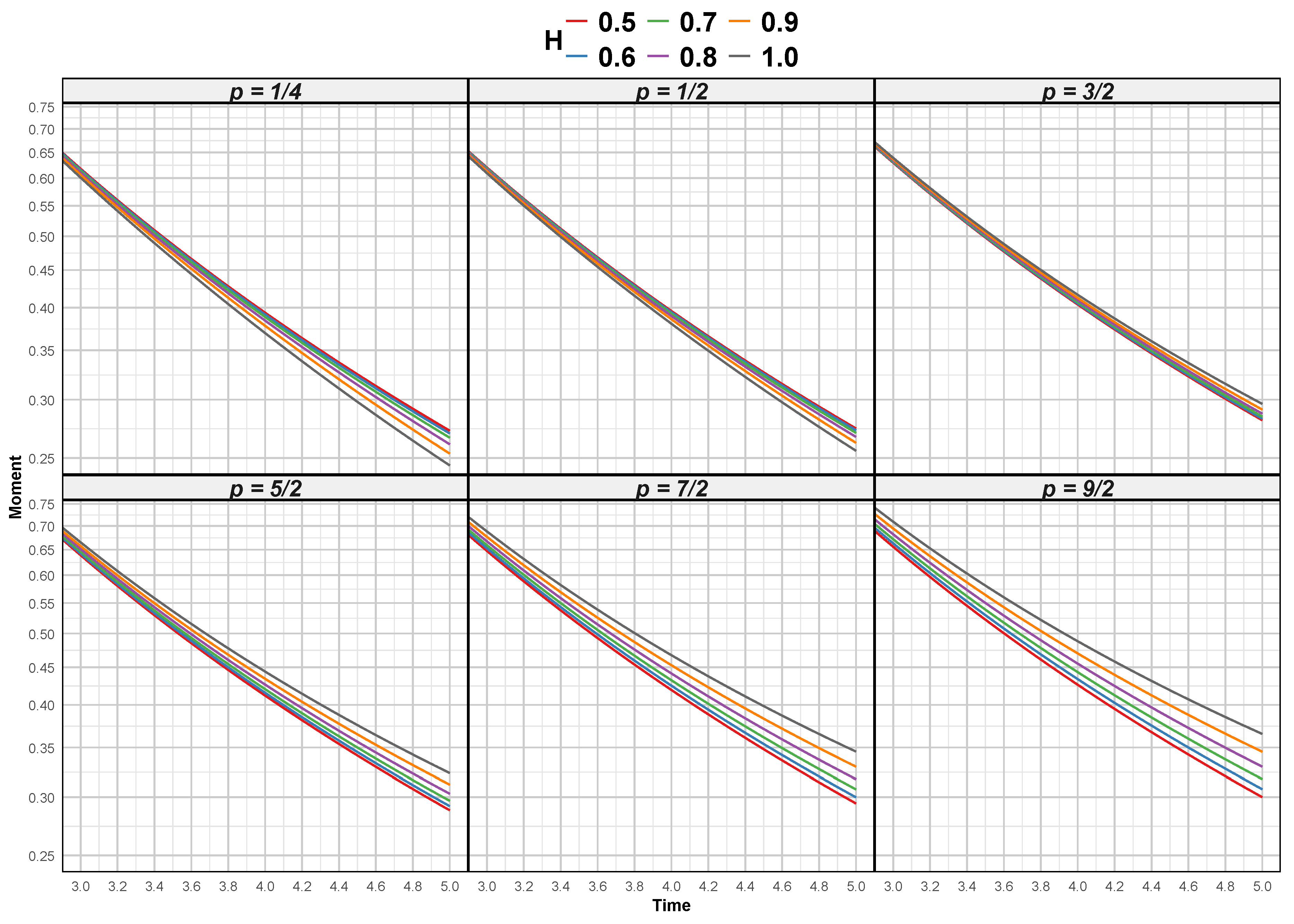
4.3. Fractional Brownian Bridge Process

In this example, we consider the parameters $\alpha =-1$, $\beta =0$, $\gamma =1$ and the function $g\left(t\right)$ is defined by

$$g^{\left(k\right)}\left(t\right)=\left\{\begin{array}{cc}ln(t-20)\hfill & \mathrm{if}k=0\hfill \\ {(-1)}^{k-1}{\displaystyle \frac{\mathrm{\Gamma }\left(k\right)}{{(t-20)}^k}}\hfill & \mathrm{if}k=1,2,3,\cdots \hfill \end{array}\right.$$

for any $k\in {\mathbb{N}}^{+}$, we obtain fractional Brownian bridge process

$$\left\{\begin{array}{c}\mathrm{d}{X}_t={\displaystyle \frac{k}{t-20}}{X}_{t}dt+{\displaystyle \frac{{\left(t-20\right)}^k}{{(-1)}^{k-1}\mathrm{\Gamma }\left(k\right)}}\mathrm{d}{W}_t^H\hfill \\ X_0=10,t\in [0,20]\hfill \end{array}\right.$$

(23)

From (5), for every $p>0$, the exact moments of (23) are given by

$$\mathbb{E}\left(X_t^p\right)=\left\{\begin{array}{cc}{10}^p\hfill & \mathrm{if}t=0\hfill \\ 2^{-{\displaystyle \frac{p}{2}}}{\left({\displaystyle \frac{-\mathrm{i}{\left(t-20\right)}^k{t}^H}{{\left(-1\right)}^{k-1}\mathrm{\Gamma }\left(k\right)}}\right)}^p{\mathcal{H}}_p\left({\displaystyle \frac{10\mathrm{i}{\left(-1\right)}^{k-1}\mathrm{\Gamma }\left(k\right)}{\sqrt{2}{(-20)}^k{t}^H}}\right)\hfill & \mathrm{if}t>0\hfill \end{array}\right.$$

As illustrated in Figure 3, the continuous lines exhibit rough and irregular behavior due to approximation errors in the simulated sample paths, whereas the dashed lines form smooth curves since they represent the exact high integer-order moment values. By computing the moments up to a sufficiently high order, we can gain insights into the statistical properties of (23), such as its mean, variance, skewness, and kurtosis. To illustrate, using the last expression for $p=\{1,2,3,4\}$ and $k\in {\mathbb{N}}^{+}$, we explicitly obtain the first, second, third, and fourth moments.

$$\begin{array}{cc}\mathbb{E}\left(X_t\right)\hfill & =10{\left(-1\right)}^{-k}{\left(-1+{\displaystyle \frac{t}{20}}\right)}^k\hfill \\ \mathbb{E}\left(X_t^2\right)\hfill & ={\left(-1\right)}^{-2k}{\left(-1+{\displaystyle \frac{t}{20}}\right)}^{2k}\left(100+{\displaystyle \frac{{20}^{2k}}{\mathrm{\Gamma }{\left(k\right)}^2}}\times t^{2H}\right)\hfill \\ \mathbb{E}\left(X_t^3\right)\hfill & =10{\left(-1\right)}^{-3k}{\left(-1+{\displaystyle \frac{t}{20}}\right)}^{3k}\left(100+3\times {\displaystyle \frac{{20}^{2k}}{\mathrm{\Gamma }{\left(k\right)}^2}}\times t^{2H}\right)\hfill \\ \mathbb{E}\left(X_t^4\right)\hfill & ={\left(-1\right)}^{-4k}{\left(-1+{\displaystyle \frac{t}{20}}\right)}^{4k}\left(10000+600\times {\displaystyle \frac{{20}^{2k}}{\mathrm{\Gamma }{\left(k\right)}^2}}\times t^{2H}+3\times {\displaystyle \frac{{20}^{4k}}{\mathrm{\Gamma }{\left(k\right)}^4}}\times t^{4H}\right)\hfill \end{array}$$

These explicit expressions not only enable us to calculate the higher-order moments directly but also allow us to derive the variance in an analytical manner. In particular, the variance, defined as $\mathbb{V}\mathrm{ar}\left(X_t\right)=\mathbb{E}\left(X_t^2\right)-{\left[\mathbb{E}\left(X_t\right)\right]}^2$, can be determined directly from the first and second moments.

$$\mathbb{V}\mathrm{ar}\left(X_t\right)={\displaystyle \frac{{\left(-1\right)}^{-2k}}{\mathrm{\Gamma }{\left(k\right)}^2}}{\left(-20+t\right)}^{2k}{t}^{2H}$$

This analytic form provides precise insights into the central tendency and dispersion of the process, thereby facilitating a rigorous assessment of its distributional characteristics. Moreover, with the availability of closed-form expressions for the moments, one can readily analyze the impact of long-range dependence and other parameters on the overall behavior of the stochastic process, further enhancing both theoretical understanding and practical applications.

4.4. Fractional Ornstein–Uhlenbeck Process

Let us consider a particle moving in a viscoelastic medium (e.g., a polymer gel or cellular cytoplasm). The medium’s mechanical memory leads to anomalous diffusion, which can be modeled by a SDE with fractional Brownian motion (fBm). The model captures both the time-dependent friction and the long-term memory ($H>1/2$). We use Equation (1) with the following parameters:

• Function: $g\left(t\right)=t+1$, with $k=0\Rightarrow g^{\left(0\right)}\left(t\right)=t+1$.
• Parameters: $\alpha =-2(\mathrm{mean}\mathrm{reversion})$, $\beta =0(\mathrm{no}\mathrm{external}\mathrm{drift})$, $\gamma =1\left(\mathrm{volatility}\right)$, $H=0.55(\mathrm{long}\mathrm{memory})$.

$$\left\{\begin{array}{c}\mathrm{d}{X}_t=-{\displaystyle \frac{2}{t+1}}{X}_{t}dt+{\displaystyle \frac{1}{{\left(t+1\right)}^2}}\mathrm{d}{W}_t^H\hfill \\ X_0=10,t\in [0,5]\hfill \end{array}\right.$$

(24)

from (5), for all $p\ge 0$, the $p\mathrm{th}$ moments of (24) are given by

$$\mathbb{E}\left(X_t^p\right)=\left\{\begin{array}{cc}{10}^p\hfill & \mathrm{if}t=0\hfill \\ 2^{-{\displaystyle \frac{p}{2}}}{\left(-\mathrm{i}\sqrt{{\displaystyle \frac{t^{2H}}{{(t+1)}^4}}}\right)}^p{\mathcal{H}}_p\left(5\mathrm{i}\sqrt{{\displaystyle \frac{2}{t^{2H}}}}\right)\hfill & \mathrm{if}t>0\hfill \end{array}\right.$$

The results obtained in this example underscore the unique insights offered by fractional moments when analyzing complex stochastic processes driven by fractional Brownian motion. In our case, the model describes a particle moving in a viscoelastic medium—a scenario where the medium’s memory effects result in anomalous diffusion. Unlike traditional moments that provide measures for dispersion, skewness, and kurtosis, fractional moments capture the behavior of the process at non-integer orders, offering a more delicate probe into its dynamics.

By explicitly deriving the fractional moments for orders such as $p=\left\{1/4,1/2,\dots \right\}$, we demonstrate that even though these moments do not directly yield classical measures of dispersion or asymmetry, they still provide valuable information about the underlying distribution. They help reveal the influence of the long memory (as characterized by the Hurst index $H=0.55$) on the process, particularly how the interplay between the time-dependent drift and diffusion components shapes the evolution of the system. Moreover, the close agreement between the Monte Carlo simulation results and the analytically derived fractional moments—as illustrated in Figure 4 on a logarithmic scale—reinforces the robustness of the proposed method. In summary, while fractional moments may not directly allow the computation of dispersion, skewness, and kurtosis, they serve as an indispensable tool for characterizing the complex statistical properties of anomalously diffusing systems, thereby enhancing our overall understanding of such processes.

In the Figure 5, we illustrated the evolution of fractional-order moments associated with the fractional Ornstein–Uhlenbeck (fOU) process for various values of the Hurst exponent $H=\left\{0.5,0.6,0.7,0.8,0.9,1.0\right\}$ and different orders $p=\left\{1/4,1/2,3/2,5/2,7/2,9/2\right\}$. This visualization highlights the influence of long-range dependence on the statistical properties of the process over time. The results indicate that the moments exhibit a strong dependency on both H and p, revealing distinct scaling behaviors. Specifically, for smaller values of H, the process exhibits a faster decay in moment magnitudes, indicating weaker persistence and stronger mean reversion. Conversely, higher values of H correspond to a slower decay, reflecting stronger long-memory effects characteristic of the fOU process. Additionally, increasing the order p amplifies these differences, particularly in the tail behavior of the process. This is evident in the non-linearity observed in moment growth, which is more pronounced for larger H. The curvature of the moment trajectories suggests that higher-order moments capture subtle deviations from Gaussianity, influenced by the underlying memory structure.

Overall, these results provide a deeper insight into the impact of the Hurst exponent on the statistical moments of the fOU process. The Figure 5 serves as empirical evidence of how long-range dependence modulates the higher-order dynamics of the process, emphasizing the need for accurate moment estimation when characterizing such systems.

Table 1. Exact fractional moments $\mathbb{E}\left(X_t^p\right)$ of model (24), computed for various fractional orders p and Hurst parameters $H\in (0.5,1.0)$, evaluated at time points $t=\{0,1,2,3,4,5\}$.

	p	H	Time
			0.0	1.0	2.0	3.0	4.0	5.0
$\mathbb{E}\left(X_t^p\right)$	${\displaystyle \frac{1}{4}}$	0.5	10.0000	2.4905	1.1026	0.6177	0.3937	0.2722
		0.6	10.0000	2.4905	1.1013	0.6158	0.3915	0.2699
		0.7	10.0000	2.4905	1.0998	0.6134	0.3885	0.2663
		0.8	10.0000	2.4905	1.0980	0.6103	0.3841	0.2609
		0.9	10.0000	2.4905	1.0960	0.6063	0.3779	0.2534
		1.0	10.0000	2.4905	1.0936	0.6008	0.3694	0.2442
	${\displaystyle \frac{1}{2}}$	0.5	10.0000	2.4937	1.1055	0.6202	0.3958	0.2741
		0.6	10.0000	2.4937	1.1046	0.6189	0.3944	0.2726
		0.7	10.0000	2.4937	1.1036	0.6174	0.3925	0.2704
		0.8	10.0000	2.4937	1.1024	0.6154	0.3897	0.2670
		0.9	10.0000	2.4937	1.1011	0.6128	0.3858	0.2621
		1.0	10.0000	2.4937	1.0996	0.6093	0.3804	0.2556
	${\displaystyle \frac{3}{2}}$	0.5	10.0000	2.5063	1.1167	0.6297	0.4040	0.2813
		0.6	10.0000	2.5063	1.1175	0.6309	0.4053	0.2826
		0.7	10.0000	2.5063	1.1185	0.6323	0.4070	0.2845
		0.8	10.0000	2.5063	1.1196	0.6341	0.4093	0.2871
		0.9	10.0000	2.5063	1.1208	0.6364	0.4124	0.2908
		1.0	10.0000	2.5063	1.1223	0.6393	0.4165	0.2960
	${\displaystyle \frac{5}{2}}$	0.5	10.0000	2.5186	1.1276	0.6388	0.4117	0.2879
		0.6	10.0000	2.5186	1.1300	0.6421	0.4153	0.2916
		0.7	10.0000	2.5186	1.1327	0.6462	0.4200	0.2965
		0.8	10.0000	2.5186	1.1359	0.6513	0.4261	0.3031
		0.9	10.0000	2.5186	1.1395	0.6574	0.4339	0.3118
		1.0	10.0000	2.5186	1.1436	0.6650	0.4438	0.3232
	${\displaystyle \frac{7}{2}}$	0.5	10.0000	2.5542	1.1758	0.6672	0.4295	0.3036
		0.6	10.0000	2.5542	1.1784	0.6710	0.4336	0.3080
		0.7	10.0000	2.5542	1.1814	0.6753	0.4385	0.3134
		0.8	10.0000	2.5542	1.1850	0.6804	0.4443	0.3199
		0.9	10.0000	2.5542	1.1891	0.6864	0.4511	0.3276
		1.0	10.0000	2.5542	1.1937	0.6933	0.4590	0.3366
	${\displaystyle \frac{9}{2}}$	0.5	10.0000	2.5664	1.1862	0.6755	0.4363	0.3094
		0.6	10.0000	2.5664	1.1890	0.6795	0.4407	0.3141
		0.7	10.0000	2.5664	1.1922	0.6839	0.4459	0.3197
		0.8	10.0000	2.5664	1.1960	0.6892	0.4519	0.3265
		0.9	10.0000	2.5664	1.2003	0.6955	0.4589	0.3345
		1.0	10.0000	2.5664	1.2051	0.7027	0.4669	0.3438

presents the exact fractional moments of (24), computed for various values of the fractional order p and Hurst parameter H, evaluated at different time points t. The results highlight the influence of the long-range dependence parameter H on the evolution of fractional moments.

The analysis of fractional moments of (24) as a function of the Hurst parameter H reveals distinct trends depending on the order p as shown in Figure 6. When $p<1$, the moments exhibit a decreasing behavior as H increases, indicating that higher long-range dependencies in the process lead to a reduction in expected values of fractional powers. This suggests that for small moment orders, stronger memory effects (higher H) contribute to a more stable and less dispersed process. Conversely, when $p>1$, the moments show a monotonic increase with H, highlighting the fact that long memory amplifies large fluctuations in the process. Interestingly, for $p=1$, the moments remain approximately stable across different values of H, suggesting an equilibrium point where the effects of long-range dependence do not significantly alter the mean behavior of the process. These contrasting behaviors underline the non-trivial interaction between fractional moment orders and memory effects, which has important implications for understanding the statistical properties of stochastic processes driven by fractional Brownian motion.

5. Conclusions and Perspectives

This study has provided a comprehensive analysis of fractional and higher integer-order moments in stochastic processes governed by stochastic differential equations (SDEs) driven by fractional Brownian motion (fBm). By leveraging Wick–Itô calculus and Hermite polynomials, explicit closed-form expressions for these moments were derived, offering a more tractable and efficient alternative to classical approaches. The results reveal a fundamental interaction between the moment order p and the Hurst parameter H, illustrating three distinct regimes: a decreasing trend of moments for $p<1$ as H increases, a stable behavior for $p=1$, and an increasing trend for $p>1$. These findings underscore the profound influence of long-memory effects on the statistical properties of fractional processes, particularly in their higher-order moments, which are crucial for understanding the dynamics of complex systems.

The numerical validation, conducted through Monte Carlo simulations, confirms the robustness of the theoretical results, demonstrating their accuracy in capturing the underlying stochastic dynamics. The ability to explicitly characterize the moments of fractional processes opens new perspectives in both theoretical and applied domains. In mathematical finance, these results provide a valuable tool for modeling asset price dynamics in markets exhibiting long-range dependence, improving volatility estimation and risk management strategies. In statistical inference, the derived moment expressions establish a solid foundation for efficient parameter estimation in fractional models, enhancing the accuracy of empirical studies. Similarly, in physics and engineering, the proposed framework can be applied to describe anomalous diffusion processes, turbulence models, and a variety of physical systems where memory effects play a crucial role. These insights contribute to a deeper understanding of the mechanisms governing non-Markovian dynamics and their impact on real-world phenomena.

Despite the significant theoretical advancements, several challenges remain. One limitation of the current approach is its reliance on linear fractional SDEs, which may not fully capture the complexity of real-world systems exhibiting non-linearity and strong non-Gaussian behavior. A natural extension of the present work is to move beyond the linear class of fractional SDEs and investigate genuinely non-linear dynamics. In such cases, the Gaussian change of variable and the Hermite-based moment closure adopted here no longer yield a finite hierarchy of moment equations. Complementary tools are therefore required: perturbative expansions around the linear reference case, moment-closure approximations, chaos expansions grounded in Malliavin calculus, or high-order numerical schemes that combine spectral methods with Monte Carlo sampling. Developing a systematic framework along these lines will be a central focus of our future research.

Additionally, while this study focuses on one-dimensional processes, extending these results to multidimensional fractional SDEs would allow for a deeper investigation of interacting systems with long-memory characteristics, such as coupled financial assets, multi-component diffusion models, or climate variables. Furthermore, integrating these findings into machine learning frameworks could enhance predictive modeling for time series exhibiting non-Markovian behavior. The exploration of fractional moment-based techniques in real-world applications remains an exciting avenue for further investigation, with potential implications in finance, climatology, biophysics, and beyond.

In summary, this work provides a solid mathematical foundation for the study of fractional moments in stochastic processes, bridging theoretical developments with practical applications. The interplay between long-memory effects and higher-order moments offers valuable insights into a wide range of complex systems, setting the stage for further advancements in both theoretical and applied research.

References

1. Klebaner, F.C. Introduction to Stochastic Calculus with Applications, 2nd ed.; Imperial College Press: London, UK, 2005. [Google Scholar] [CrossRef]
2. Allen, E. Mathematical Modelling: Theory and Applications. In Modeling with Itô Stochastic Differential Equations, 1st ed.; Springer: Berlin/Heidelberg, Germany, 2007; Volume 22. [Google Scholar] [CrossRef]
3. Jedrzejewski, F. Modèles Aléatoires et Physique Probabiliste; Springer: Berlin/Heidelberg, Germany, 2009. [Google Scholar] [CrossRef]
4. Freidlin, M.I.; Wentzell, A.D. Grundlehren der mathematischen Wissenschaften. In Random Perturbations of Dynamical Systems; Springer: Berlin/Heidelberg, Germany, 2012; Volume 260. [Google Scholar] [CrossRef]
5. Živorad, T.; Sandev, T.; Metzler, R.; Dubbeldam, J. Generalized space–time fractional diffusion equation with composite fractional time derivative. Phys. A Stat. Mech. Its Appl. 2012, 391, 2527–2542. [Google Scholar] [CrossRef]
6. Lange, K. Statistics for Biology and Health. In Mathematical and Statistical Methods for Genetic Analysis, 2nd ed.; Springer: Berlin/Heidelberg, Germany, 2002. [Google Scholar] [CrossRef]
7. Han, X.; Kloeden, P.E. Probability Theory and Stochastic Modelling. In Random Ordinary Differential Equations and Their Numerical Solution, 1st ed.; Springer: Berlin/Heidelberg, Germany, 2017; Volume 85. [Google Scholar] [CrossRef]
8. Panik, M.J. Stochastic Differential Equations: An Introduction with Applications in Population Dynamics Modeling; John Wiley & Sons: Hoboken, NJ, USA, 2017. [Google Scholar] [CrossRef]
9. Atangana, A.; İgret Araz, S. Industrial and Applied Mathematics. In Fractional Stochastic Differential Equations: Applications to Covid-19 Modeling, 1st ed.; Springer Nature: Singapore, 2022. [Google Scholar] [CrossRef]
10. Rolski, T.; Schmidli, H.; Schmidt, V.; Teugels, J. Stochastic Processes for Insurance and Finance; John Wiley & Sons: Hoboken, NJ, USA, 2008. [Google Scholar] [CrossRef]
11. Iacus, S.M. Option Pricing and Estimation of Financial Models with R; John Wiley & Sons: Hoboken, NJ, USA, 2011. [Google Scholar] [CrossRef]
12. Nguyen Tien, D. Fractional stochastic differential equations with applications to finance. J. Math. Anal. Appl. 2013, 397, 334–348. [Google Scholar] [CrossRef]
13. Rostek, S.; Schöbel, R. A note on the use of fractional Brownian motion for financial modeling. Econ. Model. 2013, 30, 30–35. [Google Scholar] [CrossRef]
14. Mackevicius, V. Stochastic Models of Financial Mathematics, 1st ed.; Elsevier: Amsterdam, The Netherlands, 2016. [Google Scholar] [CrossRef]
15. Primak, S.; Kontorovich, V.; Lyandres, V. Stochastic Methods and Their Applications to Communications, Stochastic Differential Equations Approach; John Wiley & Sons: Hoboken, NJ, USA, 2004. [Google Scholar] [CrossRef]
16. Henderson, D.; Plaschko, P. Stochastic Differential Equations in Science and Engineering; World Scientific: Singapore, 2006. [Google Scholar] [CrossRef]
17. Kolmogorov, A.N. Wienersche spiralen und einige andere interessante kurven in hilbertscen raum, cr (doklady). Acad. Sci. URSS 1940, 26, 115–118. [Google Scholar]
18. Mandelbrot, B.B.; Ness, J.W.V. Fractional Brownian Motions, Fractional Noises and Applications. SIAM Rev. 1968, 10, 422–437. [Google Scholar] [CrossRef]
19. Maslowski, B.; Nualart, D. Evolution equations driven by a fractional Brownian motion. J. Funct. Anal. 2003, 202, 277–305. [Google Scholar] [CrossRef]
20. Mishura, Y.S. Stochastic Calculus for Fractional Brownian Motion and Related Processes, 1st ed.; Lecture Notes in Mathematics; Springer: Berlin/Heidelberg, Germany, 2008. [Google Scholar] [CrossRef]
21. Ascione, G.; Mishura, Y.; Pirozzi, E. Fractional Deterministic and Stochastic Calculus; De Gruyter: Berlin, Germany; Boston, MA, USA, 2024. [Google Scholar] [CrossRef]
22. Ullah, R.; Farooq, M.; Faizullah, F.; Alghafli, M.A.; Mlaiki, N. Fractional stochastic functional differential equations with non-Lipschitz condition. AIMS Math. 2025, 10, 7127–7143. [Google Scholar] [CrossRef]
23. Bishwal, J.P.N. Parameter Estimation in Stochastic Differential Equations, 1st ed.; Lecture Notes in Mathematics; Springer: Berlin/Heidelberg, Germany, 2008. [Google Scholar] [CrossRef]
24. Bishwal, J.P.N. Parameter Estimation in Stochastic Volatility Models, 1st ed.; Springer: Cham, Switzerland, 2012. [Google Scholar] [CrossRef]
25. Rao, B.P. Statistical Inference for Fractional Diffusion Processes, 1st ed.; John Wiley & Sons, Ltd.: Hoboken, NJ, USA, 2010. [Google Scholar] [CrossRef]
26. Risken, H. The Fokker-Planck Equation: Methods of Solution and Applications, 2nd ed.; Springer Series in Synergetics; Springer: Berlin/Heidelberg, Germany, 1996; Volume 18. [Google Scholar] [CrossRef]
27. Živorad, T.; Ralf, M.; Stefan, G. Fractional characteristic functions, and a fractional calculus approach for moments of random variables. Fract. Calc. Appl. Anal. 2022, 25, 1307–1323. [Google Scholar] [CrossRef]
28. Cottone, G.; Di Paola, M.; Metzler, R. Fractional calculus approach to the statistical characterization of random variables and vectors. Phys. A Stat. Mech. Its Appl. 2010, 389, 909–920. [Google Scholar] [CrossRef]
29. Graham, C.; Talay, D. Stochastic Modelling and Applied Probability. In Stochastic Simulation and Monte Carlo Methods: Mathematical Foundations of Stochastic Simulation, 1st ed.; Springer: Berlin/Heidelberg, Germany, 2013; Volume 68. [Google Scholar] [CrossRef]
30. Thomopoulos, N.T. Essentials of Monte Carlo Simulation: Statistical Methods for Building Simulation Models, 1st ed.; Springer: Berlin/Heidelberg, Germany, 2013. [Google Scholar] [CrossRef]
31. Li, M. PSD and Cross-PSD of Responses of Seven Classes of Fractional Vibrations Driven by fGn, fBm, Fractional OU Process, and von Kármán Process. Symmetry 2024, 16, 635. [Google Scholar] [CrossRef]
32. Russo, F.; Vallois, P. Stochastic calculus with respect to continuous finite quadratic variation processes. Stochastics Stoch. Rep. 2000, 70, 1–40. [Google Scholar] [CrossRef]
33. Nualart, D.; Răşcanu, A. Differential equations driven by fractional Brownian motion. Collect. Math. 2002, 53, 55–81. [Google Scholar]
34. Guerra, J.; Nualart, D. Stochastic Differential Equations Driven by Fractional Brownian Motion and Standard Brownian Motion. Stoch. Anal. Appl. 2008, 26, 1053–1075. [Google Scholar] [CrossRef]
35. Merton, R.C. Theory of Rational Option Pricing. Bell J. Econ. Manag. Sci. 1973, 4, 141–183. [Google Scholar] [CrossRef]
36. Cheridito, P.; Kawaguchi, H.; Maejima, M. Fractional Ornstein-Uhlenbeck processes. Electron. J. Probab. 2003, 8, 1–14. [Google Scholar] [CrossRef]
37. Guidoum, A.C.; Boukhetala, K. Exact higher-order moments for linear non-homogeneous stochastic differential equation. Model Assist. Stat. Appl. 2023, 18, 321–329. [Google Scholar] [CrossRef]
38. Decreusefond, L.; Üstünel, A.S. Stochastic Analysis of the Fractional Brownian Motion. Potential Anal. 2001, 10, 177–214. [Google Scholar] [CrossRef]
39. Alòs, E.; Mazet, O.; Nualart, D. Stochastic Calculus with Respect to Gaussian Processes. Ann. Probab. 2001, 29, 766–801. [Google Scholar] [CrossRef]
40. Bender, C. An Itô formula for generalized functionals of a fractional Brownian motion with arbitrary Hurst parameter. Stoch. Process. Their Appl. 2003, 104, 81–106. [Google Scholar] [CrossRef]
41. Olver, F.W.; Lozier, D.W.; Boisvert, R.F.; Clark, C.W. NIST Handbook of Mathematical Functions, 1st ed.; Cambridge University Press: New York, NY, USA, 2010. [Google Scholar]
42. Willink, R. Normal moments and Hermite polynomials. Stat. Probab. Lett. 2005, 73, 271–275. [Google Scholar] [CrossRef]
43. Winkelbauer, A. Moments and Absolute Moments of the Normal Distribution. arXiv 2014. [Google Scholar] [CrossRef]
44. R Core Team. R: A Language and Environment for Statistical Computing; R Foundation for Statistical Computing: Vienna, Austria, 2025; Available online: https://www.r-project.org/ (accessed on 15 March 2025).
45. Guidoum, A.C.; Boukhetala, K. Performing Parallel Monte Carlo and Moment Equations Methods for Itô and Stratonovich Stochastic Differential Systems: R Package Sim.DiffProc. J. Stat. Softw. 2020, 96, 1–82. [Google Scholar] [CrossRef]
46. Brouste, A.; Fukasawa, M.; Hino, H.; Iacus, S.M.; Kamatani, K.; Koike, Y.; Masuda, H.; Nomura, R.; Ogihara, T.; Shimuzu, Y.; et al. The yuima Project: A Computational Framework for Simulation and Inference of Stochastic Differential Equations. J. Stat. Softw. 2014, 57, 1–51. [Google Scholar] [CrossRef]
47. Iacus, S.M.; Yoshida, N. Simulation and Inference for Stochastic Processes with yuima: A Comprehensive R Framework for SDEs and Other Stochastic Processes; Springer: Berlin/Heidelberg, Germany, 2018. [Google Scholar] [CrossRef]
48. Burlon, A. On the numerical solution of fractional differential equations under white noise processes. Probabilistic Eng. Mech. 2023, 73, 103465. [Google Scholar] [CrossRef]
Figure 1. The p th approximate m p ( t ) and exact moments E X t p of (21), where p = l 2 : l = 1 , , 10 . (Left): Hurst index H = 0.55 . (Right): H = 0.75 .
Symmetry 17 00665 g001
Figure 2. The p th approximate m p ( t ) and exact moments E X t p of (22), where p = 1 6 , 22 5 , 67 7 , 78 5 , 93 4 . (Left): Hurst index H = 0.55 . (Right): H = 0.75 .
Symmetry 17 00665 g002
Figure 3. The 1st–4th approximate m p ( t ) and exact moments E X t p of (23) where top k = 1 and bottom k = 2 . (Left): Hurst index H = 0.55 . (Right): H = 0.75 .
Symmetry 17 00665 g003aSymmetry 17 00665 g003b
Figure 4. The p th approximate m p ( t ) and exact moments E X t p of (24), where p = l / 2 : l = 1 , 3 , 5 , 7 , 9 and Hurst index H = 0.55 .
Symmetry 17 00665 g004
Figure 5. Evolution of exact fractional moments E X t p of (24) with various values of the order p and Hurst parameter H.
Symmetry 17 00665 g005
Figure 6. Impact of the Hurst parameter H on exact fractional moments E X t p of (24) with different order p at time t = 5 .
Symmetry 17 00665 g006