An Advanced Adaptive Group Learning Particle Swarm Optimization Algorithm

Abstract

The particle swarm optimization algorithm, known for its swift convergence and minimal parameters, is widely used to solve various complex optimization problems. Despite its merits, it encounters challenges such as susceptibility to premature convergence and reduced search capability in later stages. To improve the optimization performance of the algorithm, this study designs an advanced adaptive Group Learning Particle Swarm Optimization (GLPSO) algorithm based on the concept of symmetry. Firstly, a new coefficient is proposed to enable rapid convergence of the algorithm, allowing the population to quickly converge to the optimal position. By adopting a group learning mechanism, the optimal particles in each group are learned during particle updates; this enhances the diversity of particle learning in the algorithm, improving its global search capability. A novel adaptive perturbation rule is proposed, enabling particles to perform perturbations in a more suitable manner, thereby enhancing the population’s ability to escape local optima. GLPSO is compared with several advanced algorithms on internationally recognized high-dimensional benchmark functions and is also applied to some constrained engineering problems. The results indicate that GLPSO outperforms other improved algorithms on most test problems and provides competitive and high-quality solutions for engineering problems. Overall, GLPSO enhances its optimization capability while maintaining robustness.

1. Introduction

With the rapid development of science and technology, meta-heuristic algorithms play an important role in solving problems in various fields, such as engineering technology [1,2,3], biomedicine [4,5], and information science [6,7,8,9,10]. Traditional optimization methods, such as the gradient descent method [11] and the Newton method [12], face issues like high computational complexity and the tendency to become trapped in local optima when dealing with complex, nonlinear, and multimodal optimization problems, which limits their scope of application. Therefore, researchers continuously explore new optimization algorithms in hopes of addressing these challenges more effectively.

Meta-heuristic algorithms, by abstractly simulating real-world processes and applying diverse search strategies within the search space to explore and update solutions, can address most optimization problems in these fields. For example, the Genetic Algorithm (GA) [13] solves optimization problems by simulating the biological evolution process. The Simulated Annealing algorithm (SA) [14] is based on the principle of the annealing process in physics and prevents the algorithm from falling into local optima by gradually reducing the temperature. Ant Colony Optimization (ACO) [15] simulates the pheromone renewal mechanism in the ant foraging process, enabling effective solutions for complex path planning problems. The Grey Wolf Optimizer (GWO) [16] explores the solution space by mimicking the hunting behavior of wolves in nature. The core idea of particle swarm optimization (PSO) [17] is based on the foraging behavior of birds in nature, finding the optimal solution through information sharing and cooperation among particles.

Different meta-heuristic algorithms are suitable for solving different problems due to their unique advantages. Since the particle swarm optimization (PSO) algorithm was proposed by Kennedy and Eberhart in 1995, it has quickly become a prominent research focus in the optimization field. This is attributed to its straightforward principles, ease of implementation, minimal parameter demands, and swift convergence rate [18]. Although the PSO algorithm has achieved remarkable results in many fields, it still has some shortcomings, such as premature convergence, declining search capability in later stages, sensitivity to parameters, and other issues [19,20,21]. To further improve the performance and applicability of the PSO algorithm, many researchers have proposed enhancements from various perspectives. These improvements include the introduction of new particle update strategies [22,23,24,25], dynamic adjustment of algorithm parameters [26], dynamic regulation of population size [27], and the integration of concepts from other optimization algorithms [28,29,30,31], aiming to improve the algorithm’s convergence speed, enhance its global search ability, and reduce the risk of getting trapped in local optima.

Liang et al. proposed the Comprehensive Learning Particle Swarm Optimizer (CLPSO) algorithm [19], which uses the best historical information from all particles in the group to update particle velocity. This algorithm updates particle information and considers different dimensions independently. The innovative handling of particle dimensions in CLPSO allows it to escape local optima effectively and perform well on high-dimensional problems; however, for general-dimensional problems, its advantages are less pronounced. In high-dimensional cases, the high sensitivity of CLPSO to dimension can lead to a significant increase in the algorithm’s practical complexity and computational load. Modified Particle Swarm Optimization (MPSO) [31] adopts an adaptive updating strategy and introduces both random and mainstream learning strategies, improving the global and individual best learning strategies in PSO and effectively enhancing algorithm performance. However, MPSO still suffers from slow convergence and a tendency to become trapped in local optima. The Elite Archives-Driven Particle Swarm Optimization (EAPSO) [25] establishes an elite archive and uses different update strategies for different particles, updating only a subset of particles. While this approach reduces the computational complexity of the algorithm, it also decreases the convergence speed.

In addition, there are many new perspectives for improving PSO. Sukanta et al. combined an improved Backtracking Search Algorithm (BSA) with PSO to propose a new variant (e-mPSOBSA) for solving global optimization tasks [29]. Li et al. introduced a Pyramid PSO (PPSO) with competitive and cooperative mechanisms to update particle information [32]. Meng et al. proposed a PSO-based single-objective numerical optimization variant (PSO-sono) [33]. EOPSO [34] proposed an elite–ordinary collaborative PSO method that divides particles into elite and ordinary members based on their fitness values.

To address the issues of increasing computational complexity, slow convergence speed, and the tendency to fall into local optima in PSO variants, this paper proposes an adaptive perturbation-based Group Learning Particle Swarm Optimization algorithm, called GLPSO. By preserving the original advantages of the PSO algorithm, it overcomes the shortcomings of slow convergence and susceptibility to local optima, thereby improving the overall performance of the algorithm. The algorithm demonstrates rapid convergence during the initial iteration stage, while the perturbation strategies employed at different stages enhance its global search performance and help avoid local optima. This leads to faster attainment of better optimal solutions and provides new insights for further improvements in optimization problems characterized by multiple local optima. The contributions of this paper are as follows:

• This research utilizes the Latin hypercube sampling and reverse learning mechanisms for population initialization, ensuring that the initial population is evenly distributed across the search space. This approach yields a more advantageous initial population, enhancing the probability of the algorithm finding the global optimal solution during the search process, preventing premature convergence, and improving algorithm stability.
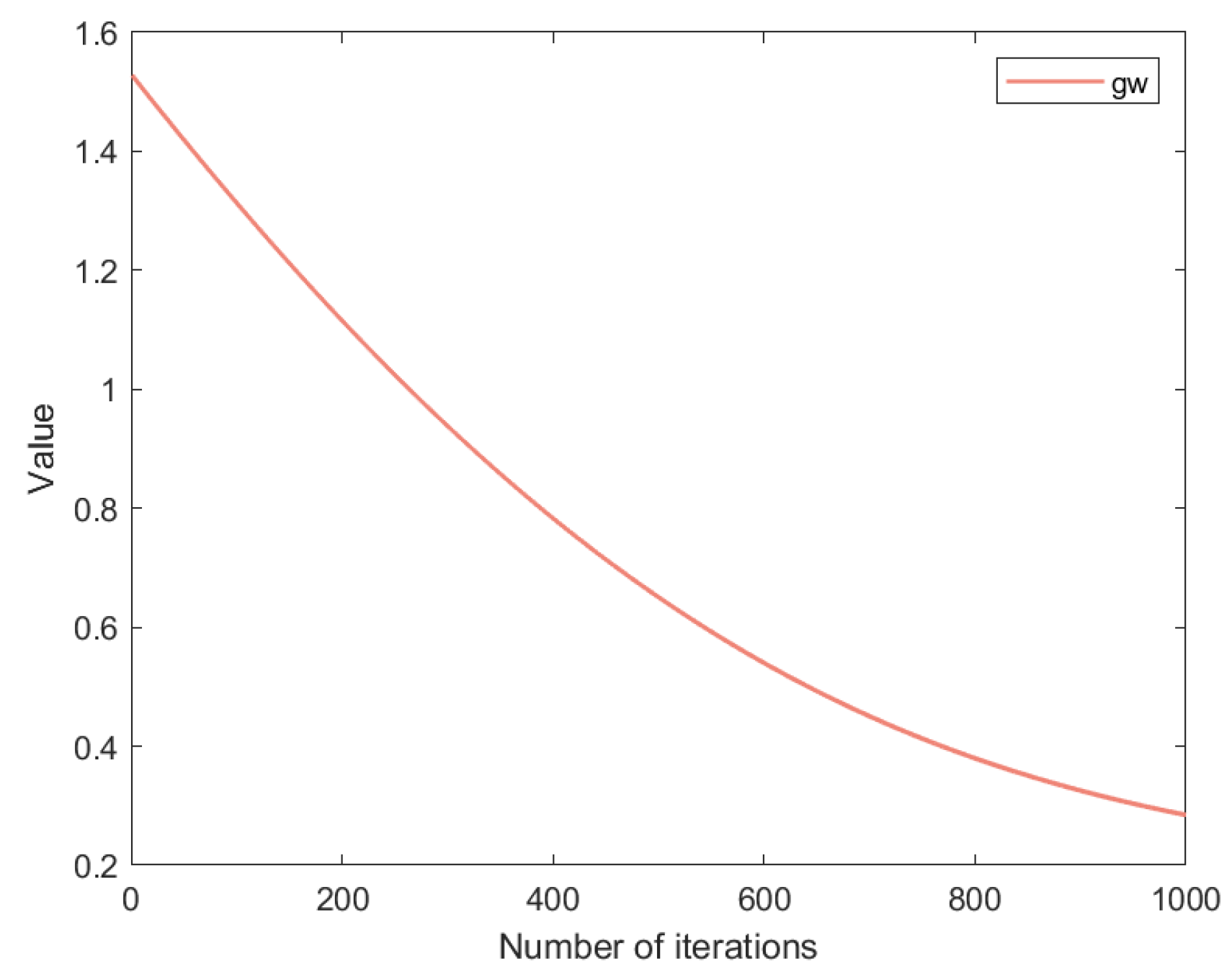
• A new golden sine perturbation coefficient is proposed and applied to the linearly decreasing inertia weight, allowing the algorithm to adaptively explore the search space more effectively during different search phases and enhancing the convergence speed of the algorithm.
• A staged group learning mechanism is proposed. In each iteration, the population is randomly divided into groups to establish a group learning approach, with the number of group members adapting to changes at different stages of the iteration. The velocity update formula is improved, enhancing the diversity of population learning and increasing the algorithm’s global search capability.
• An adaptive Gaussian perturbation strategy is proposed to apply adaptive perturbations to different particle velocities in the group, facilitating particles to escape local optima and more effectively balancing the algorithm’s exploration and exploitation capabilities.

This paper is organized as follows: Section 2 introduces the classical PSO, introduces the concepts of Latin hypercube sampling and opposition-based learning, and presents a Gaussian perturbation. Section 3 proposes an adaptive perturbation-based Group Learning Particle Swarm Optimization (GLPSO) algorithm. Section 4 presents the algorithm settings for the CEC-2017 test functions and analyzes the results. This study provides a detailed performance analysis of the algorithm in Section 5. In Section 6, GLPSO is applied to two engineering problems. Section 7 provides conclusions and outlines future research directions.

2. Basic Concepts

2.1. Classic PSO

PSO abstracts birds as particles by simulating their predatory behavior and utilizes information sharing among individuals in the group. This allows the entire group to search each region through a division of labor, continuously seeking the optimal solution while exploring the search space. The particle update diagram is illustrated in Figure 1.

In the search space, the position of the ith particle at the tth iteration is denoted as $x_i^t$. The velocity of the ith particle at the tth iteration is represented as $v_i^t$. The yellow particle represents the current particle being updated, the red particle represents the next position of the updated particle, and the green particles represent other particles in the population during the tth iteration. The (1) and (2) represent the update rule for the position of the particle in the t + 1th generation in classical PSO.

$$v_i^{t+1}={\omega }_t·v_i^t+c_1·r_1·(pbes{t}_i-x_i^t)+c_2·r_2·(gbest-x_i^t)$$

(1)

$$x_i^{t+1}=v_i^{t+1}+x_i^t$$

(2)

${\omega }_t$ is the linearly decreasing inertia weight, while $c_1$ and $c_2$ are learning factors. $c_1$ represents the influence of individual experience on particle velocity updates, and $c_2$ represents the influence of group experience on particle velocity updates. $r_1$ and $r_2$ are random numbers in the range of [0, 1]. $pbes{t}_i$ denotes the historical best position of particle i, and $gbest$ indicates the current global best position. $v_i^t$ and $v_i^{t+1}$ represent the velocities of particle i at the tth and (t + 1)th iterations, respectively. $x_i^t$ and $x_i^{t+1}$ represent the positions of particle i at the tth and (t + 1)th iterations, respectively, which denote the solutions to the problem.

2.2. Latin Hypercube Sampling

Latin hypercube sampling (LHS) is a method for approximate random sampling from a multivariate parameter distribution. LHS evenly distributes sampling points across each dimension using stratified sampling techniques to ensure comprehensive coverage of samples within the entire variable space. In high-dimensional problems, the required number of samples can be significantly reduced while enhancing the representativeness and statistical efficiency of the samples. G. Li et al. utilized Latin hypercube sampling to select test points, ensuring that the test points covered the entire experimental space and improving the model’s fitting accuracy [35]. Y. Wang et al. applied Latin hypercube sampling to enhance the AEO algorithm, making the initial population more evenly distributed across the overall variable space [36]. The basic steps of LHS are as follows:

• Determine the number of sample points N;
• Interval partitioning: Divide the cumulative distribution of the variable in the interval (0, 1) into N non-overlapping sub-intervals, ensuring that each interval contains an equal amount of probability mass;
• Sample extraction: Randomly select one sample point independently from each partitioned interval to obtain N different sample points. This ensures that different sample points for the same variable do not fall within the same interval, avoiding overlap and ensuring the diversity and representativeness of the samples.

2.3. Opposition-Based Learning

The basic idea of the opposition-based learning (OBL) mechanism is to consider both a solution and its symmetric solution as candidate solutions during the problem-solving process. The optimal solution is then selected from these two sets of candidates to achieve better performance. This mechanism not only expands the search space of the population but also helps avoid invalid searches, allowing the algorithm to converge more quickly to the global optimal solution and enhance search efficiency. Currently, the reverse learning mechanism is widely used to improve meta-heuristic algorithms. C. Li et al. improved the initialization strategy of the butterfly algorithm using the reverse learning strategy, significantly enhancing the algorithm’s convergence speed [37]. M.A.K. Almansuri et al. combined the opposition-based learning strategy with chaos theory and proposed an improved White Shark Optimizer (WSO) algorithm, which prevents premature convergence and enhances the optimization performance of the algorithm [38].

The basic process of the OBL is as follows:

Generate the reverse solution: Given a solution in the search space $x=(x_1,x_2,\cdots ,x_n)$, its reverse solution $x^{\prime }=(x_1^{\prime },x_2^{\prime },\cdots ,x_n^{\prime })$ is defined as (3).

$x_{min}$ and $x_{max}$ represent the minimum and maximum values of the solution. The fitness of both the original solution and the reverse solution are evaluated (i.e., their objective function values are computed), and the solution with the better fitness value is retained in the population. Taking the minimization problem as an example, the selection is performed according to (4).

$$x_i^{\prime }=x_{min}+x_{max}-x_i$$

(3)

$$x_i=\left\{\begin{array}{cc}{x}_i\hfill & fitnes{s}_i\le fitnes{s}_i^{\prime }\hfill \\ x_i^{\prime }\hfill & fitnes{s}_i>fitnes{s}_i^{\prime }\hfill \end{array}\right.$$

(4)

$fitnes{s}_i^{\prime }$ is the fitness value of the reverse solution generated by particle i through reverse learning.

2.4. Double-Faced Mirror Theory Boundary Optimization

In general, variants of the particle swarm optimization algorithm typically handle boundary conditions by setting out-of-bounds particles equal to the boundary values. This approach can lead to a large number of particles accumulating at the boundaries, which restricts their exploration of the entire search space. Wang et al. proposed a two-sided mirror reflection boundary processing method in 2020 [39]. The upper and lower boundaries are assumed to act as two mirrors, representing a propagating beam, where the size represents light intensity. The light beam is reflected off the mirrors multiple times, and due to medium loss, the light beam will eventually diminish, as illustrated in Figure 2.

The reflection boundary processing method of the double-sided mirror is as in (5),

$$y^{\prime }=\left\{\begin{array}{cc}{x}_{max}-mod(y-x_{max},x_{max}-x_{min})\hfill & y>x_{max}\hfill \\ x_{min}+mod(x_{min}-y,x_{max}-x_{min})\hfill & y<x_{min}\hfill \end{array}\right.$$

(5)

Through the double-mirror reflection processing, the final particles remain within the search space, effectively addressing the issue of particle accumulation at the boundaries and enhancing the particles’ exploration capabilities of the entire space. The GLPSO algorithm uses the double-mirror reflection boundary processing method to handle the velocity of out-of-bounds particles.

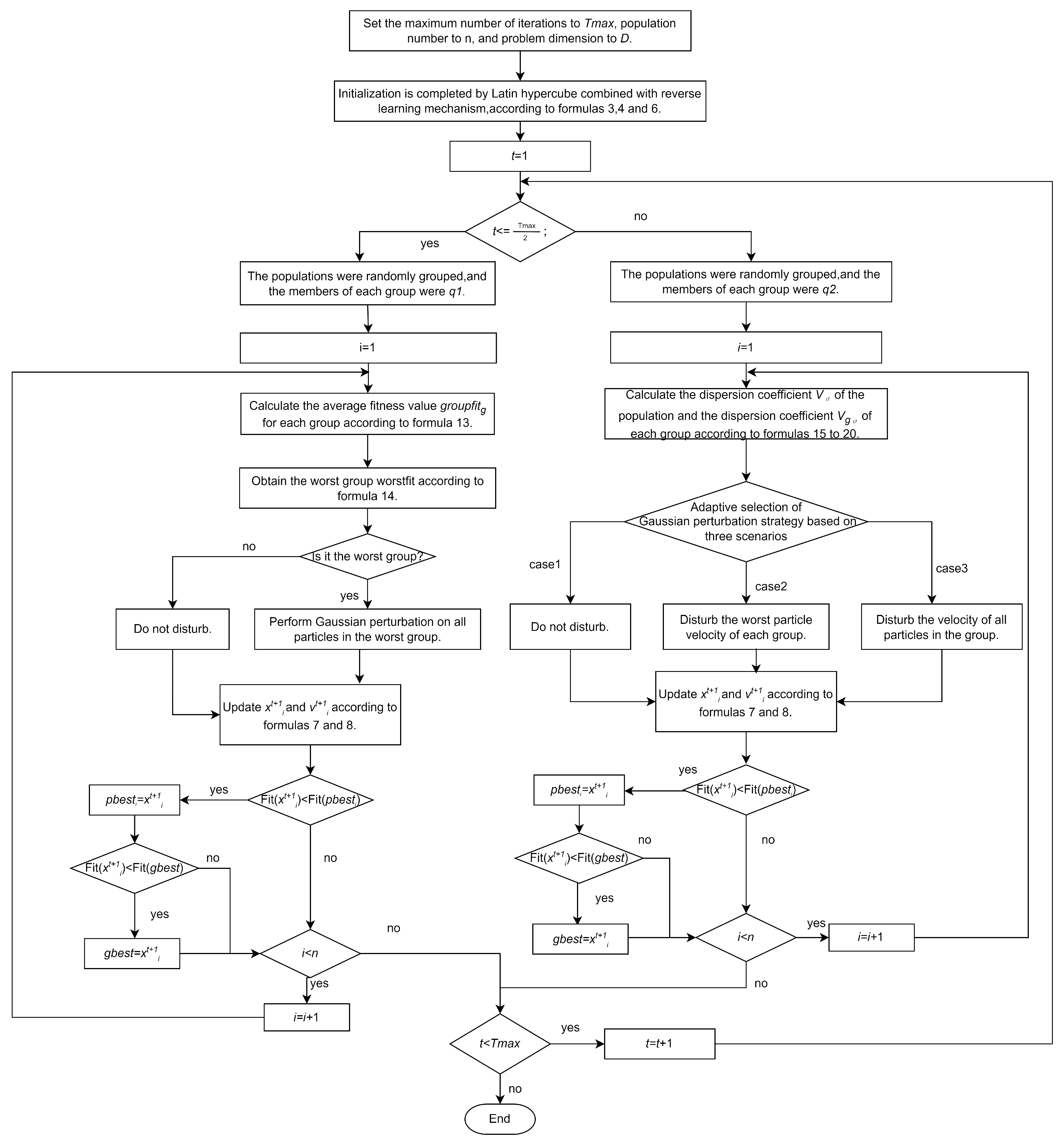
3. Group Learning Particle Swarm Optimization Algorithm

This paper proposes an adaptive perturbation Group Learning Particle Swarm Optimization (GLPSO) algorithm. The flowchart of GLPSO is shown in Figure 3.

The innovation of GLPSO lies in the following aspects: It uses Latin hypercube sampling combined with the reverse learning mechanism to initialize the population, enhancing the quality of the initial population while also improving the robustness of the algorithm. A new golden sinusoidal disturbance coefficient combined with linearly reduced inertia weight is proposed to enhance the algorithm’s global search ability in the early iteration stage, allowing the GLPSO algorithm to converge and explore the dominant region of the solution space in the later stages. Additionally, improvements are made to the random group learning of the population and the velocity updating formula, increasing the diversity of population learning and enabling particles to search the search space more comprehensively. The algorithm introduces an adaptive Gaussian perturbation strategy, allowing the velocities of the group particles to adapt to perturbations during different periods, facilitating the particles in escaping local optima for a more effective global search.

3.1. Population Initialization

Latin hypercube sampling is stratified to ensure that the particle initialization positions are evenly distributed throughout the search space, with each subspace containing only one sample. This type of distribution enhances the representativeness of the population and improves the algorithm’s global exploration capability. GLPSO sets the population size to n. A matrix $lhsDesign$ of size n is generated using Latin hypercube sampling, with values ranging between [0,1], representing relative positions uniformly distributed across the corresponding dimensions. The values in $lhsDesign$ are then mapped to the real search space $[x_{min},x_{max}]$ using scaling (6) to obtain a set of Latin populations $x_i(i=1,2,...,n)$.

$$x_i=x_{min}+(x_{max}-x_{min})·lhsDesign$$

(6)

After obtaining the Latin population through Latin hypercube sampling, the reverse population is generated using (3) $x_i(i=1,2,...,n)$. The greedy rule is then applied to select the solution with better fitness as the position of the initial particle according to (4), resulting in the formation of the initial population.

Through Latin hypercube sampling, the particles are evenly distributed in the solution space. Subsequently, the reverse solution of the original particle solutions is generated using the reverse learning mechanism, which enhances the diversity of the population. The greedy rule is then applied to select the solution with the better fitness value as the initial solution for the population, thereby improving the quality and global distribution of the initial population. As a result, the algorithm evolves from a more favorable initial state, maintains a stable global search trend throughout the iterative process, and enhances the convergence speed of the algorithm.

3.2. Stochastic Group Learning Mechanism

The original particle swarm optimization (PSO) algorithm relies on individual and global learning strategies to update particle positions, which can lead to issues such as becoming trapped in local optima and premature convergence.

In contrast, GLPSO introduces a novel random group learning strategy that enhances interaction among particles. This approach strengthens the algorithm’s global exploration capabilities, helping to mitigate the risk of premature convergence and improving the likelihood of finding more optimal solutions.

During each iteration, the population is randomly divided into groups based on the number of group members. When the number of remaining particles is insufficient to form a complete group, the remaining particles are assigned to one group. The fitness values of the particles within each group are compared, and the best particle in each group is recorded as $groupbes{t}_i^t$. During the velocity update, particles learn from their respective local best particles.

This random group learning mechanism provides particles with more opportunities to learn from different high-quality particles, enabling them to explore new directions and thereby enhancing the algorithm’s search capability. For particles that exceed the boundaries after learning, the two-sided mirror reflection boundary processing method is applied to handle their boundary conditions [39].

The velocity update method is influenced by the golden disturbance coefficient $gc$, represented by the golden inertia coefficient $g{\omega }_t$, which indicates the effect of the particle’s velocity from the previous iteration on its update. The $gc$ calculation is given by (11).

In (7), t represents the current iteration count, $pbes{t}_i$ denotes the current particle’s individual historical best position, $gbest$ represents the current global best position, and $groupbes{t}_i^t$ signifies the local best position of the group to which the current particle belongs.

The parameters $c_1$, $c_2$, and $c_3$ are learning factors, where $c_1$ indicates the influence of individual experience on the particle’s velocity update, $c_2$ represents the influence of group experience, and $c_3$ reflects the influence of group experience on the velocity update.

$$v_i^{t+1}={\omega }_t·v_i^t+c_1·r_1·(pbes{t}_i-x_i^t)+c_2·r_2·(gbest-x_i^t)+c_3·r_3·(groupbes{t}_i^t-x_i^t)$$

(7)

$$x_i^{t+1}=v_i^{t+1}+x_i^t$$

(8)

The $r_1$, $r_2$, and $r_3$ are three random numbers in the range of [0,1], representing the extent to which individual, group, and local experiences affect the current particle’s update, respectively.

The particle update mode is illustrated in Figure 4. Assuming the population size n is 9, at the t iteration, the particles in the population are randomly divided into 3 groups. The optimal particles within each group are determined based on the fitness values of the particles. In this context, the purple particle denotes the optimal particle from the group to which the yellow particle belongs. The joint influence of $pbes{t}_i$, $gbest$, and $groupbes{t}_i^t$ determines the updated position of the particle $x_i^{t+1}$.

3.3. Particle Renewal Based on Gold Disturbance Coefficient

Inertia weight ${\omega }_t$, as an essential parameter in PSO, provides particles with the adaptability to adjust to various environments, achieving a balance between exploration and exploitation. Typically, a linear inertia weight update method is used [31]. For instance, in (9), the inertia weight decreases linearly from ${\omega }_{max}$ to ${\omega }_{min}$ as the number of iterations increases [40].

This research introduces a golden sinusoidal disturbance coefficient ($gc$) in addition to the inertia weight (${\omega }_t$) of the original PSO linear transformation. The $gc$ calculation is shown in (10). The product of $gc$ and ${\omega }_t$ (denoted as $g{\omega }_t$) is used to improve particle iteration speed in (11). By combining the golden ratio coefficient with a sine function, the control strength of the golden coefficient over particle velocity decreases nonlinearly with the number of iterations.

$${\omega }_t={\omega }_{max}-({\omega }_{max}-{\omega }_{min})·{\displaystyle \frac{t}{Tmax}}$$

(9)

$$gc=g_1+g_2·(1-sin{\displaystyle \frac{pi}{2t}})·{\tau }^{-1}$$

(10)

$$g{\omega }_t={\omega }_t·gc$$

(11)

In the early iteration stages, the $g{\omega }_t$ value is large, allowing particles to explore a broader solution space, enhancing the algorithm’s global search capability and reducing the risk of premature convergence. In later iterations, the $g{\omega }_t$ value decreases, enabling particles to perform refined searches within potential optimal solution regions.

Compared with the linearly decreasing coefficient ${\omega }_t$, the $gc$ coefficient exerts a stronger initial control over particle velocity. Influenced by the sine function, its control strength decays rapidly, allowing the particles to maintain a certain velocity for local exploitation in the later stages of iteration. This type of decay better aligns with the evolutionary patterns observed in natural systems, supporting the need for fast exploration early on and slower refinement later. The $gc$ coefficient achieves a better balance between global exploration and local exploitation at different stages of the GLPSO algorithm, thereby enhancing its overall stability.

In this algorithm, the maximum iteration count is denoted by $Tmax$, and t represents the current iteration. Parameters $g_1$ and $g_2$ control the upper and lower bounds of the $gc$ coefficient, respectively. They are designed to constrain the change in particle velocity within a reasonable range, ensuring that the velocity does not become excessively large (which could destabilize the search) or too small (which could reduce the particles’ exploratory capability). After extensive experimentation, it was found that when $g_1=0.1$, the algorithm maintains a consistent level of global exploration throughout the entire process. When $g_2=1.6$, the algorithm’s exploration ability is enhanced during the early stages and gradually reduced during iteration to improve convergence. This facilitates a better balance between exploration and exploitation, under which the GLPSO algorithm achieves optimal performance. Additionally, $\tau$ is the golden ratio coefficient, which is approximately equal to 0.618.

Taking the iteration count $Tmax=1000$ as an example, the change in $g{\omega }_t$ over the iterations are shown in Figure 5. In the early stages of the iteration, their values decrease rapidly as the iteration count increases and then gradually level off in the later stages. Compared to the traditional inertia coefficient (${\omega }_t$), $g{\omega }_t$ allows for a broader exploration of the search space in the early stages of the iteration, enabling the algorithm to quickly converge towards potential optimal solution areas. In the later stages, the value of $g{\omega }_t$ levels off more than the traditional inertia coefficient (${\omega }_t$), allowing for more thorough exploration in the vicinity of the potential optimal solution area.

3.4. Adaptive Gaussian Perturbation Strategy

According to numerous experiments, perturbing particle velocity can effectively balance global and local search capabilities, preventing the algorithm from falling into local optima. GLPSO employs an adaptive Gaussian perturbation strategy to adjust particle velocity, which significantly enhances the algorithm’s convergence speed.

We apply selective Gaussian perturbation to each dimension of a particle’s velocity, with a perturbation probability $pr$. This means that each dimension of the velocity is perturbed with probability $pr$, which helps prevent particles from diverging or missing local optimal regions. It enhances the diversity and non-determinism of the search, making it more conducive to effective exploration and algorithm evolution. Multiple experiments have shown that when $pr=0.3$, the algorithm not only maintains optimization stability but also significantly improves its ability to escape local optima.

The standard deviation $sigma$ of the Gaussian perturbation is defined, and for each selected velocity dimension, a Gaussian random value, $gaussian\_vel$, is generated with a mean of 0 and a standard deviation of $sigma$. The disturbed velocity ($vel$) is then updated as shown in (12).

$$vel=gaussian\_vel·vel$$

(12)

In different update stages of small particle groups, different particles require perturbation to escape local optima. Thus, the adaptive Gaussian perturbation strategy is divided into two stages: the early iteration stage and the later iteration stage. In the early stage, there are significant differences in the average fitness values of each particle group. Based on the average fitness values and standard deviations of the different groups, targeted perturbation strategies are applied to protect high-performing particles and perturb those with lower performance, thereby enhancing the algorithm’s optimization speed.

Phase 1: The early iteration stage refers to the period from the first particle iteration to the mid-iteration; use $q1$ to represent the number of particles in each group. The group’s average fitness $groupfi{t}_m$ is calculated according to (13), where m is the number of groups, $m=(1,2,\dots ,\lceil {\displaystyle \frac{q1}{n}}\rceil )$.

When solving for the minimum of a problem, a lower fitness value indicates a better optimization result from the algorithm. If the group’s mean value is relatively high, the overall optimization performance of the particles in that group is poor, requiring perturbation. The average fitness values of each group are compared, and the group with the highest fitness value is selected as the worst-performing group. Selective Gaussian perturbation is applied to all particles in the worst-performing group by (14). Through the first phase of updating, the particle swarm evolves toward the dominant region.

$$groupfi{t}_m={\displaystyle \frac{fi{t}^1+fi{t}^2+\dots +fi{t}^{q1}}{q1}}$$

(13)

$$worstfit=argmax\{groupfi{t}_1,groupfi{t}_2,\dots ,groupfi{t}_m\}$$

(14)

Phase 2: In the later iteration stage, particles are concentrated in the advantageous region and need to learn from more prominent particles. The number of particles in each group is set to $q2$.

In this stage, the algorithm shifts from the global exploration of the first phase to the local exploitation of promising positions. Set $q2>q1$ to enable particles to strengthen the local exploitation of high-quality positions in this period. During group learning, particles benefit from learning from more dominant particles, allowing a more thorough exploration of the surrounding area.

The average fitness and standard deviation of the population are calculated using (15) and (16), while the average fitness value $groupfi{t}_m$ and standard deviation $groupst{d}_m$ of each group are calculated according to (17) and (18), respectively. Different Gaussian perturbation strategies are selected for the particle groups based on a comparison of each group’s mean and standard deviation with those of the overall population.

$$meanfit={\displaystyle \frac{{\sum }_{i=1}^{n}fi{t}^i}{n}}$$

(15)

$$std=\sqrt{{\displaystyle \frac{1}{n}}·\sum _{i=1}^n{(fi{t}^i-meanfit)}^2}$$

(16)

$meanfit$ represents the average fitness value of the population; $std$ indicates the standard deviation of the population; n is the population size; and $fit$ denotes the fitness value of particle i.

$$groupfi{t}_m={\displaystyle \frac{fi{t}^1+fi{t}^2+\dots +fi{t}^{q2}}{q2}}$$

(17)

$$groupst{d}_m=\sqrt{{\displaystyle \frac{1}{q2}}·\sum _{i=1}^{q2}{(fi{t}^i-groupfi{t}_m)}^2}$$

(18)

$groupfit$ indicates the intra-group average value of group m, and $groupstd$ represents the standard deviation of group m. To compare the dispersion degree of each group of particles, we use the dispersion coefficient for comparison. Equations (19) and (20) calculate the dispersion degree among the population particles $\left(V_{\sigma }\right)$ and the dispersion degree among the particles in group $m\left(V_{m\sigma }\right)$, respectively.

$$V_{\sigma }={\displaystyle \frac{meanfit}{std}}$$

(19)

$$V_{m\sigma }={\displaystyle \frac{groupfi{t}_m}{groupst{d}_m}}$$

(20)

When the group’s average value is less than the population average and the group dispersion coefficient is greater than or equal to that of the population t, it suggests that the particles within the group are performing ineffectively, and the worst-performing particle in the group will be perturbed to enhance the update range of the particles.

$$\left\{\begin{array}{cc}\mathrm{case}1: V_{m\sigma }\ge V_{\sigma }\hfill & \mathrm{perturb} \mathrm{the} \mathrm{worst} \mathrm{particle}\hfill \\ \mathrm{case}2: groupfi{t}_m\le meanfit\hfill \\ \hspace{1em}\hspace{1em}\hspace{1em}\mathrm{and} V_{m\sigma }<V_{\sigma }\hfill & \mathrm{leave} \mathrm{undisturbed}\hfill \\ \mathrm{case}3: groupfi{t}_m>meanfit\hfill \\ \hspace{1em}\hspace{1em}\hspace{1em}\mathrm{and} V_{m\sigma }<V_{\sigma }\hfill & \mathrm{perturb} \mathrm{the} \mathrm{whole} \mathrm{group} \mathrm{of} \mathrm{particles}\hfill \end{array}\right.$$

(21)

If the group’s average value falls below the population average and the group’s dispersion coefficient is lower than that of the population, it indicates that the particles in the group are updating effectively, and no perturbation is required for the particles within the group.

When the average value of the group is greater than the population average and the group dispersion coefficient is less than the population dispersion coefficient, it indicates that the overall performance of the particles in that group is poor, and a full group perturbation will be applied to enhance the global search capability of the particles and escape from local optima, as shown in (21).

The overall algorithm flow is shown in Algorithm 1, where the working process of GLPSO is detailed. The input parameters include the maximum number of iterations $Tmax$, population size n, and problem dimension D. The dominant population is obtained through Latin hypercube sampling combined with the reverse learning mechanism, and the historical optimal position of each particle $pbes{t}_i$ and the global optimal position of the population $gbest$ are updated. After completing the population initialization, the particles enter the iterative update phase, where different update strategies are selected to perturb the particle velocities at different stages of iteration.

Algorithm 1 GLPSO

1: Input: Population size n, maximum number of iterations $T_{\max }$, inertia weight $\omega$, location boundary $[x_{\min },x_{\max }]$, velocity boundary $[v_{\min },v_{\max }]$, $q_1=3$, $q_2=10$, $p_r=0.3$ 2: Output: Optimal solution 3: Initialize: $x_i$ is calculated by Equations (3), (4), and (6); 4: Randomly initialize velocity vector $v_i$; 5: Initialize $gbest$ and $pbest$; 6: for $t=1$ to $T_{\max }$ do 7:     if $t\le {\displaystyle \frac{T_{\max }}{2}}$ then 8:         Specify the number $q_1$ to randomize 9:         for $i=1$ to n do 10:            $groupfi{t}_m$ is calculated by (13) 11:            Find the worst group by (14) 12:            Perform Gaussian perturbation on all particles in the worst group 13:            $v_i^{t+1}$ is calculated by (7); $x_i^{t+1}$ is calculated by (8) 14:            Check the boundaries 15:            Update $gbest$; Update $pbest$ 16:         end for 17:     else 18:         Specify the number $q_2$ to randomize 19:         for $i=1$ to n do 20:            Calculate dispersion coefficient $V_{\sigma }$ of the population and $V_{g\sigma }$ for each group according to (15)–(20) 21:            Perturb different groups using the three disturbance strategies in (21). 22:            $v_i^{t+1}$ is calculated by (7); $x_i^{t+1}$ is calculated by (8) 23:            Check the boundaries 24:            Update $gbest$; Update $pbest$ 25:         end for 26:     end if 27: end for

4. Experimental Results and Discussions

4.1. Experiment Setup

In this experiment, tests were conducted on the CEC-2017 [41] test function set to evaluate the performance of GLPSO. The CEC-2017 test function set is one of the most comprehensive test suites for assessing and comparing the performance of evolutionary algorithms. These functions, shown in

Table 1. CEC2017 functions.

	No.	Functions	${\mathit{F}}_{\mathit{i}}^{*}={\mathit{F}}_{\mathit{i}}\left({\mathit{x}}^{*}\right)$
Unimodal Functions	1	Shifted and Rotated Bent Cigar Function	100
	2	Shifted and Rotated Sum of Different Power Function *	200
	3	Shifted and Rotated Zakharo Function	300
Simple Multimodal Functions	4	Shifted and Rotated Rosenbrock’s Function	400
	5	Shifted and Rotated Rastrigin’s Function	500
	6	Shifted and Rotated Expanded Scaffer’s F6 Function	600
	7	Shifted and Rotated Lunacek Bi_Rastrigin Function	700
	8	Shifted and Rotated Non-Continuous Rastrigin’s Function	800
	9	Shifted and Rotated Levy Function	900
	10	Shifted and Rotated Schwefel’s Function	1000
Hybrid Functions	11	Hybrid Function 1 (N = 3)	1100
	12	Hybrid Function 2 (N = 3)	1200
	13	Hybrid Function 3 (N = 3)	1300
	14	Hybrid Function 4 (N = 4)	1400
	15	Hybrid Function 5 (N = 4)	1500
	16	Hybrid Function 6 (N = 4)	1600
	17	Hybrid Function 6 (N = 5)	1700
	18	Hybrid Function 6 (N = 5)	1800
	19	Hybrid Function 6 (N = 5)	1900
	20	Hybrid Function 6 (N = 6)	2000
Composition Functions	21	Composition Function 1 (N = 3)	2100
	22	Composition Function 2 (N = 3)	2200
	23	Composition Function 3 (N = 4)	2300
	24	Composition Function 4 (N = 4)	2400
	25	Composition Function 5 (N = 5)	2500
	26	Composition Function 6 (N = 5)	2600
	27	Composition Function 7 (N = 6)	2700
	28	Composition Function 8 (N = 6)	2800
	29	Composition Function 9 (N = 3)	2900
	30	Composition Function 10 (N = 3)	3000
Search Range: $[-100,100{]}^D$

, are categorized into four classes: unimodal functions (f1–f3), simple multimodal functions (f4–f10), hybrid functions (f11–f20), and composition functions (f21–f22).

In this experiment, the proposed algorithm is compared with several classical meta-heuristic algorithms, including PSO [40], GA [13], and GWO [16]. To better assess the performance of the improved algorithm, GLPSO was also compared with various meta-heuristic algorithms, the classical PSO variant CLPSO [19], and advanced PSO variants such as MPSO [30], CAPSO [42], and EAPSO [25]. Details of these algorithms are provided in

Table 2. Some well-known variants of PSO and other evolution algorithms.

Algorithm	Year	Default Parameter Settings
PSO [40]	1998	D, $T_{\max }=1000$, ${\omega }_{\max }=0.9$, ${\omega }_{\min }=0.4$, $c_1=c_2=2$.
GA [13]	1998	D, $T_{\max }=1000$.
CLPSO [19]	2006	D, $T_{\max }=1000$, ${\omega }_{\max }=0.9$, ${\omega }_{\min }=0.4$, $c_1=c_2=1.49445$, $m=7$.
GWO [16]	2014	D, $T_{\max }=1000$.
MPSO [30]	2020	D, $T_{\max }=1000$, $c\omega =4\times r\times (1-r)$, $\omega =0.9\sim 0.4$, $c_1=c_2=2$.
CAPSO [42]	2022	D, $T_{\max }=1000$, ${\omega }_{\max }=0.9$, ${\omega }_{\min }=0.4$, $c_{\max }=2.5$, $c_{\min }=0.5$, $ϵ=0.2$.
EAPSO [25]	2023	D, $T_{\max }=1000$.
GLPSO	Presented	D, $T_{\max }=1000$, ${\omega }_{\max }=0.9$, ${\omega }_{\min }=0.4$, $q1=3$, $q2=10$, $pr=0.3$.

. Through extensive comparative experiments, it was confirmed that the optimal performance of GLPSO is achieved when $q1=3,q2=10$, and $pr=0.3$.

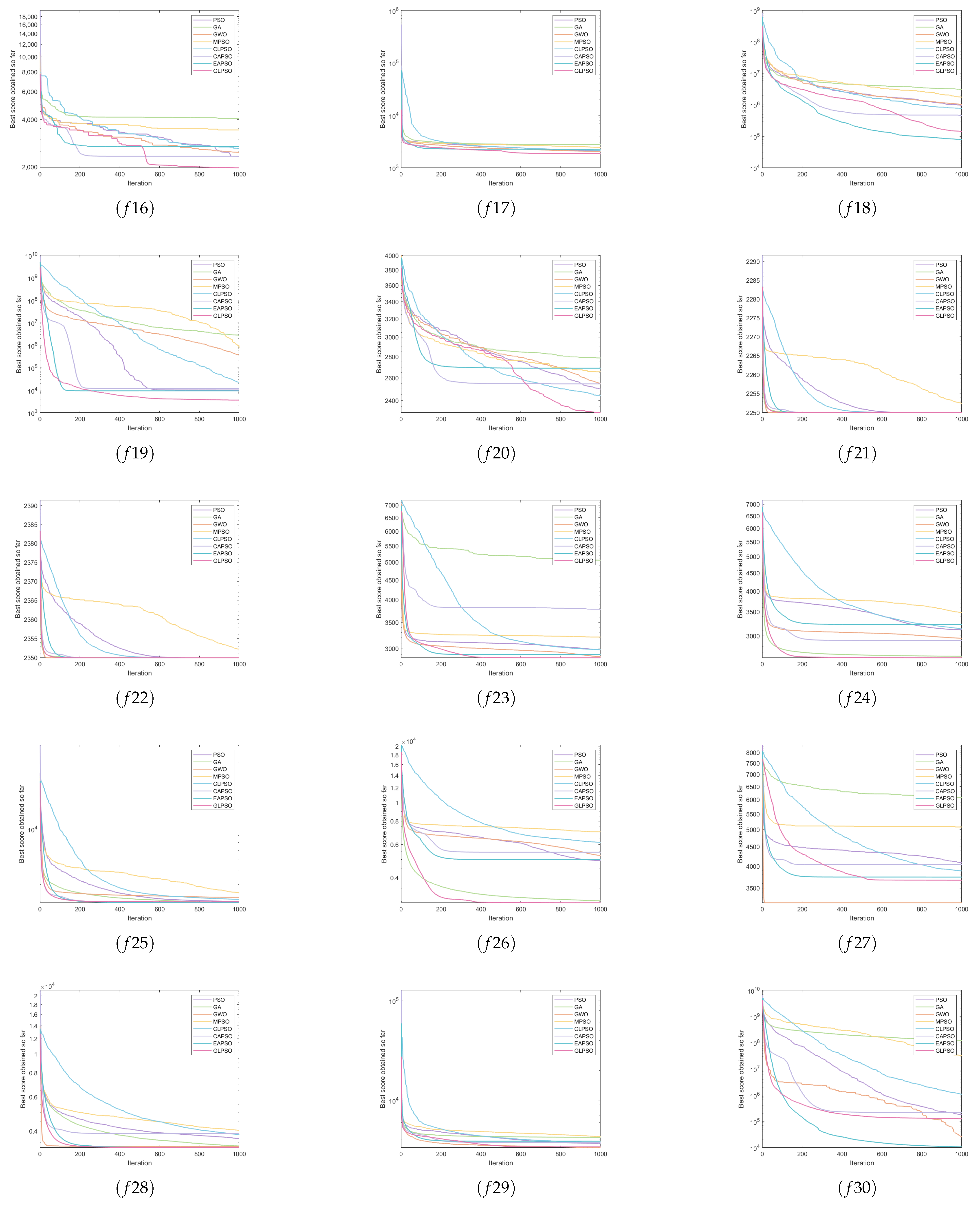
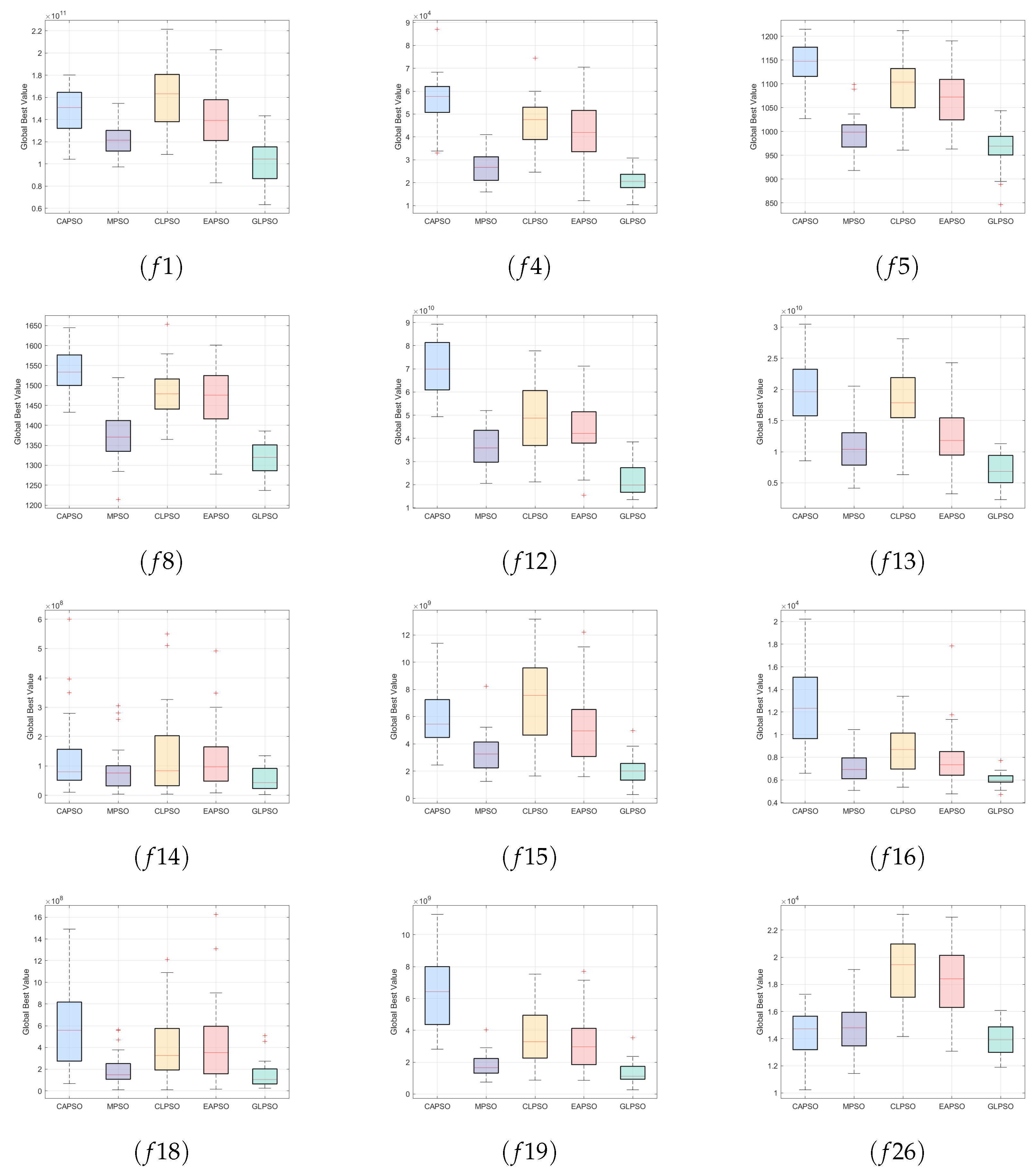
4.2. Empirical Analysis and Discussion

The proposed algorithm and the comparison algorithms were independently run 30 times on the CEC-2017 test function set in different dimensions, evaluated using three qualitative metrics. These metrics include the global optimal mean, standard deviation, and the convergence curve from 30 independent runs. A smaller mean indicates better optimization performance, while a smaller standard deviation reflects stronger robustness of the algorithm. Additionally, the algorithms’ performances are visually compared by ranking the global best mean of each algorithm. All evaluations were conducted under the same conditions, with the best results highlighted in overbold.

As shown in

Table 3. Comparisons of experimental results (30D).

		PSO	GA	GWO	MPSO	CLPSO	CAPSO	EAPSO	GLPSO
	mean	$7.95\times {10}^3$	$4.84\times {10}^{10}$	$7.83\times {10}^9$	$2.63\times {10}^9$	$3.87\times {10}^7$	$6.47\times {10}^9$	$2.00\times {10}^3$	$8.10\times {10}^4$
f1	std	$1.05\times {10}^4$	$4.36\times {10}^9$	$6.12\times {10}^9$	$1.21\times {10}^9$	$1.51\times {10}^7$	$3.83\times {10}^9$	$1.73\times {10}^3$	$1.57\times {10}^4$
	rank	2	8	7	5	4	6	1	3
	mean	$8.49\times {10}^{25}$	$4.49\times {10}^{35}$	$2.38\times {10}^{32}$	$6.66\times {10}^{31}$	$1.02\times {10}^{31}$	$3.46\times {10}^{34}$	$1.72\times {10}^{11}$	$2.68\times {10}^9$
f2	std	$3.08\times {10}^{26}$	$1.91\times {10}^{36}$	$1.24\times {10}^{33}$	$1.75\times {10}^{32}$	$2.82\times {10}^{31}$	$1.85\times {10}^{35}$	$7.15\times {10}^{11}$	$1.07\times {10}^{10}$
	rank	3	8	6	5	4	7	2	1
	mean	$5.82\times {10}^4$	$5.74\times {10}^4$	$5.24\times {10}^4$	$7.64\times {10}^4$	$1.09\times {10}^5$	$3.39\times {10}^4$	$4.56\times {10}^4$	$9.89\times {10}^3$
f3	std	$1.84\times {10}^4$	$7.75\times {10}^3$	$8.81\times {10}^3$	$1.40\times {10}^4$	$1.61\times {10}^4$	$2.09\times {10}^4$	$2.24\times {10}^4$	$4.15\times {10}^3$
	rank	6	5	4	7	8	2	3	1
	mean	$6.14\times {10}^2$	$4.53\times {10}^3$	$7.33\times {10}^2$	$1.26\times {10}^3$	$6.27\times {10}^2$	$9.88\times {10}^2$	$4.68\times {10}^2$	$5.31\times {10}^2$
f4	std	$5.20\times {10}^1$	$6.34\times {10}^2$	$1.49\times {10}^2$	$2.27\times {10}^2$	$2.54\times {10}^1$	$7.56\times {10}^2$	$4.75\times {10}^1$	$3.72\times {10}^1$
	rank	3	8	5	7	4	6	1	2
	mean	$5.93\times {10}^2$	$7.41\times {10}^2$	$6.05\times {10}^2$	$7.43\times {10}^2$	$6.52\times {10}^2$	$6.38\times {10}^2$	$6.08\times {10}^2$	$5.43\times {10}^2$
f5	std	$3.44\times {10}^1$	$3.12\times {10}^1$	$1.94\times {10}^1$	$1.64\times {10}^1$	$1.42\times {10}^1$	$3.63\times {10}^1$	$2.77\times {10}^1$	$1.05\times {10}^1$
	rank	2	7	3	8	6	5	4	1
	mean	$6.02\times {10}^2$	$6.63\times {10}^2$	$6.13\times {10}^2$	$6.59\times {10}^2$	$6.02\times {10}^2$	$6.22\times {10}^2$	$6.13\times {10}^2$	$6.00\times {10}^2$
f6	std	$1.32\times {10}^0$	$5.67\times {10}^0$	$3.60\times {10}^0$	$9.88\times {10}^0$	$4.28\times {10}^{-1}$	$1.13\times {10}^1$	$1.10\times {10}^1$	$1.29\times {10}^{-2}$
	rank	2	8	5	7	3	6	4	1
	mean	$8.40\times {10}^2$	$1.28\times {10}^3$	$9.33\times {10}^2$	$1.14\times {10}^3$	$8.89\times {10}^2$	$8.20\times {10}^2$	$8.64\times {10}^2$	$7.76\times {10}^2$
f7	std	$4.07\times {10}^1$	$5.09\times {10}^1$	$6.45\times {10}^1$	$4.69\times {10}^1$	$1.56\times {10}^1$	$2.35\times {10}^1$	$4.09\times {10}^1$	$2.89\times {10}^1$
	rank	3	8	6	7	5	2	4	1
	mean	$8.80\times {10}^2$	$1.14\times {10}^3$	$9.25\times {10}^2$	$1.03\times {10}^3$	$9.44\times {10}^2$	$9.68\times {10}^2$	$8.96\times {10}^2$	$8.54\times {10}^2$
f8	std	$3.09\times {10}^1$	$3.51\times {10}^1$	$2.94\times {10}^1$	$1.61\times {10}^1$	$1.21\times {10}^1$	$4.00\times {10}^1$	$2.25\times {10}^1$	$3.48\times {10}^1$
	rank	2	8	4	7	5	6	3	1
	mean	$1.60\times {10}^3$	$8.04\times {10}^3$	$3.82\times {10}^3$	$2.75\times {10}^3$	$3.75\times {10}^3$	$7.27\times {10}^3$	$3.14\times {10}^3$	$9.20\times {10}^2$
f9	std	$6.32\times {10}^2$	$1.35\times {10}^3$	$1.24\times {10}^3$	$4.47\times {10}^2$	$1.28\times {10}^3$	$4.26\times {10}^3$	$2.04\times {10}^3$	$2.04\times {10}^1$
	rank	2	8	6	3	5	7	4	1
	mean	$5.53\times {10}^3$	$7.32\times {10}^3$	$4.73\times {10}^3$	$8.18\times {10}^3$	$5.76\times {10}^3$	$4.84\times {10}^3$	$4.64\times {10}^3$	$4.58\times {10}^3$
f10	std	$1.54\times {10}^3$	$6.44\times {10}^2$	$1.39\times {10}^3$	$3.35\times {10}^2$	$3.59\times {10}^2$	$5.91\times {10}^2$	$7.76\times {10}^2$	$1.87\times {10}^3$
	rank	5	7	3	8	6	4	2	1
	mean	$1.24\times {10}^3$	$7.27\times {10}^3$	$4.50\times {10}^3$	$1.93\times {10}^3$	$3.63\times {10}^3$	$3.03\times {10}^3$	$1.28\times {10}^3$	$1.16\times {10}^3$
f11	std	$6.08\times {10}^1$	$1.43\times {10}^3$	$2.58\times {10}^3$	$2.20\times {10}^2$	$7.13\times {10}^2$	$8.09\times {10}^3$	$9.01\times {10}^1$	$2.68\times {10}^1$
	rank	2	8	7	4	6	5	3	1
	mean	$4.50\times {10}^6$	$6.68\times {10}^9$	$1.66\times {10}^8$	$3.54\times {10}^8$	$6.02\times {10}^7$	$6.26\times {10}^8$	$5.90\times {10}^3$	$5.69\times {10}^5$
f12	std	$6.44\times {10}^6$	$1.66\times {10}^9$	$3.77\times {10}^7$	$1.74\times {10}^8$	$2.24\times {10}^7$	$1.35\times {10}^9$	$3.14\times {10}^3$	$1.15\times {10}^5$
	rank	3	8	5	6	4	7	1	2
	mean	$3.54\times {10}^3$	$8.34\times {10}^8$	$1.87\times {10}^7$	$2.37\times {10}^7$	$4.76\times {10}^4$	$1.36\times {10}^4$	$4.64\times {10}^3$	$1.07\times {10}^4$
f13	std	$2.21\times {10}^3$	$3.21\times {10}^8$	$2.84\times {10}^7$	$2.28\times {10}^7$	$3.02\times {10}^4$	$1.59\times {10}^4$	$2.61\times {10}^3$	$2.57\times {10}^3$
	rank	1	8	6	7	5	4	2	3
	mean	$1.69\times {10}^4$	$4.81\times {10}^5$	$4.64\times {10}^5$	$1.39\times {10}^5$	$7.25\times {10}^4$	$2.42\times {10}^5$	$1.62\times {10}^3$	$1.98\times {10}^3$
f14	std	$2.35\times {10}^4$	$2.92\times {10}^5$	$9.12\times {10}^5$	$1.48\times {10}^5$	$6.30\times {10}^4$	$5.19\times {10}^5$	$1.36\times {10}^2$	$3.99\times {10}^2$
	rank	3	8	7	5	4	6	1	2
	mean	$5.32\times {10}^3$	$5.93\times {10}^7$	$1.68\times {10}^6$	$1.77\times {10}^6$	$1.82\times {10}^4$	$5.15\times {10}^3$	$1.80\times {10}^3$	$5.24\times {10}^3$
f15	std	$4.56\times {10}^3$	$2.75\times {10}^7$	$7.90\times {10}^6$	$2.17\times {10}^6$	$1.40\times {10}^4$	$5.81\times {10}^3$	$1.82\times {10}^2$	$2.63\times {10}^3$
	rank	4	8	6	7	5	2	1	3
	mean	$2.50\times {10}^3$	$4.02\times {10}^3$	$2.50\times {10}^3$	$3.37\times {10}^3$	$2.49\times {10}^3$	$2.71\times {10}^3$	$2.54\times {10}^3$	$2.14\times {10}^3$
f16	std	$3.58\times {10}^2$	$4.74\times {10}^2$	$2.85\times {10}^2$	$1.87\times {10}^2$	$1.49\times {10}^2$	$3.34\times {10}^2$	$3.83\times {10}^2$	$2.93\times {10}^2$
	rank	4	8	3	7	2	6	5	1
	mean	$2.13\times {10}^3$	$2.83\times {10}^3$	$2.05\times {10}^3$	$2.52\times {10}^3$	$2.09\times {10}^3$	$2.20\times {10}^3$	$2.25\times {10}^3$	$1.85\times {10}^3$
f17	std	$2.26\times {10}^2$	$2.04\times {10}^2$	$1.29\times {10}^2$	$2.07\times {10}^2$	$9.49\times {10}^1$	$1.98\times {10}^2$	$2.65\times {10}^2$	$6.74\times {10}^1$
	rank	4	8	2	7	3	5	6	1
	mean	$1.16\times {10}^6$	$3.34\times {10}^6$	$2.04\times {10}^6$	$1.92\times {10}^6$	$6.90\times {10}^5$	$3.10\times {10}^5$	$1.09\times {10}^5$	$1.13\times {10}^5$
f18	std	$1.27\times {10}^6$	$1.57\times {10}^6$	$2.09\times {10}^6$	$1.09\times {10}^6$	$3.70\times {10}^5$	$5.61\times {10}^5$	$1.36\times {10}^5$	$1.16\times {10}^5$
	rank	5	8	7	6	4	3	1	2
	mean	$1.22\times {10}^4$	$3.68\times {10}^6$	$1.44\times {10}^6$	$7.45\times {10}^5$	$3.21\times {10}^4$	$5.15\times {10}^5$	$1.05\times {10}^4$	$4.09\times {10}^3$
f19	std	$6.58\times {10}^3$	$3.60\times {10}^6$	$3.02\times {10}^6$	$2.47\times {10}^6$	$2.90\times {10}^4$	$1.85\times {10}^6$	$8.69\times {10}^3$	$1.97\times {10}^3$
	rank	3	8	7	6	4	5	2	1
	mean	$2.48\times {10}^3$	$2.81\times {10}^3$	$2.43\times {10}^3$	$2.62\times {10}^3$	$2.44\times {10}^3$	$2.59\times {10}^3$	$2.63\times {10}^3$	$2.32\times {10}^3$
f20	std	$2.01\times {10}^2$	$1.56\times {10}^2$	$1.50\times {10}^2$	$1.45\times {10}^2$	$1.00\times {10}^2$	$1.79\times {10}^2$	$2.22\times {10}^2$	$1.45\times {10}^2$
	rank	4	8	2	6	3	5	7	1
	mean	$2.21\times {10}^3$	$2.24\times {10}^3$	$2.20\times {10}^3$	$2.25\times {10}^3$	$2.24\times {10}^3$	$2.22\times {10}^3$	$2.20\times {10}^3$	$2.21\times {10}^3$
f21	std	$2.45\times {10}^0$	$9.12\times {10}^{-1}$	$3.97\times {10}^0$	$7.99\times {10}^{-1}$	$6.08\times {10}^{-1}$	$4.84\times {10}^0$	$2.96\times {10}^{-5}$	$8.80\times {10}^{-1}$
	rank	3	7	2	8	6	5	1	4
	mean	$2.31\times {10}^3$	$2.34\times {10}^3$	$2.30\times {10}^3$	$2.35\times {10}^3$	$2.34\times {10}^3$	$2.32\times {10}^3$	$2.30\times {10}^3$	$2.31\times {10}^3$
f22	std	$2.70\times {10}^0$	$8.31\times {10}^{-1}$	$4.16\times {10}^0$	$7.02\times {10}^{-1}$	$6.69\times {10}^{-1}$	$8.28\times {10}^0$	$1.50\times {10}^{-4}$	$5.43\times {10}^{-1}$
	rank	3	7	2	8	6	5	1	4
	mean	$2.94\times {10}^3$	$5.01\times {10}^3$	$2.87\times {10}^3$	$3.20\times {10}^3$	$2.98\times {10}^3$	$3.73\times {10}^3$	$2.88\times {10}^3$	$2.85\times {10}^3$
f23	std	$6.16\times {10}^1$	$2.53\times {10}^2$	$1.10\times {10}^2$	$3.41\times {10}^1$	$2.03\times {10}^1$	$5.42\times {10}^2$	$2.43\times {10}^1$	$2.27\times {10}^1$
	rank	6	8	3	7	5	4	1	2
	mean	$2.96\times {10}^3$	$2.72\times {10}^3$	$2.98\times {10}^3$	$2.74\times {10}^3$	$2.88\times {10}^3$	$2.74\times {10}^3$	$3.17\times {10}^3$	$2.60\times {10}^3$
f24	std	$1.81\times {10}^2$	$3.75\times {10}^2$	$2.33\times {10}^2$	$3.29\times {10}^2$	$2.48\times {10}^2$	$2.59\times {10}^2$	$2.16\times {10}^2$	$1.61\times {10}^2$
	rank	4	8	6	7	5	3	1	2
	mean	$2.99\times {10}^3$	$2.93\times {10}^3$	$3.25\times {10}^3$	$3.55\times {10}^3$	$3.14\times {10}^3$	$3.04\times {10}^3$	$2.98\times {10}^3$	$3.00\times {10}^3$
f25	std	$5.72\times {10}^1$	$2.85\times {10}^1$	$1.31\times {10}^2$	$1.46\times {10}^2$	$3.52\times {10}^1$	$2.13\times {10}^2$	$6.40\times {10}^1$	$3.78\times {10}^1$
	rank	3	1	7	8	6	5	2	4
	mean	$4.82\times {10}^3$	$3.03\times {10}^3$	$4.68\times {10}^3$	$6.95\times {10}^3$	$5.96\times {10}^3$	$5.52\times {10}^3$	$5.27\times {10}^3$	$2.91\times {10}^3$
f26	std	$1.07\times {10}^3$	$3.62\times {10}^1$	$5.27\times {10}^2$	$2.52\times {10}^2$	$5.64\times {10}^2$	$1.37\times {10}^3$	$9.53\times {10}^2$	$5.02\times {10}^2$
	rank	4	2	3	8	7	6	5	1
	mean	$4.11\times {10}^3$	$6.11\times {10}^3$	$3.20\times {10}^3$	$5.06\times {10}^3$	$3.88\times {10}^3$	$3.97\times {10}^3$	$3.72\times {10}^3$	$3.67\times {10}^3$
f27	std	$1.86\times {10}^2$	$2.44\times {10}^2$	$2.82\times {10}^{-4}$	$4.21\times {10}^2$	$8.57\times {10}^1$	$1.62\times {10}^2$	$1.36\times {10}^2$	$1.01\times {10}^2$
	rank	6	8	1	7	4	5	3	2
	mean	$3.70\times {10}^3$	$3.40\times {10}^3$	$3.31\times {10}^3$	$3.93\times {10}^3$	$3.76\times {10}^3$	$3.83\times {10}^3$	$3.33\times {10}^3$	$3.28\times {10}^3$
f28	std	$8.52\times {10}^2$	$6.63\times {10}^1$	$8.67\times {10}^1$	$7.82\times {10}^2$	$1.53\times {10}^2$	$7.38\times {10}^2$	$3.49\times {10}^2$	$2.04\times {10}^1$
	rank	5	4	2	8	6	7	3	1
	mean	$3.69\times {10}^3$	$4.15\times {10}^3$	$3.38\times {10}^3$	$4.29\times {10}^3$	$3.76\times {10}^3$	$3.77\times {10}^3$	$3.88\times {10}^3$	$3.42\times {10}^3$
f29	std	$2.03\times {10}^2$	$1.81\times {10}^2$	$2.31\times {10}^2$	$3.16\times {10}^2$	$1.41\times {10}^2$	$2.14\times {10}^2$	$2.38\times {10}^2$	$1.35\times {10}^2$
	rank	3	7	1	8	4	5	6	2
	mean	$1.16\times {10}^5$	$1.19\times {10}^8$	$1.02\times {10}^4$	$9.86\times {10}^6$	$8.78\times {10}^5$	$1.51\times {10}^5$	$9.68\times {10}^3$	$1.09\times {10}^5$
f30	std	$9.27\times {10}^4$	$6.19\times {10}^7$	$1.09\times {10}^4$	$9.82\times {10}^6$	$3.63\times {10}^5$	$1.88\times {10}^5$	$4.12\times {10}^3$	$5.40\times {10}^4$
	rank	4	8	2	7	6	5	1	3
total rank		103	209	127	201	146	152	89	53
final rank		3	8	4	7	5	6	2	1

, when D = 30, GLPSO performs well on two unimodal functions (f2–f3), but temporarily falls into local optima on f1. On the simple multimodal functions (f4–f10), its performance is excellent. These functions have multiple local optima, and the adaptive Gaussian perturbation strategy enables GLPSO to escape local optima and conduct a global search more effectively, resulting in superior performance on these problems. For the hybrid functions (f11–f20), GLPSO shows good performance, particularly on test functions f11, f16, f17, and f20. On functions f12, f18, and f19, the optimal mean achieved by GLPSO is slightly lower than that of other comparison algorithms, ranking second. However, GLPSO performs poorly on function f13. In the composition functions (f21–f30), GLPSO performs well on f23, f24, f26, f28, and f29. However, its performance on functions f21, f22, and f25 is comparatively weaker.

Figure 6 shows the convergence performance of GLPSO and the comparison algorithms on the CEC2017 test function set when D = 30, providing a more intuitive illustration of GLPSO’s convergence speed and robustness. On most multimodal and composite functions, GLPSO demonstrates strong convergence capabilities. For certain functions (f5, f8, f10, f14, f16, f20), GLPSO achieves secondary convergence during the mid-stage of the optimization process by utilizing dynamic grouping and perturbation strategies, ultimately leading to excellent optimization results. However, on a few functions (e.g., f1), GLPSO shows a disadvantage, mainly due to the nature of these functions focusing on testing the algorithm’s local exploitation ability.

GLPSO was compared with several meta-heuristic algorithms, classical PSO variants, and advanced PSO variants. The test results indicate that the proposed algorithm ranks first in the 30-dimensional CEC-2017 test functions, demonstrating its superior optimization performance, particularly in handling problems with multiple local optima. However, there are still some optimization problems where the algorithm falls into local optima, indicating that further improvements can be made.

As shown in

Table 4. Comparisons of experimental results (50D).

		PSO	GA	GWO	MPSO	CLPSO	CAPSO	EAPSO	GLPSO
	mean	$1.11\times {10}^7$	$8.91\times {10}^{10}$	$2.62\times {10}^{10}$	$1.02\times {10}^{10}$	$2.99\times {10}^7$	$1.25\times {10}^{10}$	$8.43\times {10}^3$	$2.70\times {10}^5$
f1	std	$2.08\times {10}^7$	$5.49\times {10}^9$	$8.24\times {10}^9$	$1.85\times {10}^9$	$9.29\times {10}^6$	$7.01\times {10}^9$	$9.64\times {10}^3$	$2.88\times {10}^4$
	rank	3	8	7	5	4	6	1	2
	mean	$3.67\times {10}^{49}$	$4.75\times {10}^{68}$	$2.49\times {10}^{61}$	$6.79\times {10}^{61}$	$1.18\times {10}^{30}$	$7.77\times {10}^{63}$	$2.74\times {10}^{32}$	$4.23\times {10}^{27}$
f2	std	$1.66\times {10}^{50}$	$2.38\times {10}^{69}$	$1.20\times {10}^{62}$	$3.49\times {10}^{62}$	$3.04\times {10}^{30}$	$4.25\times {10}^{64}$	$1.35\times {10}^{33}$	$2.03\times {10}^{28}$
	rank	4	8	5	6	2	7	3	1
	mean	$1.92\times {10}^5$	$1.24\times {10}^5$	$1.45\times {10}^5$	$1.92\times {10}^5$	$9.27\times {10}^4$	$1.64\times {10}^5$	$2.12\times {10}^5$	$8.13\times {10}^4$
f3	std	$3.89\times {10}^4$	$1.02\times {10}^4$	$3.69\times {10}^4$	$3.73\times {10}^4$	$1.55\times {10}^4$	$3.72\times {10}^4$	$5.75\times {10}^4$	$1.65\times {10}^4$
	rank	7	3	4	6	2	5	8	1
	mean	$7.38\times {10}^2$	$1.73\times {10}^4$	$3.09\times {10}^3$	$2.28\times {10}^3$	$6.09\times {10}^2$	$1.38\times {10}^3$	$5.16\times {10}^2$	$5.69\times {10}^2$
f4	std	$8.97\times {10}^1$	$1.79\times {10}^3$	$1.37\times {10}^3$	$6.46\times {10}^2$	$1.80\times {10}^1$	$8.89\times {10}^2$	$3.66\times {10}^1$	$4.78\times {10}^1$
	rank	4	8	7	6	3	5	1	2
	mean	$7.30\times {10}^2$	$1.05\times {10}^3$	$7.54\times {10}^2$	$9.74\times {10}^2$	$6.47\times {10}^2$	$7.98\times {10}^2$	$7.15\times {10}^2$	$5.93\times {10}^2$
f5	std	$7.42\times {10}^1$	$4.38\times {10}^1$	$3.67\times {10}^1$	$2.13\times {10}^1$	$1.31\times {10}^1$	$5.91\times {10}^1$	$6.54\times {10}^1$	$1.90\times {10}^1$
	rank	4	8	5	7	2	6	3	1
	mean	$6.11\times {10}^2$	$6.68\times {10}^2$	$6.22\times {10}^2$	$6.71\times {10}^2$	$6.02\times {10}^2$	$6.41\times {10}^2$	$6.24\times {10}^2$	$6.00\times {10}^2$
f6	std	$3.48\times {10}^0$	$4.92\times {10}^0$	$4.31\times {10}^0$	$6.82\times {10}^0$	$3.42\times {10}^{-1}$	$1.08\times {10}^1$	$7.04\times {10}^0$	$1.94\times {10}^{-1}$
	rank	3	7	4	8	2	6	5	1
	mean	$1.10\times {10}^3$	$2.00\times {10}^3$	$1.26\times {10}^3$	$1.71\times {10}^3$	$8.85\times {10}^2$	$1.03\times {10}^3$	$1.12\times {10}^3$	$8.78\times {10}^2$
f7	std	$8.91\times {10}^1$	$1.08\times {10}^2$	$9.65\times {10}^1$	$1.17\times {10}^2$	$1.44\times {10}^1$	$9.20\times {10}^1$	$8.71\times {10}^1$	$1.01\times {10}^2$
	rank	4	8	6	7	2	3	5	1
	mean	$1.00\times {10}^3$	$1.48\times {10}^3$	$1.11\times {10}^3$	$1.26\times {10}^3$	$9.40\times {10}^2$	$1.17\times {10}^3$	$1.03\times {10}^3$	$8.93\times {10}^2$
f8	std	$7.42\times {10}^1$	$3.37\times {10}^1$	$3.81\times {10}^1$	$2.22\times {10}^1$	$1.31\times {10}^1$	$7.50\times {10}^1$	$4.91\times {10}^1$	$2.11\times {10}^1$
	rank	3	8	5	7	2	6	4	1
	mean	$5.14\times {10}^3$	$2.17\times {10}^4$	$9.69\times {10}^3$	$7.01\times {10}^3$	$3.21\times {10}^3$	$2.16\times {10}^4$	$7.91\times {10}^3$	$1.04\times {10}^3$
f9	std	$3.77\times {10}^3$	$2.76\times {10}^3$	$3.35\times {10}^3$	$1.34\times {10}^3$	$5.11\times {10}^2$	$8.16\times {10}^3$	$3.32\times {10}^3$	$8.50\times {10}^1$
	rank	3	8	6	4	2	7	5	1
	mean	$1.21\times {10}^4$	$1.31\times {10}^4$	$9.07\times {10}^3$	$1.48\times {10}^4$	$5.60\times {10}^3$	$7.18\times {10}^3$	$7.49\times {10}^3$	$8.62\times {10}^3$
f10	std	$2.60\times {10}^3$	$9.59\times {10}^2$	$2.87\times {10}^3$	$5.25\times {10}^2$	$3.41\times {10}^2$	$6.72\times {10}^2$	$8.65\times {10}^2$	$3.64\times {10}^3$
	rank	6	7	5	8	1	2	3	4
	mean	$2.11\times {10}^3$	$3.31\times {10}^4$	$1.68\times {10}^4$	$7.03\times {10}^3$	$3.13\times {10}^3$	$1.25\times {10}^4$	$1.45\times {10}^3$	$1.32\times {10}^3$
f11	std	$2.36\times {10}^2$	$5.07\times {10}^3$	$8.94\times {10}^3$	$1.20\times {10}^3$	$7.50\times {10}^2$	$1.19\times {10}^4$	$1.29\times {10}^2$	$6.75\times {10}^1$
	rank	3	8	7	5	4	6	2	1
	mean	$5.63\times {10}^6$	$1.61\times {10}^{10}$	$2.84\times {10}^9$	$1.45\times {10}^9$	$5.04\times {10}^7$	$1.88\times {10}^9$	$1.23\times {10}^4$	$7.23\times {10}^5$
f12	std	$1.45\times {10}^7$	$2.85\times {10}^9$	$2.77\times {10}^9$	$6.11\times {10}^8$	$1.77\times {10}^7$	$3.83\times {10}^9$	$8.50\times {10}^3$	$3.15\times {10}^5$
	rank	3	8	7	5	4	6	1	2
	mean	$2.03\times {10}^5$	$5.65\times {10}^9$	$3.23\times {10}^8$	$3.49\times {10}^8$	$2.45\times {10}^4$	$6.20\times {10}^8$	$5.05\times {10}^4$	$5.31\times {10}^4$
f13	std	$7.92\times {10}^5$	$1.10\times {10}^9$	$3.25\times {10}^8$	$3.03\times {10}^8$	$1.30\times {10}^4$	$1.43\times {10}^9$	$5.11\times {10}^4$	$1.50\times {10}^4$
	rank	4	8	5	6	1	7	2	3
	mean	$1.72\times {10}^3$	$2.27\times {10}^6$	$1.26\times {10}^6$	$1.55\times {10}^6$	$3.17\times {10}^4$	$1.06\times {10}^6$	$1.68\times {10}^3$	$2.90\times {10}^3$
f14	std	$1.60\times {10}^2$	$1.05\times {10}^6$	$1.09\times {10}^6$	$2.11\times {10}^6$	$2.41\times {10}^4$	$3.23\times {10}^6$	$8.57\times {10}^1$	$7.51\times {10}^2$
	rank	2	8	6	7	4	5	1	3
	mean	$2.88\times {10}^3$	$1.64\times {10}^9$	$7.08\times {10}^7$	$3.53\times {10}^7$	$7.75\times {10}^3$	$1.80\times {10}^4$	$3.83\times {10}^3$	$1.26\times {10}^4$
f15	std	$1.32\times {10}^3$	$4.09\times {10}^8$	$7.79\times {10}^7$	$3.09\times {10}^7$	$5.04\times {10}^3$	$1.65\times {10}^4$	$2.24\times {10}^3$	$4.09\times {10}^3$
	rank	1	8	7	6	3	5	2	4
	mean	$3.46\times {10}^3$	$5.88\times {10}^3$	$3.54\times {10}^3$	$5.59\times {10}^3$	$2.40\times {10}^3$	$3.42\times {10}^3$	$3.27\times {10}^3$	$2.94\times {10}^3$
f16	std	$7.76\times {10}^2$	$5.49\times {10}^2$	$3.95\times {10}^2$	$3.92\times {10}^2$	$2.00\times {10}^2$	$3.80\times {10}^2$	$5.09\times {10}^2$	$6.77\times {10}^2$
	rank	5	8	6	7	1	4	3	2
	mean	$2.88\times {10}^3$	$4.07\times {10}^3$	$2.59\times {10}^3$	$3.92\times {10}^3$	$2.07\times {10}^3$	$3.03\times {10}^3$	$2.92\times {10}^3$	$2.26\times {10}^3$
f17	std	$3.35\times {10}^2$	$3.96\times {10}^2$	$3.05\times {10}^2$	$3.22\times {10}^2$	$8.74\times {10}^1$	$3.69\times {10}^2$	$3.43\times {10}^2$	$1.97\times {10}^2$
	rank	4	8	3	7	1	6	5	2
	mean	$4.55\times {10}^6$	$2.32\times {10}^7$	$4.99\times {10}^6$	$8.54\times {10}^6$	$6.64\times {10}^5$	$2.44\times {10}^6$	$7.80\times {10}^5$	$6.61\times {10}^5$
f18	std	$2.00\times {10}^6$	$8.33\times {10}^6$	$5.60\times {10}^6$	$4.86\times {10}^6$	$4.30\times {10}^5$	$1.75\times {10}^6$	$4.93\times {10}^5$	$3.28\times {10}^5$
	rank	5	8	6	7	2	4	3	1
	mean	$6.51\times {10}^5$	$1.64\times {10}^9$	$2.54\times {10}^7$	$1.81\times {10}^7$	$1.71\times {10}^4$	$8.62\times {10}^7$	$1.15\times {10}^4$	$8.83\times {10}^3$
f19	std	$2.45\times {10}^6$	$5.96\times {10}^8$	$6.05\times {10}^7$	$1.56\times {10}^7$	$1.03\times {10}^4$	$2.31\times {10}^8$	$1.17\times {10}^4$	$3.88\times {10}^3$
	rank	4	8	6	5	3	7	2	1
	mean	$3.54\times {10}^3$	$3.65\times {10}^3$	$3.13\times {10}^3$	$3.76\times {10}^3$	$2.41\times {10}^3$	$3.16\times {10}^3$	$3.19\times {10}^3$	$2.87\times {10}^3$
f20	std	$3.64\times {10}^2$	$2.31\times {10}^2$	$5.41\times {10}^2$	$1.62\times {10}^2$	$8.75\times {10}^1$	$3.50\times {10}^2$	$3.52\times {10}^2$	$5.01\times {10}^2$
	rank	6	7	3	8	1	4	5	2
	mean	$2.25\times {10}^3$	$2.25\times {10}^3$	$2.25\times {10}^3$	$2.26\times {10}^3$	$2.30\times {10}^3$	$2.25\times {10}^3$	$2.25\times {10}^3$	$2.25\times {10}^3$
f21	std	$8.39\times {10}^{-3}$	$5.40\times {10}^{-3}$	$8.53\times {10}^{-13}$	$1.35\times {10}^0$	$7.07\times {10}^1$	$5.07\times {10}^{-3}$	$8.58\times {10}^{-6}$	$3.86\times {10}^{-5}$
	rank	4	6	1	7	8	5	2	3
	mean	$2.35\times {10}^3$	$2.35\times {10}^3$	$2.35\times {10}^3$	$2.36\times {10}^3$	$3.19\times {10}^3$	$2.35\times {10}^3$	$2.35\times {10}^3$	$2.35\times {10}^3$
f22	std	$1.96\times {10}^{-3}$	$5.66\times {10}^{-3}$	$1.41\times {10}^{-12}$	$1.24\times {10}^0$	$1.22\times {10}^3$	$4.64\times {10}^{-3}$	$1.16\times {10}^{-7}$	$8.03\times {10}^{-6}$
	rank	4	6	1	7	8	5	2	3
	mean	$3.42\times {10}^3$	$7.97\times {10}^3$	$3.15\times {10}^3$	$3.94\times {10}^3$	$2.97\times {10}^3$	$5.10\times {10}^3$	$3.28\times {10}^3$	$3.08\times {10}^3$
f23	std	$1.13\times {10}^2$	$3.84\times {10}^2$	$1.21\times {10}^2$	$7.49\times {10}^1$	$1.92\times {10}^1$	$5.49\times {10}^2$	$1.02\times {10}^2$	$4.20\times {10}^1$
	rank	5	8	3	6	1	7	4	2
	mean	$3.73\times {10}^3$	$2.69\times {10}^3$	$3.53\times {10}^3$	$4.39\times {10}^3$	$3.09\times {10}^3$	$3.41\times {10}^3$	$3.72\times {10}^3$	$2.61\times {10}^3$
f24	std	$1.75\times {10}^2$	$9.08\times {10}^0$	$5.04\times {10}^2$	$1.33\times {10}^2$	$2.04\times {10}^2$	$7.71\times {10}^2$	$4.00\times {10}^2$	$6.95\times {10}^{-1}$
	rank	7	2	5	8	3	4	6	1
	mean	$3.18\times {10}^3$	$3.81\times {10}^3$	$3.96\times {10}^3$	$4.35\times {10}^3$	$3.11\times {10}^3$	$3.18\times {10}^3$	$3.06\times {10}^3$	$3.07\times {10}^3$
f25	std	$5.20\times {10}^1$	$1.56\times {10}^2$	$4.62\times {10}^2$	$3.13\times {10}^2$	$1.56\times {10}^1$	$1.63\times {10}^2$	$4.73\times {10}^1$	$3.65\times {10}^1$
	rank	5	6	7	8	3	4	1	2
	mean	$7.61\times {10}^3$	$3.31\times {10}^3$	$5.74\times {10}^3$	$1.10\times {10}^4$	$5.99\times {10}^3$	$6.60\times {10}^3$	$7.10\times {10}^3$	$2.83\times {10}^3$
f26	std	$1.20\times {10}^3$	$7.14\times {10}^1$	$2.76\times {10}^3$	$3.21\times {10}^2$	$2.58\times {10}^2$	$2.82\times {10}^3$	$2.52\times {10}^3$	$2.18\times {10}^0$
	rank	7	2	3	8	4	5	6	1
	mean	$5.33\times {10}^3$	$1.09\times {10}^4$	$3.20\times {10}^3$	$7.78\times {10}^3$	$3.82\times {10}^3$	$4.79\times {10}^3$	$4.39\times {10}^3$	$4.45\times {10}^3$
f27	std	$4.24\times {10}^2$	$4.64\times {10}^2$	$2.25\times {10}^{-4}$	$5.01\times {10}^2$	$5.93\times {10}^1$	$4.00\times {10}^2$	$3.12\times {10}^2$	$2.59\times {10}^2$
	rank	6	8	1	7	2	5	3	4
	mean	$3.93\times {10}^3$	$4.45\times {10}^3$	$3.30\times {10}^3$	$6.34\times {10}^3$	$3.79\times {10}^3$	$4.23\times {10}^3$	$3.33\times {10}^3$	$3.43\times {10}^3$
f28	std	$3.22\times {10}^2$	$1.41\times {10}^2$	$3.48\times {10}^{-4}$	$4.15\times {10}^2$	$1.84\times {10}^2$	$9.34\times {10}^2$	$3.40\times {10}^1$	$4.78\times {10}^1$
	rank	5	7	1	8	4	6	2	3
	mean	$4.72\times {10}^3$	$6.26\times {10}^3$	$3.79\times {10}^3$	$6.66\times {10}^3$	$3.71\times {10}^3$	$4.60\times {10}^3$	$4.72\times {10}^3$	$4.05\times {10}^3$
f29	std	$3.63\times {10}^2$	$4.15\times {10}^2$	$3.95\times {10}^2$	$4.33\times {10}^2$	$1.43\times {10}^2$	$3.09\times {10}^2$	$3.80\times {10}^2$	$3.17\times {10}^2$
	rank	5	7	2	8	1	4	6	3
	mean	$1.21\times {10}^6$	$6.54\times {10}^7$	$1.68\times {10}^6$	$1.65\times {10}^8$	$7.53\times {10}^5$	$2.95\times {10}^6$	$6.00\times {10}^4$	$5.64\times {10}^5$
f30	std	$1.31\times {10}^6$	$9.11\times {10}^6$	$2.68\times {10}^6$	$8.56\times {10}^7$	$3.87\times {10}^5$	$7.71\times {10}^6$	$6.19\times {10}^4$	$1.83\times {10}^5$
	rank	4	7	5	8	3	6	1	2
total rank		130	211	139	202	83	158	97	60
final rank		4	8	5	7	2	6	3	1

, when D = 50, the performance of GLPSO decreases compared to its performance in the 30-dimensional setting. However, for the CEC-2017 function set tested, GLPSO still outperforms the other comparison algorithms.

In the unimodal functions (f1–f3), GLPSO performs well on f2 and f3, while on f1, its performance is slightly worse than that of CLPSO. For the simple multimodal functions (f4–f10), GLPSO continues to perform well, although its performance on f10 is slightly lower compared to the 30-dimensional case. In the hybrid functions (f11–f20), GLPSO’s performance decreases compared to its 30-dimensional results but remains strong overall. Notably, it shows excellent optimization on functions f11, f18, and f19, while performing poorly on f13, f14, and f15. In the composition functions (f21–f30), GLPSO performs well on f23, f24, f26, f28, and f29, with only a weak performance on f27.

Based on the optimization results on the CEC-2017 test function set, GLPSO demonstrates excellent optimization performance, showing stability and strong optimization capabilities in most optimization problems. The combination of the random grouping strategy and the adaptive Gaussian perturbation strategy enables rapid secondary convergence during the mid-iteration phase.

As shown in Figure 6, functions f5, f7, f8, f10, f14, f16, f18, and f20 exhibit significantly rapid convergence during the mid-iteration phase. For the more complex composition functions (f21–f30), setting a higher number of iterations allows the improved strategy, which combines the random grouping strategy and the adaptive Gaussian perturbation strategy, to demonstrate greater advantages. The adaptive Gaussian perturbation strategy enhances the algorithm’s global search capability while maintaining robustness, achieving a balance between global exploration and local exploitation.

The Latin hypercube method ensures that particles are evenly distributed throughout the search space during initialization, which is beneficial for exploring the search space. The combination of the Latin hypercube and reverse learning strategy is employed for initialization, allowing the GLPSO algorithm to achieve a more advantageous particle population. When D = 30, the number of iterations is set to $Tmax$ = 2, and the CEC-2017 test function is independently run 30 times. The GLPSO algorithm is compared with evolutionary algorithms such as MPSO [23], CAPSO [31], and EAPSO [20] to evaluate the globally optimal particle obtained from initialization. The global optimal results of 30 particle initializations are shown in Figure 7.

As demonstrated in Figure 7, the initialization strategy of GLPSO can achieve more advantageous particle positions more consistently across four different test functions. The combination of the Latin hypercube method and the reverse learning mechanism allows the GLPSO algorithm to obtain a stable and high-quality initialization population during the initialization phase.

5. Performance Analysis

5.1. Ablation Study Analysis

To evaluate the effectiveness of each improvement in GLPSO, an ablation study was conducted for qualitative analysis of the algorithm. Specifically, three variants were tested by removing individual components from GLPSO: the $gc$ coefficient (GLPSO-gc), the group learning mechanism (GLPSO-gl), and the adaptive Gaussian perturbation strategy (GLPSO-gp). The population size was set to $N=30$, the problem dimension to $D=20$, and each algorithm, including the full GLPSO, was run on the CEC-2022 test function set [43] for 500 iterations, with 30 independent runs. The experimental results are shown in Figure 8.

The results indicate that each strategy within GLPSO is effective. These strategies interact and complement each other, balancing global exploration and local exploitation, ultimately forming a GLPSO algorithm that is both efficient and robust.

5.2. Complexity Analysis

To evaluate the computational efficiency and scalability of GLPSO, a time complexity analysis was performed for both the standard PSO algorithm and the improved algorithm. Let N be the number of particles, D be the problem dimension, T be the maximum number of iterations, C be the cost of each function evaluation, and G be the number of groups.

For standard PSO, the initialization time consists of generating the velocity and position for each particle and calculating the fitness values, which results in a complexity of $O(ND+NC)$. In the iteration phase, the complexity for each generation includes the update of velocity and position, the computation of fitness values, and the update of the global best, with a complexity of $O(ND+NC)$. Therefore, the overall time complexity of standard PSO is $O\left(TN\right(D+C\left)\right)$.

GLPSO, which uses Latin hypercube sampling combined with opposition-based learning for initialization, has a complexity of $O(NDlo{g}_2^D+NC)$ during the initialization phase. In each iteration, the algorithm performs additional computations for the standard deviation, mean, grouping, and perturbation handling, so the time complexity in this phase is $O(ND+NC)$. Thus, the overall time complexity of GLPSO is also $O\left(TN\right(D+C\left)\right)$.

In summary, the time complexity expressions for GLPSO and standard PSO are the same, but GLPSO has a larger constant factor, making its computational complexity slightly higher than that of standard PSO.

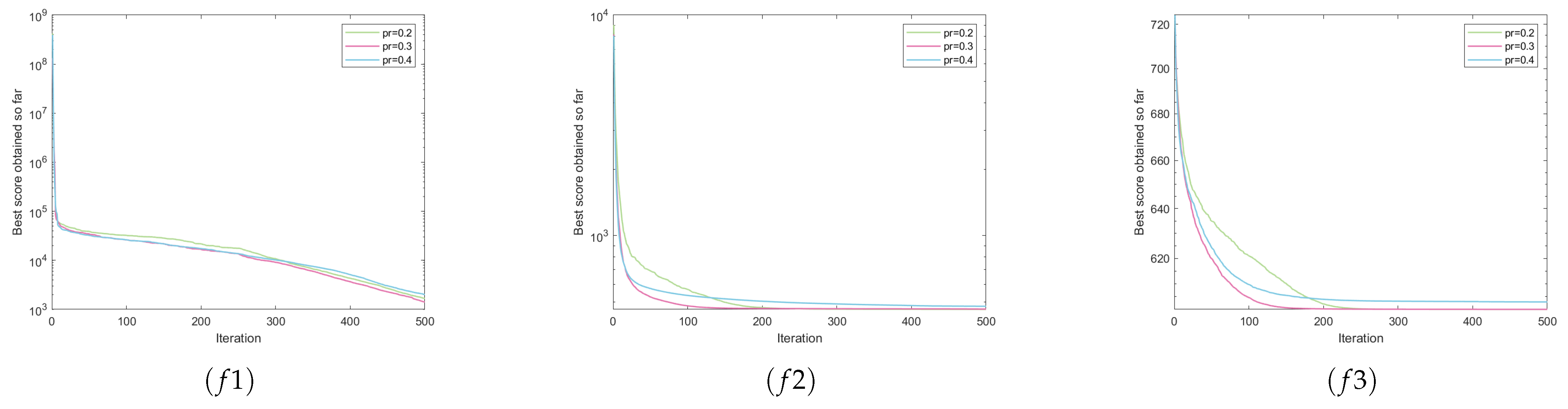
5.3. Parameter Sensitivity Analysis

To evaluate the impact of the adaptive perturbation parameter $pr$ on GLPSO, comparative experiments were conducted on the CEC-2017 and CEC2022 test function sets. Three different values of $pr$ were tested: 0.2, 0.3, and 0.4. With other parameters kept constant, 500 iterations were performed for each experiment, and each algorithm was run independently 30 times to analyze the effects of different pr values on the algorithm’s performance.

Figure 9 shows the convergence of GLPSO on the CEC2022 dataset under different perturbation rates. The experimental results indicate that when $pr$ is in the range of 0.2 to 0.4, the algorithm exhibits excellent convergence and strong robustness. On certain functions, a lower pr value leads to insufficient population diversity, causing premature convergence, while a higher pr value introduces too much randomness, affecting the convergence quality. When $pr=0.3$, GLPSO converges very quickly on certain functions (f2, f3, f5, f11).

6. Application to Engineering Problems

In previous experiments, GLPSO demonstrated excellent performance on unconstrained problems. To further evaluate its performance, the algorithm was compared with several advanced algorithms on two classic engineering problems from the 57 real-world constrained problem benchmark suite [44], with constraint handling implemented using a penalty function approach [45].

To ensure a fair comparison with other advanced algorithms, the parameter settings of GLPSO were kept consistent with those of the compared algorithms. The population size N was set to 100, and the maximum number of iterations was set to 15,000. The algorithm was independently run 30 times on the constrained problems, and the best result was recorded. The comparison results are shown in

Table 5. Optimization results of the tension/compression spring design problem.

Algorithm	The Optimal Variable			Optimal Weight
	${\mathit{x}}_{\mathbf{1}}$	${\mathit{x}}_{\mathbf{2}}$	${\mathit{x}}_{\mathbf{3}}$
PSO	0.052410681	0.374327572	10.32660253	0.012674616
PCFMO	0.052405	0.37416	10.338	0.012867
SCSO	0.0500	0.3175	14.0200	0.012717
GJO	0.0515793	0.354055	11.4484	0.01266752
BWO	0.0517	0.3568	11.3132	0.012703
DO	0.051215	0.345416	11.983708	0.012669
ICHIMP-SHO	0.051324	0.347614	11.86041	0.0126915
EAPSO	0.0515219	0.3527102	11.527838	0.012666
GLPSO	0.0514355	0.350633	11.6596	0.012671

and

Table 6. Optimization results of the weight minimization of a speed reducer.

Algorithm	The Optimal Variable							Optimal Weight
	${\mathit{x}}_{\mathbf{1}}$	${\mathit{x}}_{\mathbf{2}}$	${\mathit{x}}_{\mathbf{3}}$	${\mathit{x}}_{\mathbf{4}}$	${\mathit{x}}_{\mathbf{5}}$	${\mathit{x}}_{\mathbf{6}}$	${\mathit{x}}_{\mathbf{7}}$
GSSA	3.500957	0.70	17.00	7.331317	7.806692	3.351851	5.28669	2997.5658
ASO	3.50000	0.70	17.0755	7.3000	8.1198	3.4366	5.2935	3051.31905
HHSC	3.50379	0.70	17.00	7.3	7.7294014	3.356511	5.28669	2997.89844
AO	3.5021	0.70	17.00	7.3099	7.7476	3.3641	5.2994	3007.7328
GLPSO	3.50402	0.700099	17.012	7.37466	7.80098	3.36426	5.28804	3005.4617

. It is worth noting that the solutions for comparison were directly extracted from the corresponding reference literature.

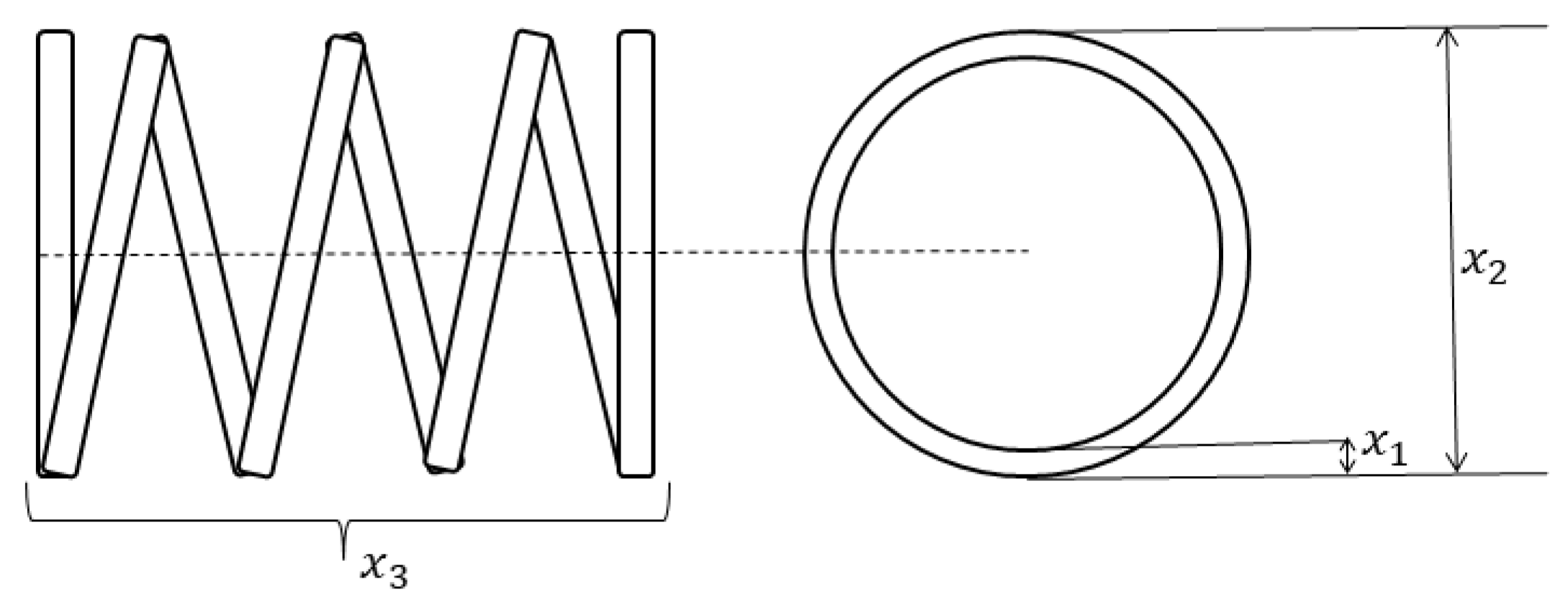
6.1. Tension/Compression Spring Design

This problem involves four constraints and three variables. As shown in Figure 10, it includes the diameter of the wire $\left(x_1\right)$, the mean diameter of the coil $\left(x_2\right)$, and the number of active coils $\left(x_3\right)$. The objective is to optimize the weight of a tension/compression spring.

The mathematical model is as follows (22):

$$\begin{array}{ccc}& \hfill \mathrm{Minimize} f\left(x\right)& =x_1^2{x}_2(2+x_3)\hfill \\ \mathrm{Subject} \mathrm{to}: \hfill & \\ & \hfill g_1\left(x\right)& =1-{\displaystyle \frac{x_2^3{x}_3}{71785x_1^4}}\le 0\hfill \\ & \hfill g_2\left(x\right)& ={\displaystyle \frac{4x_2^2-x_1{x}_2}{12566(x_2{x}_1^3-x_1^4)}}+{\displaystyle \frac{1}{5108x_1^2}}\le 0\hfill \\ & \hfill g_3\left(x\right)& =1-{\displaystyle \frac{140.45x_1}{x_2^2{x}_3}}\le 0\hfill \\ & \hfill g_4\left(x\right)& ={\displaystyle \frac{x_1+x_2}{1.5}}-1\le 0\hfill \end{array}$$

(22)

where $0.05\le x_1\le 2$, $0.25\le x_2\le 1.30$, and $2.00\le x_3\le 15$.

Table 5 presents the optimization results of GLPSO, PSO, and several advanced algorithms, including PCFMO [46], SCSO [47], GJO [48], BWO [49,50], and ICHIMP-SHO [51], on the tension/compression spring design problem. As shown in the table, GLPSO achieved an optimal objective value of 0.012671, demonstrating outstanding performance among the advanced algorithms.

6.2. Weight Minimization of a Speed Reducer

This problem involves seven variables: the face width $\left(x_1\right)$, the module of teeth $\left(x_2\right)$, the number of teeth in the pinion $\left(x_3\right)$, the length of the first shaft between bearings $\left(x_4\right)$, the length of the second shaft between bearings $\left(x_5\right)$, the diameter of the first shaft $\left(x_6\right)$, and the diameter of the second shaft $\left(x_7\right)$. The design of a small aircraft engine gearbox is optimized through seven nonlinear constraints and four linear constraints. The mathematical model is as (23):

$$\begin{array}{cc}\hfill \mathrm{Minimize} f\left(x\right)& =0.7854x_2^2{x}_1(14.9334x_3-43.0934+3.3333x_3^2)\hfill \\ \hfill & +0.7854(x_5{x}_7^2+x_4{x}_6^2)-1.508x_1(x_7^2+x_6^2)+7.477(x_7^3+x_6^3)\hfill \\ \hfill \mathrm{Subject} \mathrm{to} : \\ \hfill g_1\left(x\right)& =-x_1{x}_2^2{x}_3+27\le 0\hfill \\ \hfill g_2\left(x\right)& =-x_1{x}_2^2{x}_3^2+397.5\le 0\hfill \\ \hfill g_3\left(x\right)& =-x_2{x}_6^4{x}_3{x}_4^{-3}+1.93\le 0\hfill \\ \hfill g_4\left(x\right)& =-x_2{x}_7^4{x}_3{x}_5^{-3}+1.93\le 0\hfill \\ \hfill g_5\left(x\right)& =10x_6^{-3}\sqrt{16.91\times {10}^6+{\left(745x_4{x}_2^{-1}{x}_3^{-1}\right)}^2}-1100\le 0\hfill \\ \hfill g_6\left(x\right)& =10x_7^{-3}\sqrt{157.5\times {10}^6+{\left(745x_5{x}_2^{-1}{x}_3^{-1}\right)}^2}-850\le 0\hfill \\ \hfill g_7\left(x\right)& =x_2{x}_3-40\le 0\hfill \\ \hfill g_8\left(x\right)& =-x_1{x}_2^{-1}+5\le 0\hfill \\ \hfill g_9\left(x\right)& =x_1{x}_2^{-1}-12\le 0\hfill \\ \hfill g_{10}\left(x\right)& =1.5x_6-x_4+1.9\le 0\hfill \\ \hfill g_{11}\left(x\right)& =1.1x_7-x_5+1.9\le 0\hfill \end{array}$$

(23)

where $2.6\le x_1\le 3.6$, $0.7\le x_2\le 0.8$, $17\le x_3\le 28$, $x_4\le 8.3$,$7.3\le x_5$,$2.9\le x_6\le 3.9$, and $5\le x_7\le 5.5$.

Table 6 presents the optimization results of GLPSO, PSO, and several advanced algorithms, including GSSA [52], HHSC [53], ASO [54], and AO [55], on the weight minimization of a speed reducer problem. As shown in the table, GLPSO achieved an optimal objective value of 3005.4617, demonstrating competitive performance among the compared advanced algorithms.

The experimental data indicates that GLPSO demonstrates competitive performance among the compared algorithms, with its performance ranking at a moderate level in this engineering case. Although it outperforms some algorithms, it does not consistently surpass all other algorithms in every case. This suggests that while GLPSO excels in certain types of problems, there is still room for improvement when addressing certain types of optimization problems.

7. Conclusions

The proposed GLPSO algorithm demonstrates strong optimization capabilities on various complex benchmark functions. However, it also has some limitations stemming from its structural design. GLPSO places greater emphasis on global exploration through group learning and Gaussian perturbation mechanisms. This exploration-biased strategy may lead to slower convergence or insufficient solution accuracy when dealing with problems that require stronger local exploitation capabilities. In the future, enhancements to the algorithm’s exploitation ability will be considered to further improve its robustness and generalizability across different types of optimization problems.

References

1. Song, B.; Wang, Z.; Zou, L. On global smooth path planning for mobile robots using a novel multimodal delayed PSO algorithm. Cogn. Comput. 2017, 9, 5–17. [Google Scholar] [CrossRef]
2. Liu, Y.; Cheng, Q.; Gan, Y.; Wang, Y.; Li, Z.; Zhao, J. Multi-objective optimization of energy consumption in crude oil pipeline transportation system operation based on exergy loss analysis. Neurocomputing 2019, 332, 100–110. [Google Scholar] [CrossRef]
3. Ghorpade, S.N.; Zennaro, M.; Chaudhari, B.S.; Saeed, R.A.; Alhumyani, H.; Abdel-Khalek, S. A novel enhanced quantum PSO for optimal network configuration in heterogeneous industrial IoT. IEEE Access 2021, 9, 134022–134036. [Google Scholar] [CrossRef]
4. Bharti, V.; Biswas, B.; Shukla, K.K. A novel multiobjective gdwcn-pso algorithm and its application to medical data security. ACM Trans. Internet Technol. (TOIT) 2021, 21, 1–28. [Google Scholar] [CrossRef]
5. Awasthi, D.; Khare, P.; Srivastava, V.K. PBNHWA: NIfTI image watermarking with aid of PSO and BO in wavelet domain with its authentication for telemedicine applications. Multimed. Tools Appl. 2024, Online First. [Google Scholar] [CrossRef]
6. Lin, Y.; Jiang, Y.S.; Gong, Y.J.; Zhan, Z.H.; Zhang, J. A discrete multiobjective particle swarm optimizer for automated assembly of parallel cognitive diagnosis tests. IEEE Trans. Cybern. 2018, 49, 2792–2805. [Google Scholar] [CrossRef] [PubMed]
7. Liu, W.; Wang, Z.; Yuan, Y.; Zeng, N.; Hone, K.; Liu, X. A novel sigmoid-function-based adaptive weighted particle swarm optimizer. IEEE Trans. Cybern. 2019, 51, 1085–1093. [Google Scholar] [CrossRef]
8. Wang, Z.J.; Zhan, Z.H.; Lin, Y.; Yu, W.J.; Wang, H.; Kwong, S.; Zhang, J. Automatic niching differential evolution with contour prediction approach for multimodal optimization problems. IEEE Trans. Evol. Comput. 2019, 24, 114–128. [Google Scholar] [CrossRef]
9. Nagireddy, V.; Parwekar, P.; Mishra, T.K. Velocity adaptation based PSO for localization in wireless sensor networks. Evol. Intell. 2021, 14, 243–251. [Google Scholar] [CrossRef]
10. Shang, C.; Gao, J.; Liu, H.; Liu, F. Short-term load forecasting based on PSO-KFCM daily load curve clustering and CNN-LSTM model. IEEE Access 2021, 9, 50344–50357. [Google Scholar] [CrossRef]
11. Salihu, N.; Kumam, P.; Ibrahim, S.M.; Babando, H.A. A sufficient descent hybrid conjugate gradient method without line search consideration and application. Eng. Comput. 2024, 41, 1203–1232. [Google Scholar] [CrossRef]
12. Shen, Z.; Yang, Y.; She, Q.; Wang, C.; Ma, J.; Lin, Z. Newton design: Designing CNNs with the family of Newton’s methods. Sci. China Inf. Sci. 2023, 66, 162101. [Google Scholar] [CrossRef]
13. Mitchell, M. An Introduction to Genetic Algorithms; MIT Press: Cambridge, MA, USA, 1998. [Google Scholar]
14. Mandic, D.P. A generalized normalized gradient descent algorithm. IEEE Signal Process. Lett. 2004, 11, 115–118. [Google Scholar] [CrossRef]
15. Dorigo, M.; Birattari, M.; Stutzle, T. Ant colony optimization. IEEE Comput. Intell. Mag. 2007, 1, 28–39. [Google Scholar] [CrossRef]
16. Mirjalili, S.; Mirjalili, S.M.; Lewis, A. Grey wolf optimizer. Adv. Eng. Softw. 2014, 69, 46–61. [Google Scholar] [CrossRef]
17. Kennedy, J.; Eberhart, R. Particle swarm optimization. In Proceedings of the ICNN’95—International Conference on Neural Networks, Perth, WA, Australia, 27 November—1 December 1995; Volume 4, pp. 1942–1948. [Google Scholar] [CrossRef]
18. Li, W.; Liang, P.; Sun, B.; Sun, Y.; Huang, Y. Reinforcement learning-based particle swarm optimization with neighborhood differential mutation strategy. Swarm Evol. Comput. 2023, 78, 101274. [Google Scholar] [CrossRef]
19. Liang, J.J.; Qin, A.K.; Suganthan, P.N.; Baskar, S. Comprehensive learning particle swarm optimizer for global optimization of multimodal functions. IEEE Trans. Evol. Comput. 2006, 10, 281–295. [Google Scholar] [CrossRef]
20. Mendes, R.; Kennedy, J.; Neves, J. The fully informed particle swarm: Simpler, maybe better. IEEE Trans. Evol. Comput. 2004, 8, 204–210. [Google Scholar] [CrossRef]
21. Qu, B.Y.; Suganthan, P.N.; Das, S. A distance-based locally informed particle swarm model for multimodal optimization. IEEE Trans. Evol. Comput. 2012, 17, 387–402. [Google Scholar] [CrossRef]
22. Cao, L.; Xu, L.; Goodman, E.D. A neighbor-based learning particle swarm optimizer with short-term and long-term memory for dynamic optimization problems. Inf. Sci. 2018, 453, 463–485. [Google Scholar] [CrossRef]
23. Liu, H.R.; Cui, J.C.; Lu, Z.D.; Liu, D.Y.; Deng, Y.J. A hierarchical simple particle swarm optimization with mean dimensional information. Appl. Soft Comput. 2019, 76, 712–725. [Google Scholar] [CrossRef]
24. Huang, Y.; Li, W.; Tian, F.; Meng, X. A fitness landscape ruggedness multiobjective differential evolution algorithm with a reinforcement learning strategy. Appl. Soft Comput. 2020, 96, 106693. [Google Scholar] [CrossRef]
25. Zhang, Y. Elite archives-driven particle swarm optimization for large scale numerical optimization and its engineering applications. Swarm Evol. Comput. 2023, 76, 101212. [Google Scholar] [CrossRef]
26. Wang, F.; Zhang, H.; Zhou, A. A particle swarm optimization algorithm for mixed-variable optimization problems. Swarm Evol. Comput. 2021, 60, 100808. [Google Scholar] [CrossRef]
27. Shu, X.; Liu, Y.; Liu, J.; Yang, M.; Zhang, Q. Multi-objective particle swarm optimization with dynamic population size. J. Comput. Des. Eng. 2023, 10, 446–467. [Google Scholar] [CrossRef]
28. Zeng, N.; Zhang, H.; Chen, Y.; Chen, B.; Liu, Y. Path planning for intelligent robot based on switching local evolutionary PSO algorithm. Assem. Autom. 2016, 36, 120–126. [Google Scholar] [CrossRef]
29. Nama, S.; Saha, A.K.; Chakraborty, S.; Gandomi, A.H.; Abualigah, L. Boosting particle swarm optimization by backtracking search algorithm for optimization problems. Swarm Evol. Comput. 2023, 79, 101304. [Google Scholar] [CrossRef]
30. Das, P.K.; Jena, P.K. Multi-robot path planning using improved particle swarm optimization algorithm through novel evolutionary operators. Appl. Soft Comput. 2020, 92, 106312. [Google Scholar] [CrossRef]
31. Liu, H.; Zhang, X.W.; Tu, L.P. A modified particle swarm optimization using adaptive strategy. Expert Syst. Appl. 2020, 152, 113353. [Google Scholar] [CrossRef]
32. Li, T.; Shi, J.; Deng, W.; Hu, Z. Pyramid particle swarm optimization with novel strategies of competition and cooperation. Appl. Soft Comput. 2022, 121, 108731. [Google Scholar] [CrossRef]
33. Meng, Z.; Zhong, Y.; Mao, G.; Liang, Y. PSO-sono: A novel PSO variant for single-objective numerical optimization. Inf. Sci. 2022, 586, 176–191. [Google Scholar] [CrossRef]
34. Zhao, S.; Wang, D. Elite-ordinary synergistic particle swarm optimization. Inf. Sci. 2022, 609, 1567–1587. [Google Scholar] [CrossRef]
35. Li, G.; Li, R.; Hou, H.; Zhang, G.; Li, Z. A data-driven motor optimization method based on support vector regression—Multi-objective, multivariate, and with a limited sample size. Electronics 2024, 13, 2231. [Google Scholar] [CrossRef]
36. Wang, Y.; Zhang, J.; Zhang, M.; Wang, D.; Yang, M. Enhanced artificial ecosystem-based optimization for global optimization and constrained engineering problems. Clust. Comput. 2024, 27, 10053–10092. [Google Scholar] [CrossRef]
37. Li, C.; Zhu, Y. A hybrid butterfly and Newton–Raphson swarm intelligence algorithm based on opposition-based learning. Clust. Comput. 2024, 27, 14469–14514. [Google Scholar] [CrossRef]
38. Almansuri, M.A.K.; Yusupov, Z.; Rahebi, J.; Ghadami, R. Parameter Estimation of PV Solar Cells and Modules Using Deep Learning-Based White Shark Optimizer Algorithm. Symmetry 2025, 17, 533. [Google Scholar] [CrossRef]
39. Wang, W.X.; Li, K.S.; Tao, X.Z.; Gu, F.H. An improved MOEA/D algorithm with an adaptive evolutionary strategy. Inf. Sci. 2020, 539, 1–15. [Google Scholar] [CrossRef]
40. Shi, Y.; Eberhart, R. A modified particle swarm optimizer. In 1998 IEEE International Conference on Evolutionary Computation Proceedings; IEEE World Congress on Computational Intelligence (Cat. No. 98TH8360); IEEE: New York, NY, USA, 1998; pp. 69–73. [Google Scholar] [CrossRef]
41. Wu, G.; Mallipeddi, R.; Suganthan, P.N. Problem Definitions and Evaluation Criteria for the CEC 2017 Competition on Constrained Real-Parameter Optimization; Technical Report; National University of Defense Technology: Changsha, China; Kyungpook National University: Daegu, Republic of Korea; Nanyang Technological University: Singapore, 2017. [Google Scholar]
42. Duan, Y.; Chen, N.; Chang, L.; Ni, Y.; Kumar, S.S.; Zhang, P. CAPSO: Chaos adaptive particle swarm optimization algorithm. IEEE Access 2022, 10, 29393–29405. [Google Scholar] [CrossRef]
43. Kumar, A.; Price, K.V.; Mohamed, A.W.; Hadi, A.A.; Suganthan, P.N. Problem Definitions and Evaluation Criteria for the 2022 Special Session and Competition on Single Objective Bound Constrained Numerical Optimization; Technical Report; Nanyang Technological University: Singapore, 2021. [Google Scholar]
44. Kumar, A.; Wu, G.; Ali, M.Z.; Mallipeddi, R.; Suganthan, P.N.; Das, S. A test-suite of non-convex constrained optimization problems from the real-world and some baseline results. Swarm Evol. Comput. 2020, 56, 100693. [Google Scholar] [CrossRef]
45. Gandomi, A.H.; Yang, X.S.; Alavi, A.H. Mixed variable structural optimization using firefly algorithm. Comput. Struct. 2011, 89, 2325–2336. [Google Scholar] [CrossRef]
46. Chu, S.C.; Xu, X.W.; Yang, S.Y.; Pan, J.S. Parallel fish migration optimization with compact technology based on memory principle for wireless sensor networks. Knowl.-Based Syst. 2022, 241, 108124. [Google Scholar] [CrossRef]
47. Seyyedabbasi, A.; Kiani, F. Sand Cat swarm optimization: A nature-inspired algorithm to solve global optimization problems. Eng. Comput. 2023, 39, 2627–2651. [Google Scholar] [CrossRef]
48. Chopra, N.; Ansari, M.M. Golden jackal optimization: A novel nature-inspired optimizer for engineering applications. Expert Syst. Appl. 2022, 198, 116924. [Google Scholar] [CrossRef]
49. Zhong, C.; Li, G.; Meng, Z. Beluga whale optimization: A novel nature-inspired metaheuristic algorithm. Knowl.-Based Syst. 2022, 251, 109215. [Google Scholar] [CrossRef]
50. Zhao, S.; Zhang, T.; Ma, S.; Chen, M. Dandelion Optimizer: A nature-inspired metaheuristic algorithm for engineering applications. Eng. Appl. Artif. Intell. 2022, 114, 105075. [Google Scholar] [CrossRef]
51. Kumari, C.L.; Kamboj, V.K.; Bath, S.K.; Tripathi, S.L.; Khatri, M.; Sehgal, S. A boosted chimp optimizer for numerical and engineering design optimization challenges. Eng. Comput. 2023, 39, 2463–2514. [Google Scholar] [CrossRef]
52. Nautiyal, B.; Prakash, R.; Vimal, V.; Liang, G.; Chen, H. Improved salp swarm algorithm with mutation schemes for solving global optimization and engineering problems. Eng. Comput. 2022, 38, 3927–3949. [Google Scholar] [CrossRef]
53. Abualigah, L.; Diabat, A.; Altalhi, M.; Elaziz, M.A. Improved gradual change-based Harris Hawks optimization for real-world engineering design problems. Eng. Comput. 2023, 39, 1843–1883. [Google Scholar] [CrossRef]
54. Sun, P.; Liu, H.; Zhang, Y.; Tu, L.; Meng, Q. An intensify atom search optimization for engineering design problems. Appl. Math. Model. 2021, 89, 837–859. [Google Scholar] [CrossRef]
55. Abualigah, L.; Yousri, D.; Abd Elaziz, M.; Ewees, A.A.; Al-Qaness, M.A.; Gandomi, A.H. Aquila optimizer: A novel meta-heuristic optimization algorithm. Comput. Ind. Eng. 2021, 157, 107250. [Google Scholar] [CrossRef]
Figure 1. Particle motion illustration of PSO.
Symmetry 17 00667 g001
Figure 2. Double-sided mirror reflection diagram.
Symmetry 17 00667 g002
Figure 3. Algorithm flow chart.
Symmetry 17 00667 g003
Figure 4. Particle motion illustration of GLPSO.
Symmetry 17 00667 g004
Figure 5. The relationship between coefficient and number of iterations.
Symmetry 17 00667 g005
Figure 6. Convergence curve ( D = 30 ).
Symmetry 17 00667 g006aSymmetry 17 00667 g006b
Figure 7. Initializations of the global optimal distribution.
Symmetry 17 00667 g007aSymmetry 17 00667 g007b
Figure 8. Ablation experiment (CEC-2022).
Symmetry 17 00667 g008
Figure 9. Sensitivity analysis of the pr value (CEC-2022).
Symmetry 17 00667 g009aSymmetry 17 00667 g009b
Figure 10. Diagram of the tension and compression spring design problem.
Symmetry 17 00667 g010