Parameter Estimation of Uncertain Moving Average Model Based on Least Squares Principle

Abstract

The uncertain moving average model is a powerful tool to study the time series in which the data are affected by the previous disturbance terms under uncertain environments. However, the influence of uncertain disturbance terms is often ignored in the relevant statistical inference studies. In order to solve this problem, this paper constructs a symmetric statistical invariant, normal uncertain variable, by sorting out the uncertain moving average model and combining the uncertain disturbance terms, and then applies the least square principle to the parameter estimation of the symmetric statistical invariant to determine the unknown parameters and uncertain disturbance terms in the uncertain moving average model. In addition, a numerical algorithm is designed to calculate the corresponding estimators, and the problems related to hypothesis testing and forecast are also studied. Finally, a numerical example is given to illustrate the proposed method.

1. Introduction

Time series data are of vital importance across a wide range of essential domains, including economics, finance, environmental science, meteorology, and health care, and its importance cannot be ignored. Time series analysis is also of vital importance as a basic means to deeply analyze the intrinsic evolution of time series data and accurately predict the future trends. Looking back on the history of time series analysis, a key moment with milestone significance should date back to 1927. At that time, Yule, while carefully studying the sunspot data recorded by Wolfer, cleverly introduced the concept of autoregressive models (ARMs) in [1]. This breakthrough ushered in the era of modern time series analysis and research. Shortly thereafter, Walker [2] was inspired by the concept of autoregressive models, and conducted a comprehensive analysis of atmospheric pressure data from the Port of Darwin, India in 1931, which not only greatly broadened the application boundaries of autoregressive models and made them more widely applicable, but also innovatively proposed moving average models (MAMs) and autoregressive moving average models (ARMAMs), which combine the characteristics of ARM and MAM. These contributions have laid a firm theoretical foundation for the development of the field of time series analysis, so that it can move forward more stably. In addition, for researchers looking to gain a more profound comprehension of methods and applications of time series analysis, the works of Box and Jenkins [3] and Shumway and Stoffer [4] are indispensable resources.

It should be particularly pointed out that traditional time series analysis generally assumes that the non-deterministic phenomena inside the data originate from random fluctuations, and it usually adopts classical statistics based on probability theory to handle time series data. Nevertheless, in real-world application scenarios, the sources of non-deterministic phenomena in time series data are diverse and intricate, and there frequently occurs a situation of frequency instability. In view of this situation, numerous scholars have carried out a substantial number of empirical studies with the aim of exploring whether the non-deterministic phenomena in time series data can be reduced to randomness in real situations. For example, Yang and Liu [5] utilized partial differential equations to characterize the size of the Chinese population under different age structures, and discovered that if the non-deterministic phenomena in the population system were treated as randomness, then the resulting outcomes would conflict with the relevant assumptions. Another example is the study of Liu et al. [6], which modeled the order data of an online car-hailing platform in Beijing with the help of the theory of renewal process, and found that if the numbers of passengers were regarded as random variables, then the actual data collected would deviate from the corresponding 99% confidence interval very seriously. Therefore, if the non-deterministic phenomenon in time series data is simply reduced to randomness, it is highly likely to cause bias in the prediction of the constructed time series model and the support it provides for decision making. As a result, the accuracy and credibility of the results are also affected. For the purpose of handling this problem, and more comprehensively describing and effectively dealing with the non-deterministic phenomenon in time series data among practical applications, we are in urgent need of introducing a new axiomatic mathematical system, uncertainty theory, which was established by Liu [7] and further refined by Liu [8]. The time series analysis based on this theory is called uncertain time series analysis. Specifically, it is a collection of technical methods to collect, model and interpret time series data, evolving from uncertainty theory as a technical tool. The pioneering research work in this field commenced with the study by Yang and Liu [9], which defined the uncertain autoregressive model based on uncertainty theory.

Although some scholars have conducted corresponding studies on the least squares estimation of unknown parameters and the least squares estimation of disturbance terms in the uncertain moving average model, the previous studies completely ignored the existence of disturbance terms when estimating unknown parameters, did not comprehensively describe the influence of disturbance terms on the observed data, and separated the estimation of unknown parameters from the estimation of disturbance terms. In this paper, a symmetric statistical invariant containing unknown parameters of the uncertain moving average model is constructed by deforming the uncertain moving average model and combining the uncertainty distribution of the disturbance terms. Then, the statistical inference problem of the uncertain moving average model is transformed into the parameter estimation problem of the symmetric statistical invariant, and the corresponding estimators are determined by the least square principle. Specifically, the main contributions of this paper are as follows:

•

Based on the uncertain moving average model after deformation and the properties of uncertain disturbance terms, a symmetric statistical invariant containing unknown parameters of the uncertain moving average model is constructed.

•

The corresponding estimators are determined by combining the least squares principle, and a numerical algorithm is designed to solve the corresponding estimators.

•

A numerical example is provided to illustrate the corresponding theoretical results.

2. Literature Review of Uncertain Time Series Analysis

Since the concept of uncertain time series analysis was put forward, a large number of scholars have carried out in-depth research on it, and uncertain time series analysis has gradually developed into a relatively large-scale and mature theoretical branch within the field of uncertain statistics.

In the research of uncertain time series analysis, the primary and core content is the exploration of various uncertain time series models. The earliest uncertain time series model is the uncertain autoregressive model proposed by Yang and Liu [9]. In their research work, they made the assumption that the specific values of the time series will be influenced by both the data observed in the past and the disturbance term at the current moment. Moreover, they defined the disturbance term as an uncertain variable. This pioneering research achievement has established an important theoretical foundation for subsequent research on uncertain time series analysis. Following that, Lu et al. [10] pointed out that the future values of time series data may not only be affected by historical observed data, but may even be jointly influenced by past observed data and historical disturbance terms. In order to deal with this special phenomenon, they creatively proposed the uncertain moving average model and the uncertain autoregressive moving average model, enabling more accurate modeling and analysis of the corresponding time series data. In the meantime, Tang [11] keenly perceived the complex characteristics of multivariate time series and then proposed the uncertain vector autoregressive model. This model performs more excellently in capturing the complex relationships between variables and can more accurately reflect the actual situation. On the basic of the above results, Tang [12] then conducted related research on the time series data evolving from nonlinear relations and proposed the uncertain max autoregression model. The main purpose of this model is to effectively describe and characterize time series systems that are heavily influenced by historical extreme observations. Soon afterwards, in further research work, Tang [13] proposed the concept of the uncertain threshold autoregression model for modeling and analogizing the time series data evolving from the system with different change rules at different stages. In addition, when the system generating the time series data is completely unknown, that is, it is impossible to determine the specific form of the uncertain time series model, the research results of Zhang and Gao [14] provide us with a very powerful and effective tool for studying non-parametric time series systems. Overall, this series of rich research achievements has not only greatly enriched and improved the theoretical system framework of uncertain time series analysis, but also provided very solid and reliable technical support and a guarantee for numerous practical application scenarios.

Another important research direction of uncertain time series analysis lies in the statistical inference of uncertain time series models. This aspect plays a vital bridging role in uncertain time series analysis, closely linking theoretical methods with practical applications. To be specific, the statistical inference work for uncertain time series models mainly encompasses two vitally important core tasks. Firstly, it is necessary to accurately estimate the unknown parameters within the model, enabling the model to better fit the time series data. Secondly, it is essential to conduct a reasonable quantitative analysis of the uncertain disturbance term of the model. In terms of estimating unknown parameters, Yang and Liu [9] first proposed the least squares estimation method, whose core idea is to continuously adjust the parameters to minimize the sum of the squares of the deviations between the predicted values of the model and the actual observed values. However, considering that extreme outliers may exist in actual data and these outliers can significantly affect the results of the least squares estimation, Yang et al. [15] further proposed the least absolute deviation estimation method. This method effectively improves the accuracy of parameter estimation by minimizing the sum of the absolute values of the deviations. Beyond that, many scholars are also actively exploring other estimation methods. For example, Chen and Yang [16] successfully applied the idea of uncertain maximum likelihood to the estimation of unknown parameters in uncertain autoregressive models. Other parameter estimation methods can be found in lasso estimation (Zhang et al. [17]), ridge estimation (Chen and Yang [18]), Huber estimation (Liu [19]), moment estimation (Liu and Qin [20]), and so on. These different estimation methods all play important roles in the field of parameter estimation of uncertain time series models and demonstrate their respective values. In the field of estimating the uncertain disturbance terms, the pioneering research conducted by Yang and Liu [9] laid a solid foundation for the subsequent moment estimation method. Later, Chen and Yang [16] introduced the uncertain maximum likelihood estimation method and further promoted the development of the research of this field. However, due to the presence of outliers in actual data, which may lead to biases in the estimation results, Liu and Liu [21] studied an improved uncertain maximum likelihood estimation method. This new method has a stronger adaptability to potential data biases. In addition, Liu and Liu [22] also studied a least squares estimation method. This method estimates the uncertain disturbance terms by minimizing the sum of the deviations between the empirical distribution of the observed values and the population distribution.

3. Deformation of Uncertain Moving Average Model

In the field of uncertain time series analysis, a common assumption is that a series of observations indexed in time are available, called time series data, as follows:

$$X_t,t=1,2,\cdots ,n.$$

(1)

In order to model the time series data in the scenario where current data are more likely to be affected by previous disturbance items, Yang and Ni [23] introduced the uncertain moving average model to smooth such time series data, and then explored the long-term trend and periodic changes of time series data. Based on the assumption of a linear relationship between observations and uncertain disturbance terms, the model successfully removes short-term fluctuations and noise components in the data, and has practical applications in many fields such as market forecasting and climate change research.

Consider an uncertain moving average model of order p which is denoted as

$$X_t=a_0+{ϵ}_t-\sum _{i=1}^p{a}_i{ϵ}_{t-i}.$$

(2)

Here, ${ϵ}_t$, ${ϵ}_{t-1}$, ⋯, ${ϵ}_{t-p}$ are called the uncertain disturbance terms, and are assumed to be independent and follow the same uncertainty distribution, uncertain normal distribution $\mathcal{N}(0,\sigma )$, while $a_0$, $a_1$, ⋯, $a_p$ are a set of unknown parameters, which reflect the weights given to each uncertain disturbance term. With the help of the backshift operator B (satisfying $B^k{ϵ}_t={ϵ}_{t-k}$), the p order uncertain moving average model (2) can be reformulated as

$$X_t-a_0={ϵ}_t-\sum _{i=1}^p{a}_i{B}^i{ϵ}_t=\left(1-\sum _{i=1}^p{a}_i{B}^i\right){ϵ}_t=\Theta \left(B\right){ϵ}_t,$$

(3)

where

$$\Theta \left(B\right)=1-\sum _{i=1}^p{a}_i{B}^i.$$

In order to calculate the corresponding disturbance term based on time series data, Xin et al. [24] proved that Formula (3) is reversible, and can be written as

$${ϵ}_t={\displaystyle \frac{1}{\Theta \left(B\right)}}\left(X_t-a_0\right),$$

where

$${\displaystyle \frac{1}{\Theta \left(B\right)}}=\sum _{i=0}^{\infty }{\pi }_i{B}^i,{\pi }_0=1,{\pi }_i=\sum _{j=1}^{p\wedge i}{a}_j{\pi }_{i-j},p\wedge i=min(p,i).$$

Thus, we have

$${ϵ}_t=\sum _{i=0}^{\infty }{\pi }_i{B}^i\left(X_t-a_0\right)=\sum _{i=0}^{\infty }{\pi }_i\left(X_{t-i}-a_0\right),$$

Since the minimum index of time series data (1) starts from 1, we set $X_t=a_0$ if $t\le 0$. Then, we have

$${ϵ}_t=\sum _{i=0}^{t-1}{\pi }_i\left(X_{t-i}-a_0\right)=X_t-a_0+\sum _{i=1}^{t-1}{\pi }_i\left(X_{t-i}-a_0\right).$$

Based on the above analysis, we can rewrite the p order uncertain moving average model (2) as

$$X_t=a_0-\sum _{i=1}^{t-1}{\pi }_i\left(X_{t-i}-a_0\right)+{ϵ}_t$$

(4)

for $t=1,2,\cdots ,n$.

4. Parameter Estimation of Uncertain Moving Average Model

In this section, we will discuss the parameter estimation of uncertain moving average model based on time series data and least squares principle.

For a given set of time series data (1), it follows from the deformation expression (4) and the normality assumption of the uncertain disturbance terms that

$${ϵ}_t=X_t-a_0+\sum _{i=1}^{t-1}{\pi }_i\left(X_{t-i}-a_0\right)\sim \mathcal{N}(0,\sigma ).$$

(5)

By defining the following n real functions with unknown parameters $a_0$, $a_1$, ⋯, $a_p$ and $\sigma$ as

$$h_t(a_0,a_1,\cdots ,a_p,\sigma )={\displaystyle \frac{{\displaystyle X_t-a_0+\sum _{i=1}^{t-1}{\pi }_i\left(X_{t-i}-a_0\right)}}{\sigma }},t=1,2,\cdots ,n,$$

(6)

it is not difficult to infer that when the unknown parameters $a_0$, $a_1$, ⋯, $a_p$ and $\sigma$ in the p order uncertain moving average model (2) can take on true values, these n real functions $h_1,h_2,\cdots ,h_n$ can be regarded as n samples of the standard normal uncertainty distribution $\mathcal{N}(0,1)$. That is, we have

$$h_1,h_2,\cdots ,h_n\sim \mathcal{N}(0,1).$$

(7)

Here, Equation (6) is the statistical invariant that we want to construct, and notice that its uncertainty distribution, standard normal uncertainty distribution $\mathcal{N}(0,1)$, is symmetric about the origin, so it is also a symmetric statistical invariant.

Based on the above analysis, we know that the n real functions $h_1,h_2,\cdots ,h_n$ defined above can be regarded as a set of samples of standard normal uncertainty distribution $\mathcal{N}(0,1)$ when the unknown parameters $a_0$, $a_1$, ⋯, $a_p$ and $\sigma$ take true values. Therefore, in order to estimate the values of the unknown parameters, we should find the set of parameters that makes the empirical distribution function of $h_1,h_2,\cdots ,h_n$ most close to the uncertainty distribution of $\mathcal{N}(0,1)$. It should be noted that the empirical distribution corresponding to $h_1,h_2,\cdots ,h_n$ is given by

$$F\left(x\right)={\displaystyle \frac{1}{n}}\sum _{t=1}^n\mathbb{I}(h_t\le x).$$

Here, $\mathbb{I}(h_t\le x)$ is the indicator function which takes the value of 1 when $h_t\le x$ and takes the value of 0 when $h_t>x$. Moreover, the expression of the uncertainty distribution of $\mathcal{N}(0,1)$ is

$$\Phi \left(x\right)={\left(1+exp\left({\displaystyle \frac{-\pi x}{\sqrt{3}}}\right)\right)}^{-1}.$$

According to the idea of the least squares principle, we can choose the parameter values that minimizes the sum of squares of the deviation between the empirical distribution $F\left(x\right)$ and the uncertainty distribution $\Phi \left(x\right)$ as the estimated parameters, that is, the least squares estimation of p order uncertain moving average model (2) should solve the following minimization problem:

$$\begin{array}{cc}\hfill & \underset{a_0,a_1,\cdots ,a_p,\sigma >0}{min}\sum _{t=1}^n{\left({\left(1+exp\left({\displaystyle \frac{-\pi h_t}{\sqrt{3}}}\right)\right)}^{-1}-{\displaystyle \frac{1}{n}}\sum _{j=1}^n\mathbb{I}(h_j\le h_t)\right)}^2.\hfill \end{array}$$

(8)

It is worth noting that the core challenge in solving the above optimization problem is the nonlinear connection between the decision variables and the objective function, because the decision variables are not only contained in the normal uncertainty distribution function, but also in the indicator function. This form makes the process of directly solving the optimization problem very difficult. To address this issue, we carefully designed and effectively implemented an algorithmic approach (Algorithm 1) whose key goal is to effectively process and approximate the least squares solution of the optimization problem, thereby achieving efficient exploration and solution of the problem.

Algorithm 1 Numerical algorithms for least squares estimation

Step 0: Input time series $X_t,t=1,2,\cdots ,n$. Step 1: Determine the feasible regions $\mathcal{A}$ of unknown parameters vector $(a_0,a_1,\cdots ,a_p,\sigma )$. Step 2: For each $(a_0,a_1,\cdots ,a_p,\sigma )\in \mathcal{A}$ and $\sigma >0$, compute ${\pi }_1$, ${\pi }_2$,⋯,${\pi }_{n-1}$ by $${\pi }_i=\sum _{j=1}^{p\wedge i}{a}_j{\pi }_{i-j},i=1,2,\cdots ,n-1,$$ and $h_1$, $h_2$, ⋯, $h_n$ by $$h_t={\displaystyle \frac{{\displaystyle X_t-a_0+\sum _{i=1}^{t-1}{\pi }_i\left(X_{t-i}-a_0\right)}}{\sigma }},t=1,2,\cdots ,n.$$ Step 3: Set $t=1$ and $E\left(a_0,a_1,\cdots ,a_p,\sigma \right)=0$. Step 4: Set $$\begin{array}{c}E\left(a_0,a_1,\cdots ,a_p,\sigma \right)=E\left(a_0,a_1,\cdots ,a_p,\sigma \right)+{\left({\left(1+exp\left({\displaystyle \frac{-\pi h_t}{\sqrt{3}}}\right)\right)}^{-1}-{\displaystyle \frac{1}{n}}\sum _{j=1}^n\mathbb{I}(h_j\le h_t)\right)}^2,\hfill \end{array}$$ and $t=t+1$. Step 5: If $t\le n$, then go to Step 4. Step 6: Find ${\widehat{a}}_0,{\widehat{a}}_1,\cdots ,{\widehat{a}}_p$ and $\widehat{\sigma }$ such that $E\left(a_0,a_1,\cdots ,a_p,\sigma \right)$ reaches its minimum value. Step 7: Output ${\widehat{a}}_0,{\widehat{a}}_1,\cdots ,{\widehat{a}}_p$ and $\widehat{\sigma }$.

Remark 1.

The feasible regions $\mathcal{A}$ in the above algorithm refer to a set of all possible values of unknown parameters vector $(a_0,a_1,\cdots ,a_p,\sigma )$. In addition, the function $E\left(a_0,a_1,\cdots ,a_p,\sigma \right)$ defined above is essentially a process variable used to calculate the objective function in the optimization problem (8). In particular, when $t=n$, the obtained $E\left(a_0,a_1,\cdots ,a_p,\sigma \right)$ is just the objective function in the optimization problem (8).

5. Uncertain Hypothesis Testing and Forecasting

Based on the estimated parameters ${\widehat{a}}_0,{\widehat{a}}_1,\cdots ,{\widehat{a}}_p,\widehat{\sigma }$ using the least squares principle, we can obtain an estimated uncertain moving average model. In order to facilitate the subsequent derivation, we still use the deformed uncertain moving average model here, that is,

$$X_t={\widehat{a}}_0-\sum _{i=1}^{t-1}{\widehat{\pi }}_i\left(X_{t-i}-{\widehat{a}}_0\right)+{\widehat{ϵ}}_t,$$

(9)

where ${\widehat{ϵ}}_t$ follows the uncertain normal distribution $\mathcal{N}(0,\widehat{\sigma })$. Then, the next key question is whether the estimated uncertain moving average model (9) is reasonable, and how to predict the value of time series data at future moments based on the estimated uncertain moving average model (9).

5.1. Uncertain Hypothesis Test

Before evaluating whether the estimated uncertain moving average model (9) is reasonable, we first calculate the corresponding residual series

$${\epsilon }_t=X_t-{\widehat{a}}_0+\sum _{i=1}^{t-1}{\widehat{\pi }}_i\left(X_{t-i}-{\widehat{a}}_0\right),t=1,2,\cdots ,n,$$

which can be regarded as the samples of the uncertain disturbance terms ${\widehat{ϵ}}_t$, $t=1,2,\cdots ,n$, respectively. If the estimated uncertain moving average model (9) is reasonable, that is, it can fit the given time series data (1) well, then according to the normality assumption (5) in the uncertain moving average model (4), these n residual terms ${\epsilon }_1,{\epsilon }_2,\cdots ,{\epsilon }_n$ should be a set of samples from the population $\mathcal{N}(0,\widehat{\sigma })$. At this point, testing whether the estimated uncertain moving average model (9) is reasonable is equivalent to testing whether those obtained n residuals ${\epsilon }_1,{\epsilon }_2,\cdots ,{\epsilon }_n$ are a set of samples of $\mathcal{N}(0,\widehat{\sigma })$.

According to the uncertain hypothesis test proposed by Ye and Liu [25], for a given significance level $\alpha$, if the residuals ${\epsilon }_1,{\epsilon }_2,\cdots ,{\epsilon }_n$ are indeed a set of samples of population $\mathcal{N}(0,\widehat{\sigma })$, then there should be no more than $\alpha$ points in the residuals ${\epsilon }_1,{\epsilon }_2,\cdots ,{\epsilon }_n$ beyond the $1-\alpha$ confidence interval of population $\mathcal{N}(0,\widehat{\sigma })$, where the $\alpha$ confidence interval of population $\mathcal{N}(0,\widehat{\sigma })$ is

$$\left[{\Phi }^{-1}\left({\displaystyle \frac{\alpha }{2}}\right),{\Phi }^{-1}\left({\displaystyle 1-\frac{\alpha }{2}}\right)\right]$$

and

$${\Phi }^{-1}\left(\alpha \right)={\displaystyle \frac{\sqrt{3}\widehat{\sigma }}{\pi }}ln{\displaystyle \frac{\alpha }{1-\alpha }}$$

is the inverse uncertainty distribution of population $\mathcal{N}(0,\widehat{\sigma })$. Based on this idea, we can give the rejection region W to test whether the estimated uncertain moving average model (9) is suitable. That is,

$$\begin{array}{cc}\hfill W=\left\{\right({\epsilon }_1,{\epsilon }_2,\cdots ,{\epsilon }_n):& \mathrm{there} \mathrm{are} \mathrm{at} \mathrm{least}\lfloor n\times \alpha +1\rfloor \mathrm{of} \mathrm{indexes}{t}^{\prime }\mathrm{s} \mathrm{with} 1\le t\le n\hfill \\ \hfill & \mathrm{such} \mathrm{that} {\epsilon }_t<{\Phi }^{-1}\left({\displaystyle \frac{\alpha }{2}}\right) \mathrm{or} {\epsilon }_t>{\Phi }^{-1}\left({\displaystyle 1-\frac{\alpha }{2}}\right)\}\hfill \end{array}$$

(10)

where $\lfloor x\rfloor$ represents the maximum integer not exceeding x. When we perform the test, we can do so by determining whether the obtained residual sequence ${\epsilon }_1,{\epsilon }_2,\cdots ,{\epsilon }_n$ belongs to the rejection region W. If the residuals sequence falls within the rejection region W, i.e.,

$$({\epsilon }_1,{\epsilon }_2,\cdots ,{\epsilon }_n)\in W,$$

In this case, we can only infer that the estimated uncertain moving average model (9) does not provide an optimal fit for time series data (1) and is not reasonable. Conversely, if the residuals sequence is not in the above rejected region, i.e.,

$$({\epsilon }_1,{\epsilon }_2,\cdots ,{\epsilon }_n)\notin W,$$

then we can reasonably conclude that the estimated uncertain moving average model (9) has a good fit to the time series data (1) and is reasonable.

5.2. Forecast Value and Forecast Interval

If the uncertain hypothesis test shows that the estimated uncertain moving average model (9) is reasonable, then the next step is to forecast the time series data for the future moments.

Assume that we need to forecast the time series data at time $n+1$, then the time series data at time $t=1,2,\cdots ,n$ are all known. At this point, we can substitute the known time series data $X_t$, $t=1,2,\cdots ,n$ into the estimated uncertain moving average model (9) to obtain the forecast uncertain variable ${\widehat{X}}_{n+1}$ at time $n+1$ as

$${\widehat{X}}_{n+1}={\widehat{a}}_0-\sum _{i=1}^n{\widehat{\pi }}_i\left(X_{n+1-i}-{\widehat{a}}_0\right)+\mathcal{N}(0,\widehat{\sigma }).$$

(11)

However, the forecast information needed in practice is often certain, and the above forecast uncertain variable ${\widehat{X}}_{n+1}$ is still an uncertain variable in essence, which still contains a lot of uncertainty. Therefore, we also need to give the forecast value and forecast interval of $X_{n+1}$ based on the above forecast uncertain variable ${\widehat{X}}_{n+1}$.

Note that the forecast uncertain variable ${\widehat{X}}_{n+1}$ is a normal uncertain variable whose uncertainty distribution is

$${\displaystyle {\widehat{\Phi }}_{n+1}\left(x\right)=\frac{1}{1+exp\left({\displaystyle \frac{{\displaystyle \pi }}{\sqrt{3}\widehat{\sigma }}\left({\widehat{a}}_0-\sum _{i=1}^n{\widehat{\pi }}_i\left(X_{n+1-i}-{\widehat{a}}_0\right)-x\right)}\right)},}$$

and inverse uncertainty distribution is

$${\widehat{\Phi }}_{n+1}^{-1}\left(\alpha \right)={\widehat{a}}_0-\sum _{i=1}^n{\widehat{\pi }}_i\left(X_{n+1-i}-{\widehat{a}}_0\right)+{\displaystyle \frac{\widehat{\sigma }\sqrt{3}}{\pi }}ln{\displaystyle \frac{\alpha }{1-\alpha }}.$$

It is easy to infer that the expected value of the forecast uncertain variable ${\widehat{X}}_{n+1}$ is

$${\widehat{a}}_0-\sum _{i=1}^n{\widehat{\pi }}_i\left(X_{n+1-i}-{\widehat{a}}_0\right)$$

and the standard deviation is $\widehat{\sigma }$. Then, we can choose the expected value of ${\widehat{X}}_{n+1}$ as its forecast value, i.e.,

$$\widehat{\mu }={\widehat{a}}_0-\sum _{i=1}^n{\widehat{\pi }}_i\left(X_{n+1-i}-{\widehat{a}}_0\right).$$

(12)

On the other hand, for the given significance level $\alpha$, we can also choose the $1-\alpha$ confidence interval as its forecast interval, i.e.,

$${\widehat{a}}_0-\sum _{i=1}^n{\widehat{\pi }}_i\left(X_{n+1-i}-{\widehat{a}}_0\right)\pm {\displaystyle \frac{\widehat{\sigma }\sqrt{3}}{\pi }}ln{\displaystyle \frac{1+\alpha }{1-\alpha }}.$$

(13)

6. Numerical Example

In this section, we will provide a numerical example to illustrate the proposed parameter estimation methods and the model testing and forecast methods.

Suppose we have a set of time series data that contains 15 observations in total, as shown in

Table 1. Time series data of numerical example.

0.1700	3.2160	−2.1445	0.6685	3.9696
2.8559	−0.9928	−3.3583	6.2429	−1.5084
2.4760	−0.6951	1.7182	−0.5837	0.0949

. Next, we will describe the time series data in Table 1 based on the 1 order uncertain moving average model, and carry out corresponding research on parameter estimation, model testing and forecast. Specifically, we consider the following 1 order uncertain moving average model,

$$\begin{array}{c}\hfill X_t=a_0+{ϵ}_t-a_1{ϵ}_{t-1}.\end{array}$$

(14)

In this model, $a_0$ and $a_1$ are unknown parameters, ${\epsilon }_t$, $t=1,2,\cdots$ are a set of uncertain disturbance terms and are assumed to obey the normal uncertainty distribution $\mathcal{N}(0,\sigma )$.

For the 1 order uncertain moving average model (14), it is easy to infer that

$${\pi }_0=1,{\pi }_i=\sum _{j=1}^{1\wedge i}{a}_j{\pi }_{i-j}=a_1{\pi }_{i-1}=a_1^2{\pi }_{i-2}=\cdots =a_1^i,i=1,2,\cdots$$

Thus, it follows from the constructed statistical invariants (6) that we can obtain 15 real functions $h_1,h_2,\cdots ,h_{15}$ as

$$h_t(a_0,a_1,\sigma )={\displaystyle \frac{{\displaystyle X_t-a_0+\sum _{i=1}^{t-1}{a}_1^i\left(X_{t-i}-a_0\right)}}{\sigma }},t=1,2,\cdots ,15$$

by substituting the time series data from Table 1. Then, according to minimization problem (8), the least squares estimations of $a_0$, $a_1$, and $\sigma$ should solve the following minimization problem:

$$\begin{array}{cc}\hfill & \underset{a_0,a_1,\sigma >0}{min}\sum _{t=1}^{15}{\left({\left(1+exp\left({\displaystyle \frac{-\pi h_t}{\sqrt{3}}}\right)\right)}^{-1}-{\displaystyle \frac{1}{15}}\sum _{j=1}^{15}\mathbb{I}(h_j\le h_t)\right)}^2.\hfill \end{array}$$

By using Matlab with version of ‘9.13.0.2049777 (R2022b)’to solve the above optimization problem, we obtain

$${\widehat{a}}_0=0.9357,{\widehat{a}}_1=1.2114,\widehat{\sigma }=1.8473.$$

Thus, the estimated 1 order uncertain moving average model is obtained as

$$\begin{array}{c}\hfill X_t=0.9357+{ϵ}_t-1.2114{ϵ}_{t-1},\end{array}$$

(15)

where ${\epsilon }_t$, $t=1,2,\cdots$ are a set of uncertain disturbance terms and are assumed to obey the normal uncertainty distribution $\mathcal{N}(0,1.8473)$.

Next, we will combine the time series data in Table 1 to test the estimated 1 order uncertain moving average model (15) to evaluate whether it is suitable. By substituting the 15 time series data and the estimated parameters ${\widehat{a}}_0$, ${\widehat{a}}_1$, and $\widehat{\sigma }$ into (5) and then using

$${\epsilon }_t=X_t-0.9357+\sum _{i=1}^{t-1}1.{2114}^i\left(X_{t-i}-0.9357\right),t=1,2,\cdots ,15,$$

we can obtain data of 15 residuals ${\epsilon }_1,{\epsilon }_2,\cdots ,{\epsilon }_{15}$, as shown in

Table 2. Residuals data of estimated 1 order uncertain moving average model (15).

−0.7658	1.3525	−1.4418	−2.0139	0.5943
2.6400	1.2697	−2.7559	1.9686	−0.0594
1.4683	0.1479	0.9617	−0.3544	−1.2702

. Suppose we consider the suitability test of the estimated 1 order uncertain moving average model (15) with a significance level of $\alpha =0.05$. Then, it follows from $\alpha \times 15=0.75$ and Equation (10) that the test is

$$\begin{array}{cc}\hfill W=\{({\epsilon }_1,{\epsilon }_2,\cdots ,{\epsilon }_{15}):& \mathrm{there} \mathrm{is} \mathrm{at} \mathrm{least} 1 \mathrm{of} \mathrm{index} t \mathrm{with} 1\le t\le 15\hfill \\ \hfill & \mathrm{such} \mathrm{that}{\epsilon }_t<-3.7312 \mathrm{or} {\epsilon }_t>3.7312\}.\hfill \end{array}$$

As shown in Table 2, we can verify that all the residuals do not exceed the interval $[-3.7312,3.7312]$. Therefore, we have

$$({\epsilon }_1,{\epsilon }_2,\cdots ,{\epsilon }_{15})\notin W.$$

That is, according to the relevant results of the previous model test, we can reach the conclusion that the estimated 1 order uncertain moving average model (15) has a good fit to the time series data in Table 1 and is reasonable.

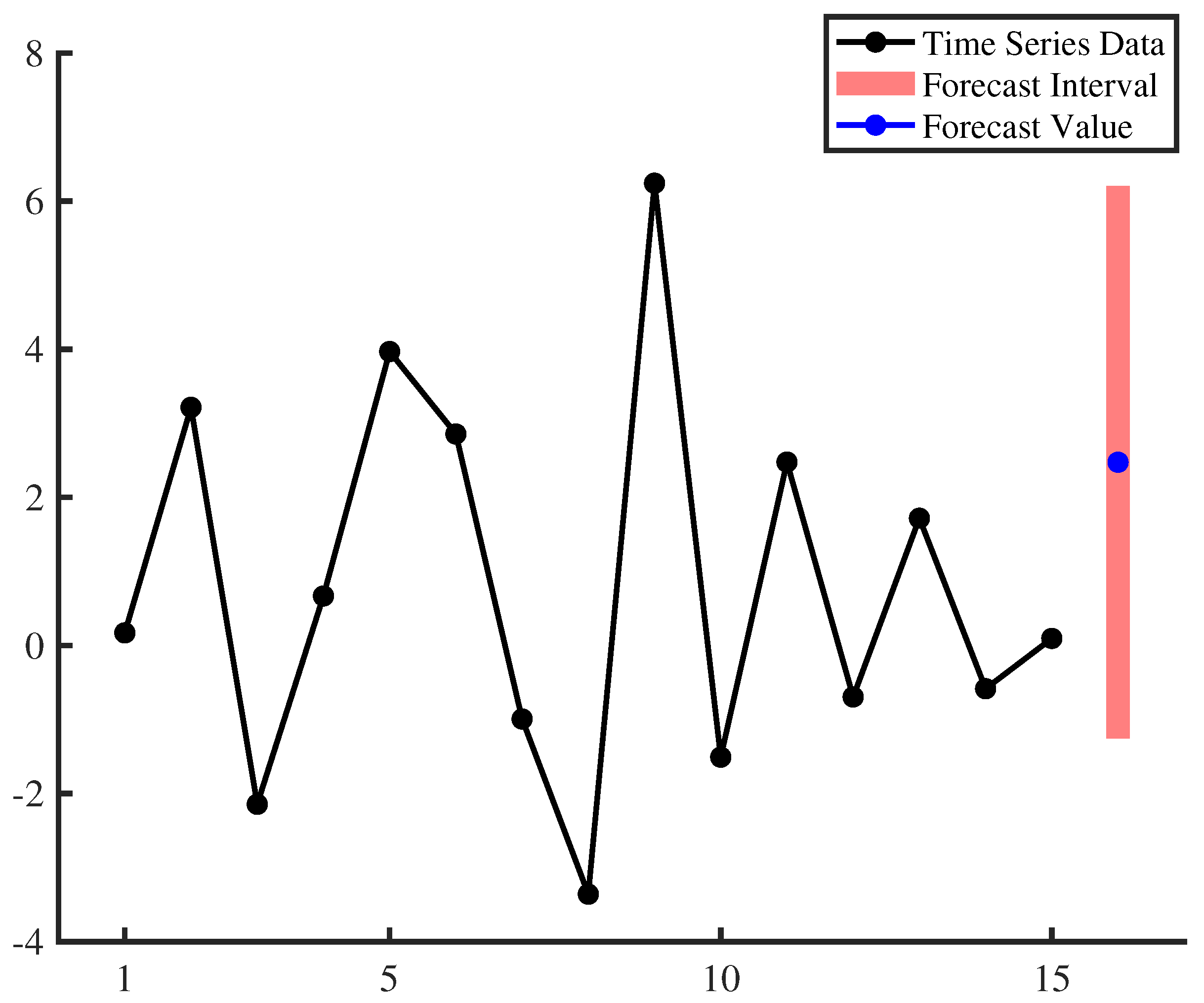
Finally, based on the estimated 1 order uncertain moving average model (15), we make a forecast of the time series data at the next moment, i.e., forecast $X_{16}$. On the basis of Equation (11), the forecast uncertain variable of $X_{16}$ can be calculated by

$${\widehat{X}}_{16}=0.9357-\sum _{i=1}^{15}{1.2114}^i\left(X_{16-i}-0.9357\right)+\mathcal{N}(0,1.8473).$$

(16)

Then, it follows from (12) and (13) that the forecast value of $X_{16}$ is

$$\widehat{\mu }=0.9357-\sum _{i=1}^{15}{1.2114}^i\left(X_{16-i}-0.9357\right)=2.4745,$$

and the $1-\alpha$ confidence interval is

$$2.4745\pm {\displaystyle \frac{1.8473\sqrt{3}}{\pi }}ln{\displaystyle \frac{1+\alpha }{1-\alpha }}=[-1.2567,6.2057].$$

By putting time series data, forecast value and forecast interval in the same graph (please see Figure 1), it can be seen that point forecast and interval forecast based on the estimated 1 order uncertain moving average model (15) can effectively inherit the trend of existing data and produce an effective forecast.

Furthermore, given that only moment estimation (proposed by Liu and Liu [26]) has been studied among the parameter estimation methods of uncertain moving average models based on uncertainty theory, here we apply the moment estimation method based on the same dataset shown in Table 1 to compare with the method proposed in this paper. It follows from the work of Liu and Liu [26] that the moment estimations of $a_0$, $a_1$, and $\sigma$ should solve the following system of equations:

$$\left\{\begin{array}{cc}{\displaystyle \frac{1}{15}\sum _{t=1}^{15}\frac{{\displaystyle X_t-a_0+\sum _{i=1}^{t-1}{a}_1^i\left(X_{t-i}-a_0\right)}}{\sigma }=0}\hfill & \\ {\displaystyle \frac{1}{15}\sum _{t=1}^{15}{\left(\frac{{\displaystyle X_t-a_0+\sum _{i=1}^{t-1}{a}_1^i\left(X_{t-i}-a_0\right)}}{\sigma }\right)}^2=1}\hfill & \\ {\displaystyle \frac{1}{15}\sum _{t=1}^{15}{\left(\frac{{\displaystyle X_t-a_0+\sum _{i=1}^{t-1}{a}_1^i\left(X_{t-i}-a_0\right)}}{\sigma }\right)}^3=0.}\hfill \end{array}\right.$$

By using Matlab to solve the above system of equations, we obtain

$${\widehat{a}}_0=0.8814,{\widehat{a}}_1=-0.6262,\widehat{\sigma }=4.0660.$$

Thus, the estimated 1 order uncertain moving average model by moment estimation method is obtained as

$$\begin{array}{c}\hfill X_t=0.8814+{ϵ}_t+0.6262{ϵ}_{t-1},\end{array}$$

(17)

where ${\epsilon }_t$, $t=1,2,\cdots$ are a set of uncertain disturbance terms and are assumed to obey the normal uncertainty distribution $\mathcal{N}(0,4.0660)$. It can be seen from the estimated models (17) and (15) that the standard deviation of the residuals estimated based on the moment estimation method is 4.0660, which is much larger than the standard deviation of the residuals estimated based on the least squares method, which is 1.8473. This indicates that the residuals estimated based on the moment estimation method still contain a large amount of uncertainties, and its prediction accuracy is much worse than the method proposed in this paper. On the other hand, we can also calculate the mean absolute error (MAE) and mean square error (MSE) of these two estimated models based on the dataset shown in Table 1, as shown in

Table 3. MAEs and MSEs of the estimated uncertain moving average models (15) and (17) using least squares method and moment estimation method.

	MAE	MSE
least squares method	1.2710	2.2534
moment estimation method	3.5640	16.5320

, respectively. It can also be seen from Table 3 that the prediction error of the least squares method proposed in this paper is much smaller than that of the moment estimation method, which fully demonstrates the effectiveness of the method proposed in this paper.

7. Real Data Example

In this section, we will provide a real data example to illustrate the proposed parameter estimation methods and the model testing and forecast methods, in which the dataset is global daily carbon dioxide emission per day during 1 July 2023 to 31 July 2023 and was collected by Liu and Liu [26], as shown in

Table 4. Global daily carbon dioxide emission per day during 1 July 2023 to 31 July 2023.

93.65	90.26	93.97	94.63	93.54	96.45	96.29	95.08	92.23
94.65	96.25	97.26	98.5	97.6	95.98	93.35	96.26	100.01
100.01	100.25	100.06	97.26	93.27	96.14	98.79	98.85	97.26
96.11	94.61	90.72	93.87

. In the work of Liu and Liu [26], the 3 order uncertain moving average model was obtained as

$$\begin{array}{c}\hfill X_t=96.257+{ϵ}_t+0.785{ϵ}_{t-1}+0.026{ϵ}_{t-2}-0.392{ϵ}_{t-3},\end{array}$$

(18)

where ${\epsilon }_t$, $t=1,2,\cdots$ are a set of uncertain disturbance terms and are assumed to obey the normal uncertainty distribution $\mathcal{N}(0,3.494)$.

Next, we will describe the above time series data in Table 4 based on the 3 order uncertain moving average model and the least squares estimation method, and carry out corresponding research on parameter estimation, model testing and forecast. For the 3 order uncertain moving average model, it is easy to infer that

$${\pi }_0=1,{\pi }_i=\sum _{j=1}^{3\wedge i}{a}_j{\pi }_{i-j},i=1,2,\cdots$$

Thus, it follows from the constructed statistical invariants (6) that we can obtain 31 real functions $h_1,h_2,\cdots ,h_{31}$ as

$$h_t(a_0,a_1,a_2,a_3,\sigma )={\displaystyle \frac{{\displaystyle X_t-a_0+\sum _{i=1}^{t-1}{\pi }_i\left(X_{t-i}-a_0\right)}}{\sigma }},t=1,2,\cdots ,31$$

by substituting the time series data from Table 4. Then, according to minimization problem (8), the least squares estimations of $a_0$, $a_1$, $a_2$, $a_3$, and $\sigma$ should solve the following minimization problem:

$$\begin{array}{cc}\hfill & \underset{a_0,a_1,a_2,a_3,\sigma >0}{min}\sum _{t=1}^{31}{\left({\left(1+exp\left({\displaystyle \frac{-\pi h_t}{\sqrt{3}}}\right)\right)}^{-1}-{\displaystyle \frac{1}{31}}\sum _{j=1}^{31}\mathbb{I}(h_j\le h_t)\right)}^2.\hfill \end{array}$$

By using Matlab to solve the above optimization problem, we obtain

$${\widehat{a}}_0=95.5417,{\widehat{a}}_1=0.0701,{\widehat{a}}_2=-0.6170,{\widehat{a}}_3=0.0880,\widehat{\sigma }=3.0614.$$

Thus, the estimated 3 order uncertain moving average model is obtained as

$$\begin{array}{c}\hfill X_t=95.5417+{ϵ}_t-0.0701{ϵ}_{t-1}+0.6170{ϵ}_{t-2}-0.0880{ϵ}_{t-3},\end{array}$$

(19)

where ${\epsilon }_t$, $t=1,2,\cdots$ are a set of uncertain disturbance terms and are assumed to obey the normal uncertainty distribution $\mathcal{N}(0,3.0614)$. It can be seen from the estimated models (18) and (19) that the standard deviation of the residuals estimated based on the moment estimation method is 3.494, which is much larger than the standard deviation of the residuals estimated based on the least squares method, which is 3.0614. This indicates that the residuals estimated based on the moment estimation method still contain a large amount of uncertainties, and its prediction accuracy is much worse than the method proposed in this paper.

Next, we will combine the time series data in Table 4 to test the estimated 3 order uncertain moving average model (19) to evaluate whether it is suitable. By substituting the 31 time series data and the estimated parameters ${\widehat{a}}_0$, ${\widehat{a}}_1$, ${\widehat{a}}_2$, ${\widehat{a}}_3$, and $\widehat{\sigma }$ into (5) and then using

$${\epsilon }_t=X_t-95.5417+\sum _{i=1}^{t-1}{\pi }_i\left(X_{t-i}-95.5417\right),t=1,2,\cdots ,31,$$

we can obtain 31 residuals data ${\epsilon }_1,{\epsilon }_2,\cdots ,{\epsilon }_{31}$ as shown in

Table 5. Residuals data of estimated 3 order uncertain moving average model (19).

−1.8917	−5.4142	−0.7838	2.2074	−1.8399	−0.6516	2.0321	−0.0793	−4.6284
−0.9882	3.4878	2.1650	0.8711	1.0904	0.1678	−2.7761	0.5163	6.2320
4.3421	1.2128	2.4727	1.5254	−3.5837	−0.3763	5.5673	3.6151	−1.4965
−1.2771	0.2203	−4.1500	−2.2108

. Suppose we consider the suitability test of the estimated 3 order uncertain moving average model (19) with a significance level of $\alpha =0.05$. Then, it follows from $\alpha \times 31=1.55$ and Equation (10) that the test is

$$\begin{array}{cc}\hfill W=\{({\epsilon }_1,{\epsilon }_2,\cdots ,{\epsilon }_{31}):& \mathrm{there} \mathrm{are} \mathrm{at} \mathrm{least} 2 \mathrm{of} \mathrm{indexes}{t}^{\prime }\mathrm{s} \mathrm{with}1\le t\le 31\hfill \\ \hfill & \mathrm{such} \mathrm{that}{\epsilon }_t<-6.1836 \mathrm{or} {\epsilon }_t>6.1836\}.\hfill \end{array}$$

As shown in Table 5, we can verify that only ${\epsilon }_{18}\notin [-6.1836,6.1836]$. Therefore, we have

$$({\epsilon }_1,{\epsilon }_2,\cdots ,{\epsilon }_{31})\notin W.$$

That is, according to the relevant results of the previous model test, we can reach the conclusion that the estimated 3 order uncertain moving average model (19) has a good fit to the time series data in Table 4 and is reasonable.

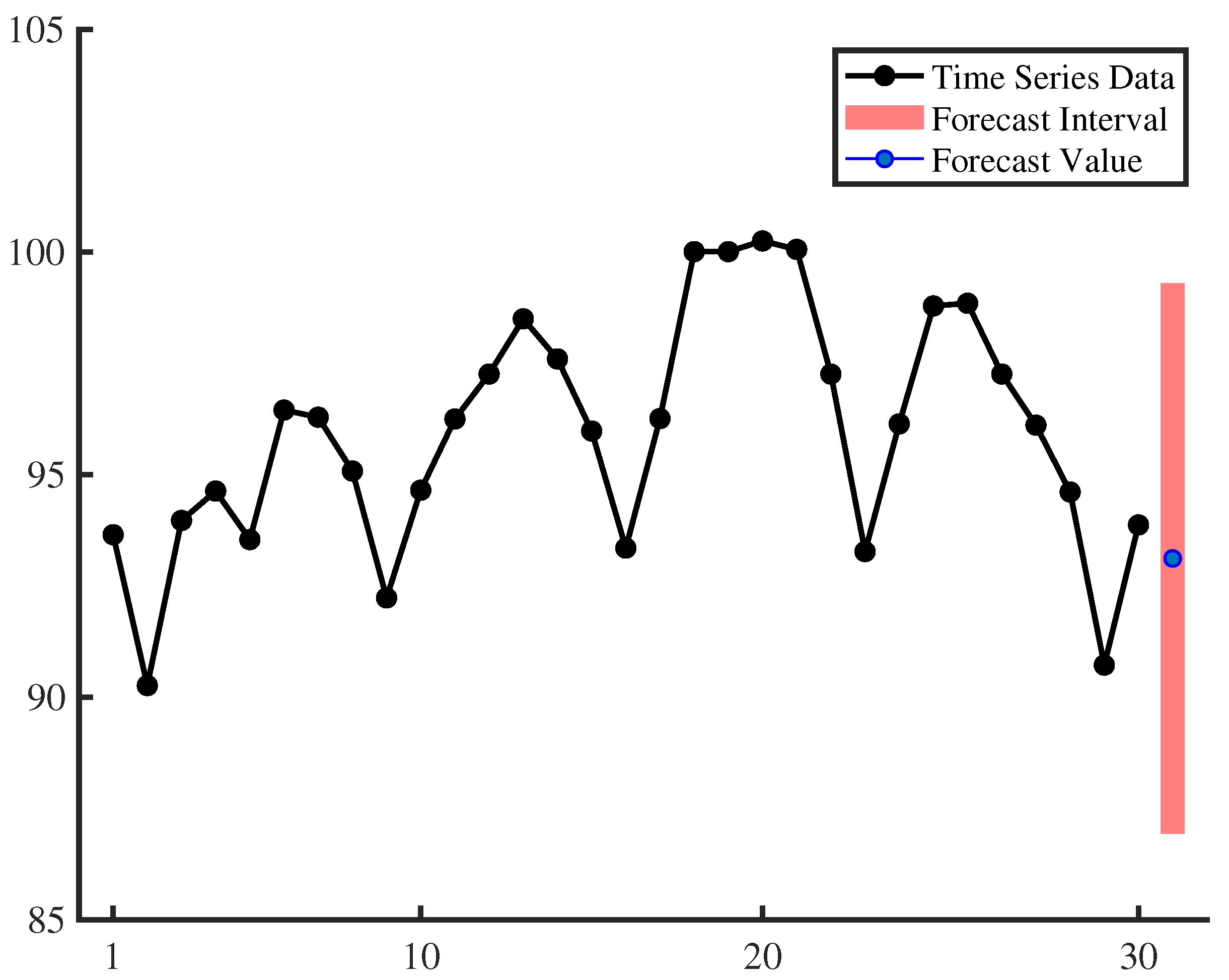
Finally, based on the estimated 3 order uncertain moving average model (19), we make a forecast of the time series data at the next moment, i.e., forecast $X_{32}$. On the basic of Equation (11), the forecast uncertain variable of $X_{32}$ can be calculated by

$${\widehat{X}}_{32}=95.5417-\sum _{i=1}^{31}{\pi }_i\left(X_{31-i}-95.5417\right)+\mathcal{N}(0,3.0614).$$

(20)

Then, it follows from (12) and (13) that the forecast value of $X_{31}$ is

$$\widehat{\mu }=95.5417-\sum _{i=1}^{31}{\pi }_i\left(X_{31-i}-95.5417\right)=93.1167,$$

and the $1-\alpha$ confidence interval is

$$93.1167\pm {\displaystyle \frac{3.0614\sqrt{3}}{\pi }}ln{\displaystyle \frac{1+\alpha }{1-\alpha }}=[86.9331,99.3003].$$

By putting time series data, forecast value and forecast interval in the same graph (please see Figure 2), it can be seen that point forecast and interval forecast based on the estimated 3 order uncertain moving average model (19) can effectively inherit the trend of existing data and produce an effective forecast.

8. Conclusions

In order to solve and enrich the research of statistical inference of the uncertain moving average model, a new method was proposed in this paper by deforming the uncertain moving average model to construct a symmetric statistical invariant, the normal uncertain variable. Based on this, the unknown parameters and uncertain disturbance terms in the uncertain moving average model were also determined by estimating the unknown parameters in the statistical invariants based on the least square principle. In addition, a numerical algorithm was designed to calculate the corresponding estimates. Then, this paper used the uncertain hypothesis test to verify the applicability of the estimated uncertain moving average model, discussed how to make point forecast and interval forecast for the future value of time series based on the estimated uncertain moving average model. Finally, a numerical example study was given to illustrate the proposed method and compared with existing methods to illustrate the advantages of the proposed method.