Article

The Effect of Graphene Nanofiller on Electromagnetic-Related Primary Resonance of an Axially Moving Nanocomposite Beam

1
Department of Aerospace Engineering, Chongqing University, Chongqing 400044, China
2
Faculty of Arts and Sciences, Beijing Normal University, Zhuhai 519087, China
3
State Key Laboratory of Mountain Bridge and Tunnel Engineering, Chongqing Jiaotong University, Chongqing 400074, China
*
Authors to whom correspondence should be addressed.
Symmetry 2025, 17(5), 651; https://doi.org/10.3390/sym17050651
Submission received: 27 February 2025 / Revised: 8 April 2025 / Accepted: 18 April 2025 / Published: 25 April 2025
(This article belongs to the Special Issue Symmetry in Graphene and Nanomaterials)

Abstract

:
The primary resonance responses of high-performance nanocomposite materials used in spacecraft components in complex electromagnetic field environments were investigated. Simultaneously considering the interfacial effect, agglomeration effect, and percolation threshold, a theoretical model that can predict Young’s modulus and electrical conductivity of graphene nanocomposites is developed by the effective medium theory (EMT), shear lag theory, and the Mori-Tanaka method. The magnetoelastic vibration equation for an axially moving graphene nanocomposite current-carrying beam was derived via the Hamilton principle. The amplitude-frequency response equations were obtained for different external loading conditions. The study reveals the significant role of graphene concentration, external force, and magnetic field on the system’s primary resonance, highlighting how electromagnetic forces play a critical role similar to external excitation forces. It is shown that the increase in graphene content could lead the system from period-doubling motion into chaotic behavior. Moreover, an enhanced magnetic field strength may lower the minimum graphene concentration needed for period-doubling motion. This work provides new insights into controlling nonlinear vibrations of such systems through applied electromagnetic fields, emphasizing the importance of designing multifunctional nanocomposites in multi-physics coupled environments. The concentration of graphene filler would significantly affect the primary resonance and bifurcation and chaos behaviors of the system.

1. Introduction

The evolution of lightweight multifunctional nanocomposites plays a pivotal role in propelling next-generation material innovations. Recent advancements highlight graphene-enhanced composites as transformative solutions across interdisciplinary domains, including intelligent robotic actuators [1,2], automotive electrification systems [3], and aerospace structural components [4,5], demonstrating unparalleled multifunctional synergy. Axially mobile graphene-reinforced beams, serving as critical elements in advanced mechanical systems, necessitate rigorous investigation into their dynamic stability under multi-physics coupled environments involving concurrent mechanical-electromagnetic interactions. This study establishes a theoretical framework for governing nonlinear vibrations through strategic electromagnetic field modulation.
Polymer matrices, notably epoxy systems, demonstrate exceptional enhancements in mechanical and conductive properties through the integration of high-performance graphene nanofillers. Empirical studies reveal that 9% graphene loading achieves a 271.8% modulus amplification relative to pristine matrices [6], while 2% filler concentration elevates conductivity to 10 9 S/m-a nine-order-of-magnitude improvement over insulating polymers [7]. This dual reinforcement mechanism leverages graphene’s nanoscale stress transfer capability and electron tunneling networks.
A spectrum of micromechanical approaches has been formulated to characterize composite material properties, encompassing shear lag theory [8,9,10], Halpin-Tsai semi-empirical models [11,12], Eshelby’s inclusion-based formulations [13], Mori-Tanaka mean-field homogenization [14,15], self-consistent schemes [16], and Hashin-Shtrikman variational bounds [17]. While these methodologies incorporate constituent phase attributes and morphological descriptors, their isolated application impedes comprehensive modeling of interfacial coupling phenomena spanning filler-matrix adhesion and filler-filler percolation networks, particularly for graphene agglomeration dynamics and critical conductivity thresholds. Weng’s pioneering equivalent medium approximation (EMA) [18] leverages Maxwell’s far-field equivalence principle, enhanced through interfacial phase modeling [7,19,20], to evaluate nanocomposite transport properties. The Mori-Tanaka framework, though proficient in predicting coated nanofiller effective properties, overlooks interfacial stress discontinuity effects. Conventional shear lag analyses, despite successfully correlating filler geometry (via Krenchel orientation factors) with macroscopic elastic enhancement, neglect three pivotal aspects: (1) interfacial shear stress redistribution mechanisms, (2) surfactant-mediated interfacial plasticity, and (3) temporal evolution of agglomerate morphology.
Despite substantial progress in theoretical modeling, critical knowledge gaps persist in elucidating the synergistic interplay between graphene nanofiller aggregation kinetics and polymer-filler interfacial thermodynamics, particularly under dynamic multi-physics coupling conditions. Recent advances in the nonlinear dynamics of graphene nanocomposite beams have unveiled complex behavioral patterns under multifield interactions, necessitating sophisticated analytical frameworks. Wang et al. [21] pioneered a multiphysics-coupled theoretical-numerical paradigm for dielectric graphene-reinforced beams, integrating equivalent medium theory with Timoshenko beam kinematics and geometrically nonlinear Von Kármán strain formulations to holistically evaluate Young’s modulus, dielectric permittivity, and mass density through generalized mixture rules. Their differential integration methodology established a benchmark for predicting nonlinear free vibration modes under electric field perturbations. Li et al. [22] developed a multiscale asymptotic framework to deconvolute resonance characteristics in functionally graded polymer beams, demonstrating through parametric sweeps that ultralow graphene loadings (0.1–0.5 wt.%) with square platelet architectures maximally attenuate combined harmonic-subharmonic resonance amplitudes by 63–78%. Gholami and Ansari’s groundbreaking work [23] employed a hybrid Galerkin-temporal discretization scheme augmented with pseudo-arclength continuation, revealing magnetic flux density-dependent bifurcation phenomena in graded beams and quantifying nonlinear stiffness modulation under 10–30 T fields. Song et al. [24,25] systematically mapped thermal gradient effects on vibration modes of GNP-distributed beams via high-order differential quadrature methods, identifying a critical temperature threshold beyond which agglomeration-induced mode localization dominates. Wei’s innovative variational Padé synthesis [26] resolved frequency-domain nonlinearities in lumped-parameter models, uncovering multiple coexisting natural frequencies through iterative amplitude-phase corrections. Vila’s inertia gradient continuum formulation [27] captured intrinsic scale effects across linear and nonlinear regimes, providing a unified framework for nano-to-meso transition modeling. Complementarily, Jalaei’s viscoelastic-porous coupling analysis [28] deciphered transient response phase transitions in magnetic-field-embedded graded nanobeams, establishing time-scale dependencies between porosity dissipation and Lorentz force dynamics. Despite these methodological leaps, the stability boundaries and primary resonance mechanisms governing axially translating current-carrying graphene beams under extreme magnetic fields remain critically underexplored, particularly regarding electromagnetic-elastic coupling hysteresis and strain rate-dependent damping effects.
This study establishes a unified theoretical framework by integrating interfacial electromechanical coupling effects through the synergistic application of shear lag mechanics and Mori-Tanaka homogenization within the EMT paradigm, with graphene filler aggregation dynamics and percolation transitions rigorously characterized via Cauchy statistical accumulation functions. The equivalent mechanical-electrical properties of epoxy-graphene composites are systematically determined across varying filler concentrations, enabling the formulation of magnetoelastic governing equations for axially moving current-carrying beams through Hamiltonian variational principles that explicitly incorporate geometric nonlinearities inherent to nanocomposite deformation. Under simply supported boundary conditions and first-order modal assumptions, analytical solutions of the dimensionless nonlinear vibration equations are derived via spacetime decoupling through Galerkin-weighted residual methods, followed by a comprehensive parametric sensitivity analysis to evaluate dynamic stability thresholds. The amplitude-frequency response equations are subsequently established to characterize primary resonance behaviors under multifield loading configurations, including isolated mechanical excitation, pure electrical stimulation, and coupled electromechanical interactions. Numerical investigations further unravel the regulatory mechanisms of external excitation force amplitude, current density intensity, magnetic flux density magnitude, and graphene volume fraction on resonance amplitude modulation, culminating in bifurcation topology maps that delineate graphene concentration-dependent stability transitions under graded magnetic field intensities.

2. Theory

2.1. Theoretical Modeling of Graphene Nanocomposites

2.1.1. Theoretical Framework of Effective Medium Theory

First, we consider a finite unit that contains a two-phase material consisting of a matrix denoted by subscript m, and an ellipsoidal inclusion denoted by subscript f. The modulus tensor L m and L f , can be replaced, respectively, with elastic modulus E, thermal conductivity tensor κ , electrical conductivity tensor σ , and permittivity tensor ε , etc. The corresponding volume concentrations for the matrix and the reinforcement phase are denoted as c m and c f , respectively. This unit is then embedded in a reference medium with a modulus denoted as L r . In contrast, an equivalent composite unit with the same size and homogeneity but an unknown modulus denoted as L e is also placed within the same reference medium L r . Low-frequency planar compression waves with wavelengths significantly larger than the dimensions of the filler u = u 0 x e i ω t are simultaneously applied to the left side of both models. Theoretical analysis is then performed for each model to study the scattered fields produced by these waves. The expression for the equivalent medium theory can be derived based on the equivalence condition of the Maxwell far-field matching method [18], which states that the volume average of the scattered field from all component phases in the composite material at a distance should be equivalent to the scattered field of the equivalent medium. Since the spatial orientation of the reinforcing phase is completely random, via the simplified treatment, L e can be characterized by a single value L e . By performing a spatial orientation average on the equivalent modulus tensor of the composite and simplifying the analysis, an expression can be derived for L e that satisfies the following criteria:
c m ( L m L e ) L e + S m ( L m L e ) + c f 3 2 ( L f 1 L e ) L e + S f 1 ( L f 1 L e ) + ( L f 3 L e ) L e + S f 3 ( L f 3 L e ) = 0
where S i is the depolarization tensor (Eshelby tensor) associated with the shape of component i [29]. The modulus tensor L m and Eshelby tensor S m of the matrix can be characterized by single values L m , and S m , respectively, based on their isotropic property. Similarly, the filler, which possesses in-plane symmetry, can have its modulus tensor L f and Eshelby tensor S f simplified to two independent components: L f 1 = L f 2 , L f 3 , S f 1 = S f 2 , S f 3 . The components of the Eshelby tensor S f are solely dependent on the thickness-to-diameter ratio of the filler, represented by α = λ / l (where λ is the thickness and l the diameter of the filler) [30]:
S f 1 = S f 2 = α 2 ( 1 α 2 ) 3 2 arccos α α α 2 1 1 2 , α < 1 α 2 ( α 2 1 ) 3 2 α 1 α 2 1 2 arcosh α , α > 1 S f 3 = 1 2 S f 2
Hence, given the filler geometries ( λ and l) and volume concentration ( c f ), we can replace the modulus tensor in Equation (1) with Young’s modulus or conductivity tensor, i.e., L E , L σ , to predict the equivalent mechanical and electrical properties of graphene nanocomposites.
c m ( E m E e ) E e + S m ( E m E e ) + c f 3 2 ( E f 1 E e ) E e + S f 1 ( E f 1 E e ) + ( E f 3 E e ) E e + S f 3 ( E f 3 E e ) = 0 c m ( σ m σ e ) σ e + S m ( σ m σ e ) + c f 3 2 ( σ f 1 σ e ) σ e + S f 1 ( σ f 1 σ e ) + ( σ f 3 σ e ) σ e + S f 3 ( σ f 3 σ e ) = 0

2.1.2. Interface, Agglomeration and Percolation Effects

Defects are commonly present in the vicinity of graphene nanocomposite interfaces, leading to various issues such as poor mechanical conditions, weak bond connections, thermal expansion mismatch, and phonon scattering. In general, the predictions made by classical micromechanical theories tend to overestimate the observed experimental results [31]. As a result, it is necessary to consider the effects of imperfect interfaces to accurately determine the intrinsic Young’s modulus and electrical conductivity of the nanomaterials where the filler can be treated as an inclusion consisting of an outer thin interfacial layer and an inner graphene filler. To determine the effective Young’s modulus of this inclusion E coa 1 , 3 , shear lag theory [32] is employed, and detailed derivation can be found in Wang et al. [33]. Similarly, Mori-Tanaka method is utilized to calculate the effective conductivity of this inclusion σ coa 1 , 3 [30].
E coa 1 , 3 = E f 1 , 3 E f 1 E int 1 V f + α 2 η 0 12 ( 1 + ν int ) V f σ coa 1 , 3 = σ int 1 + ( 1 V int ) ( σ f 1 , 3 σ int ) V int S f 1 , 3 σ f 1 , 3 σ int + σ int
where ν int is the Poisson’s ratio of the interfacial layer, η 0 is taken as 8/15 for the nanosheet filler with a completely random orientation [32], V f and V int denote the volume concentrations of the filler and the interfacial layer relative to the whole inclusions, respectively, and the sum of the two is 1. The expression of V f is as follows:
V f = λ 2 · λ 2 α 2 λ 2 + δ · λ 2 α + δ 2
where δ is the thickness of the interface layer and λ the thickness of the filler.
Assuming an extremely small thickness-to-diameter ratio of graphene, intimate contact between graphene layers is likely to occur, leading to the formation of agglomerated blocks and electrical current channels within the composite. The percolation threshold is typically defined as the graphene volume concentration at which the first electric current channel path forms [30]. To analyze the impacts of agglomeration and percolation effects on the mechanical and electrical properties of the interfacial layer of the graphene filler, we introduce Cauchy’s statistical cumulative function χ , with which the effective Young’s modulus [30,31] and electrical conductivity [7] of the interfacial layer are determined as follows:
E int = ζ E f χ ( c f , c f E , γ E ) + E m 1 χ ( c f , c f E , γ E ) σ int = σ int / χ ( c f , c f σ , γ σ )
where ζ denotes the interfacial coefficient between the reinforcement phase and the matrix [30,31,34], σ int the electrical conductivity of the interfacial layer as c f 0 . The Cauchy statistical cumulative function is defined as:
χ ( c f , c f E or σ , γ E or σ ) = F ( 1 , c f E or σ , γ E or σ ) F ( c f , c f E or σ , γ E or σ ) F ( 1 , c f E or σ , γ E or σ ) F ( 0 , c f E or σ , γ E or σ ) F ( c f , c f E or σ , γ E or σ ) = 1 2 + 1 π arctan c f c f E or σ γ E or σ
where c f E and c f σ denote the critical volume concentration at which agglomeration and percolation threshold occur, respectively, γ E and γ σ are scaling parameters that describe the variation in χ , F in the vicinity of c f E and c f σ , respectively, [7,35].

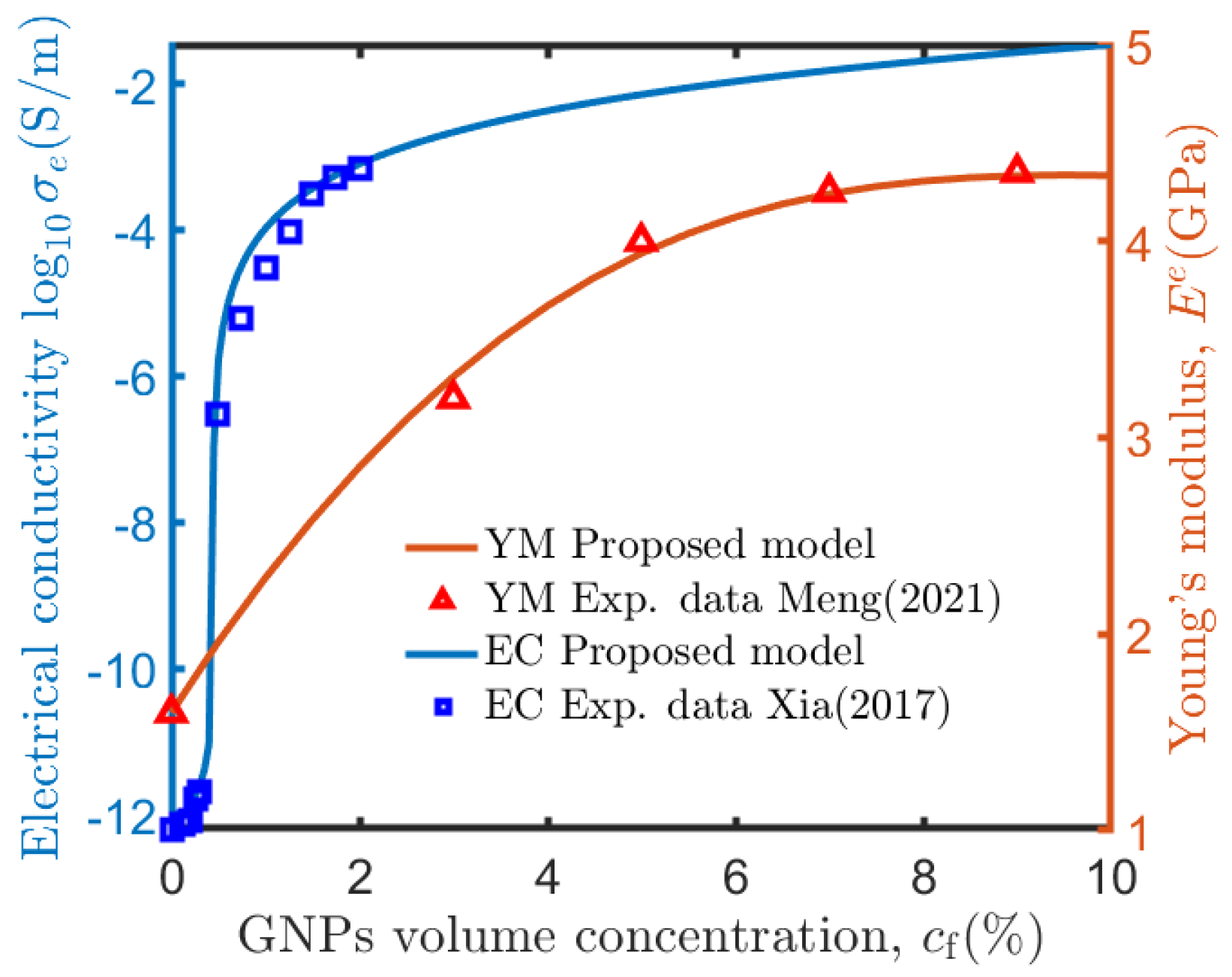
2.1.3. Model Verification

This study investigates the dependence of equivalent mechanical/electrical properties of graphene-epoxy nanocomposites on the filler volume concentration ( c f ) through a multiphysics-coupled model. Based on the previous research [36], the material parameters we use include the following: geometric properties of graphene nanosheets (thickness λ = 50.4 nm , interlayer thickness δ = 6.3 nm , length l = 2000 nm ); mechanical properties of constituents (polymer matrix Young’s modulus E m = 1.6 GPa , in-plane/out-of-plane graphene Young’s moduli E f 1 = 10 3 GPa / E f 3 = 2 GPa ); electrical properties (matrix conductivity σ m = 5.94 × 10 13 S/m, graphene in-plane/out-of-plane conductivities σ f 1 = 8.32   S / m / σ f 3 = 83.2   S / m ); and interfacial parameters (interface layer Poisson’s ratio ν int = 0.3 , zero-concentration interfacial conductivity σ int = 8.94 × 10 5   S / m , interface coupling coefficient ζ = 0.675 ). Critical parameters include agglomeration/percolation thresholds ( c f E = c f σ = 4 % ) and scaling factors for statistical accumulation functions ( γ E = 0.07 , γ σ = 4 × 10 5 ). As shown in Figure 1, the calculated equivalent modulus and conductivity align with experimental data from Meng et al. [6] and Xia et al. [7], quantitatively revealing the synergistic effects of interfacial interactions, agglomeration dynamics, and percolation thresholds on macroscopic composite properties.
The calculations of effective Young’s modulus and electrical conductivity of graphene-epoxy composites are plotted in Figure 1, where the experimental data by Meng et al. [6] and Xia et al. [7] are also given for comparison. In Figure 1 the red and blue lines (Proposed model) represent the calculated results when interfacial effects, agglomeration effects, and percolation threshold are taken into consideration simultaneously, and the red triangle and blue square are the experiment results of the graphene-epoxy composites’ Young’s modulus and electrical conductivity. It can be observed that these results closely align with the experimental data. Therefore, the predictions of the force-electric properties of the composite can be utilized for further studies.

2.2. Primary Resonance

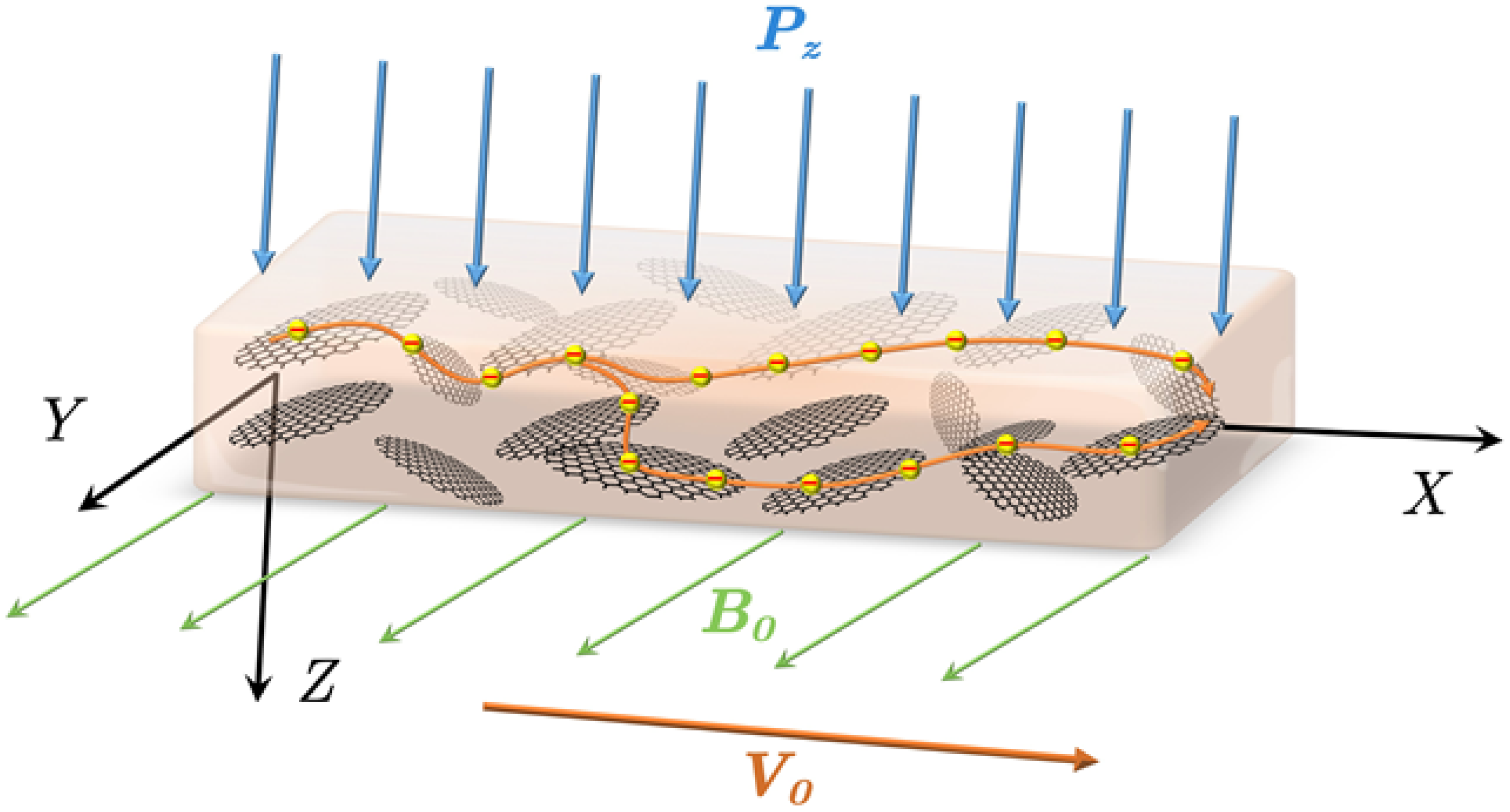
2.2.1. Model Setup and Vibration Equation

We investigate the dynamic behavior of an axially traveling conductive nanocomposite beam subjected to an orthogonal magnetic field B 0 = ( 0 , B 0 , 0 ) , characterized by an alternating current density J 0 = ( J 0 x , 0 , 0 ) and a distributed transverse harmonic force P z = f 0 sin ( ω 1 t ) , where f 0 denotes the force amplitude and ω 1 the angular excitation frequency. The beam, with geometric dimensions l (length), h (height), and b (width), features a rectangular cross-section A = b × h and translates along its longitudinal axis x at a constant velocity V 0 , as showed in Figure 2.
The beam theory we used was the Euler-Bernoulli beam theory, and the magnetoelastic vibration equation for the deflection of an axially moving current-carrying nanocomposite beam in a transverse magnetic field can be derived by considering linear elasticity, planar cross-section hypothesis and geometric nonlinearities based on Hamiltonian principle [37]:
ρ A 2 w t 2 + 2 ρ A V 0 2 w x t + ρ A V 0 2 2 w x 2 F 0 x 2 w x 2 3 2 E e A w x 2 2 w x 2 + E e I 4 w x 4 = A B 0 J 0 x σ e B 0 2 w t σ e B 0 2 V 0 w x + P z
Applying the vibration theory and utilizing the modal superposition technique, one can focus on the scenario where both ends ( x = 0 , l ) of the beam are pinned. By assuming a displacement solution that satisfies the boundary condition, one has w ( t , x ) = P ( t ) sin n π x / l . Then, we apply the Galerkin method. By separating the first-order resonance quantity, i.e., w ( t , x ) = P ( t ) sin π x / l component. Through integrating with sin π x / l , a similar process like Fourier transformation, we can derive the differential equation for the time-dependent coefficient P ( t ) of the first-order resonance. Furthermore, by adjusting the coefficient of the second-order derivative term to 1, and non-dimensionalize P ( t ) by dividing h, we arrive at the following non-dimensional transverse differential equation for vibration:
q ¨ + g 2 q = k 1 q ˙ 9 2 q 3 + k 2 sin ( Ω 1 τ ) + k 3 sin ( Ω 2 τ )
where
q = P h ; τ = ω n t ; Ω 1 = ω 1 ω n ; Ω 2 = ω 2 ω n ; k 1 = σ e B 0 2 ρ ω n ; k 2 = 4 f 0 ρ A ω n 2 π h ; k 3 = 4 B 0 j 0 ρ ω n 2 π h ; k 4 = V 0 l ω n ω n = E e I π 4 ρ A l 4 ; ξ = F 0 x l 2 E e I π 2 ; g 2 = 1 π 2 k 4 2 + ξ
The multi-scale perturbation technique is employed to analyze the primary resonance characteristics of the dynamical system. By introducing a dimensionless small parameter ε on the right-hand side of Equation (9) and expanding the generalized coordinate q = q ( τ , ε ) up to first-order terms, followed by elimination of secular terms, a coupled system of amplitude-phase modulation equations emerges, governing the evolution of complex amplitudes in the regime of interest [37].
a = k 1 2 a k 2 + k 3 2 g cos γ γ = ε σ 27 16 g a 2 + k 2 + k 3 2 g sin γ
Applying the stability condition ( a = 0 , γ = 0 ) to Equation (10), we obtain the amplitude-frequency response equation of the system,
k 1 2 4 + ε σ 27 16 g a 2 2 a 2 = ( k 2 + k 3 ) 2 4 g 2

2.2.2. Model Verification

This study focuses on the nonlinear vibration response of graphene nanocomposites in extreme deep-space environments, where ultrahigh magnetic fields are ubiquitous. Astronomical observations indicate that celestial bodies such as magnetars and pulsars exhibit surface magnetic fields reaching 10 10 T and internal fields up to 10 13 T [38]. Although achieving such fields in laboratories remains challenging, recent advances in no insulation high-temperature superconducting magnets validate experimental feasibility [39]. This study adopts 40 T as the baseline, balancing experimental accessibility and astrophysical relevance, to systematically investigate nonlinear vibrations of graphene nanocomposite beams, offering theoretical guidance for deep-space component design.
Figure 3 presents the dynamic response curve of the system using three different model assumptions, i.e., (1) MA1 (the blue dash-dot line), using the original EMT model; (2) MA2 (the green solid line), the EMT model while considering the interface effect; and (3) MA3 (the orange dash line), using the model proposed in the article. Making use of the singularity theory, the magnetic field-axial velocity and axial force-velocity singularity distributions of the three model parameters in a certain range are analyzed. Figure 3a is the magnetic field-axial velocity singularity diagram, and the results obtained from the calculations using different models are significantly different. However, in Figure 3b, the axial force-velocity singularity diagram, the curve obtained using MA3 is consistent with that using MA2. The green dots in Figure 3b are the intersections of dynamic response curves with the F 0 x = 0 line. Figure 3c,d demonstrate the first-order amplitude-frequency resonance curves of the system using the three model assumptions under different loading conditions (only excitation force is applied, and both force and current are applied), respectively. The interface effect, agglomeration effect, and percolation threshold play counteractive roles, leading to a noteworthy reduction in the primary resonance amplitude of the system. Thus, the theoretical model developed in this paper, which simultaneously considers the interface effect, agglomeration effect, and percolation threshold, effectively predicts the primary resonance response of axially moving graphene nanocomposite current-carrying beams in a magnetic field.
Assuming the axially moving current-carrying beam is made of copper with the main parameters as follows: l = 0.3 m, b = 0.02 m, and h = 0.01 m. It can be seen that the axial tension is F 0 x = 30 kN.

3. Numerical Calculation and Discussion

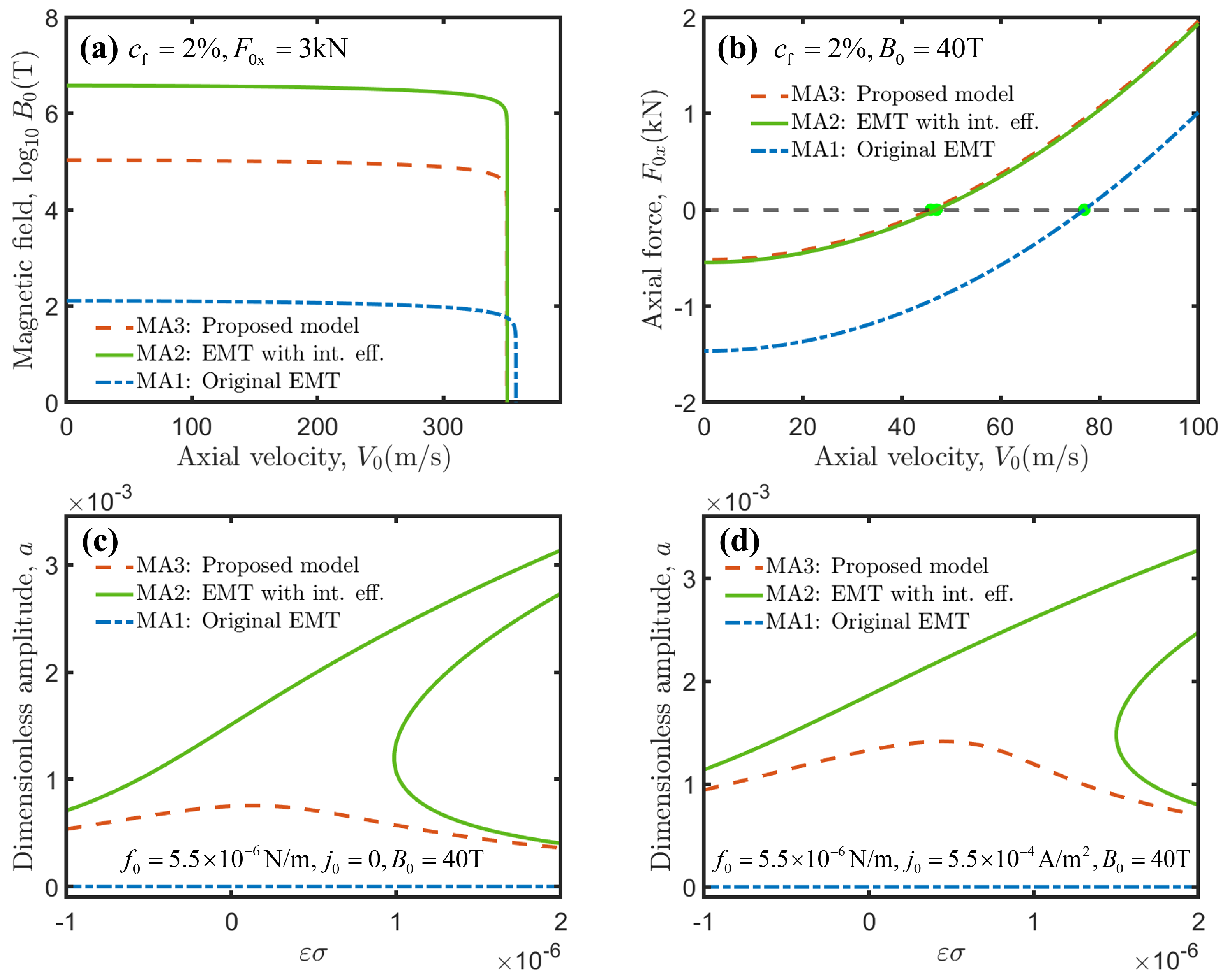
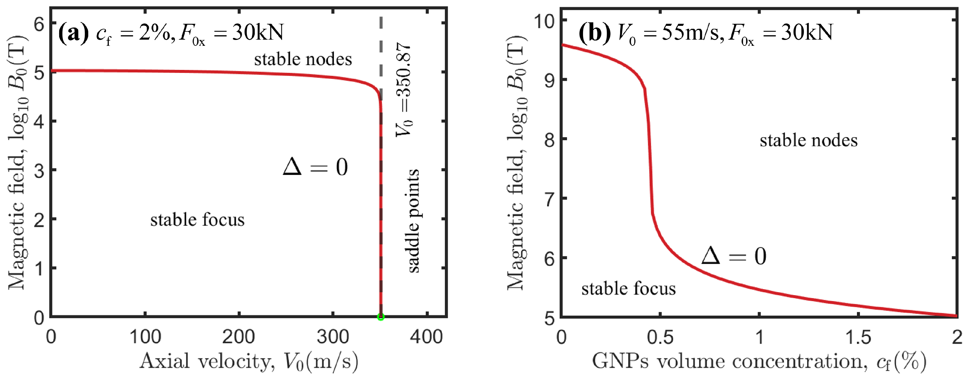
3.1. Stability Analysis

Utilizing singularity analysis theory [37], Figure 4 illustrates the singularities and the partitioning of stability areas based on the parameters within a specified range, in which the boundary domain discriminant is Δ = k 1 2 4 g 2 . It can be observed in Figure 4a that with the increase in axial velocity, the magnetic field associated with the boundary of the separated stable focus and stable nodes tends to decrease. When the velocity reaches a certain threshold, all singularities transition into saddle points, indicating that the distribution of singularities is highly influenced by the axial velocity. Figure 4b demonstrates that as the concentration of the graphene-enhanced phase increases, the magnetic field associated with the boundary between stable focus and stable nodes tends to diminish. The increase in the volume concentration of GNPs significantly increases the electric conductivity of the composite material and enhances the impact of the magnetic field on the structure, leading to a more stable vibration. Which, as shown in Figure 4b, results in the widened area of stable nodes. Additionally, as the concentration of the graphene filler continues to rise, no unstable region appears in the figure, indicating that the variation in the concentration of the graphene-enhanced phase has minimal influence on the stability of the system.

3.2. Primary Resonance

Primary resonance, a critical phenomenon in nonlinear systems triggered when external excitation frequencies approach natural frequencies, plays a decisive role in structural dynamic stability [40]. The nonlinear vibration behaviors of graphene nanocomposites under electromagnetic coupling exhibit exceptional complexity. This study integrates interfacial effects, agglomeration, and percolation within an effective medium theory framework, systematically elucidating primary resonance mechanisms of axially moving beams under 40 T magnetic fields, thereby offering novel insights for structural design in deep-space extreme environments [38]. In the figures below, the shadow means the multi-value region, and the dashed lines marked the turning GNPs volume concentration.

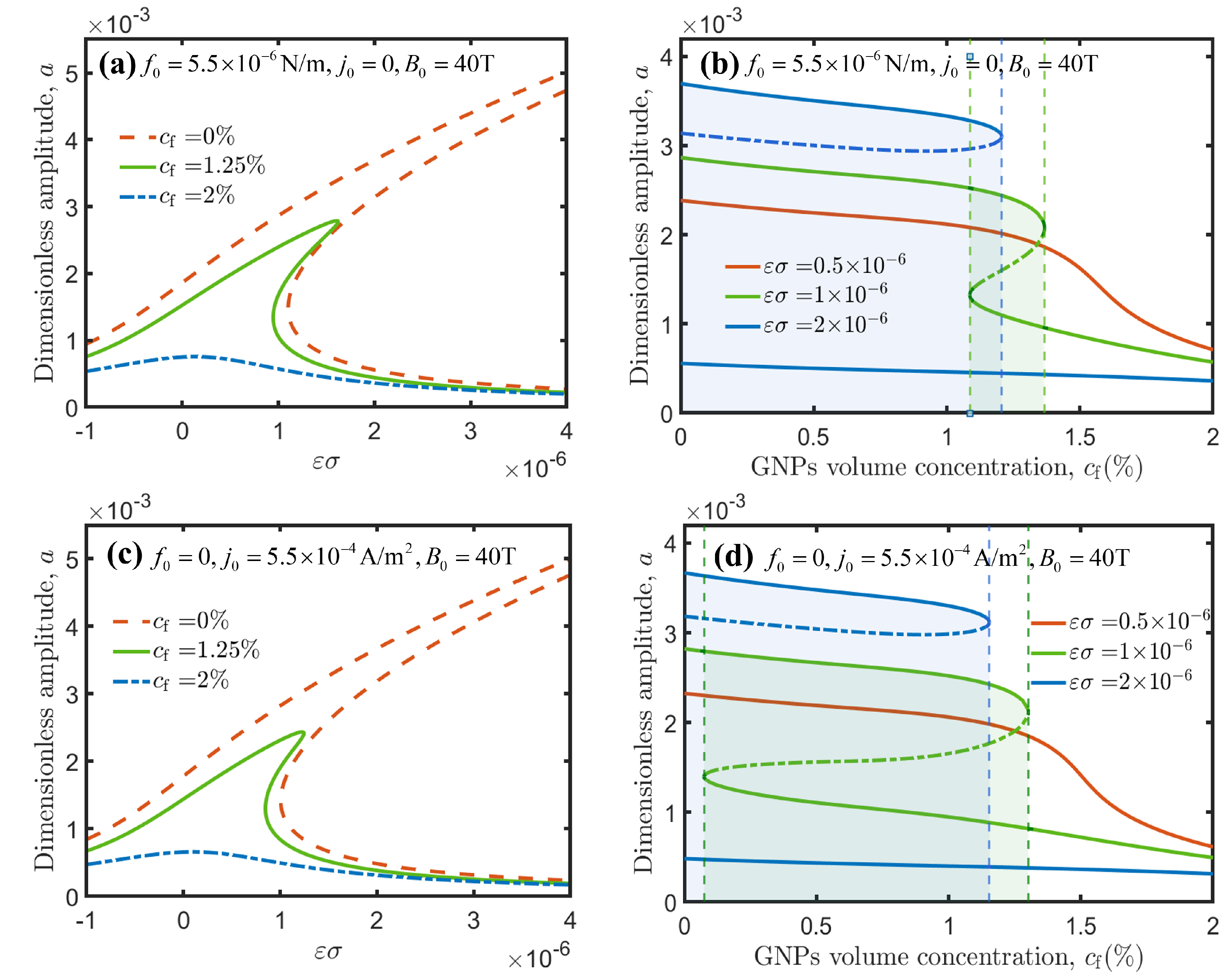
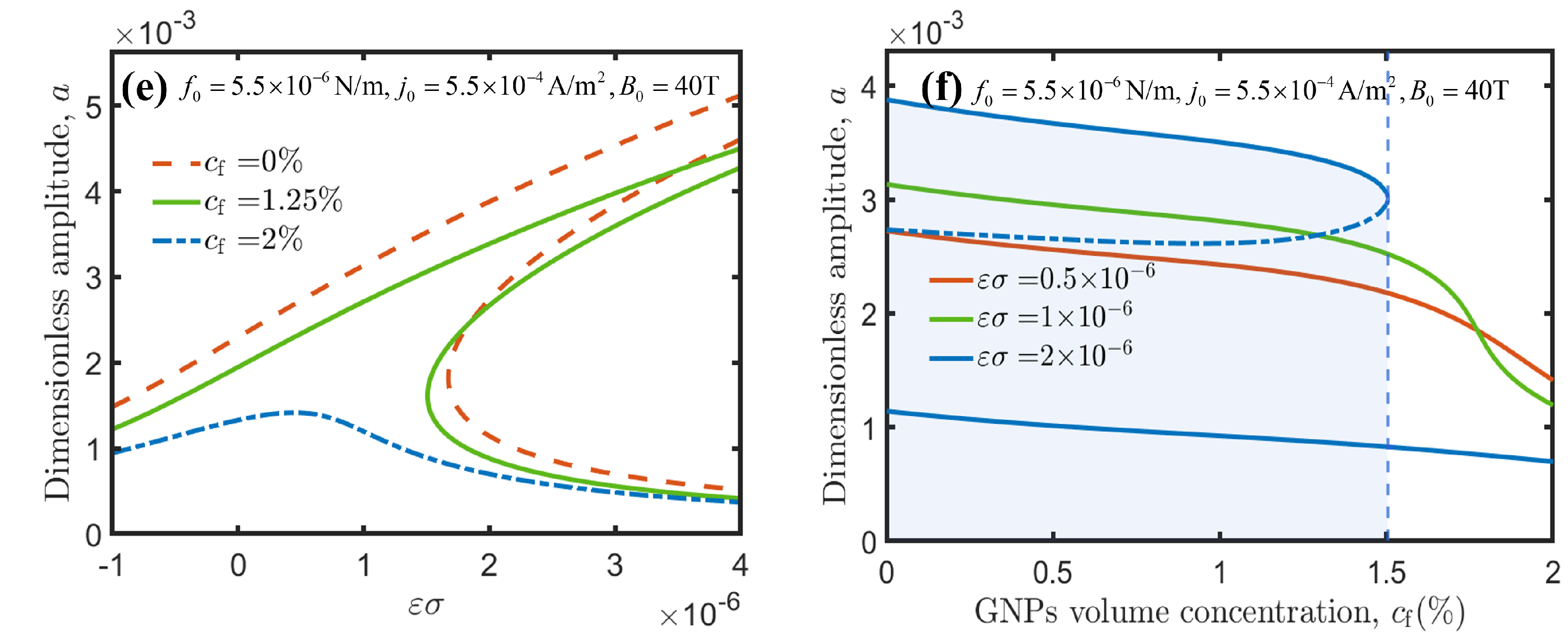
3.2.1. Amplitude-Frequency Response

Figure 5 shows the amplitude-frequency relationships and the corresponding amplitude-graphene concentration diagrams under different loading conditions, including excitation force [Figure 5a,b], external current [Figure 5c,d], and both external force and current [Figure 5e,f]. The x-axis, labeled as ε σ , means the tuning parameter of the frequency and is further discussed in Supplementary Materials. It is evident in Figure 5a,c that at low graphene volume concentrations, the system amplitude exhibits a region with multiple solutions (the orange dash line) as the tuning parameter increases; the amplitude decreases, and the region with multiple solutions becomes narrower and shifts to the left (the green solid line) as the concentration increases. When the graphene volume concentration reaches a certain value, the system amplitude has only a single-valued solution (the blue dash-dot line). In the case of combined external excitation force and external current (Figure 5e), a significant increase in amplitude is observed, and the multivalued region is significantly widened and shifted to the right. It indicates that in a strong magnetic field, both the increase in graphene concentration and the decrease in external load contribute to the reduction in the presence of multiple solutions in the amplitude. Furthermore, the tuning parameter has a significant impact on the extent of the region with multiple solutions (Figure 5b,d,f). With the increase in the tuning parameter, the region with multiple solutions widens considerably and shifts backward as a whole.

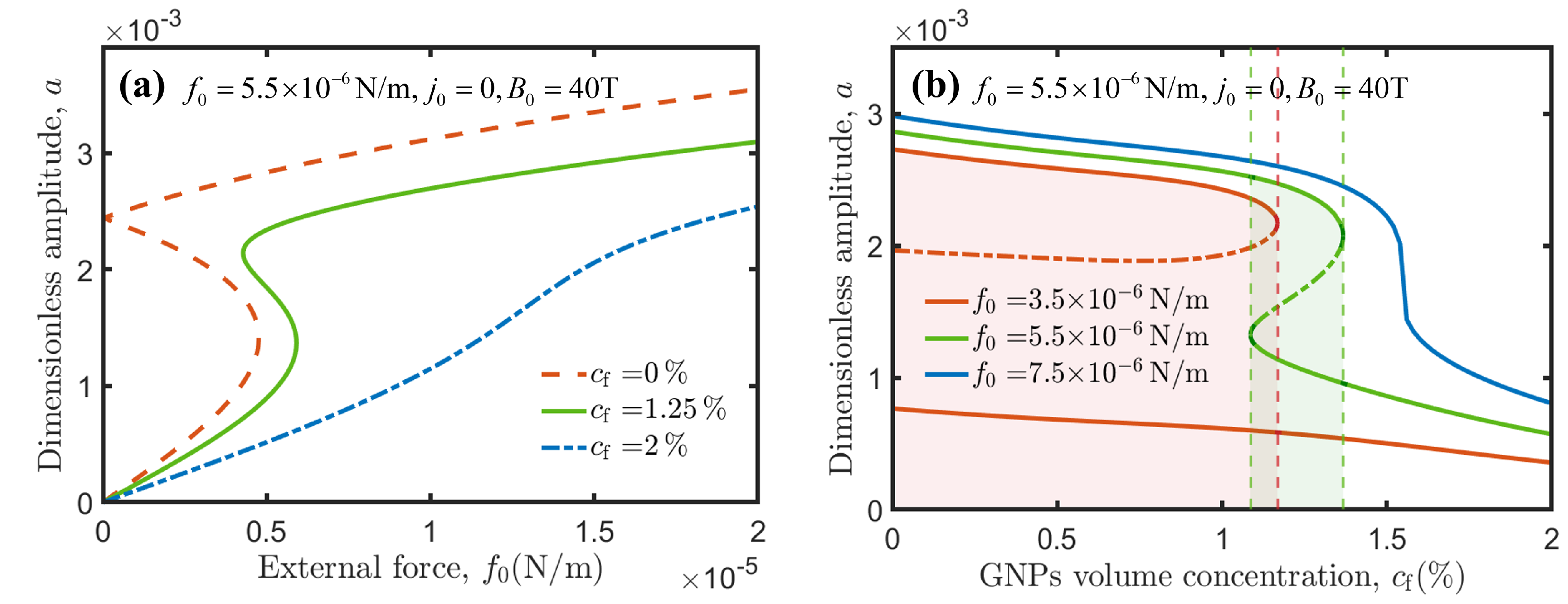
3.2.2. Amplitude-External Load Response

Figure 6 shows the amplitude-external load diagrams and the corresponding amplitude-graphene concentration diagrams under different external loading conditions, including LC1-external excitation force [Figure 6a,b], LC2-external current [Figure 6c,d] and LC3-both external force and the external current [Figure 6e,f]. Comparing Figure 6a and Figure 6c, the amplitude values of the two curves are close to each other, which indicates that the contribution of electromagnetic force to the nonlinear response of the system is not negligible in a strong magnetic field environment. From Figure 6a,c, it can be seen that the amplitude increases with the increase in the external excitation force amplitude and the external load current density. At lower concentrations, multivalued solutions exist in the interval where the external load effect is small; when the external load is larger than a certain value, the multivaluedness disappears. As the concentration increases, the curve gradually unfurls, resulting in a decrease in amplitude. Simultaneously, the region with multiple solutions narrows and shifts towards the right until it eventually vanishes. Moreover, as shown in Figure 6b,d the applied load significantly affects the range of the multi-value region of the system, and the multi-value region significantly narrows or even disappears with the increase in the applied load, and its position is shifted backward as a whole.
Figure 6e,f are the 3D and the vertical view of primary resonance diagrams under both the external excitation force and the load current. The intersection line between the surface and the plane at a = 0 is a straight line, indicating the equivalence between the external excitation force and the external load current under a fixed magnetic field.

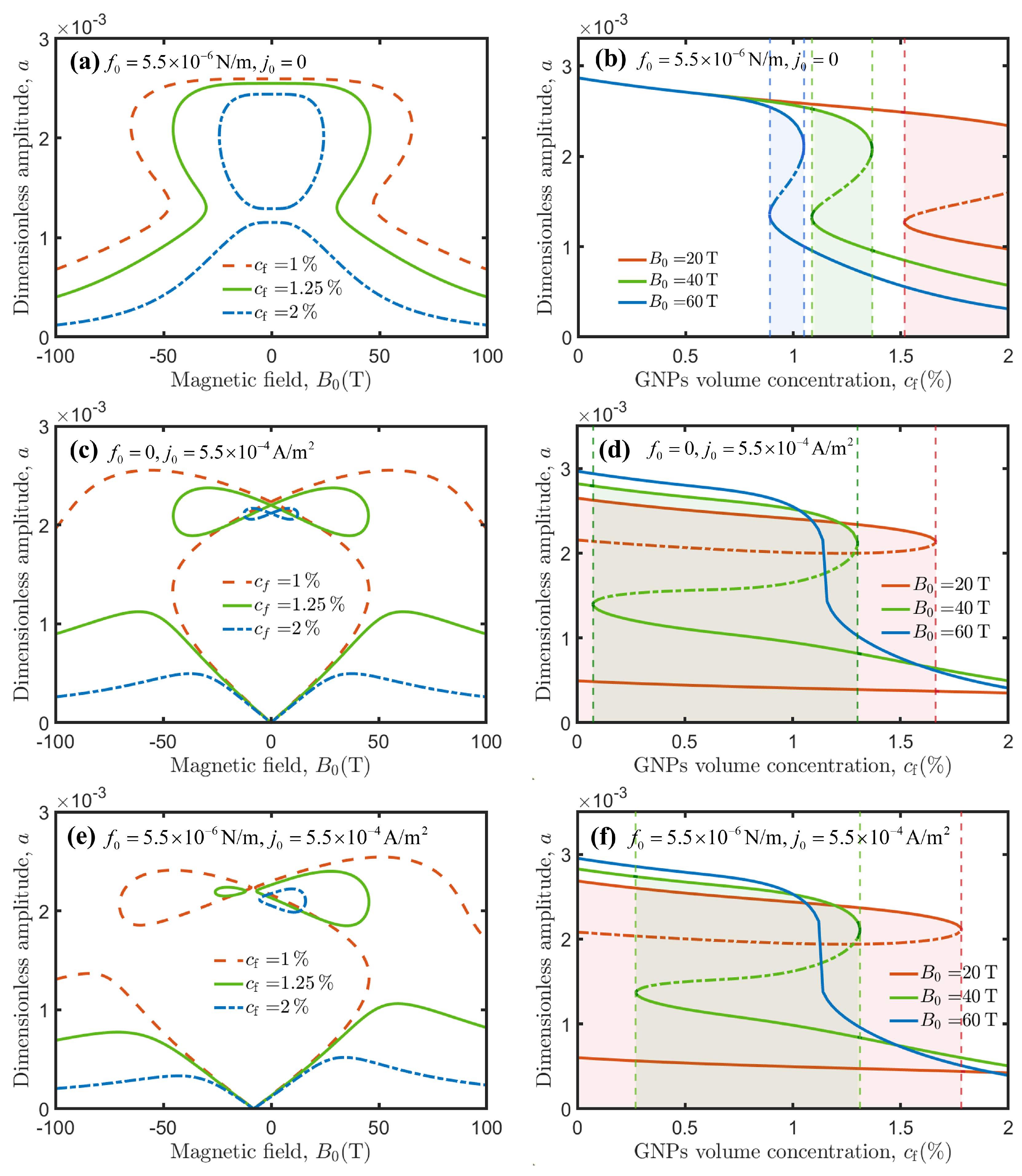
3.2.3. Amplitude-Magnetic Field Response

Figure 7 is the amplitude-magnetic field response diagrams and the corresponding amplitude-graphene concentration diagrams under different external loads, including LC1 [Figure 7a,b], LC2 [Figure 7c,d] and LC3 [Figure 7e,f]. In Figure 7a,c,e, there is an apparent negative value for the magnetic field, which means the magnetic field is opposite to the conventional direction. When subjected to only the external excitation force, the curves exhibit a left-right symmetric shape about the longitudinal axis B 0 = 0 , as shown in Figure 7a. As the external magnetic field strength reaches a certain value, the amplitude decreases significantly and the multi-valuedness of solutions disappears. As the concentration of graphene increases, the curve gradually symmetrically contracts into a ring shape with a slow decrease in amplitude. The critical separation point occurs at c f = 1.894%. When loaded only by the external current as shown in Figure 7b, the curve gradually and symmetrically shrinks into a double-node shape with increasing graphene volume concentration and the amplitude decreases slowly, and its critical separation point is c f = 1.148%. The symmetry of the curves is broken when both the external excitation force and the external current are applied simultaneously, as shown in Figure 7c. With the increase in graphene volume concentration, the amplitude curves showed the change rule of asymmetric inward contraction into a double-newline shape and the amplitude slowly decreasing. The curve on the negative magnetic field separates first, with a critical point of c f = 0.975%, and the critical separate point on the positive magnetic field is c f = 1.126%. When the concentration continues to rise to c f = 1.314%, the multi-value branch on the negative side disappears, and the amplitude decreases significantly.
In addition, the amplitude-graphene volume concentration curve [Figure 7b,d,f] demonstrates that the external magnetic field strength has a significant impact on the range of the system’s multi-valued region. As the strength of the magnetic field increases, the multi-valued region considerably narrows and may even vanish entirely, leading to a noticeable shift in its position toward the forward direction.
The nonlinear amplitude-magnetic field response in Figure 7 exhibits characteristic trends consistent with prior studies on magnetoelastic systems under ultrahigh fields [36]. While the absolute field magnitudes differ, the observed asymmetry in amplitude modulation and critical transitions aligns with reported nonlinear behaviors driven by Lorentz force dominance. This agreement validates the model’s capability to capture fundamental electromagnetic-elastic coupling mechanisms.

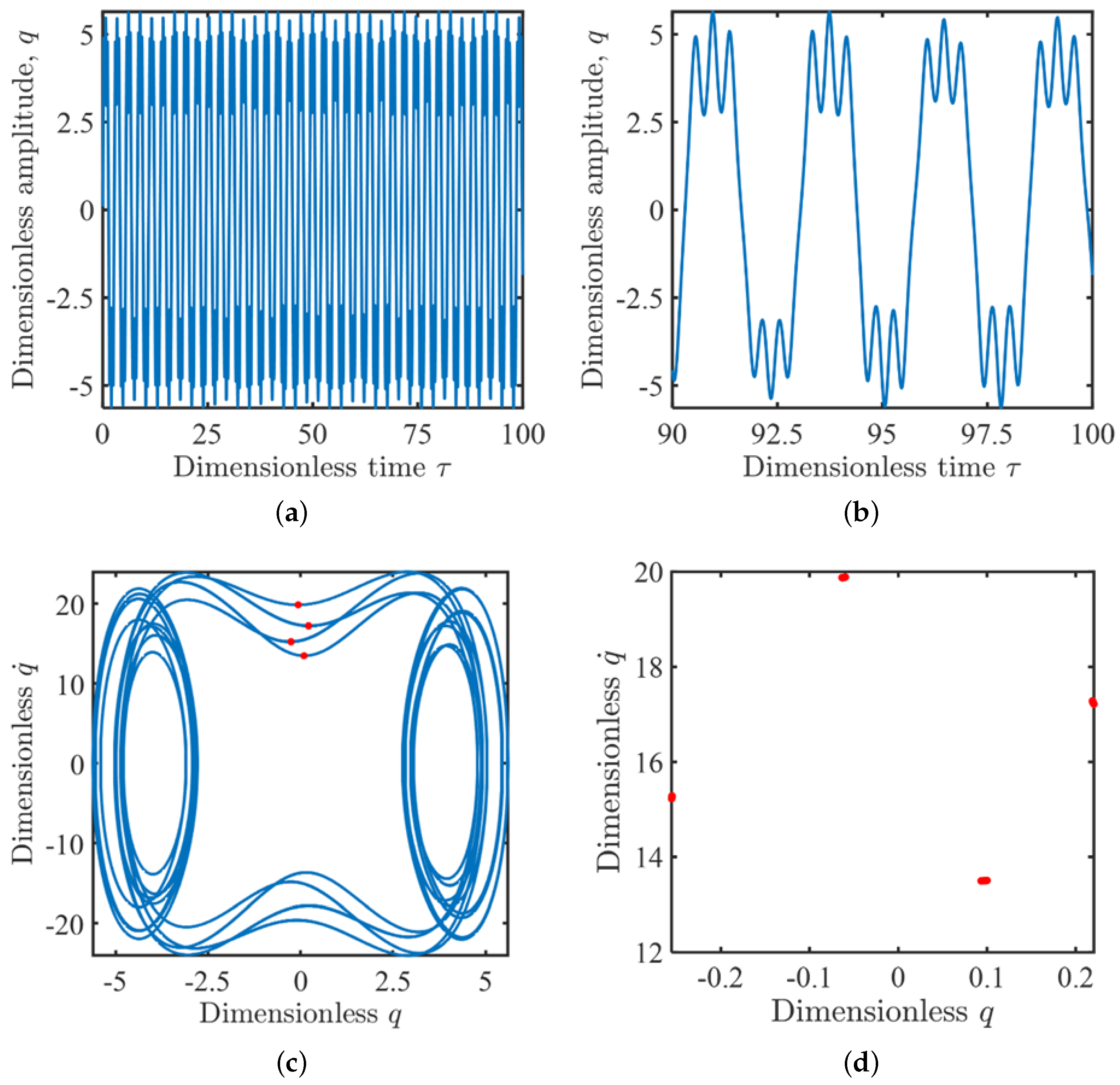
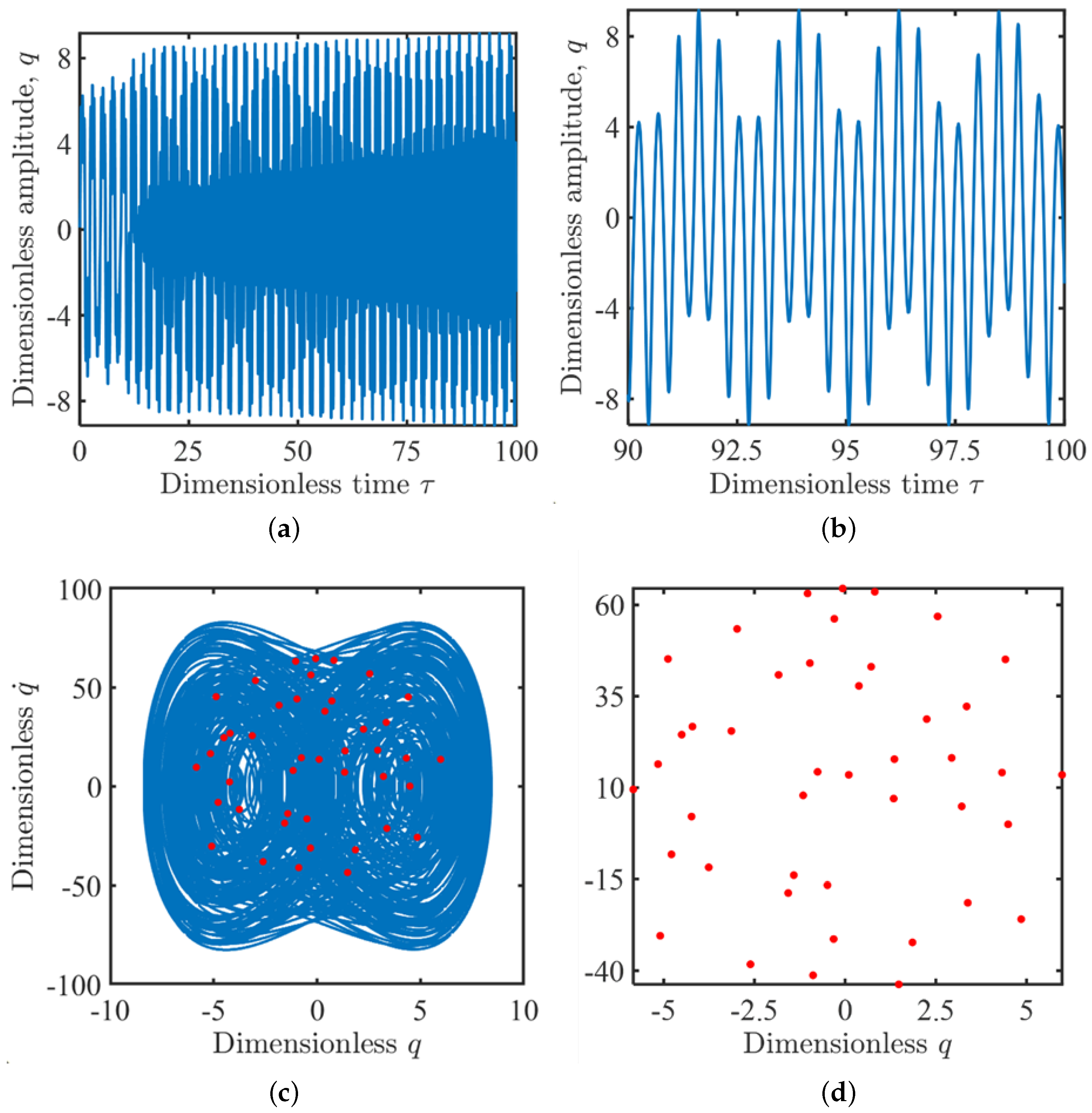
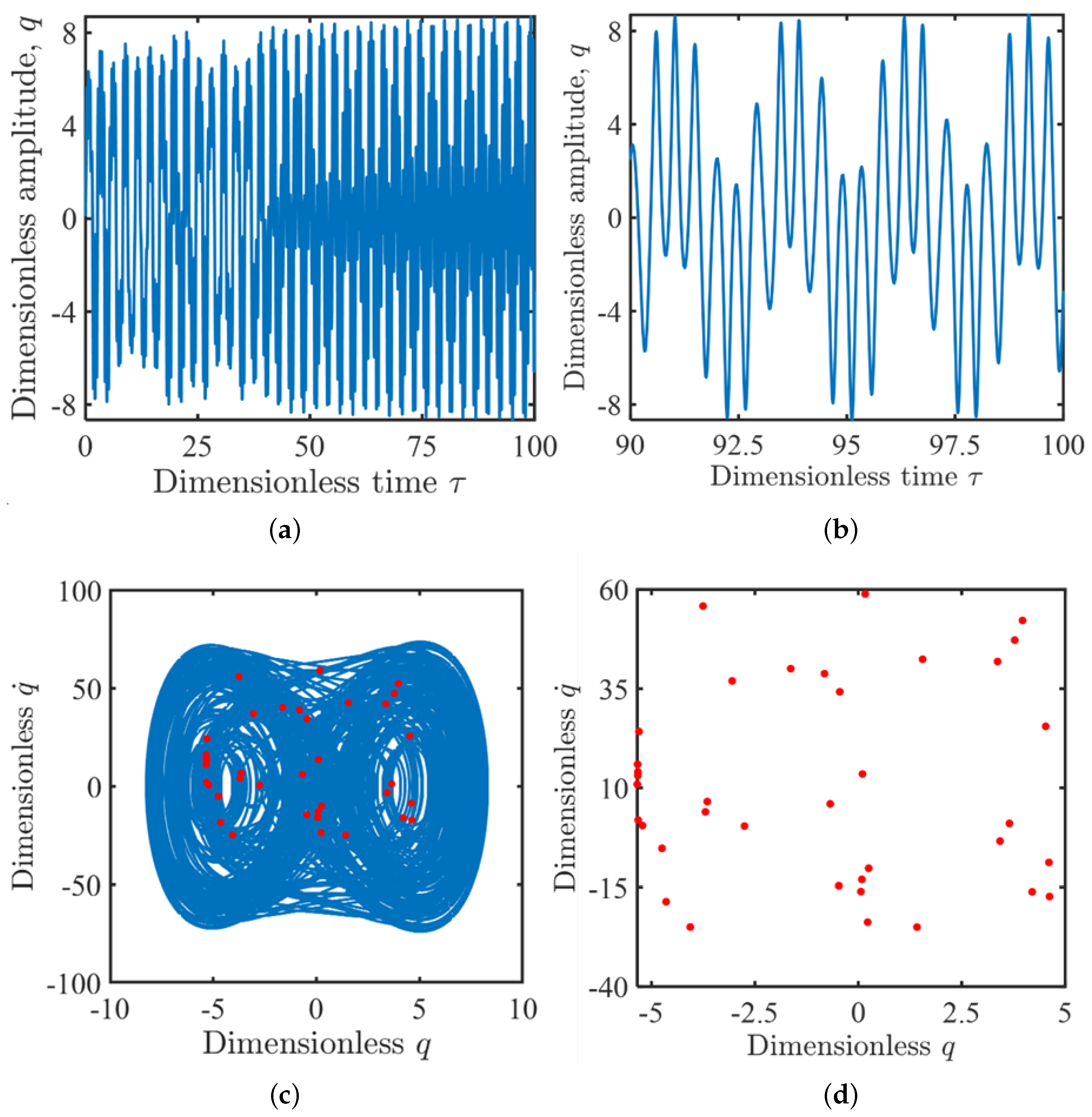
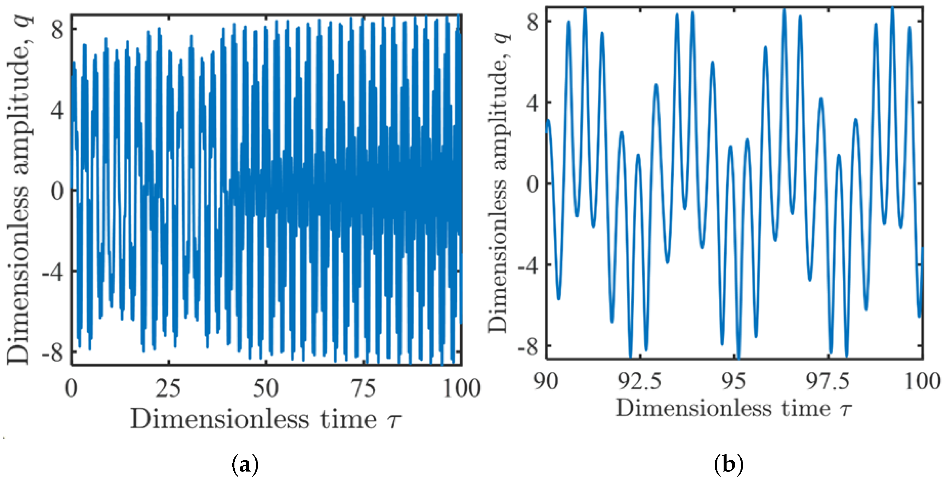
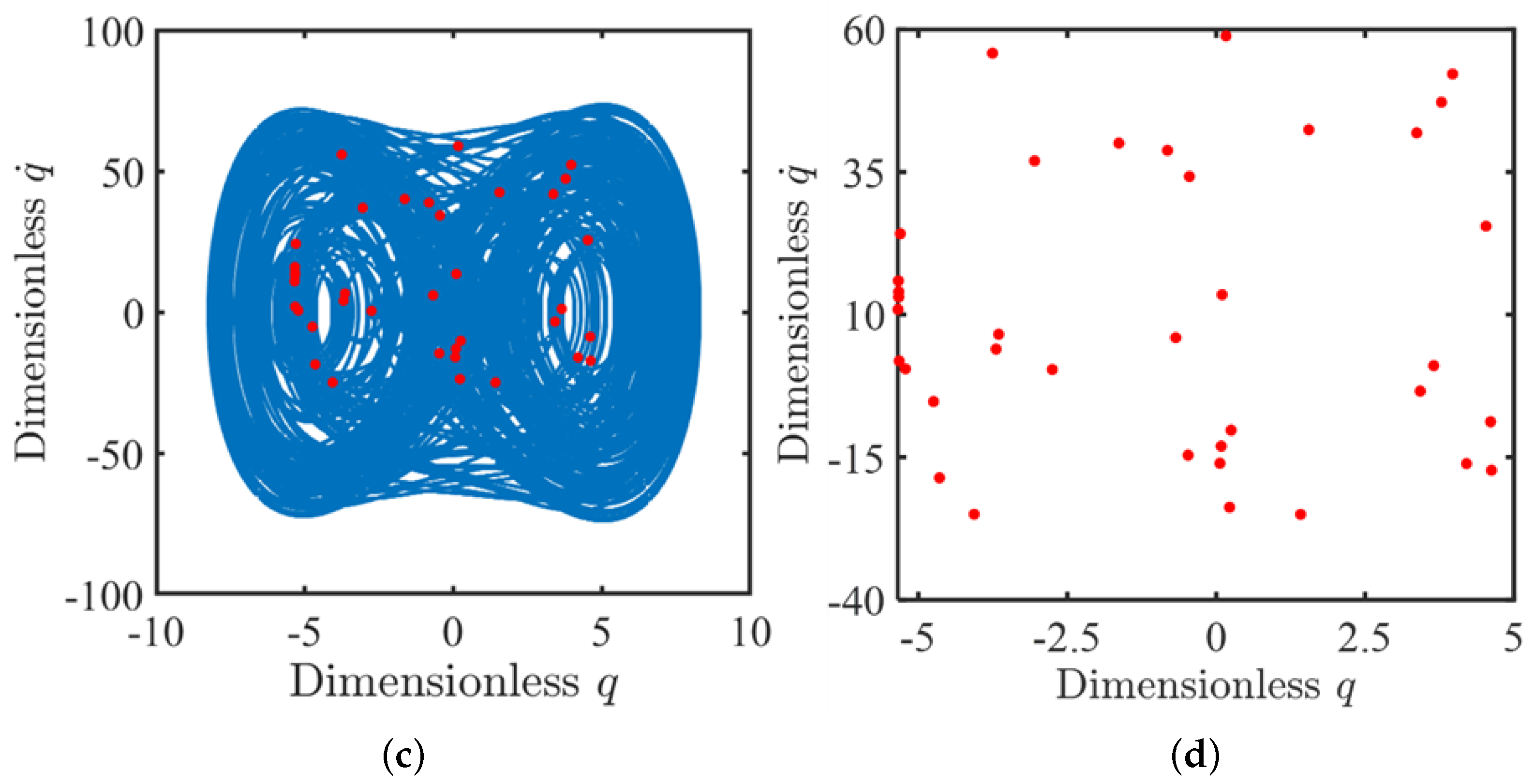
3.2.4. Period-Doubling and Chaotic Motion

The system vibration control Equation (9) is numerically solved for the ideal case of large external excitation (taking the external excitation force amplitude f 0 = 1.1 × 10 5 N/m, the applied magnetic field strength B 0 = 40 T, and the externally loaded current j 0 = 9 × 10 6 A / m 2 ). We set the initial value of the system q as 0.0033, q ˙ as 0.4502 and tune ε σ as -0.01. The time history diagram, waveform diagram, phase diagram, and Poincaré diagram of system transverse vibration are plotted in Figure 8. As for the red dots in Figure 8c, they are the same as those in Figure 8d,c is plotted simply by adding the Poincaré diagram to the phase diagram. The system does double periodic motion, and the phase diagram is relatively stable. Observing the time history diagram, the graph changes periodically, which is consistent with the period-doubling motion of the system.
Increasing the graphene filler concentration to 0.5% induces a transition from period-doubling to chaotic motion, as numerically demonstrated in Figure 9. The time history exhibits aperiodic oscillations with irregular amplitude modulation, while the phase portrait reveals a fractal-like trajectory structure, characteristic of deterministic chaos. The scattered Poincaré points, which lack periodic clustering, further confirm the loss of long-term stability. This behavior arises from the enhanced electrical conductivity of the nanocomposite at higher graphene loading, which amplifies nonlinear electromagnetic damping effects and destabilizes the harmonic balance.
By increasing the external excitation force to 2.1 × 10 5 N/m and numerically solving the system with the same initial conditions, it was observed that the system enters a state of chaotic motion as shown in Figure 10. When compared to the system under an external excitation force of 1.1 × 10 5 N/m, the phase portrait exhibits expanded trajectories with higher fractal dimensionality, indicating stronger nonlinear energy dissipation. Additionally, the Poincaré map displays a broader scattering of points, reflecting the dominance of inertial-electromagnetic coupling over damping stabilization. These features highlight how mechanical excitation amplitude critically modulates the transition depth and spectral complexity of chaos.
By reducing the external current to 9 × 10 5 A / m 2 and numerically solving the system with the same initial conditions, it was observed that the system entered a state of chaotic motion as shown in Figure 11. When compared to the system under an external load current of 9 × 10 6 A / m 2 , the phase portrait exhibits elongated trajectories with reduced curvature, indicating the dominance of inertial forces over electromagnetic constraints. Furthermore, the Poincaré map reveals asymmetric clustering of points, suggesting a shift in instability pathways driven by current-dependent nonlinear interactions. This contrast underscores the sensitivity of chaotic modes to electromagnetic excitation intensity.

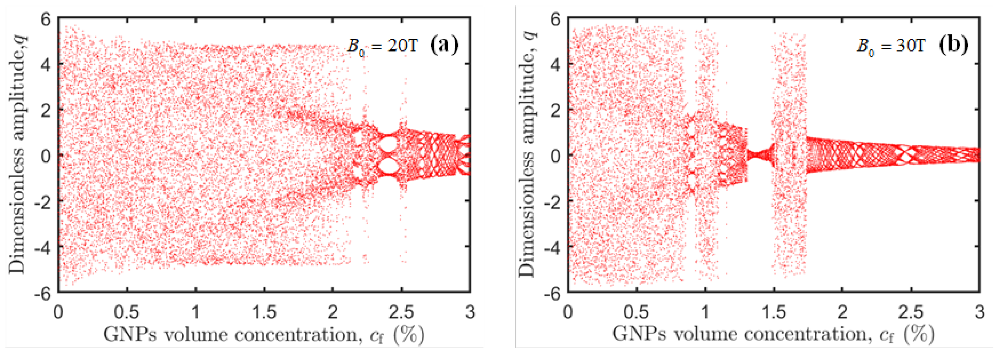
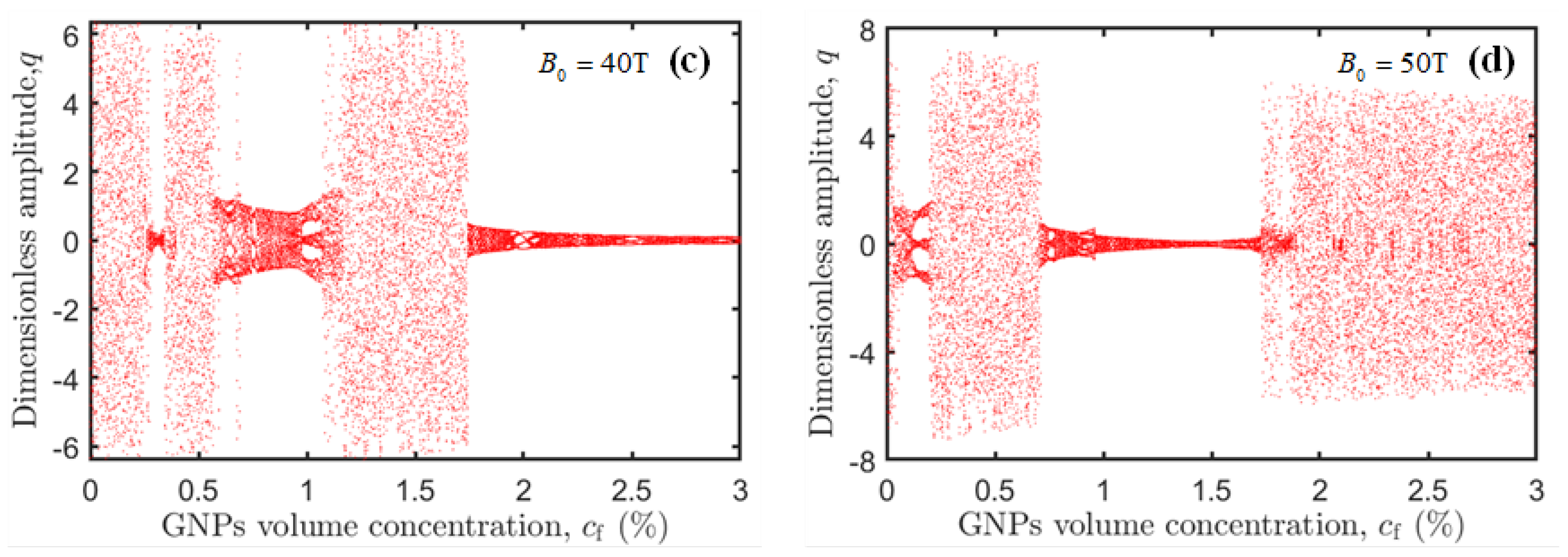
3.3. Bifurcation and Chaos Behaviors

Bifurcation and chaos are fundamental features of nonlinear dynamical systems, directly governing the long-term stability of deep-space components [41,42]. We furthermore investigate the influence of GNPs’ volume concentration to the system’s stability. Based on the parameters used in the previous section, and by varying the concentration of GNPs, we achieved the bifurcation diagram of the system.
Figure 12 is the system’s bifurcation diagram about GNPs’ volume concentration under different external magnetic field strengths, including Figure 12a for B 0 = 20 T, Figure 12b for B 0 = 30 T, Figure 12c for B 0 = 40 T, and Figure 12d B 0 = 50 T. From Figure 12b,c we can know that, as the GNPs’ volume concentration increases, the system’s bifurcation diagram generally experiences six stages. The system starts as a chaotic motion, and then turns to a periodic motion with a narrow range of volume concentration; then, it turns back to a chaotic motion and continues to change into a periodic motion with a wider range. The system will once again turn into a chaotic motion, and finally, the system will shift back to a periodic motion and stay that way.
As the external magnetic field strength increases from 20 T to 50 T, the system’s bifurcation diagrams, shown as Figure 12a–d, experienced some changes as well. With the rise in external magnetic field strength, the range of the first chaotic motion narrows, and the range of the second and the third chaotic motion area widens; also, the range of the first and the second periodic motion area widens, and the vibration amplitude of the third periodic motion decreases.

4. Conclusions

This study establishes a unified theoretical framework bridging micromechanics and nonlinear dynamics for graphene nanocomposites in extreme electromagnetic environments. By integrating effective medium theory with shear lag and Mori-Tanaka methods, the proposed model systematically addresses interfacial effects, agglomeration phenomena, and percolation thresholds. The model’s predictions align closely with experimental data, validating its capability to capture the coupled mechanical-electrical properties under multiphysics conditions.
Nonlinear dynamic analyses reveal that electromagnetic forces critically govern system stability, with graphene concentration and magnetic field strength jointly dictating transitions between periodic and chaotic regimes. Bifurcation studies demonstrate that a higher filler content amplifies nonlinear resonance amplitudes, while intensified magnetic fields suppress chaotic tendencies by modulating critical thresholds. Asymmetric amplitude-frequency responses under combined loads further emphasize the necessity of multiphysics coupling in design optimization.
Chaos analysis identifies distinct pathways through which material composition and external excitation drive dynamical instabilities. The fractal characteristics of phase diagrams and Poincaré maps highlight graphene’s dual role as a reinforcement agent and a nonlinearity modulator. These insights provide actionable strategies for tailoring graphene composites in aerospace applications, balancing structural performance with vibrational stability. Future work will extend this framework to time-dependent electromagnetic interactions and probabilistic agglomeration models, enhancing its predictive robustness.

Supplementary Materials

The following supporting information can be downloaded at: https://www.mdpi.com/article/10.3390/sym17050651/s1, Figure S1: Schematics for shear-lag theory.

Author Contributions

L.W.: Methodology, Software, Formal analysis, Writing, Visualization. J.W.: Conceptualization, Methodology, Formal analysis, Writing, Visualization, Funding acquisition. J.H.: Conceptualization, Methodology, Formal Analysis, Writing. X.P.: Methodology, Software. L.G.: Software, Formal analysis, Writing, Funding acquisition. All authors have read and agreed to the published version of the manuscript.

Funding

This work was supported by the National Nature Science Foundation of China (Grant No. 12302464 and No. 12202087), the Science and Technology Research Program of Chongqing Municipal Education Commission (Grant No. KJQN202300725).

Data Availability Statement

The codes developed are not public. However, the interested reader can contact the corresponding author to request the files.

Conflicts of Interest

The authors declare to have no conflict of interest.

References

  1. Kopperger, E.; List, J.; Madhira, S.; Rothfischer, F.; Lamb, D.C.; Simmel, F.C. A self-assembled nanoscale robotic arm controlled by electric fields. Science 2018, 359, 296–301. [Google Scholar] [CrossRef] [PubMed]
  2. Zhang, P.; Teng, Z.; Zhao, L.; Liu, Z.; Yu, X.; Zhu, X.; Peng, S.; Wang, T.; Qiu, J.; Wang, Q.; et al. Multi-Dimensional Mechanical Mapping Sensor Based on Flexoelectric-Like and Optical Signals. Adv. Sci. 2023, 10, 2301214. [Google Scholar] [CrossRef]
  3. Islam, M.H.; Afroj, S.; Uddin, M.A.; Andreeva, D.V.; Novoselov, K.S.; Karim, N. Graphene and CNT-based smart fiber-reinforced composites: A review. Adv. Funct. Mater. 2022, 32, 2205723. [Google Scholar] [CrossRef]
  4. Sun, X.; Huang, C.; Wang, L.; Liang, L.; Cheng, Y.; Fei, W.; Li, Y. Recent progress in graphene/polymer nanocomposites. Adv. Mater. 2021, 33, 2001105. [Google Scholar] [CrossRef]
  5. Lava Kumar, P.; Lombardi, A.; Byczynski, G.; Narayana Murty, S.V.S.; Murty, B.S.; Bichler, L. Recent advances in aluminium matrix composites reinforced with graphene-based nanomaterial: A critical review. Prog. Mater. Sci. 2022, 128, 100948. [Google Scholar] [CrossRef]
  6. Meng, Q.; Araby, S.; Oh, J.A.; Chand, A.; Zhang, X.; Kenelak, V.; Ma, J.; Liu, T.; Ma, J. Accurate self-damage detection by electrically conductive epoxy/graphene nanocomposite film. J. Appl. Polym. Sci. 2021, 138, 50452. [Google Scholar] [CrossRef]
  7. Xia, X.; Hao, J.; Wang, Y.; Zhong, Z.; Weng, G.J. Theory of electrical conductivity and dielectric permittivity of highly aligned graphene-based nanocomposites. J. Phys. Condens. Matter 2017, 29, 205702. [Google Scholar] [CrossRef] [PubMed]
  8. Papageorgiou, D.G.; Kinloch, I.A.; Young, R.J. Mechanical properties of graphene and graphene-based nanocomposites. Prog. Mater. Sci. 2017, 90, 75–127. [Google Scholar] [CrossRef]
  9. Young, R.J.; Liu, M.; Kinloch, I.A.; Li, S.; Zhao, X.; Vallés, C.; Papageorgiou, D.G. The mechanics of reinforcement of polymers by graphene nanoplatelets. Compos. Sci. Technol. 2018, 154, 110–116. [Google Scholar] [CrossRef]
  10. Papageorgiou, D.G.; Li, Z.; Liu, M.; Kinloch, I.A.; Young, R.J. Mechanisms of mechanical reinforcement by graphene and carbon nanotubes in polymer nanocomposites. Nanoscale 2020, 12, 2228–2267. [Google Scholar] [CrossRef]
  11. Ebrahimi, F.; Dabbagh, A. Vibration analysis of multi-scale hybrid nanocomposite plates based on a Halpin-Tsai homogenization model. Compos. Part B Eng. 2019, 173, 106955. [Google Scholar] [CrossRef]
  12. Zhao, T.Y.; Cui, Y.S.; Pan, H.G.; Yuan, H.Q.; Yang, J. Free vibration analysis of a functionally graded graphene nanoplatelet reinforced disk-shaft assembly with whirl motion. Int. J. Mech. Sci. 2021, 197, 106335. [Google Scholar] [CrossRef]
  13. Weng, G.J. Some elastic properties of reinforced solids, with special reference to isotropic ones containing spherical inclusions. Int. J. Eng. Sci. 1984, 22, 845–856. [Google Scholar] [CrossRef]
  14. Sadeghpour, E.; Guo, Y.; Chua, D.; Shim, V.P.W. A modified Mori–Tanaka approach incorporating filler-matrix interface failure to model graphene/polymer nanocomposites. Int. J. Mech. Sci. 2020, 180, 105699. [Google Scholar] [CrossRef]
  15. Fedotov, A.F. Mori-Tanaka experimental-analytical model for predicting engineering elastic moduli of composite materials. Compos. Part B Eng. 2022, 232, 109635. [Google Scholar] [CrossRef]
  16. Weng, G.J. The theoretical connection between Mori-Tanaka’s theory and the Hashin-Shtrikman-Walpole bounds. Int. J. Eng. Sci. 1990, 28, 1111–1120. [Google Scholar] [CrossRef]
  17. Huang, Y.; Hu, K.X.; Chandra, A. Several variations of the generalized self-consistent method for hybrid composites. Compos. Sci. Technol. 1994, 52, 19–27. [Google Scholar] [CrossRef]
  18. Weng, G.J. A dynamical theory for the Mori–Tanaka and Ponte Castañeda–Willis estimates. Mech. Mater. 2010, 42, 886–893. [Google Scholar] [CrossRef]
  19. Nan, C.W.; Birringer, R.; Clarke, D.R.; Gleiter, H. Effective thermal conductivity of particulate composites with interfacial thermal resistance. J. Appl. Phys. 1997, 81, 6692–6699. [Google Scholar] [CrossRef]
  20. Su, Y.; Li, J.J.; Weng, G.J. Theory of thermal conductivity of graphene-polymer nanocomposites with interfacial Kapitza resistance and graphene-graphene contact resistance. Carbon 2018, 137, 222–233. [Google Scholar] [CrossRef]
  21. Wang, Y.; Feng, C.; Wang, X.; Zhao, Z.; Romero, C.S.; Yang, J. Nonlinear free vibration of graphene platelets (GPLs)/polymer dielectric beam. Smart Mater. Struct. 2019, 28, 055013. [Google Scholar] [CrossRef]
  22. Li, X.; Song, M.; Yang, J.; Kitipornchai, S. Primary and secondary resonances of functionally graded graphene platelet-reinforced nanocomposite beams. Nonlinear Dyn. 2019, 95, 1807–1826. [Google Scholar] [CrossRef]
  23. Gholami, R.; Ansari, R. Nonlinear harmonically excited vibration of third-order shear deformable functionally graded graphene platelet-reinforced composite rectangular plates. Eng. Struct. 2018, 156, 197–209. [Google Scholar] [CrossRef]
  24. Song, M.; Gong, Y.; Yang, J.; Zhu, W.; Kitipornchai, S. Free vibration and buckling analyses of edge-cracked functionally graded multilayer graphene nanoplatelet-reinforced composite beams resting on an elastic foundation. J. Sound Vib. 2019, 458, 89–108. [Google Scholar] [CrossRef]
  25. Song, M.; Gong, Y.; Yang, J.; Zhu, W.; Kitipornchai, S. Nonlinear free vibration of cracked functionally graded graphene platelet-reinforced nanocomposite beams in thermal environments. J. Sound Vib. 2020, 468, 115115. [Google Scholar] [CrossRef]
  26. Wei, D.; Nurakhmetov, D.; Aniyarov, A.; Zhang, D.; Spitas, C. Lumped-parameter model for dynamic monolayer graphene sheets. J. Sound Vib. 2022, 534, 117062. [Google Scholar] [CrossRef]
  27. Vila, J.; Fernández-Sáez, J.; Zaera, R. Reproducing the nonlinear dynamic behavior of a structured beam with a generalized continuum model. J. Sound Vib. 2018, 420, 296–314. [Google Scholar] [CrossRef]
  28. Jalaei, M.H.; Thai, H.T.; Civaek, Ö. On viscoelastic transient response of magnetically imperfect functionally graded nanobeams. Int. J. Eng. Sci. 2022, 172, 103629. [Google Scholar] [CrossRef]
  29. Eshelby, J.D. The determination of the elastic field of an ellipsoidal inclusion, and related problems. Proc. R. Soc. London. Ser. A. Math. Phys. Sci. 1957, 241, 376–396. [Google Scholar]
  30. Wang, J.; Li, J.J.; Weng, G.J.; Su, Y. The effects of temperature and alignment state of nanofillers on the thermal conductivity of both metal and nonmetal based graphene nanocomposites. Acta Mater. 2020, 185, 461–473. [Google Scholar] [CrossRef]
  31. Wang, J.; Li, C.; Li, J.; Weng, G.J.; Su, Y. A multiscale study of the filler-size and temperature dependence of the thermal conductivity of graphene-polymer nanocomposites. Carbon 2021, 175, 259–270. [Google Scholar] [CrossRef]
  32. Gong, L.; Kinloch, I.A.; Young, R.J.; Riaz, I.; Jalil, R.; Novoselov, K.S. Interfacial stress transfer in a graphene monolayer nanocomposite. arXiv 2010, arXiv:1007.1953. [Google Scholar] [CrossRef]
  33. Wang, J.; Gong, L.; Xi, S.; Li, C.; Su, Y.; Yang, L. Synergistic effect of interface and agglomeration on Young’s modulus of graphene-polymer nanocomposites. Int. J. Solids Struct. 2024, 292, 112716. [Google Scholar] [CrossRef]
  34. Li, C.; Wang, J.; Su, Y. A dual-role theory of the aspect ratio of the nanofillers for the thermal conductivity of graphene-polymer nanocomposites. Int. J. Eng. Sci. 2021, 160, 103453. [Google Scholar] [CrossRef]
  35. Wang, Y.; Weng, G.J.; Meguid, S.A.; Hamouda, A.M. A continuum model with a percolation threshold and tunneling-assisted interfacial conductivity for carbon nanotube-based nanocomposites. J. Appl. Phys. 2014, 115, 193706. [Google Scholar] [CrossRef]
  36. Wang, L.; Wang, J.; Zhang, M.; Gong, L. Magneto-elastic vibration of axially moving graphene nanocomposite current-carrying beam with variable speed and axial force. Acta Mech. 2024, 235, 5747–5763. [Google Scholar] [CrossRef]
  37. Hu, Y.; Wang, J. Principal-internal resonance of an axially moving current-carrying beam in magnetic field. Nonlinear Dyn. 2017, 90, 683–695. [Google Scholar] [CrossRef]
  38. Beskin, V.S.; Balogh, A.; Falanga, M.; Treumann, R.A. Magnetic Fields at Largest Universal Strengths: Overview. Space Sci. Rev. 2015, 191, 1–12. [Google Scholar] [CrossRef]
  39. Hahn, S.; Kim, K.; Kim, K.; Hu, X.; Painter, T.; Dixon, I.; Kim, S.; Bhattarai, K.R.; Noguchi, S.; Jaroszynski, J.; et al. 45.5-tesla direct-current magnetic field generated with a high-temperature superconducting magnet. Nature 2019, 570, 496–499. [Google Scholar] [CrossRef]
  40. Ji, J.C.; Zhang, N. Suppression of the primary resonance vibrations of a forced nonlinear system using a dynamic vibration absorber. J. Sound Vib. 2010, 329, 2044–2056. [Google Scholar] [CrossRef]
  41. Chen, G.; Moiola, J.L. An overview of bifurcation, chaos and nonlinear dynamics in control systems. J. Frankl. Inst. 1994, 331, 819–858. [Google Scholar] [CrossRef]
  42. Luo, A.C.J. Bifurcation and Stability in Nonlinear Dynamical Systems; Springer: Cham, Switzerland, 2019. [Google Scholar]
Figure 1. The comparison of calculated effective Young’s modulus and electrical conductivity of GNP-epoxy composites with experimental data by Meng et al. [6] and Xia et al. [7].
Symmetry 17 00651 g001
Figure 2. The current-carrying nanocomposite beam undergoing axial translation in magnetic field.
Symmetry 17 00651 g002
Figure 3. The comparison of the dynamic response curve of the system using three different model assumptions: MA1 (blue dash-dot line), MA2 (green solid line), and MA3 (orange dash line). (a) magnetic field-axial velocity singularity distribution; (b) axial force-velocity singularity distribution, respectively; (c) first-order principal amplitude-frequency curves of the model under only external force; (d) first-order principal amplitude-frequency curves of the model under combined external force and external current.
Symmetry 17 00651 g003
Figure 4. The stable singularity distribution of (a) magnetic field vs. axial velocity and (b) magnetic field vs. graphene volume concentration.
Symmetry 17 00651 g004
Figure 5. The primary resonance response of an axially moving current-loaded nanocomposite beam under different external loads, including (a,b), under external excitation force; (c,d), under external current; (e,f), under both external force and external current; (a,c,e), amplitude-frequency responses, (b,d,f), amplitude-graphene volume concentration curves.
Symmetry 17 00651 g005aSymmetry 17 00651 g005b
Figure 6. The primary resonance response of an axially moving current-loaded nanocomposite beam under different external loads, including (a,b) the external excitation force (LC1); (c,d) the external current (LC2); (e,f) both external force and the external current (LC3). (a,c) Amplitude-external load response curves and (b,d) orresponding amplitude-graphene volume concentration curves. (f) Top view of (e) the 3D primary resonance diagrams.
Symmetry 17 00651 g006aSymmetry 17 00651 g006b
Figure 7. The primary resonance response of an axially moving current-loaded nanocomposite beam under different external loads, including (a,b) for LC1; (c,d) the external current for LC2; (e,f) for LC3. (a,c,e) Amplitude-magnetic field response curves, and (b,d,f) the corresponding amplitude-graphene volume concentration curves.
Symmetry 17 00651 g007
Figure 8. Period-doubling response of the system. (a) time history diagram; (b) waveform diagram; (c) phase diagram; (d) Poincaré diagram.
Symmetry 17 00651 g008
Figure 9. The chaotic response of the system (0.5% graphene filler). (a) time history diagram; (b) waveform diagram; (c) phase diagram; (d) Poincaré diagram.
Symmetry 17 00651 g009
Figure 10. The chaotic response of the system ( f 0 = 1.1 × 10 5 N/m). (a) time history diagram; (b) waveform diagram; (c) phase diagram; (d) Poincaré diagram.
Symmetry 17 00651 g010
Figure 11. The chaotic response of the system ( j 0 = 9 × 10 5 A / m 2 ). (a) time history diagram; (b) waveform diagram; (c) phase diagram; (d) Poincaré diagram.
Symmetry 17 00651 g011aSymmetry 17 00651 g011b
Figure 12. The system’s bifurcation diagram about GNPs’ volume concentration under different external magnetic field strength, including (a) for B 0 = 20 T; (b) for B 0 = 30 T; (c) for B 0 = 40 T; (d) B 0 = 50 T.
Symmetry 17 00651 g012aSymmetry 17 00651 g012b
Disclaimer/Publisher’s Note: The statements, opinions and data contained in all publications are solely those of the individual author(s) and contributor(s) and not of MDPI and/or the editor(s). MDPI and/or the editor(s) disclaim responsibility for any injury to people or property resulting from any ideas, methods, instructions or products referred to in the content.

