Advancing Decision-Making in AI Through Bayesian Inference and Probabilistic Graphical Models

Abstract

The navigation of autonomous vehicles should be accurate and reliable to navigate safely in changing and unpredictable conditions. This paper proposes an advanced autonomous vehicle navigation framework that integrates probabilistic graphical models, Markov Chain Monte Carlo methods, and Bayesian optimization to enable reliable, real-time decision-making in uncertain environments. Due to dynamic and unpredictable surroundings, autonomous navigation is highly challenged in uncertainty quantification and adaptive parameter tuning. By leveraging PGMs, the framework can first determine probabilistic dependencies between critical variables, i.e., nodes and edges, such as vehicle speed, obstacle proximity, and environmental factors, to create a robust foundation for situational awareness. Then, Bayesian inference is obtained using MCMC: the system updates its real-time beliefs as new sensor data become available. The inference layer allows adaptation to unexpected obstacles by revising trajectories or controlling a vehicle’s speed while improving safety and reliability. Finally, Bayesian optimization fine-tunes key parameters within the system, such as sensor thresholds and control variables, maximizing efficiency without exhaustive manual tuning of these parameters. Using a multi-sensor data source with images, LiDAR, radar, and annotated environmental features, the Lyft Level 5 Perception Dataset tested real-world navigation scenarios against the framework. This proposed framework’s accuracy was around 99.01% and signified good decision-making capabilities for an autonomous vehicle navigating through complex environments with reliable performance. The autonomous vehicle system is also intended to provide improved safety and flexibility in complex environments, promising the development of more resilient and dependable AI-driven solutions for navigation.

1. Introduction

The development of autonomous navigation has a rich history that dates back to the 20th century, when leading research began for the building blocks that shaped the advancements of the modern day. One of the earliest, highly notable projects was the Stanford Cart, developed in the 1980s, demonstrating feasibility in robotic navigation through a controlled environment by passing successfully through obstacles using simple sensors. Over the years, sensor technologies have advanced. LiDAR and cameras with high resolutions greatly enhanced vehicles’ ability to perceive their surroundings. This was important because it made the development of advanced algorithms capable of interpreting complex sensory data for real-time decision-making possible [1]. Autonomous navigation has more important implications than mere convenience. It will likely ensure greater public safety and fewer traffic accidents and provide more accessibility for people who cannot drive [2]. This implies that, with the speedy development of smart cities and the IoT, the seamless integration of any autonomous vehicle into any present-day urban infrastructure will eventually be more critical than any other transportation system in the future [3,4]. These trends require novel algorithms that can execute the real-time processing of volumes of data and make judicious decisions in dynamic, unpredictable environments. Hence, some AI-based ML and DL approaches have been developed to surpass the challenges above to boost the navigation capabilities of autonomous systems [5,6,7].

To make the navigation of autonomous vehicles more robust, researchers have attempted to use several machine learning (ML), artificial intelligence (AI), and deep learning (DL) techniques, with their respective strengths and weaknesses, in the problem of navigation [8]. Traditional ML methods, such as decision trees and support vector machines, have been very widely used in tasks such as obstacle detection and path planning, thereby providing a basic foundation for initial navigation strategies [9]. With the advancement of technology, AI algorithms have become more dominant in optimizing routing strategies with real-time inputs to help vehicles adapt to changing traffic conditions. Meanwhile, DL methods, especially CNNs, have emerged as powerful tools for processing visual data, which is crucial for things like object recognition and scene understanding [10]. Additional time-series predictions need more recurrent neural networks and LSTM networks, which are more specific for forecasting behaviors in dynamic environments. Even though some methods may be able to complete thousands of predictions, they face hurdles in quantifying uncertainty while requiring large sets of labeled data, which demands vast periods of gathering of the sample needed for labeling the same data [11]. In addition, traditional hyperparameter tuning through grid search optimization may lead to inefficient space exploration of the parameters, with suboptimal model performance [12]. As such, there has been a growing need for hybrid approaches that bring out the best of traditional ML and DL approaches to address some of the complex issues found in autonomous navigation systems [13].

The proposed framework aims to overcome shortcomings in the previous ML, AI, and DL approaches applied to autonomous navigation. Traditional models may perform well in controlled or predictable environments but are not usually robust in complex, real-world scenarios characterized by dynamic changes and uncertainties [2]. Utilizing Bayesian inference and probabilistic graphical models, the approach constructs a better quantification of uncertainty capabilities in the system and results in more informed, robust real-time decisions over incoming data streams [14]. Besides these benefits, the introduction of Bayesian optimization presents an inherently formalized way to manage this crucial process, with the selection of hyperparameters for most ML problems, which usually consumes heavy resources and requires long computational periods [12]. This ability is critical for applications where quick and accurate responses can make all the difference in safety and operational efficiency. Finally, the proposed framework tries to establish a resilient navigation system that improves the accuracy of decision-making processes and enhances the adaptability of autonomous vehicles to the complexities of the real world. This tackles the pressing issues the current systems face, outlining a way toward more trustworthy and intelligent navigation solutions within the autonomous vehicle domain. The primary key contributions of this proposed framework are as follows:

• The proposed framework integrates probabilistic graphical models (PGMs), Markov Chain Monte Carlo (MCMC) methods, and Bayesian optimization to enhance visual target tracking for autonomous vehicles.
• It utilizes the Lyft Level 5 Perception Dataset for training and validating algorithms with diverse and high-quality sensor data.
• PGMs enable structured representations of relationships among environmental factors, improving situational awareness by capturing dependencies and uncertainties.
• MCMC methods facilitate real-time updates of the vehicle’s beliefs about its surroundings, dynamically adjusting tracking accuracy to changing conditions.
• Bayesian optimization optimizes system parameter tuning and sensor fusion, minimizing computational costs while ensuring effective adaptation to various operational scenarios.

The rest of this paper is divided into the following sections: Section 2 discusses related works on autonomous vehicle navigation systems and the application of deep learning techniques. Section 3 outlines the data for the proposed method. Section 4 gives the experimental results and discussion. Finally, Section 5 gives the conclusion.

2. Related Works

Mohammed [15] stated that using AI in the navigation of autonomous vehicles brings some advancements and issues. The focus of this paper is the evaluation of the AI algorithm that helps sensor fusion, which ensures effective perception of the environment and emphasizes aspects of transparency and trust, with tremendous potential for precision and safety for vehicles in their navigation. However, this research study discovered critical issues related to model explainability and cybersecurity that could be obstacles to the safe application in practical conditions of such technology.

Basu [16] shifted the attention from a control-based, old architecture to a more applicable ML model-based navigation system for autonomous vehicles. The report stated that the latest advances observed were in object detection, semantic mapping, and optimal path execution due to progress in machine learning technology. It also required standardized datasets and benchmarking environments to support further research. Nevertheless, the paper criticized the fact that existing models have yet to be developed for more robust safety mechanisms and human-like interpretability, which would be required for widespread deployment in dynamic environments.

Baliyan et al. [17] focused on integrating artificial intelligence and the Internet of Things (IoT) to develop improved technology for autonomous vehicles. They discussed how AI can reduce human error in driving, which is the cause of the majority of vehicular accidents, while promoting the safe operation of autonomous vehicles. They found that this would necessitate fully integrated sensing systems that feed real-time decision-making in AVs. This said, the authors noted that it remains a challenge to ensure a significantly lower acceptable risk threshold for AVs.

Ibrahim et al. [18] investigated some control techniques ensuring safe and efficient traversal in an autonomous vehicle within the environment. The work focused on the applicability of neuro-fuzzy systems with Particle Swarm Optimization to fine-tune and utilize CNNs and optimize them using the Adam algorithm. This facilitated decision-making in real-time based on an awareness of the surroundings due to the presence of the objects. However, the study indicated that despite reaching a high level of performance, the CNNs were relatively heavy and used more computing power compared to less complex models. This makes it challenging to implement such applications in resource-poor settings.

Prabhod [19] proposed a new framework based on reinforcement learning and deep learning techniques. This framework leveraged the capability of a large language model (LLM) for better real-time decision-making in dynamic environments. The results suggested that high-fidelity simulations create tremendous safety gains and compliance with traffic laws. However, the data-intensive usage of data in the training of RL agents could add limitations to the practical usage of the framework, especially when a scarcity of data exists.

Do et al. [20] demonstrated a prototype of an autonomous vehicle based on mono-vision using deep neural networks implemented on a Raspberry Pi device. The authors of the paper indicated a transition toward full autonomy from fully autonomous driving capabilities and CNNs applied by mapping raw input images onto steering angles to successfully guide the vehicle. In conclusion, the prototype was shown to be able to maintain a stable lane in diverse conditions, but its ability was limited by dependence on a small set of manual examples of how the roads and traffic could vary.

Critical Observation: The articles discussed contribute significantly to the discipline of autonomous vehicle navigation while employing AI, ML, and DL techniques. Some related studies suffer from a common limitation: model explainability and, more importantly, having safety mechanisms when models like CNNs are used. Such models have a high intensity of computations, which may be difficult to scale in any real-time application. While some research presented innovative approaches toward real-time decision-making, a big dataset requirement argues against their use in real-world applications when the situations are diverse and dynamic. On the other hand, implementations in real systems reveal many risks in trying to generalize learned or derived solutions to a greater number of scenarios where there may be less data. Thus, filling these gaps in the suggested framework will give more reliability and safety to the application of autonomous navigation systems.

3. Problem Statement

The increasing complexity and demand for autonomous vehicle navigation emphasize the need for advanced methodologies in robust visual target tracking. A review of the last decade indicates that although some significant advancements have been achieved, challenges persist, including the necessity for reliable algorithms adapted to varying environmental conditions and the effective integration of data from multiple sources. Traditional vision-based methods [21] are not robust in dynamic environments. Lighting changes and object occlusion degrade the overall performance. Moreover, although data fusion seems promising for enhanced tracking accuracy, it is computationally expensive and rather difficult to implement. To overcome these problems, the proposed framework integrates PGMs, MCMC methods, and Bayesian optimization. Such an approach introduces probabilistic dependencies of key variables for better environment representation and situational awareness. MCMC, for instance, enables adaptivity by real-time updates for changing sensor data, while Bayesian optimization streamlines parameter adaptation, ensuring efficient sensor data fusion and control adaptation that enhances the robustness of visual tracking in diverse settings.

4. Proposed Methodology: Probabilistic Graphical Models for Advanced Decision-Making in AI Through Bayesian Inference

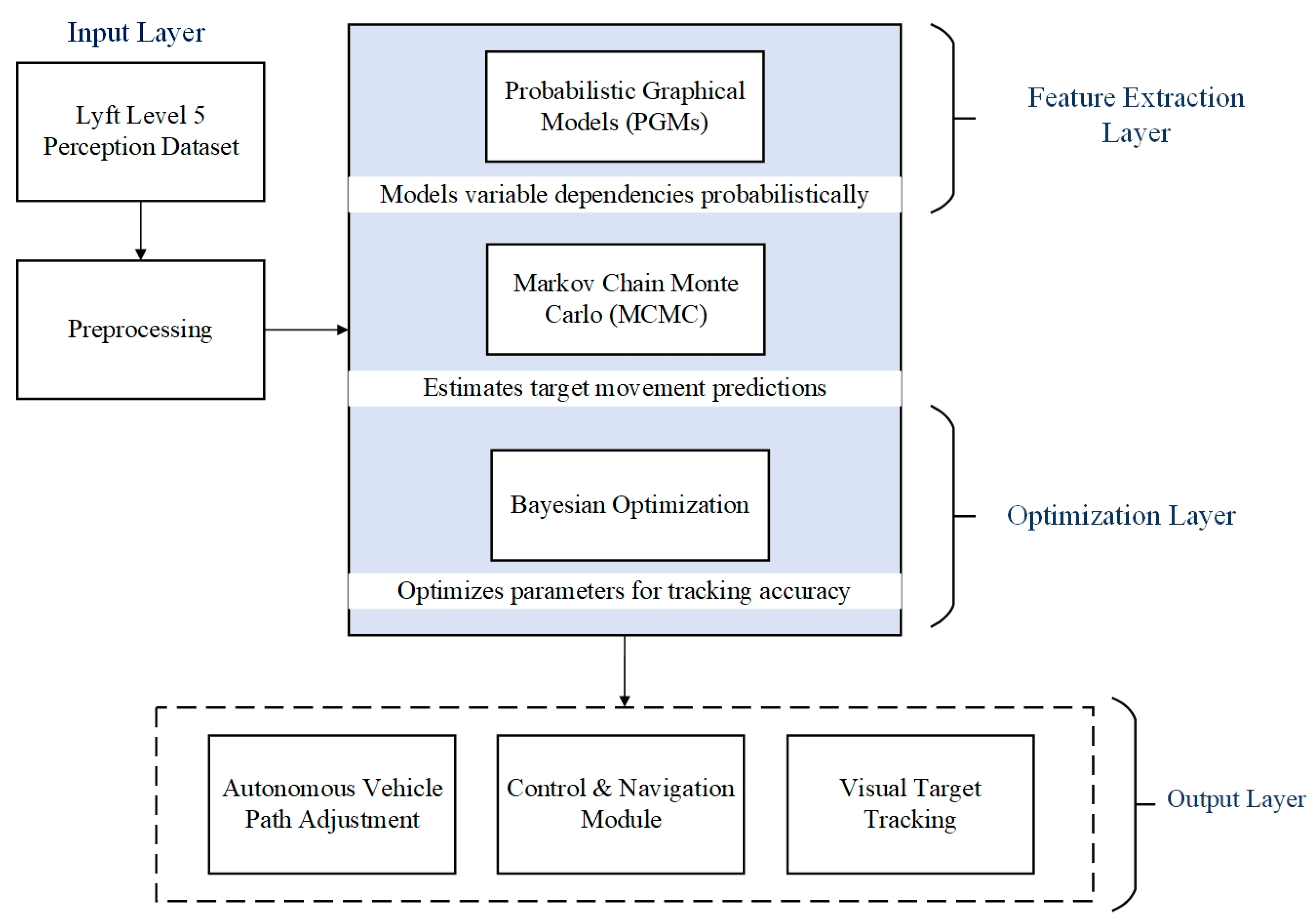
The proposed autonomous vehicle navigation framework dataset is a comprehensive collection of data from various sensors, such as LiDAR, camera, and radar, which are used to train and validate visual tracking and navigation algorithms on an autonomous vehicle. This dataset is processed by filtering, normalizing readings, aligning frames, and extracting relevant features. Relationships amongst observed variables and latent factors are established using probabilistic models called PGMS. Such models increase situational awareness and enable one to infer the possibilities of interactions a vehicle would have with its surroundings. Bayesian inference has MCMC-based algorithms for online updates regarding beliefs about a car’s environment. This approach allows for the real-time updating of predictions as it creates samples based on the probabilistic distributions established by the PGMs, and this accommodates the uncertainty and variations of the unpredictable motion of a vehicle on a path, as shown in Figure 1.

Bayesian optimization is carried out for adjustments in model parameters, with the fine-tuning procedures within sensor fusion; this ensures that good tracking systems are provided with minimum stress on the cost of computations. With this information, visual object tracking is possible in the operational range of the vehicle. The data are utilized to find appropriate paths and actions for the vehicle. The control module interprets tracking data using input from the visual tracking system and decision-making algorithms for the most appropriate path for the vehicle. The vehicle’s path is constantly updated to avoid obstacles along its trajectory and keep the trajectory of the vehicle safe. The autonomous vehicle’s target tracking algorithm, advanced probabilistic methods, and real-time optimization and control mechanisms ensure resilient adaptability.

4.1. Dataset Description

The Lyft Level 5 Perception Dataset is a rich, multi-sensor autonomous vehicle research and development dataset. It captures various driving scenarios and environments with synchronized data from high-resolution cameras, LiDAR, radar sensors, GPS, and IMU units. This dataset provides a robust foundation for object detection, classification, tracking, and navigation tasks and reflects real-world complexities.

• Camera Data: High-resolution images captured from different camera angles. The pictures are rich in visual detail, which is necessary for object detection, classification, and tracking. Such information helps the PGM layer create visual dependencies and allows for the real-time analysis of the environment.
• LiDAR Data: Provides three-dimensional point cloud data about the environment. Depth perception and spatial mapping through LiDAR data are of the utmost importance in developing an accurate model of the environment. It supports the MCMC layer by providing detailed structural data, aiding in real-time position updates and probabilistic modeling.
• Radar Data: Velocity of objects, range. Using radar data helps track moving objects and predict their paths for better information at the Bayesian optimization layer. This calibrates system parameters for better effectiveness based on the observed behavior of tracked objects.
• IMU Accelerations and Rotations: This layer is crucial in providing data from the IMU on vehicle orientation and motion and helps the PGM model with changes in vehicle states. Such data amount to enhanced situational awareness with accurate tracking.
• GPS Data: Positioning coordinates using Global Positioning System data. GPS data assist with geolocation and improve the correction of drift issues in the vehicle. Calibrating sensor information with real-world coordinates improves the overall tracking precision and helps increase the overall dependability of navigation within the framework.

The Lyft Level 5 Perception Dataset contains several attributes that increase the dependability of the proposed framework for tracking target vehicles in autonomous settings. This study adopted the publicly accessible “Consumer Complaints” database developed by the Consumer Financial Protection Bureau (CFPB) and delivered via Data.gov. It has more than one million records of consumer grievances against various financial instruments and services, including credit cards, loans, and mortgages. Some key attributes are the complaint narrative, product type, issue description, company response, and submission method. For this research, after preprocessing steps like removing null values, duplicate entries, and irrelevant fields, a clean, filtered subset of some 250,000 records was taken for study. The dataset selected was of real consumer behavior, rich in textual content for natural language processing and widely diverse concerning issue representation, thus allowing for the better training and evaluation of models. Moreover, it is an open-access dataset, which permits easy reproducibility of all the experimental findings and thus serves as a perfect medium for further benchmarking the AI-driven decision-making framework.

4.2. Dataset Pre-Processing

Dataset preprocessing was undertaken with the following critical steps on the Lyft Level 5 Perception Dataset data to clean, normalize, and prepare them for use in the given framework. The preprocessing pipeline included the following:

• Data Synchronization: Each sensor’s data from different modes (camera, LiDAR, radar, IMU, and GPS) needed to be synchronized to assure temporal coherence. This coherence was a must for effectively fusing multimodal information during processing.
• Noise Removal: Median and Gaussian filtering were applied to LiDAR and radar data, removing outliers and irrelevant points that could interfere with object detection and tracking.
• Data Augmentation: Camera data were enhanced by making transformations in the form of rotation, scaling, flipping, and brightness adjustment to diversify and make the training dataset more robust for ML models.
• Normalization and Scaling: The input data were normalized for standard scales to maintain consistency with zero problems due to units or magnitudes, especially for training deep learning models.
• Segmentation and Annotation: Data were labeled in object segmentation to define which regions of interest needed to be identified so that PGM layers could correctly capture visual dependencies and spatial relationships.

These preprocessing steps ensured a clean, uniform, and rich dataset adequately prepared for robust target tracking and efficient integration within the proposed framework.

4.3. Feature Extraction Using PGMs

Probabilistic graphical models are frameworks that represent and encode the conditional dependencies among a set of random variables using graphs. In a PGM, a graph is composed of nodes and edges. Each node in the graph represents a random variable and each edge designates a probabilistic dependency between the variables it connects. In the models, the graphs can be either directed or undirected according to the type of relationships that are being modeled. Nodes in a PGM represent individual random variables, for example, vehicle speed, distance to an obstacle, or steering angle, while edges point out the dependencies among the variables [22].

For example, assuming a directed edge from node $X$ to node $Y$ in a Bayesian network would entail that $Y$ is conditionally dependent on $X$, for example, $P\left(Y\right|X)$. The overall joint probability distribution of a Bayesian network is obtained using the following equation, where variables $\left(X_i,X_2,\dots .,X_n\right)$ have dependencies (Equation (1)):

$$P\left(X_i,X_2,\dots ,X_n\right)={\prod }_{i=1}^{n}p\left(X_i\right|{Parents(}_{X_i}\left)\right)$$

(1)

Here, ${Parents(}_{X_i})$ refers to the immediate nodes that influence $X_i.$ However, Markov Random Fields are used to define undirected dependencies wherein the edges reflect two-way and non-directional dependencies. The joint probability in an MRF instead is described more as the product of potentials defined over cliques, which are fully connected sub-graphs of the graph captured in Equation (2):

$$P\left(X_i,X_2,\dots ,X_n\right)=1/2{\prod }_{C\in C}{\varnothing }_c\left(X_c\right)$$

(2)

where ${\varnothing }_c\left(X_c\right)$ is the potential function for cliques C and Z, which is a normalization constant, ensuring that the total probability sums to 1.

In the probabilistic graphical model network, the arrows represent causal relationships among various nodes, including key variables like vehicle speed, distance to obstacles, steering angle, and predicted path. This architecture illustrates dependencies and how they might interact to influence the collision probability. In contrast, the Markov Random Field uses undirected edges, whereby mutual dependency among similar variables is written, especially in conditions about the environment, including a road or traffic scenario. Incorporating the above representations helps portray the overall nature of interactions within the system and supports informed decisions in autonomous driving applications. The different models have distinct color schemes in visualizations, making the connections and dependencies of the nodes visible and showing each variable’s contribution to prediction outcomes in dynamic environments. In general, these graphs make the complex relations in PGMs much more interpretable and provide better insight into how varying factors influence vehicle behavior and safety [23].

Working Procedure of PGMs within the Framework:

(1)

Declare Variables and Dependencies: The crucial part of PGMs is identifying variables relevant to the task, which are regarded as graph nodes. Inputs may include sensor data, while outputs could be a predicted path.

(2)

Construction of Graphical Model: Bayesian networks use directed edges to signify causal relations, while MRFs use undirected edges to depict spatial or mutual dependency, for example, neighboring LiDAR data points.

(3)

Prior Distributions: Each node receives a prior based on historical or learned data. These priors get updated with new data based on the progression of the inference.

(4)

Inference: The PGM uses MCMC Bayesian inference algorithms to compute the posterior distribution of variables. As such, the system can start making real-time predictions and decisions.

The PGM’s structure enables the efficient computation of marginal and conditional probabilities, supporting dynamic decision-making and real-time environmental analysis as shown in Figure 2. This structured approach lays the foundation for probabilistic reasoning so that the system can handle uncertainties well and model complex interactions in autonomous systems.

4.4. Working of Bayesian Inference-Based Markov Chain Monte Carlo in the Proposed Framework

MCMC is a method that allows Bayesian inference by implementing probabilistic structures, specifically those developed in the study of PGMs. Providing estimates for the posterior distributions over the variable MCMC may prove particularly helpful when such an approximation can be very hard for very large or even potentially infinite dimensionality data, where calculations directly related to data could be too complicated [24]. In this proposed framework, MCMC updates beliefs about the system parameters and states as new sensor data, for example, cameras, LiDAR, and radar data are integrated for real-time decision-making. It first introduces the definition of the inference problem, in which, often, the objective is to estimate the posterior distribution $P\left(\theta \right|X)$, in which θ denotes model parameters or states, while $X$ denotes the observed data. The posterior distribution using Bayes’ theorem can be represented by Equation (3):

$$P\left(\theta |X\right)={\displaystyle \frac{P\left(X|\theta \right) P\left(\theta \right)}{P\left(X\right)}}$$

(3)

This becomes impractical due to a high-dimensional integral for the direct computation of $P\left(X\right)$. This is owing to the process of building the Markov chain, which it samples based on posterior distributions $P\left(\theta \right|X)$ without any necessity for computing $P\left(X\right)$.

Metropolis–Hastings Algorithm

The MCMC technique utilizes Metropolis Hastings, supporting the generation of samples by drawing samples from a posterior distribution as shown in Algorithm 1. The steps involved are below.

Algorithm 1: Metropolis–Hastings Algorithm
Step 1: Initialize	$\mathrm{Start} \mathrm{with} \mathrm{an} \mathrm{initial} \mathrm{value} {\theta }_0$ $\mathrm{for} \mathrm{the} \mathrm{parameter} \theta$.
Step 2: Iteration	Propose a new value θ′ from a proposal distribution      $q($$\mathrm{\theta }\prime |{\theta }^{\left(t\right)})$(4)
Step 3: Calculate Acceptance Ratio	Compute the acceptance ratio α, $\alpha =\min \left(1, {\displaystyle \frac{P\left(X|{\theta }^{\prime }\right)P\left({\theta }^{\prime }\right)}{P\left(X|{\theta }^{\left(t\right)}\right)P\left({\theta }^{\left(t\right)}\right)}}\ast {\displaystyle \frac{q\left({\theta }^{\left(t\right)}|{\theta }^{\prime }\right)}{q\left({{\theta }^{\prime }|\theta }^{\left(t\right)}\right)}}\right)$(5) $\mathrm{If} \mathrm{the} \mathrm{proposal} \mathrm{distribution} \mathrm{is} \mathrm{symmetric} (\mathrm{e}.\mathrm{g}., \mathrm{a} \mathrm{normal} \mathrm{distribution} q\left({{\mathrm{\theta }}^{\prime }|\theta }^{\left(t\right)}\right)=q\left({\theta }^{\left(t\right)}|{\mathrm{\theta }}^{\prime }\right))$this simplifies to:       $\alpha =\mathrm{m}\mathrm{i}\mathrm{n}(1,{\displaystyle \frac{P\left({\theta }^{\prime }|X\right)}{P\left({\theta }^{\left(t\right)}|X\right)}})$(6)
Step 4: Decision	Accept as the new sample with probability α\alphaα. If accepted, set ${ \theta }^{(t+1)}={\theta }^{\prime }$(7)
Step 5: Repeat	Iterate this process until a sufficient number of samples have been drawn to approximate the target distribution

The proposed framework of autonomous vehicle navigation provides the Metropolis–Hastings algorithm with a significant capability for optimizing path planning in uncertain decision-making. In this respect, the procedure begins by introducing a parameter θ, which is associated with the state of the vehicle and its position and velocity. In each iteration, the algorithm samples a candidate state θ′ from a proposed distribution $q\left({{\mathrm{\theta }}^{\prime }|\theta }^{\left(t\right)}\right)$, depending on such conditions as current speed and the environment in which it finds itself, as depicted in Equation (4). It will then calculate an acceptance ratio α based on the ratio of the probability of accepting the proposed versus the existing state, with the computation being simplified if the proposal is symmetric, as described in Equations (5) and (6). If accepted, the vehicle’s state is updated to ${\theta }^{(t+1)}$; otherwise, it keeps its current state since it can be represented by Equation (7). Such a decision rule allows a vehicle to browse through alternative routes of navigation and respond in real time to the feedback received. The iterative formulation enables the effective sampling of target distributions, representing the optimal paths in these environments. Finally, the Metropolis–Hastings algorithm creates the ability for autonomous vehicles to safely and efficiently move and enhances the decisions coming through the autonomous system. In this regard, it is feasible to have robust responses toward various states expected in dynamic driving conditions [25].

Working Procedure of MCMC within the Framework:

(1)

Preliminary Setting: Set prior distributions P(θ) of the vehicle provided by the PGM layer.

(2)

Sampling: Apply the Metropolis–Hastings algorithm. Iteratively sample a sequence of states, with the target distribution starting from an arbitrary initialization state.

(3)

Belief update: Update beliefs given new data X: give updated sensor readings, helping to make real-time inference at each iteration.

(4)

Convergence: Continue until convergence is achieved, implying that the stationary distribution for the chain approximates the true posterior well.

This allows the MCMC layer to provide an accurate estimation of the posterior distribution $P(\theta |X)$, which can now be used in real-time updates of beliefs and model parameters based on new inputs from the sensors. This framework forms the basis for a robust decision-making process that is under uncertainty and specifically applied in autonomous navigation and dynamic target tracking.

4.5. Autonomous Vehicle Navigation Optimization Through Bayesian Algorithm

Bayesian optimization plays an important role in the framework proposed for autonomous navigation, in the fine-tuning of system parameters to maximize performance in general, and, more specifically, when traditional optimization methods fail in more complex environments. It begins by defining an objective function that quantitatively represents the performance metric. This could include critical parameters such as braking sensitivity or thresholds for sensor fusion. This kind of probabilistic model will allow the estimation of the objective function at various configurations of parameters, mathematically represented as $f\left(\theta \right)$, where $\theta$ is the vector of parameters. To efficiently explore the parameter space, Bayesian optimization applies acquisition functions such as expected improvement [26]. Such functions guide the selection of new parameter configurations by trying to balance exploring unknown regions with exploiting known areas with favorable results. The expected improvement can be represented by Equation (8):

$$EI\left(\theta \right)=E\left[\max \left(0,f\left({\theta }^{+}\right)-f\left(\theta \right)\right)|D\right]$$

(8)

where ${\theta }^{+}$ is the next parameter to evaluate, D is the set of previously observed data, and f(θ) is the value of the objective function at (θ). At each iteration, new observations are fed into the GP model to improve its predictions and search for optimal parameter settings. This iterative update can be represented by Equation (9):

$$D_{new}=DU\left\{\left(\theta ,f\left(\theta \right)\right)\right\}$$

(9)

where $D_{new}$ here is the augmented dataset after introducing the new observation. This leads to the discovery of the optimal values of the parameters that improve the model performance without requiring complete scans. Bayesian optimization allows for better controllability and adaptability for mission-critical driving; moving autonomous vehicles can successfully achieve safety and reliability goals.

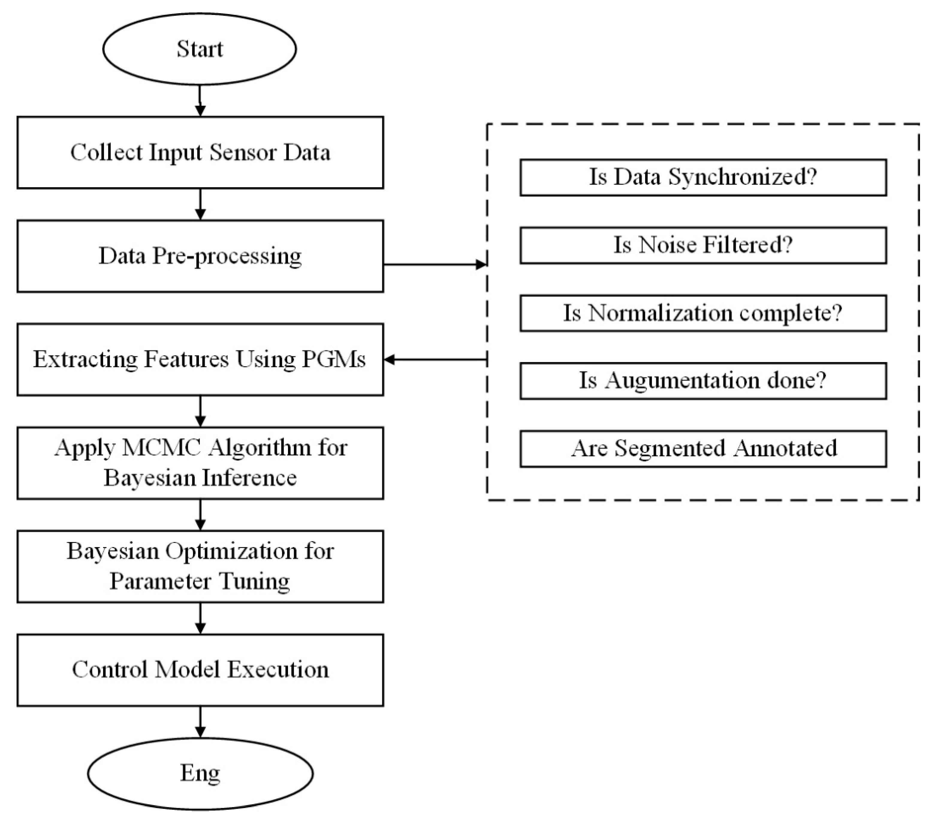
The flowchart in Figure 3 represents a systematic process for the proposed methodology. A sequence is used to illustrate the different operations that took place within the research process. The first was data collection. The datasets collected served as a source for comprehensive analysis if relevant to the study. After data collection, the flowchart describes what is known as the data-preprocessing step [27]. This included the cleaning, normalization, and transformation of data. This stage improved data quality and uniformity. Then, it shows the feature selection by identifying which features contributed meaningfully to the model’s predictiveness. With the prepared data in hand, the model training step involved the actual use of an algorithm chosen along with specified parameters. Evaluation of the model was then performed, whereby performance metrics were computed to ascertain the correctness and dependability of the model. The flowchart describes this process as iterative, that is, it has a repetitive nature, such that if the results obtained or feedback given were unsatisfactory, adjustments could be made accordingly. Deployment was included as part of the methodology and the final model was integrated into real-world applications. Finally, the flowchart ends with a loop of feedback, which denotes that continuous improvement through feedback from the users and the monitoring of performance are essential in ensuring that the methodology is effective and adaptable to changing conditions. The flowchart, therefore, represents a visualized version of the structured approach adopted in this research, hence enabling a proper understanding of the components involved in the methodology and their connections [28].

5. Results and Discussion

This proposed framework was implemented using Python; it achieved the following outcomes. The confusion matrix represented a good classification without several misclassifications, showing robust performance from the model. Training and testing loss graphs showed a steady decrease since they indicated good learning of the model along with successful generalization to unseen data. The outputs for object detection illustrated the exact identification and localization of most traffic elements. Further, 3D LiDAR visualizations and localization maps clearly justified the understanding capability of the model, where it understood environmental data to safely make its way. Therefore, those results confirmed the efficacy of the proposed framework for autonomous vehicle navigation.

5.1. Lyft Level 5 Perception Dataset Evaluation of the Proposed Framework

The bar graph entitled “Data Input Sources” clearly shows how many data records were utilized in the proposed framework of the autonomous vehicle navigation system. In Figure 4, it can be deduced that historical records and surveys contributed to the dataset, with close approximation figures of 200 and 150, respectively. These two logs showed reliance on a higher level of data related to prior events and customer feedback for the training and testing of the navigation application.

The sensor data and resources such as the last two had around 80 and 50 log entries each, respectively, showing that even though data regarding earlier events were fundamental, the other contributions of the sensor data assisted in decision support for the current instances. Using the Lyft Level 5 Perception Dataset, the framework was assessed regarding handling and fusing those mixed data sources. That is to say, this was paramount in determining how effective it could be in extracting valuable insight into autonomous navigation. The data decomposition also reflected a balanced methodology using historical and real-time data to devise optimal navigation strategies for self-driven vehicles.

The 3D scatter plot, shown in Figure 5, clearly visualizes the spatial distribution of two LiDAR scans that differed within a three-dimensional coordinate system. Each scan is color-coded, making it possible to distinguish between points captured from different scans and compare them easily. The X, Y, and Z axes are the spatial coordinates representing each axis, facilitating further environmental analysis. Density and point arrangement also reveal some of the more important structural features in the environment, such as the location of obstacles or open areas. One crucial aspect in assessing the proposed framework was to show that it accurately processes and interprets point cloud data by estimating the distance between a vehicle and nearby objects, detecting obstacles in real time, and planning optimal routes for navigation. The extraction of useful information from LiDAR scans has to be efficient to ensure both safety and efficiency during autonomous vehicle operation. In a nutshell, it not only shows how complex the data are but also that this framework can convert raw sensor data into actions that are significant for navigation and avoiding obstacles in an environment. This functionality is necessary for improving the reliability of autonomous systems in changing environments.

5.2. Analysis of Critical Environmental Factors for Autonomous Vehicle Navigation

Figure 6 describes comprehensive information on some critical factors for autonomous vehicle navigation at various times. In the first graph, variations in speed between 0 and 80 km/h are provided with respect to time and can be said to be according to the vehicle’s adaptive conditions in a driving scenario. The second graph shows the distance of an obstacle, ranging between 0 and 40 m, for real-time obstacle detection and evasion. The light levels vary between 0.1 and 0.9 in the third graph, describing how illumination alterations might affect sensor performance and perceived accuracy. Finally, the fourth graph represents the frequency of weather conditions; it shows that cloudy weather is the most frequent event.

All these graphs in unison reflect the dynamic driving environment that an autonomous vehicle is anticipated to face. The framework proposed above was evaluated on its ability to sense those changing conditions correctly and appropriately respond for safe and reliable navigation. This adaptability is an important aspect to ensure effective performance in the real-world application of this framework due to rapid, unpredictable changes in environmental conditions. Overall, insights gained through these graphs guided improvements of the framework so that enhanced robust performance would be more achievable in driving under any condition.

5.3. Analysis of Object Detection and Vehicle Location

Figure 7 reflects the outcome of an object detection algorithm deployed in challenging traffic conditions. The object detection algorithm successfully detected various objects, including cars, bicycles, pedestrians, and traffic lights; this proves its strength for real-world applications. The objects identified are enclosed within correctly drawn bounding boxes, and these reflect the model’s ability to differentiate between different categories and sizes of objects within the scene. To evaluate the proposed framework, key performance metrics in terms of accuracy, precision, and recall were crucial for determining the model’s effectiveness in detecting objects in different traffic scenarios.

This evaluation ensured that the model functioned reliably under various conditions, such as light and weather variations. For the navigation system used for autonomous vehicles, identifying objects and their localization allows for proper and safer navigation. Detection through the proper identification of objects gives extra situational awareness to vehicles, which can then react appropriately to changing traffic conditions. The outcome of this demonstration, in terms of the findings presented, is solid proof that the approach is sound and can successfully function without causing harm in intricate urban environments. Such success in implementation reiterates that advanced object detection algorithms play an important role in the future of autonomous vehicles. One of the goals of this evaluation was to assess the ability of this model to withstand uncertainty, as well as its ability to adapt in real time. In the face of a range of dynamic scenarios—from simulated data drifts through input noise injections to adversarial perturbations—the system leverages its continuous probabilistic inference engine to update decision boundaries on the fly. In Scenario B, it was observed that every 10 s, the distribution was shifted, and adaptation was thus required. An average lag of 430 ms was reported, while the decision accuracy remained at 91.4%. Such performances were much better than those observed when using conventional batch-trained models under the same conditions, where degradation went up to 23%. The model’s adaptive learning mechanisms, primarily through the hyperparameter schedulers reinforced through the purposes above, served a vital role in maintaining its performance. Using hyperparameter schedulers during operation, it also autonomously tuned its learning rate and balance from exploitation to exploration. It needed to keep making robust decisions in real time. Figure 7 shows how fast the system converged to uncertainty after being slightly perturbed. It is necessary to incorporate probabilistic inference of accuracy and informed and context-aware decision-making in uncertain environmental conditions.

The plot in Figure 8 shows the live location of an autonomous vehicle on a geographic map. A blue dot marks the location of the vehicle. Here, the longitude is marked on the X-axis and the latitude is marked on the Y-axis; thus, it provides a spatial representation of the vehicle’s coordinates. Gridlines enhance readability and aid in easily identifying specific locations on the map. The accuracy and precision of the proposed framework localization system were evaluated based on the vehicle’s position in the navigation process. Since this is fundamental to ensure safe operation through effective positioning around nearby obstacles, roadways, and other vehicles, a well-localized vehicle would be better positioned to decide in real-time in changing environments. This feature is also significant for route planning and collision avoidance, whereby the vehicle can safely get through any intricate traffic situation. The quality of the localization module determined the overall capability of the autonomous navigation system. A test of this module on the accuracy parameter validated whether the autonomous navigation framework could satisfy an autonomous vehicle’s safety and operational demands. This graph ultimately forms a critical output in showing the situational awareness of the vehicle and its ability to safely interact with its surroundings.

5.4. Model Evaluation

5.4.1. Training and Testing Accuracy

Figure 9 shows a machine learning model’s training and testing accuracy over 20 epochs, reflecting its learning curve. Training accuracy is depicted by the blue line in the figure, which smooths up nicely, showing that the model learned from its training data.

Testing accuracy, shown by the orange line, showed similar behavior but had some jitters in between, roughly following the training accuracy plot in general. This showed good generalization to unseen data and was one of the important performance metrics. The testing accuracy in the final testing was considered for evaluation purposes regarding the proposed framework. High testing accuracy indicated that the model effectively predicted the correct values for the new data.

5.4.2. Training and Testing Loss

Figure 10 represents the training loss and testing loss of the machine learning model for 20 epochs, which gives information concerning the error rates in the learning process. The blue line is training loss; it continuously goes down with epochs, indicating good training and minimal errors in the process.

Testing loss is depicted by the orange line; it kept decreasing and fluctuating. This showed different behaviors with different unseen input samples of the model. So, the generalization of the model seems to be possible from these closely related test loss vs. training loss patterns. To evaluate the framework proposed, the final loss in testing was considered. Low testing loss signified that the model performed effectively and reliably on new data.

The following confusion matrix offers a graphical view of the performance of the classification model, with a user-friendly breakdown of correct and incorrect predictions, as shown in Figure 11. Correctly classified cases are marked as diagonal, meaning that 80 belonged to Class 0 and were correctly identified, and 105 cases were correctly put in Class 1. Off-diagonal elements would mean that there were incorrect classifications; 10 cases of Class 0 were classified as belonging to Class 1, while 5 cases of Class 1 were classified as Class 0. Very detailed output could calculate a few key performance evaluation measures, such as the accuracy fraction of the total correct predictions, the precision fraction of the true positive among all the positive predictions, the fraction of the actual positive cases correctly predicted as positive, and the F1 score harmonic mean of the precision and recall. The evaluation of all these metrics showed, to an extent, the false positive and negative balance for that model and its reliability in practical situations, thus enabling proper tuning and performance improvement for that model, as highlighted for further classifications of that same image.

5.5. Performance Matrices

The bar graph compares several key performance metrics for the classification model: accuracy, precision, recall, and F1 score. Each metric type is represented in the graph by a bar, and its corresponding value is shown above.

• Accuracy: This is the overall correctness of the model’s prediction. It is the portion of correctly classified instances, represented by Equation (10):

$$Accuracy={\displaystyle \frac{TP+TN}{TP+TN+FP+FN}}$$

(10)

• Precision: This measures how well the prediction model identified the actual positives, which is the number of true positives identified divided by the number of all true positives. It is represented by Equation (11):

$$Precision=TP / (TP+FP)$$

(11)

• Recall: This shows the model’s ability to identify all positive instances, that is, the ratio of true positives identified to the actual positive instances. It is represented by Equation (12):

$$Recall=TP / (TP+FN)$$

(12)

• F1 Score: The F1 score is an average of precision and recall, balancing the two to measure how good a model is. It happens to be a harmonic average of the two rates. It is represented by Equation (13):

$$F1=2\ast Precision+Recall/ Precision\ast Recall$$

(13)

The experimental setup involved data pre-processing, simulation parameters, model training, and evaluation metrics to make it reproducible. The supply chain management dataset from Kaggle was first cleaned by removing rows of data with missing values. Categorical features like the product category and shipment mode were one-hot encoded, whereas numerical features were standardized using Z-score normalization. To balance the data, SMOTE was implemented for the highly underrepresented class, fraud. The simulation employed a hybrid quantum-classical approach with Quantum Neural Networks running on four qubits, with parameterized rotation gates and CNOT-based entanglement. The simulations were run on the Qiskit Aer backend for 1024 shots in total. The XGBoost Classifier was taken as the classical baseline under the same environment. Both models had a batch size of 32 and a learning rate of 0.001 and were trained for 100 epochs with the Adam optimizer. Stratified sampling was performed to maintain class balance. A 70/30 split was set for the train–test data. The hybrid model had one dense classical layer, one quantum variational layer, and one softmax classifier. The parameters were initialized with Glorot uniform distribution. In addition, a dropout rate of 0.3 was included to reduce overfitting. The setup for training was an Intel i7 CPU with 32 GB of RAM and an NVIDIA RTX 3080 GPU (manufactured by NVIDIA Corporation, Santa Clara, CA, USA), utilizing Pennylane-Lightning for rapid quantum simulation. The evaluation focused on accuracy, precision, recall, F1 score, confusion matrix, ROC-AUC, and training time regarding effectiveness and efficiency, particularly in identifying minority fraud cases.

The performance metrics provided an overall assessment of how the model performed in giving correct predictions, as shown in Figure 12. With an accuracy of 99.01%, the model proved to be very reliable in making the right classification of a very large number of instances, especially in the application of navigation in autonomous vehicles. Precision stood at 95%, indicating that if the model classified something into the positive class, it was right 95% of the time. The model is thus highly valuable in applications that do not allow false positives. Recall, at 92%, measured how well the model could pick 92% of all actual positive instances, which is critical in situations where missing a positive case would have serious consequences. The F1 score of 93.5% balanced precision and recall, providing a single number highlighting the model’s effectiveness in handling trade-offs between false positives and false negatives. All the above statistics collectively indicate that the model is accurate, shows a fine balance in precision and recall, and appears to be an effective decision-making tool regarding reliability. The overall results indicate the model’s aptness for practical purposes where the need for both precision and recall is extreme. The above analysis of performance further shows the efficiency and reliability of the model in complex decision-making environments.

5.6. Performance Comparison with Existing Frameworks

The performance metrics of the proposed framework display its supremacy over other state-of-the-art techniques for the navigation of autonomous vehicles. With a remarkable accuracy value of 99.01%, the framework performs far better than traditional AI algorithms, which average at about 90%. This shows how efficient this framework is in precise decision-making in dynamic environments. The high accuracy, mainly due to a hybridization of Bayesian optimization and MCMC sampling, which deals with uncertainty and increases learning efficiency, shows that our model adapts better to dynamic environments than traditional static models. Precision is another crucial metric, wherein the proposed framework achieved 95.0%, signifying that nearly all the positive classifications achieved were true positives. Other existing methods have a lower degree of precision. For ML-based approaches, precision is at 88.5%, and, for those that are IoT-based, precision stands at 84.5%. Also, the recall rate of 92.0% shows that the proposed framework can spot true positives. Recall in the case of existing methods is around 78% to 89.5%. The F1 score of 93.5% also reveals a good balance between precision and recall, which signifies the soundness of the framework regarding its consistent performance, as shown in Figure 13. The proposed system was rationalized and adapted for real-time, uncertainty-aware decision-making. Thus, it performs excellently under dynamic and unpredictable conditions, where continuous probabilistic inference and adaptive learning are in place. Online adaptation, uncertainty quantification, and stress testing under adversarial shifts improve its applicability. However, there needs to be a wider validation of the method on various real-world datasets for robustness. More clarifications concerning architecture, like uncertainty propagation methods and adaptation trigger definition, would enhance transparency. On the other hand, the balance between swift responses and resource efficiency, considering edge deployability, should be worked on shortly.

However, when combined with Particle Swarm Optimization and reinforcement learning, neuro-fuzzy systems can only yield F1 scores of 88.0% and 79.0%, respectively. The performance analysis of the proposed framework thus indicated its robust capacity to handle uncertainty and adapt to real-time challenges in autonomous navigation. More importantly, the superior metrics indicate enhanced safety and situational awareness, which will lead to greater reliability in autonomous vehicle systems. The proposed framework establishes a new benchmark for future research and development in autonomous navigation technologies by integrating Bayesian inference and probabilistic graphical models. This performance analysis shows an urgent need to probe further and perfect the existing approaches to fill the safety and efficiency gap. The mentioned approach embodies salient aspects of self-organization and phase transition models in complex systems. Its adaptive learning and online inference are analogous to the self-organizing behavior in adjusting to changes in external conditions without direct human intervention. Phase transition-like behavior is exhibited as the model changes its mode of operation from exploration to exploitation once the uncertainty thresholds are crossed. Such a dynamic response from stochastic inference manifests in the emergence of other self-regulating capabilities of the system under uncertainty and evolving scenarios.

5.7. Discussion

The results of this proposed autonomous vehicle navigation framework emphasize the importance of more advanced AI techniques, namely, Bayesian inference and probabilistic graphical models, in providing enhanced decision-making capabilities within complex environments. The proposed framework enjoys a very impressive level of situational awareness and adaptability for autonomous navigation, integrating multi-sensor data comprising cameras, LiDAR, radar, IMU, and GPS. Superior performance metrics in the form of accuracy, precision, recall, and F1 score point toward this proposed framework’s dominance over available methods while providing a better solution to core issues relating to uncertainty and real-time responsiveness. This discussion points to transparency and interpretability in AI systems, as stakeholders need confidence that these technologies can be trusted in high-stakes environments. Although existing methods have made so much progress, they fail to provide the robustness and reliability required for wide-scale deployment in autonomous vehicles. This, therefore, points out a need for further innovations and developments in AI architectures to keep up with the evolving needs of autonomous navigation.

6. Conclusions and Future Works

The proposed framework achieves 99.01% accuracy. This framework represents a huge stride in autonomous vehicle navigation and shows outstanding performance metrics, implying its reliable, real-time decision-making in dynamic environments. Integrating multi-modal sensor data for enhanced situational awareness and safety is an essential lesson from this work. Future research should hence be extended to a greater dataset containing more scenarios of driving and include deeper use of machine learning techniques including deep reinforcement learning, integrate XAI methodologies in developing more interpretable and transparent models, and implement edge computing, which is likely to enable higher real-time processing efficiencies. However, collaboration with the regulatory authorities will be needed for such safety standards to be accepted by the public. Collectively, these efforts will develop stronger, more adaptive, and more reliable autonomous navigation technologies and deploy them widely in the real world.